FFUOV-99/03

hep-th/9903039

ON THE MICROCANONICAL DESCRIPTION

OF D-BRANE THERMODYNAMICS

Marco Laucelli Meana and Jesús Puente Peñalba

Dpto. de Física, Universidad de Oviedo

Avda. Calvo Sotelo 18

E-33007 Oviedo, Asturias, Spain

Abstract

We study the microcanonical description of string gases in the presence of D-branes. We obtain exact expressions for the single string density of states and draw the regions in phase space where asymptotic approximations are valid. We are able to describe the whole range of energies including the SYM phase of the D-branes and we remark the importance of the infrared cut-off used in the high energy approximations. With the complete expression we can obtain the density of states of the multiple string gas and study its thermal properties, showing that the Hagedorn temperature is maximum for every system and there is never a phase transition whenever there is thermal contact among the strings attached to different D-branes.

1 Introduction

Finite temperature frameworks are in general very interesting laboratories in which to study the fundamental degrees of freedom of a theory. In the case of string theory the interest increases because of the exponential growth of the number of states with the mass. This behavior, known as the Hagedorn spectrum [1], is relevant because of the fact that it generates a critical thermodynamics that in principle could correspond to a phase transition [2, 3, 4, 5]. The analysis of this possibility was firstly attempted from the canonical ensemble [2, 3, 4, 5], but it seems that a more fundamental description of the degrees of the system is needed.

The description that, in principle, would clarify the open questions on the Hagedorn thermodynamics is that of the microcanonical ensemble [7, 6, 8, 9]. The density of states of the string gas was studied in the early works [7, 6] on the subject by taking an ambiguous high energy approximation. In fact the thermodynamics for the closed strings that was derived there do not have any information about the low energy behavior of the system. This prevents any trustable study on the way the system reaches the Hagedorn temperature.

On the other hand in [7, 6] there was a disregarding of the volume dependence on the density of states that led to the surprising conclusion that there is a difference between a system with an already open universe and one in which we take to infinity the radii of the initial torus [6].

In [8, 9] another point of view was claimed. The density of states of the single closed string valid for all energies was obtained. The multiple string one was formally defined from the convolution theorem [8], and it was shown that for an already open universe the systems reaches the Hagedorn temperature for a finite energy per string. At this point a phase transition occurs in such a way that the temperature is kept constant and the specific heat diverges. By this analysis it was possible to know how the systems evolve from low energy to the high energy limit.

The compactified case was studied in [9]. In this background the system has a unique phase with finite and positive specific case. The Hagedorn temperature works as the limiting one. An interesting point was that in the decompactification limit the system coincided with that of [8].

A common feature appearing in both cases is that at high energies equipartition breaks at a given energy per string. From this point the system is composed of a dominant highly energetic long string in thermal contact with a sea of a large number of low energetic strings that works as a thermal bath. This relevant part of the system was not taken into account previously in [7, 6] because it emerges from the IR part of the single string density of states. The existence of the string sea is relevant in order to prevent the negative specific heat phases.

From an completely different perspective the same picture has been recently obtained [16]. The authors of [16], considered the possibility of a high energetic radiating string. They discovered that this string would behave as a black body at a temperature $T_{H}$ and if one included a thermal bath composed by low energetic strings the system would reach equilibrium only if both temperatures, those of the black body and those of the bath, coincide at the Hagedorn value. This strongly supports the idea presented in [8, 9], that a long energetic string would be in thermal equilibrium only in the presence of a thermal bath at $T_{H}$.

To put it in short: working with approximate expressions without a neatly defined range of validity is dangerous. It is difficult to discern in which situations low energy effects can qualitatively change the conclusion of the physical analysis. This is specially true in systems composed of many objects, let alone those where a thermodynamical limit is to be taken and even more near a phase transition, because local and small fluctuations compared to the total energy can always make individual objects visit the regions of phase space that have been thrown away. In our work we will render an exact calculation of the single string density of states and a comparison with the different approximation that come from it will be done.

These considerations hold for perturbative string physics. It has been sometimes argued that non-perturbative objects would have some role to play in relation to the Hagedorn problem. There have been some works in which this topic has been dealt with, either trying to include D-branes [15] in the canonical ensemble [10, 11, 12], or D-instantons [13] effects in the microcanonical ensemble. A laconic ’nothing happens’ has been the usual conclusion. In the former case the problem of approaching the Hagedorn problem from the canonical ensemble is exactly the same that for closed strings. That is the canonical description breaks and nothing else could be said since this point. In the latter the main argument is that the energy scales at which the non-perturbative effects become important are completely dominated by the perturbative Hagedorn physics, so it seems natural to conclude that a subsequent effect cannot regularize an already existing at low energies one.

D-brane dynamics is governed by the Dirichlet open strings attached to it [15], so in order to study D-brane thermodynamics we need to study the finite temperature version of these open string theories [10, 11, 12]. On the other hand if we want to study the complete thermal behavior of type II string theories we need to account for the closed string sector and for the corresponding D-branes allowed for each theory. Finally if we want a fundamental understanding of the Hagedorn ’phase’ of the theory we need to study it in the microcanonical ensemble. This idea has been recently developed in [18].

In this work the microcanonical density of states has been computed for a variety of brane configurations by using the methods of [6, 7], and high energy thermodynamics has been described. A related work was also made in [14].

In the present paper we approach the microcanonical description of thermodynamics with D-branes as background applying the methods of [8, 9]. The plan of the work is the following. We begin the analysis by computing the density of states from the mass spectrum. The next step consists of a computation of the single string density of states by the method of the inverse Laplace transform. We separate the analysis for high energies, analogous to the analysis of [18], from those valid for the whole energy range. Using the previous results we go to the thermodynamical description of the system .

2 The Density of States from the Mass Spectrum

There are two ways to compute the density of states of the single string system. The first one consists of the application of the inverse Laplace transform. The method begins with the computation of the Helmholtz free energy and then using it as the single string partition function in such way that we obtain the density of state from the Bromwich integral

$$\Omega^{(1)}(E)=\frac{1}{2\pi i}\int_{C}d\beta Z_{1}(\beta)e^{\beta E}$$ (1)

where $Z_{1}(\beta)=-V\beta F(\beta)$. The $n$-string term is characterized by the partition function

$$Z_{n}(\beta)=\frac{1}{n!}Z_{1}(\beta)^{n}.$$ (2)

The other way to calculate the microcanonical density of states of a system is to count the degeneracy in the phase space geometrically. It is specially useful in the case of compact target backgrounds. In this section we shall implement this idea in our case of a gas of open superstrings moving in the presence of D-branes. We start with the following Hamiltonian, that corresponds to the mass formula of the theory which. We take it as a dispersion relation

$$\alpha^{\prime}E^{2}=\vec{p}^{2}+\vec{\omega}^{2}+2N$$ (3)

where $\vec{p}$ is the momentum, that is discrete in this case. The dimension of this vector is the number of Neumann directions. $\vec{\omega}$ is the winding number. It is always perpendicular to the momentum vector because open strings cannot wind around a direction and have a momentum at the same time. The dimension of this vector is, thus, the number of Dirichlet directions. $N$ is the total oscillation number. It is the sum

$$N=\sum nN_{n}.$$ (4)

This means that there are several states with the same total oscillator number. They are counted by the following coefficients:

$$a_{k}=\frac{1}{2\pi i}\oint\frac{dq}{q^{k+1}}\left(\frac{\vartheta_{2}(q)}{\eta^{3}(q)}\right)^{4-\frac{\nu}{2}}\left(\frac{\vartheta_{3}(q)}{\vartheta_{4}(q)}\right)^{\frac{\nu}{2}}$$ (5)

where the integrand is the internal partition function of the theory .

Let us begin to calculate the degeneracy associated to a value of the energy fixing firstly $N$ to a constant. In that case:

$$\vec{p}^{2}+\vec{\omega}^{2}=\alpha^{\prime}E^{2}-2N=C$$ (6)

On the other hand

$$\vec{p}^{2}+\vec{\omega}^{2}=\sum_{i\in NN}n_{i}^{2}\frac{\alpha^{\prime}}{R_{i}^{2}}+\sum_{i\in DD}\frac{R_{i}^{2}}{\alpha^{\prime}}$$ (7)

where $NN$ marks the directions with Neumann boundary conditions and $DD$ the Dirichlet ones, there are also mixed directions, $DN+ND=\nu$, that do not contribute to the kinematical energy but through their oscillator masses only. This contribution is accounted by the coefficients $a_{N}$ . To make things more homogeneous, we can use the variables

$$r_{i}=\frac{R_{i}}{\sqrt{\alpha^{\prime}}}\hskip 56.9055pt\mbox{if $i$ is Neumann}$$

$$r_{i}=\frac{\sqrt{\alpha^{\prime}}}{R_{i}}\hskip 56.9055pt\mbox{if $i$ is Dirichlet}$$ (8)

so that

$$\vec{p}^{2}+\vec{\omega}^{2}=\sum_{i}\frac{n_{i}^{2}}{r_{i}^{2}}=C$$ (9)

this is the equation of an ellipsoid in the discrete phase space. We are interested in counting the number of states for which that relation approximately holds, that is, letting the energy be in $[E-\Delta E,E+\Delta E]$. If the energies are very low, it is important to remind that $\Delta E$ has a lower bound which is the maximum gap between two energy levels. The number of states is proportional to the volume of the ellipsoidal shell defined by equation (9). The total volume is

$$V(C)=\Omega_{\tilde{D}}\left(\prod_{i}r_{i}\right)C^{\tilde{D}/2}.$$ (10)

The volume of a thin shell is

$$V_{\mbox{\tiny shell}}=\Omega_{\tilde{D}}\frac{\tilde{D}}{2}\left(\prod_{i}r_{i}\right)C^{\frac{\tilde{D}}{2}-1}\Delta C=$$

$$=\Omega_{\tilde{D}}\tilde{D}\left(\prod_{i}r_{i}\right)\left(\alpha^{\prime}E^{2}-2k\right)^{\frac{\tilde{D}}{2}-1}\alpha^{\prime}E\Delta E$$ (11)

where $\Omega_{\tilde{D}}$ is the angular part. Its dependence on the dimension is

$$\Omega_{\tilde{D}}=\frac{2\pi^{\tilde{D}/2}}{\tilde{D}\Gamma(\tilde{D}/2)}$$ (12)

In our case $\tilde{D}=DD+NN\leq 9-\nu$, is the number of testable directions.

To get the total degeneracy it is necessary to multiply by the one associated to $N$ ($a_{N}$) and by the size of the super-multiplet: $2^{4}$. After the sum over all possible values of $N$ is performed, the result is

$$\Omega_{\mbox{\tiny cl}}(V,E)=2^{4}\frac{2\pi^{\tilde{D}/2}}{\Gamma(\tilde{D}/2)}(2\pi)^{DF-NN}\frac{V_{NN}}{V_{DD}}\sum_{N=0}^{\infty}a_{N}\alpha^{\prime}E\left(\alpha^{\prime}E^{2}-2N\right)^{\frac{\tilde{D}}{2}-1}{\cal H}\left(\alpha^{\prime}E^{2}-2N\right)$$ (13)

This is not valid for $\tilde{D}=0$ because the derivative in (11) is not correct. In that case there is no continuous contribution from either the momenta or the windings and do the density of states is just a sum of delta functions centered on the mass levels. We shall talk further in section $5$.

For a value of $E$, the sum over $N$ is finite because the oscillator number is limited by the available energy. This is expressed by the Heaviside function. The calculation will be complete when we take into account the quantum statistics. Before doing that, let us add some terms that are important if the proportion between some radii is very different from one. In that case, there is a range of energies where the first non-zero modes of some directions lie far beyond the ellipsoid in the phase space and the geometric count is no longer valid because the single zero mode is not counted as one but as a small fractional number of states. To simplify, we shall consider all the Neumann radii equal and the same with the Dirichlet ones. The only parameters are then $R_{DD}$ and $R_{NN}$. This can be generalized to consider all the possibilities but there are too many and all the interesting physical consequences can be extracted studying this simpler case. The density of states that this yields is

$$\Omega_{\mbox{cl}}(V,E)=2^{4}\frac{2\pi^{\tilde{D}/2}}{\Gamma(\tilde{D}/2)}(2\pi)^{DD-NN}\frac{V_{NN}}{V_{DD}}\sum_{N=0}^{\infty}a_{N}\alpha^{\prime}E\times$$

$$\times\left(\alpha^{\prime}E^{2}-2N\right)^{\frac{\tilde{D}}{2}-1}{\cal H}\left(\alpha^{\prime}E^{2}-2N\right){\cal H}\left(E-V_{C}^{-1/C}\right)+$$

$$+2^{4}\frac{2\pi^{C/2}}{\Gamma(C/2)}\frac{(2\pi)^{C}}{V_{C}}\sum_{N=0}^{\infty}a_{N}\alpha^{\prime}E\left(\alpha^{\prime}E^{2}-2N\right)^{\frac{C}{2}-1}{\cal H}\left(\alpha^{\prime}E^{2}-2N\right){\cal H}\left(V_{C}^{-1/C}-E\right)$$ (14)

where

$$\mbox{If}\hskip 28.45274ptR_{NN}\gg 1/R_{DD}\hskip 28.45274pt C \hskip 28.45274pt\mbox{stands for $NN$ and}\hskip 28.45274ptV_{C}=V_{NN}$$

$$\mbox{If}\hskip 28.45274ptR_{NN}<<1/R_{DD}\hskip 28.45274pt C \hskip 28.45274pt\mbox{stands for $DD$ and}\hskip 28.45274ptV_{C}=1/V_{DD}$$ (15)

Now it is easy to add quantum statistics following this recipe

$$-\beta F(\beta,V)_{B,F}=\pm\sum_{\{n\}}log\left(1\mp e^{\beta E(\{n\})}\right)=$$

$$=\mp\sum_{\{n\}}\sum_{r=1}^{\infty}\frac{(\pm 1)^{r}}{r}e^{\beta E(\{n\})}$$ (16)

This leads to the final result

$$\Omega(V,E)=2^{4}\frac{2\pi^{\tilde{D}/2}}{\Gamma(\tilde{D}/2)}(2\pi)^{DD-NN}\frac{V_{NN}}{V_{DD}}\sum_{N=0}^{\infty}\sum_{r\geq 1,\mbox{odd}}^{\infty}\frac{1}{r^{\tilde{D}+1}}a_{N}\alpha^{\prime}E\times$$

$$\times\left(\alpha^{\prime}E^{2}-2Nr^{2}\right)^{\frac{\tilde{D}}{2}-1}{\cal H}\left(\alpha^{\prime}E^{2}-2Nr^{2}\right)+$$

$$+2^{4}\frac{2\pi^{C/2}}{\Gamma(C/2)}\frac{(2\pi)^{C}}{V_{C}}\sum_{N=0}^{\infty}a_{N}\alpha^{\prime}E\left(\alpha^{\prime}E^{2}-2N\right)^{\frac{C}{2}-1}{\cal H}\left(\alpha^{\prime}E^{2}-2N\right){\cal H}\left(V_{C}^{-1/C}-E\right).$$ (17)

This result is completely analogous to that of [9]. We will see in next sections how we can recover the same density of states for the single string system from the study of the free energy of the theory in the canonical ensemble.

3 High Energy Density of States

In this section we are going to compute the Helmholtz free energy of the Dirichlet open string theory for a variety of D-brane backgrounds from the canonical ensemble, and we will finally study the different limits of the density of states derived from it. We will do it for the asymptotic high energy range. The approximation is based on the idea that the existence of the Hagedorn critical temperature is an UV phenomenon so it should be enough to look at the very excited string states to obtain the relevant information, this is the perspective assumed in [6, 7], and more recently, for the D-brane backgrounds, in [18]. The other option is to try to compute the complete density of states without projecting out any string states, and will be detailed in the section 5.

We will begin by noticing that the degrees of freedom lost in this high-energy limit, are, in fact, projected out in the canonical description by a IR cut-off that cannot be forgotten. If we introduce it explicitly, we would easily see how the massless open strings are neglected. This projection prevents the possibility of accounting for the low energetic sea.

Let us firstly fix our background. Suppose we have a configuration with a Dp-brane and a Dq-brane. We can define four different types of directions, the Dirichlet-Dirichlet(DD),Neumann-Neumann (NN), ND and DN. The last two do not contribute to the mass of the strings, apart from the oscillation terms (That means that we can neither have momentum nor winding in these directions). We will include in this classification of the directions the spatial ones only. They are related by

$$DD+NN+DN+ND=9.$$ (18)

The Euclidean time is supposed to be compactified on a circle of length $\beta$. Another interesting parameter we will deal with is the sum of the mixed directions, $\nu=ND+DN$. The interest of it comes from the fact that the when $\nu=0,4,8$ the string gas is evolving in a completely supersymmetric background. We will focus our study on this type of brane configuration, however some comments on more general ones will be made.

In brief, the string’s quantum numbers are: the momentum mode in the NN directions; the winding mode in the DD ones and the Matsubara frequency in the Euclidean time, the DN and ND direction do not contribute to the mass of the strings.

We can now compute the Helmholtz free energy as the vacuum energy of the theory described above. It formally reads

$$-\beta F(\beta)=-Tr_{H}(-1)^{F}\int_{0}^{\infty}\frac{dt}{2t}e^{-2\pi\alpha^{\prime}tM^{2}}$$ (19)

where $M$ is the mass of the string and is given by

$$M^{2}=\sum_{i=1}^{NN}\frac{n^{2}_{i}}{R_{i}^{2}}+\sum_{i=1}^{DD}w^{2}_{i}R_{i}^{2}+\frac{4\pi^{2}m^{2}}{\beta^{2}}+Osc$$ (20)

where the last contribution comes from the oscillator modes of the open string. We can compute the trace over the Hilbert space obtaining

$$-\beta F(\beta)=-\int_{0}^{\infty}\frac{dt}{2t}\prod_{i}^{NN}\theta_{3}\left(0,\frac{2it\alpha^{\prime}}{R_{i}^{2}}\right)\prod_{i}^{DD}\theta_{3}\left(0,2it\alpha^{\prime}R_{i}^{2}\right)\theta_{4}\left(\frac{8\pi^{2}it\alpha^{\prime}}{\beta^{2}}\right)f(t)$$ (21)

where the internal partition function $f(t)$ is given by

$$f(t)=\left(\frac{\vartheta_{2}(0,it)}{\eta^{3}(it)}\right)^{4-\frac{\nu}{2}}\left(\frac{\vartheta_{3}(0,it)}{\vartheta_{4}(0,it)}\right)^{\frac{\nu}{2}}.$$ (22)

The high energy behavior of the open string gas may be studied in the canonical ensemble and that is the easiest way of visualizing the Hagedorn critical behavior. Let us begin our study by looking at this region. When the energy is large the string modes that dominate the dynamics will be the massive ones. These are enclosed in the UV region of the previous expression, that is accounted by the large $t$ limit. We can introduce an IR cut-off $\Lambda^{2}$ in (21), and in this way we will forget about low energetic strings, we have

$$-\beta F(\beta)=-\int_{0}^{\Lambda^{2}}\frac{dt}{2t}\prod_{i}^{NN}\theta_{3}\left(0,\frac{2it\alpha^{\prime}}{R_{i}^{2}}\right)\prod_{i}^{DD}\theta_{3}\left(0,2it\alpha^{\prime}R_{i}^{2}\right)\theta_{4}\left(\frac{8\pi^{2}it\alpha^{\prime}}{\beta^{2}}\right)f(t)$$ (23)

In order to study the UV limit ($t\rightarrow 0$) it is convenient to take advantage of modular properties of the theta functions in the free energy going to the closed-string channel by making $t=2\pi^{2}s^{-1}$, obtaining

$$-\beta F(\beta)\sim-\frac{V^{NN}}{V^{DD}}\frac{\beta}{4\pi}\int_{\frac{2\pi^{2}}{\Lambda^{2}}}^{\infty}ds\prod_{j}^{NN}\theta_{3}\left(0,\frac{iR_{j}^{2}s}{4\pi^{2}\alpha^{\prime}}\right)\prod_{j}^{DD}\theta_{3}\left(0,\frac{is}{4\pi^{2}R_{j}^{2}\alpha^{\prime}}\right)$$

$$\times\theta_{4}\left(0,\frac{i\beta^{2}s}{16\pi^{3}\alpha^{\prime}}\right)\left(\frac{\vartheta_{4}(0,\frac{is}{2\pi^{2}})}{\eta^{3}(\frac{is}{2\pi^{2}})}\right)^{4-\frac{\nu}{2}}\left(\frac{\vartheta_{3}(0,\frac{is}{2\pi^{2}})}{\vartheta_{2}(0,\frac{is}{2\pi^{2}})}\right)^{\frac{\nu}{2}}$$ (24)

We can now go to the large $s$ limit by simply taking into account that

$$\lim_{s\rightarrow\infty}\left(\frac{\vartheta_{4}(0,\frac{is}{2\pi^{2}})}{\eta^{3}(\frac{is}{2\pi^{2}})}\right)^{4-\frac{\nu}{2}}\left(\frac{\vartheta_{3}(0,\frac{is}{2\pi^{2}})}{\vartheta_{2}(0,\frac{is}{2\pi^{2}})}\right)^{\frac{\nu}{2}}=e^{s/2\pi},$$ (25)

we finally can express the UV limit of the open string free energy, with the correct multiplicative prefactors, as

$$-\beta F(\beta)=-\frac{V^{NN}}{V^{DD}}(2\pi)^{DD-NN}(2\alpha^{\prime})^{\frac{\nu-10}{2}}\frac{\beta}{4\pi}(2\pi^{2})^{-1}\sum_{\{M,n\}}\int_{\frac{2\pi^{2}}{\Lambda^{2}}}^{\infty}ds\,e^{-s\Delta(M,n,\beta)}$$ (26)

where we have defined

$$\Delta(M,n,\beta)=M^{2}+\frac{n^{2}\beta^{2}}{16\pi^{2}\alpha^{\prime}}-\frac{1}{2\pi},$$ (27)

in that way the winding and momentum modes are included into the mass $M$. In what follows we will collect the numerical factors into a multiplicative constant $C$. When $\Delta(M,n,\beta)=0$ we arrive at a critical temperature analogous to the Hagedorn one. In fact we can see that at those temperatures a string state becomes massless. When the temperatures are passed through this states get a negative squared mass, that is, it becomes tachyonic. We can solve the equation for the critical temperatures obtaining

$$\beta_{c}^{2}=\frac{8\pi\alpha^{\prime}}{n^{2}}-\frac{16\pi^{2}\alpha^{\prime}M^{2}}{n^{2}}\,\,\,\,\,\hbox{with}\,\,\,\,0<n\in{{Z}}.$$ (28)

With $n=1$ and $M=0$ we have the lowest critical temperature that corresponds to the Hagedorn one. The following critical points are obtained for bigger temperatures, in fact we can in principle have negative unphysical solutions for $\beta_{c}$. This possibility is avoided by assuming that the compactification radii are bigger than the selfdual ones.

At this moment we can write the Helmholtz free energy as a sum over functions which are analytical in the whole complex-$\beta$ plane except in the neighborhood of $\beta_{c}$. The sum reads

$$-\beta F(\beta)=-C\frac{V^{NN}}{V^{DD}}\frac{\beta}{4\pi}\sum_{\{\beta_{c},n\}}\int_{\frac{2\pi^{2}}{\Lambda^{2}}}^{\infty}ds\,e^{-\frac{sn^{2}}{2\pi}\left(\frac{\beta^{2}-\beta_{c}^{2}}{\beta_{H}^{2}}\right)}.$$ (29)

Finally we can integrate the previous expression in order to obtain a closed expression for the free energy in the high energy limit. Using the integral representation of the incomplete Gamma function we have

$$-\beta F(\beta)=-C\frac{V^{NN}}{V^{DD}}\frac{\beta}{4\pi}\sum_{\{\beta_{c},n\}}\left[\frac{n^{2}}{2\pi}\left(\frac{\beta^{2}-\beta_{c}^{2}}{\beta^{2}_{H}}\right)\right]^{-1}\Gamma\left(1,\frac{\pi n^{2}}{\Lambda^{2}}\left(\frac{\beta^{2}-\beta_{c}^{2}}{\beta^{2}_{H}}\right)\right).$$ (30)

The problem of obtaining the single string density of states from the free energy below is reduced to an inverse Laplace transformation. It is known that the result of this kind of computation is closely related with the analytical properties of the function to be transformed. We can look at (30) as a sum of independent terms seeing that each one is characterized by its behavior in the neighborhood of its thermal critical point $\beta_{c}$. We see that the analytical properties are enclosed in the simple pole and in the more complicate properties of the incomplete Gamma function. The computation of the density of states here would consist of a straightforward adaptation of those in [8].

Before showing the results of the computation let us comment some words about the cut-off $\Lambda^{2}$. We can try to extend the validity of the approximation taking the value of $\Lambda^{2}$ to infinity. It will give us the complete version of the Gamma function. The analytical properties of the Free Energy are enclosed inside the single pole appearing at each critical temperature. If we complete the IR part of the Free Energy by simply taking $\Lambda^{2}$ to infinity we will obtain an IR regular series for the density of states of the single string. The thermodynamics derived from it would have a positive and finite specific heat phase only, in which the asymptotic maximum temperature is the Hagedorn one. We think that this corresponds to a misconception. The IR behavior that one could obtain from the previous procedure is at least not complete. It is due to the fact that if we took a large $\Lambda^{2}$ limit we could not truncate the string theory partition function as we did in (25), but we should have included all the string modes.

We think that the correct way of using the previous free energies consist of keeping $\Lambda^{2}$ finite, and making inverse Laplace transformation of the Laurent series around the critical points. Doing it we will see that we obtain an asymptotic series that does not work for the IR regime.

Following the previous prescriptions we can make the same computation of the high energy single string density of states as in [8], it gives

$$\Omega^{(1)}(E)=\frac{V^{NN}}{V^{DD}}\sum_{\{\beta_{c},n\}}\sum_{p=0}^{1}\sum_{m=0}^{\infty}A(\beta_{c},n,m,p)\frac{(-1)^{m+p}e^{\beta_{c}E}}{E^{m+p}}{\cal H}\left(E-\frac{2\pi\beta_{c}n^{2}}{\beta_{H}^{2}\Lambda^{2}}\right)$$ (31)

where $A(\beta_{c},n,m,p)$ is a constant independent of $E$ but dependent, through $\beta_{c}$, of the $R$ parameters, and ${\cal H}(x)$ is the Heaviside function. The sum in $m$ comes from a Taylor expansion of the incomplete Gamma function.

The behavior is in general governed by a leading term that corresponds to the Hagedorn singularity. We will come back to the details later but let us sketch the general dynamics. We find a positive, but infinite, specific heat phase. The leading term does not give any negative powers of the energy taking us to theory with a constant temperature and infinite specific heat behavior. The subleading terms give corrections for small energies. The string gas takes a finite and positive specific heat phase.

We think that these corrections are meaningless because the density of states is only valid for a very high energy, and in order to know the low energetic phase we need an IR-complete density of states. We will come back on these features later when studying the thermodynamical behavior of the gas.

It seems interesting to study the high energy density of states when we open some of the DD directions. This case physically means that there would be a reduced number of testable directions for the single string and has shown its interest in previous studies [7, 18, 17]. The result is analogous to (31). It is implemented by taking some of the $DD$, (let it be a number $0\leq a\leq DD$ of them), infinite. We will also suppose that the momenta on the $NN$ directions are continuous so

$$R^{DD}_{1},...,R^{DD}_{a},R^{NN}_{1},...,R^{NN}_{NN}\rightarrow\infty.$$ (32)

Including it into (24), and then also in(28), we arrive at the following UV canonical Free Energy

$$-\beta F(\beta)=-C\frac{V^{NN}}{V^{DD-a}}\frac{\beta}{4\pi}\sum_{\{\beta_{c},n\}}\left[\frac{n^{2}}{2\pi}\frac{(\beta^{2}-\beta_{c}^{2})}{\beta^{2}_{H}}\right]^{\frac{(9-\tilde{D}-\nu)}{2}-1}\Gamma\left(1+\frac{\tilde{D}+\nu-9}{2},\frac{\pi n^{2}}{\Lambda^{2}}\frac{(\beta^{2}-\beta_{c}^{2})}{\beta^{2}_{H}}\right).$$ (33)

where $\tilde{D}$ is defined as a effective number of testable dimensions. It is given by

$$\tilde{D}=(DD-a)+NN\leq 9-\nu.$$ (34)

The meaning of this number of dimensions and the existence of ’testable’ energy scales will be discussed later.

In this case the ananlytical properties are more complicate. In general we can see that we have a branch point located at each critical temperature, concretely it will happens for an odd number of untestable $DD$ directions, while for even ones we would have high order pole singularities. The IR continuation, by taking $\Lambda^{2}$ to infinity, is not well defined here. The density of states that results from inverse Laplace transform (33) is

$$\Omega^{(1)}(E)=\frac{V^{NN}}{V^{DD-a}}\sum_{\{\beta_{c},n\}}\sum_{p=0}^{1}\sum_{m=0}^{\infty}A(\beta_{c},n,m,p)\frac{(-1)^{m+p}e^{\beta_{c}E}}{E^{(9-\nu-\tilde{D})/2+m+p}}{\cal H}\left(E-\frac{2\pi\beta_{c}n^{2}}{\beta_{H}^{2}\Lambda^{2}}\right).$$ (35)

We will see in the next section that these single string systems have a negative specific heat phase only.

The marginal case corresponds to opening all the $DD$ direction obtaining the density of states of a pure $NN$ theory

$$\Omega^{(1)}(E)=V^{NN}\sum_{\{\beta_{c},n\}}\sum_{p=0}^{1}\sum_{m=0}^{\infty}A(\beta_{c},n,m,p)\frac{(-1)^{m+p}e^{\beta_{c}E}}{E^{(9-\nu-NN)/2+m+p}}{\cal H}\left(E-\frac{2\pi\beta_{c}n^{2}}{\beta_{H}^{2}\Lambda^{2}}\right).$$ (36)

This result describes a purely Neumann open string theory in $NN$ target dimensions. The energy dependence of the thermodynamics in the microcanonical ensemble exactly matches with a certain brane configuration described by (35), but without any volume dependence of the $DD$ side.

In (31) and following, we can see that the density of states for the single string system obtained with this procedure is useless in the IR regime because of the use of the IR cut-off. This property prevents the use of this magnitude for the computation of the multiple string system by the convolution procedure [8].

4 High Energies Thermodynamics

In this part of our work we will go on the thermal properties of the single string system by using the density of states in (35). We will begin with the analysis of the ranges of validity and we finally try to extract from it some results on the multiple string thermodynamics.

In this section we will be interested in comparing our results with those of [18] and we will find where their asymptotic approach breaks down making the convolution approach of [8, 9] indispensable.

Let us begin by simply computing the microcanonical temperature. At first order it reads as

$$\beta=\frac{\partial}{\partial E}\log\Omega^{(1)}_{\tilde{D}}(E)\sim\frac{\partial}{\partial E}\left(\beta_{H}E-\left(\frac{9-\tilde{D}-\nu}{2}\right)\log E\right){\cal H}\left(E-\frac{2\pi}{\beta_{H}\Lambda^{2}}\right).$$ (37)

Where we have assumed that the dominance of the term corresponding to the Hagedorn singularity. The properties that we can derive from it hold only at high energies. We will detail the analysis of the validity range in detail later.

The temperature that results from (37) are drawn in the Fig.(1), where we have plotted the temperature versus the energy of the string. We can see that the systems have negative specific heat phase in all cases except for $\tilde{D}+\nu=9$ in which the entropy is proportional, at leading order, to the energy. In this case the system has an infinite specific heat phase only, that corresponds to a constant temperature. This is the only case in which the Hagedorn temperature plays the role of limiting temperature for the single string. The extrapolation for the multiple string system must be done carefully.

Figure 1: Temperature versus energy of the various single string system. We see that we have positive specific heat for the $\tilde{D}+\nu=9$ case only, that corresponds to a system that tests the whole target space.

We have introduced the effective dimension $\tilde{D}$ that correspond to the number of dimensions the system can probe. In fact we have the $NN$ dimensions, that will be supposed to give a continuous momentum spectrum, and $DD-a$ Dirichlet dimensions the string can wrap around. To eliminate possible winding excitations around $a$ Dirichlet directions we have already taken the corresponding radii to infinity. However we could wonder that the system has not enough energy to reach a winding state even when the radii are finite. Physically this situation can be clearly explained for the single string system but it comes to us more subtle for the multiple string gas. In fact in order to prevent the winding excitations one has to take the energy lower than $R_{a}^{2}$. If we impose it for the multiple string gas it would reduce the system to evolve in a very low energetic phase.

Let us see it explicitly. If we introduce the parameters $\rho_{N}$, that corresponds to the energy per string, and the number of strings per unit of $NN$ volume $n$, we conclude that

$$\rho_{N}<\frac{R_{a}}{nV^{NN}}=\rho_{\omega}.$$ (39)

Then if we want to take a thermodynamic limit ($V^{NN}\rightarrow\infty$, and all the densities finite), we need to take the $a$ radii to infinity too.

In summary, if we want to make a dimension untestable for the multiple string system we should to take its radius to infinity, if we did not do it we might be able to talk about reduced effective dimension at very low energy densities $\rho_{N}$. In order to make our work complete we will make the analysis for string gases with large, but finite, $R_{a}$ radius specially focusing our attention on the its limitation.

Firstly we need to find the energy ranges in which the term corresponding to the Hagedorn critical point in (35) dominates the thermal properties. It will correspond to those energies at which the subleading terms are negligible, that is

$$e^{-(\beta_{H}-\beta_{c})E}\sim{\cal O}(0)\Rightarrow(\beta_{H}-\beta_{c})E\gg 1.$$ (40)

On the other hand we need to remember that the Hagedorn term in (35) is null for

$$E<\frac{2\pi}{\beta_{H}\Lambda^{2}}=E_{c}$$ (41)

where this condition comes from the Heaviside function. The combination of the previous expression gives the range of energies at which the system has a simply Hagedorn behavior. In order to specify it we need to know how is the dependence of (40) on $\beta_{c}$.

We know that the critical points are given by (28). Because of the assumption that momenta should be continuous we only deal with critical points coming from winding modes and high-mass levels of the string. For the latter we conclude that the second critical point $\beta_{2}=\sqrt{2\pi\alpha^{\prime}}$ could be neglected at energies

$$E\gg\frac{1}{\sqrt{2\pi\alpha^{\prime}}},$$ (42)

so we must worry about critical temperatures lower than $\beta_{2}^{-1}$ only. The first winding critical temperatures corresponds to the first excited winding mode and its influence on the thermal behavior is suppressed at energies

$$E\gg\frac{\sqrt{\alpha^{\prime}}R_{DD}}{\sqrt{8\pi\alpha^{\prime}}\left(\sqrt{\alpha^{\prime}}R_{DD}-\left(\alpha^{\prime}R_{DD}^{2}-1\right)^{1/2}\right)}=E_{H}.$$ (43)

Finally we will also consider the energies at which the winding states become to appear and consequently the density of states that neglects it becomes to fail. It occurs when $E>R_{DD}/\alpha^{\prime}=E_{\omega}$. Along all these consideration we have assumed the radii of all the Dirichlet directions to have the same value $R_{DD}$.

We are now able to consider the phase space defined by $R_{DD}$ and $E$ and to study the different regions that emerge from the previous conditions. These regions will be separated by the equality relationship between $E_{\omega}$, $E_{H}$ and the energy of the system $E$. The resulting phase space is sketched in Fig.(2).

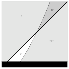
Figure 2: The phase space of the single string system that comes from the Hagedorn dominance rule (40) and the winding excitation energy $E_{\omega}$

Suppose the system we are interested has $DD-a$ Dirichlet dimensions compactified at radius $R_{DD}$, while the purely Neumann and $a$ Dirichlet ones are already open.

If $E_{H}\ll E_{\omega}\ll E$ the winding states are excited when the Hagedorn term of the density of states clearly dominates the dynamics of the system. As a consequence the winding influence could be neglected. In this case the thermal behavior of the single string is accounted by the first term of (35) with $\tilde{D}=NN+DD-a$. This is in fact the situation in which the radius of the $DD$ direction is small and could be better treated by tacking advantage of $T$-duality converting the $DD$ directions into $NN$ ones. In the figure this regime correspond the region $I$.

In the case in which $E_{H}\ll E\ll E_{\omega}$, the region $II$ of the picture, we have a system that effectively lives in a space without the $DD$ directions and whose thermodynamics is governed by the Hagedorn term. The density of states in this case is the leading term of (36). However the existence of this region is closely related to the value of the cut-off $\Lambda^{2}$, and appears at energies $E\sim E_{c}$, so we think that it must be studied by the IR regular density of states.

We can go now to the region $III$ in which $E\ll E_{H}\ll E_{\omega}$. This region behaves exactly in the same way as the region $II$, but the difference comes from the fact that it appears for every value of the cut-off $\Lambda^{2}$. On the other hand it must be described by the high energy density of states in an $a$-dimensional background.

Finally we must look to the region $IV$. It corresponds to $E_{\omega}\ll E\ll E_{H}$. In this case all the terms of (35) are relevant. We think that it would be better accounted with a complete density of states, overall when going to the multiple string system. The advantage of the asymptotic expression over the exact one, that is simplicity, is lost and it is better to use the complete series.

We would like to make two final comments on the thermodynamics at high energies. It is interesting to note that if we pass from the region $III$ to the $I$ of the phase space, by increasing the energy of the system, it could test large extra dimensions. Then by this mechanism we can change the dimensionality if the background in which the system is evolving.

On the other hand it seem remarkable to us that there are some target background in which by this transition, we pass from a system which has a negative specific heat to another one with a positive and finite specific heat and which asymptotically ends at the Hagedorn temperatures. In terms the nomenclature of [18] we go from a non-limiting case to a limiting one.

Finally we would like to mention how these densities of states could apply for the multiple string gas. Using the convolution description of [8] we know that the multiple string gas density of states is obtained as

$$\Omega(E)=\sum_{N=0}^{\infty}\frac{1}{N!}\,\Omega^{(1)}(E)\star\cdots\star\Omega^{(1)}(E)$$ (44)

where the stars stand for convolution integrals. One of the possible approximations at high energy that we can do for the density of states of the $N$-string gas is to consider it as behaving as a single long string. If we use this picture we arrive at

$$\frac{1}{N!}\,\Omega^{(1)}(E)\star\cdots\star\Omega^{(1)}(E)\rightarrow\frac{1}{N!}\left(A\frac{V^{NN}}{V^{DD}}\right)^{N}\Omega^{(1)}(E)$$ (45)

where $A$ is a factor that must be computed for each case. The simplest one are those in which the single string is Hagedorn dominated, and we finally obtain an ultra-high energy density of states as

$$\Omega(E)\simeq\frac{e^{\beta_{H}E+A\frac{V^{NN}}{V^{DD}}}}{E^{(9-\tilde{D}-\nu)/2}}{\cal H}\left(E-E_{c}\right).$$ (46)

It corresponds to the leading order in the computation of [7, 18] and the corrections come from the series of $\Omega^{(1)}(E)$. The thermal behavior of the multiple string system exactly matches with the single string one with the previous assumption, as for $\Omega_{1}(E)$ it does not work in the IR region. We finally conclude that only a complete computation of the single string density of states can be trusted for the multiple object gas.

5 The Complete Density of States

In what follows we will obtain the complete density of state for the single string and use it to describe the string gas thermodynamics. The idea here is to try to inverse Laplace transform the whole free energy of the open string gas. The method that we will follow was presented in [8]. We write the free energy of the open string theory as

$$-\beta F(\beta)=-(2\alpha^{\prime})^{-(NN+DD+1)/2}\frac{V^{NN}}{V^{DD}}\frac{\beta}{4\pi}\sum_{\{M\}}\int_{0}^{\infty}\frac{dt}{t}t^{-(NN+DD+1)/2}e^{-\frac{\pi}{2t}M^{2}}f(t).$$ (47)

where the internal partition function is taken as in (22). The parameter $M^{2}$ is the mass of the closed string boundary states propagating between the branes with the Euclidean time compactified on a circle of length $\beta$. It is given by

$$M^{2}=\frac{1}{\alpha^{\prime}}\left[\sum_{i}^{NN}n_{i}^{2}R_{i}^{2}+\sum_{i}^{DD}\frac{m_{i}^{2}}{R_{i}^{2}}+\frac{\beta^{2}}{4\pi^{2}}(n+1/2)^{2}\right].$$ (48)

At this moment we need to express the internal partition function as a sum over open string states. More concretely we want to explicitly write

$$f(t)=\sum_{k=0}^{\infty}a_{k}\,e^{-m^{2}_{k}t}\hskip 14.22636pt\mbox{with}\hskip 14.22636pta_{k}=\frac{1}{2\pi i}\oint\frac{dq}{q^{k+1}}f(q).$$ (49)

Including the previous Taylor expansion and the parameter $\nu$ in (47), we can finally write

$$-\beta F(\beta)=-(2\alpha^{\prime})^{-(NN+DD+1)/2}\frac{V^{NN}}{V^{DD}}\frac{\beta}{4\pi}\sum_{\{M\}}\sum_{k=0}^{\infty}a_{k}\int_{0}^{\infty}\frac{dt}{t}t^{-(10-\nu)/2}e^{-\frac{\pi}{2t}M^{2}}e^{-k\pi t}.$$ (50)

By using the integral representation of the Bessel functions $K(z)$ we can express the Helmholtz Free Energy of the open string gas as a sum over the Free Energies of each target massive fields in the following way

$$-\beta F(\beta)\sim-\frac{V^{NN}}{V^{DD}}\frac{\beta}{2\pi}\sum_{\{M\}}\sum_{k=0}^{\infty}a_{k}(k\pi)^{\frac{10-\nu}{2}}K_{\frac{10-\nu}{2}}\left(\pi M\sqrt{2k}\right)\left(\pi M\sqrt{\frac{k}{2}}\right)^{\frac{\nu-10}{2}},$$ (51)

where the constant in front of the integral (47) have been ignored.

At this moment we would like to obtain the single string density of states by the inverse Laplace transformation of the Free Energy in (51) as it was done in [8]. The complicate dependence of the argument of the Bessel function on the compactification parameters, the radii $R$, and on the inverse temperature $\beta$, makes this computation hard. We will attempt it by a simple trick, that however seems useful to study some interesting and simpler limit before.

Let us begin with the study of the decompactification limit that corresponds to taking all the radii to infinity. In this background the relevant degrees of freedom would correspond to the momenta in the $NN$ directions. As we discussed in section 3 this is the only way to completely avoid the winding contribution. It is due to the fact that we can forget about the winding states for the single string by taking its energy smaller than the squared Dirichlet radius $R_{DD}$, but in order to do the same for the multiple string gas we must prevent the statistical fluctuations that could allow a winding nucleation. The density of energy is finally constrained to be in a low range of values by (39). In summary, the correct way to study the system in absence of winding states consists of taking the radius of the $DD$ direction to infinity and not to assume string energies lower than the winding masses.

We take the desired limit in (21), by assuming the $NN$ momenta to have a continuous spectrum and taking only into account the winding zero mode we arrive at

$$-\beta F(\beta)\sim-V^{NN}\frac{\beta}{2\pi}\sum_{n\in{{Z}}}\sum_{k=0}^{\infty}a_{k}(k\pi)^{\frac{NN+1}{2}}K_{\frac{NN+1}{2}}\left(\pi M_{n}\sqrt{2k}\right)\left(\pi M_{n}\sqrt{\frac{k}{2}}\right)^{-\frac{NN+1}{2}},$$ (52)

where the masses now are reduced to

$$M_{n}=\frac{\beta|2n+1|}{4\sqrt{\alpha^{\prime}}\pi}.$$ (53)

The density of states corresponding to this free energy can be obtained by using exactly the same method of [8], getting the following result

$$\Omega^{(1)}(E)=\frac{2V^{NN}(4\pi)^{\frac{NN}{2}}}{\Gamma(\frac{NN}{2})}\sum_{n=odd}\sum_{k=0}^{\infty}a_{k}n^{-(NN+1)}E\left(E^{2}-\frac{n^{2}k}{8\alpha^{\prime}}\right)^{\frac{NN}{2}-1}{\cal H}\left(E^{2}-\frac{n^{2}k}{8\alpha^{\prime}}\right).$$ (54)

We can compare the high energy density of states for the single string system in the open universe case, that corresponds to the result expressed in (36). The crucial difference comes from the IR behavior. The expression in (54) is regular at low energies because we did not exclude out any mass levels of the string, as we did for the first case, by using $\Lambda^{2}$. The critical Hagedorn phenomenon here is hidden in the growth of the coefficient $a_{k}$, and appears as the energy is big enough to open massive string thresholds.

We can compute the density of states for the string gas living in a universe with compact dimensions. The way of computing it is the same we have used above. In this case the free energy is represented by the $K_{1/2}(z)$ Bessel function. The trick that we will use here to use the result of [8] and obtain the density of states consists of writing the free energy in (47) as

$$-\beta F(\beta)=-(2\alpha^{\prime})^{-(NN+DD+1)/2}\frac{\beta}{4\pi}\sum_{n=0}^{\infty}\sum_{\{M_{knw}\}}\int_{0}^{\infty}\frac{dt}{t}t^{-1/2}e^{-\frac{\beta^{2}}{8\pi t}(n+1/2)^{2}}e^{-\frac{2\pi}{\alpha^{\prime}}M_{knw}^{2}}$$ (55)

where the mass threshold here are expressed in terms from the open string side as

$$M_{knw}^{2}=\sum_{i=1}^{NN}\frac{4n_{i}^{2}}{R_{i}^{2}}+\sum_{j=1}^{DD}4w_{j}^{2}R_{j}^{2}+2\frac{\pi}{\alpha^{\prime}}^{2}k.$$ (56)

The case in which all the dimensions are compact and their radii are small enough to force us to consider the spectrum of momentum and winding strongly discretized, is very subtle. We will then begin with the case in which we assume that the $NN$ direction are open and the $DD$ ones are compactified before. The density of states in this case is

$$\Omega_{(1)}(E)=\frac{2V^{NN}(4\pi)^{\frac{NN}{2}}}{\Gamma(\frac{NN}{2})}\sum_{n=odd}\sum_{M_{kw}}^{\infty}a_{k}n^{-(NN+1)}E\left(E^{2}-\frac{n^{2}M_{kw}}{16}\right)^{\frac{NN}{2}-1}{\cal H}\left(E^{2}-\frac{n^{2}M_{kw}}{16}\right).$$ (57)

where the string masses now are related to the winding number only

$$M_{kw}^{2}=\sum_{j=1}^{DD}4w_{j}^{2}R_{j}^{2}+2\frac{\pi}{\alpha^{\prime}}^{2}k.$$ (58)

With this density of state is very easy to study the case in which the single string cannot probe some $DD$ direction. It is simply accounted by taking some of the winding radii to infinity, another important feature is that the IR validity of it allows us to study the multiple string gas and then we would be able to analyze the possibility of defining some effective dimensions and the existence of energy density scales that probe extra large compactified directions.

Finally we are able to obtain the density of states, for the a null number of non-compact $NN$ dimensions. It corresponds to

$$\Omega^{(1)}(E)=\frac{2}{\Gamma(\frac{0}{2})}\sum_{n=odd}\sum_{M_{knw}}^{\infty}a_{k}n^{-1}{\cal\delta}\left(E-\frac{n\,M_{knw}^{1/2}}{4}\right)$$ (59)

The first noticeable feature of this result is that we do not have any continuous dependence on the energy. The density of states above strictly corresponds to the degeneracy of each mass level without any kinematical contribution. On the other hand we know that by $T$-dualizing the $NN$ directions we can describe the system of wrapped D-branes as a system of D-particles on a torus. It is interesting to note that if we take the radii of the $DD$ direction to infinity we arrive at a system of D0-branes in an already open target space. In this case the density of states is reduced to a sum of the mass degeneracy times the Dirac-delta function located at each mass level.

Two relevant limits of this result should be analyzed. If we take the energy to be large one we should arrive at a result related to the exponential growth of the degeneracy of string mass levels. Doing it in (59) we in fact arrive at

$$\Omega^{(1)}(E=m)\sim e^{\beta_{H}m}\,m^{-9/2}{\cal H}\left(m-\frac{2\pi}{\beta_{H}\Lambda^{2}}\right),$$ (60)

that corresponds to the leading term of (36) and to the critical behavior studied in the early works on the subject [1, 2]. As we mention before, because of the absence of any kinematical degrees of freedom, the energy here is exactly the mass of the strings. What is remarkable is that once again the cut-off establish the range of validity of the approximation.

On the other hand it is interesting to relate the previous result to the SYM description of the D-brane thermodynamics [10, 11, 12] and more concretely to the finite temperature behavior of Matrix model of M-theory [19, 20]. Taking the massless limit of the open string theory on the brane we arrive to the SYM description of the system. On the microcanonical side this is implemented by simply taking into account the first term of the density of states above. It finally gives a constant density of states that equals the polarization of the massless string modes times a delta at zero energy. We can obtain the same result by firstly starting by the canonical free energy of the SYM₀₊₁ theory. It reads

$$F(\beta)\sim\beta^{-1}\sum_{n=odd}^{\infty}n^{-1}.$$ (61)

If we make the inverse Laplace transformation of $Z^{1}(\beta)=-\beta F(\beta)$, we easily see that the single-object density of states $\Omega^{(1)}_{SYM}(E)$ exactly matches the massless limit of our result in (59).

One final comment. The density of states in (59) has the divergent $\Gamma(\frac{0}{2})$ in the prefactor. The value of this function makes the density of states vanish and this needs some interpretation. What is happening is that, because of the compactness of the background universe, the spectrum of the string mass is discrete. This means that in a given energy range there could be isolated accessible states only, in such a way that we cannot define a density of states. In our computation we have supposed the spectrum to be continuous and we recover a vanishing $\Omega^{(1)}$ for the single string. In principle thermodynamics is not affected because, in the microcanonical ensemble, the physical magnitudes come from the derivatives of the entropy, which is proportional to the logarithm of the density of states, so we can anyway neglect any multiplicative constant.

6 The number of strings and the entropy.

In [8, 9, 6, 7, 14] a picture was studied for the phase transition occurring at the Hagedorn temperature. The transition signal was the appearance of a fat string that breaks equipartition and absorbs enough energy to excite high mass levels while all the others remain massless and form a kind of background, that we called ’the sea’ [8, 9]. We would like now to see how the number of strings evolves and how the sea and the fat string share the energy as the volume varies. To study that, we approximate the high-energy density of states by

$$\Omega_{High}(E,E_{sea},V)=V(E-E_{sea})^{-\frac{a}{2}}e^{\beta_{H}(E-E_{sea})}\Omega_{sea}(E_{sea})$$ (62)

with

$$\Omega_{sea}=\frac{1}{\Gamma(dN)}\frac{1}{N!}\left(\frac{\Gamma(d)\zeta(d+1)(d-1)^{2}}{2^{d-1}\pi^{d/2}}f(V)\right)^{N}E_{sea}^{dN-1}$$ (63)

where $a$ is a constant integer that depends on the model and the D-brane background, $d$ is the number of open dimensions (testable and continuous at low energies), $N$ is the number of strings and $E_{sea}$ is the mean energy of the sea. We can use concepts like average energy in spite of working with the microcanonical ensemble because we have separated our microcanonical system into two parts. Each possesses a thermodynamical (physically infinite) number of degrees of freedom so that they act as an ’Energy reservoir’ for the other. That is, the sea of massless strings can be thought of as a gas in the canonical ensemble. Throughout the following calculation we shall ignore the thermal fluctuations, so that we shall suppose that the energy or the volume are large enough.

Firstly, we calculate how the energy is shared between both subsystems. The most probable distribution is given by the following equation:

$$\left.\frac{d\Omega_{High}}{dE_{sea}}\right|_{E,V}=0$$ (64)

The solution to it is

$$E_{sea}=\frac{dN}{\beta_{H}},$$ (65)

each light string having an average energy $d/\beta_{H}$, which is the energy at which the massless fields reach the Hagedorn temperature in $d$ spatial dimensions. This result was already obtained in [8] using a model of kinetic theory.

This is part of the equation of state and it allows us to write

$$\Omega_{High}(E,E_{sea},V)=\Omega_{High}(E,N,V).$$ (66)

This form of the density of states permits to calculate the most probable average number of strings for given values of the total energy and the volume and therefore, how the energy is shared between the two subsystems. The equation is:

$$\left.\frac{d\Omega_{High}}{dN}\right|_{E,V} = 0$$

$$E_{fat}=\left(E-\frac{dN}{\beta_{H}}\right) = \frac{da}{2\beta_{H}}\left[-1-log\left(\frac{\Gamma(d)\zeta(d+1)(d-1)^{2}}{2^{d-1}\pi^{d/2}N}f(V)\right)\right]^{-1}$$ (67)

For certain values of $V$ and $N$ the energy of the fat string becomes small or even negative, that is, it ceases to exist. This gives a critical value for $f(V)$ that separates two phases with and without the fat string. The phase without fat string is easy to analyze because the main contribution comes from the massless string gas. Its density of states is

$$\Omega(E,V)=\sum_{N=0}^{\infty}\frac{1}{\Gamma(dN)N!}\left(\frac{\zeta(d+1)\Gamma(d)(d-1)^{2}}{2^{d-1}\pi^{d/2}}\right)^{N}V^{N}E^{dN-1}$$ (68)

For large volumes and energies, it yields

$$T=\frac{1}{d}\epsilon$$

$$\epsilon=d\left(\frac{2^{d-1}\pi^{d/2}}{\zeta(d+1)\Gamma(d)(d-1)^{2}}\right)^{\frac{1}{d}}\rho^{\frac{1}{d}}$$ (69)

where

$$\epsilon=\frac{E}{<N>}$$

$$\rho=\frac{<N>}{V}$$ (70)

The subsequent analysis of this expressions depends on the particular form of $f(V)$. In the case of closed strings it is $V+1/V$, that tends to $V$ away from the selfdual volume. Besides, $d$ equals $9$ and $a$ equals $1/2$. As a result, equation (67) gives a critical value of $\rho_{crit}\simeq 159$ strings per $\alpha^{\prime 9/2}$. If we now take the thermodynamical limit ($V$ and $E$ $\rightarrow\infty$) $N$ dynamically diverges maintaining the densities finite. As both densities, $\rho$ and $\epsilon$, grow together, any of them can be taken as the only parameter defining the system. The physical picture is as follows: If the density is lower than the critical one, the system behaves like a massless gas in ten dimensions and the temperature grows linearly with $\epsilon$. When the density reaches the critical value a phase transition occurs and, as the correlation length tends to infinity, the system tends to concentrate the energy on one fat string with infinite mass. Beyond the transition point, the energy of the fat string becomes finite and decreasing with the density. The finiteness of $E_{fat}$ drive us to formally say that its ’Energy density’ is zero. We use the inverted commas because one can hardly talk about a density for a single object but this is quite a peculiar one because it has influence over global properties. Its rôle is to regulate the temperature so that the bath always remains at $T_{H}$. The system prefers to create more and more light strings rather than exciting higher massive modes of the already existing ones.

The evolution of the temperature is singular. At low energies, the temperature grows with increasing specific heat. At the critical point, the temperature is $T_{H}$ and remains so thereafter with infinite specific heat. This is a confirmation of the image depicted in [8]. Fig.(5) shows the qualitative behavior.

The case of open strings attached to D-branes is quite different because

$$f(V)=\frac{V_{NN}}{V_{DD}}.$$ (71)

The transition depends on how we take to infinite both volumes. If

$$\frac{V_{NN}}{V_{DD}}\rightarrow\infty$$ (72)

the analysis is identical to that of closed strings, but defining a new density

$$\rho=\frac{NV_{DD}}{V_{NN}}$$ (73)

It is the density of strings one would define in the T-dual theory where all the directions have Neumann boundary conditions. Other possible limit is the opposite one

$$\frac{V_{NN}}{V_{DD}}\rightarrow 0$$ (74)

which is equivalent to taking $\rho$ to infinite. The energy of the fat string tends to zero but is still acts as a regulator so that there is an equilibrium between an unstable fat string and the sea that fills the space at $T_{H}$.

There is one exceptional case when $a=0$, that is, for open strings in a completely testable universe. In that case, the breaking of equipartition is quite peculiar. Compare figs. (3) and (4). There is never a sharp peak in the density of states of several strings signaling the most probable appearance of a fat one that absorbs much more energy than the others. Rather, there is a spread in the probability that means that the fluctuations in the energy of a single component are comparable to the total energy. This invalidates the physical image of the single string dominance of thermodynamics and even prevents the correction of it due to what we have called the sea. The correct physical image is a gas where equipartition more or less holds but with very large fluctuations in the energy of particular strings. This makes the need for the exact calculation stronger because the probability of finding a string in virtually any point of the phase space is large. The only prediction that can be obtained with the asymptotic expressions is that the asymptotic temperature is Hagedorn and that the specific heat is always positive.

This is the only case in which there is not a phase transition if we take the appearance of the fat string as the order parameter. However, at energy densities beyond the Planck scale, the system acquires a rather anomalous behavior. For the moment, we cannot precise if it corresponds to a higher order phase transition or simply a soft change of behavior.

The difference between the usual microcanonical point of view and this one is the fact that here we are letting the number of strings dynamically vary, that is, we are working in the ($E$, $V$, $\mu$)-ensemble instead of the pure microcanonical. The former is more adapted to the string gases because they naturally have a fixed and null chemical potential. Somehow, it is a way to gather the different descriptions in terms of finite-$N$ gases together. As explained in sections $4$ and $5$, one can make convolutions of the single string density of states and obtain the behavior of different subsystems with a fixed number of constituents. The ($E$, $V$, $\mu$)-ensemble shows us how the transition between them happen.

Figure 3: Probability of the energy distribution for 2-string system in the $\nu=6$ case, at high energies.

The inclusion of the sea as an important contribution to thermodynamics has consequences on the estimation of the entropy. One has to add the logarithm of (62), that is, in the large-$N$ limit

$$S(V,E,N)=log\Omega(V,E,N)=10N+Nlog\frac{CVE^{9}}{9^{9}N^{10}}$$ (75)

where $C$ is a constant. Substituting the value of $N$ that solves the equation of state (69), it is

$$S(V,E)=10N=\frac{10}{9}\rho V=\frac{10}{9}\left(\frac{\epsilon}{9}\right)^{9}V$$ (76)

This is the leading contribution except when $a=0$.

Let us now write about the pressure. The density of states that we have obtained in the previous section has the functional form:

$$\Omega(V,E)=f(E)\times g(V)$$ (77)

where

$$g(V)=\frac{V_{NN}}{V_{DD}}$$ (78)

This means that the dependence of the pressure on the temperature is the same as that of the free energy. However, its dependence on the volume is not trivial at all. Let us recall that, in traditional theories

$$P=\left.-\frac{\partial F}{\partial V}\right|_{T}.$$ (79)

However, we know that T-duality is an exact symmetry in type II String Theory. This means [9] that every physical (measurable) magnitude must be invariant under T-duality. This, of course, includes the pressure. The usual definition, that we have written just above, is not T-selfdual and therefore it must be corrected and substituted with another. We shall use the proposal in [9].

$$P=\left.-\frac{\partial F}{\partial V}\right|_{T}{\cal H}\left(V-\alpha^{\prime\tilde{D}/2}\right)-\left.\frac{\partial F}{\partial(1/V)}\right|_{T}{\cal H}\left(\frac{1}{V}-\alpha^{\prime\tilde{D}/2}\right)$$ (80)

This case is even more complicated because the function we are interested in is not homogeneous in the volume, so the derivative must be decomposed as

$$V=\prod_{i=1}^{\tilde{D}}(2\pi R_{i})$$

$$dV=\sum_{i=1}^{\tilde{D}}\frac{V}{R_{i}}dR_{i}$$ (81)

$$\frac{\partial}{\partial V}=\sum_{i=1}^{\tilde{D}}\frac{R_{i}}{V}\frac{\partial}{\partial R_{i}}$$

and

$$P=\sum_{i=1}^{\tilde{D}}\left[\left.-\frac{R_{i}}{V}\frac{\partial F}{\partial R_{i}}\right|_{T}{\cal H}\left(R_{i}-\alpha^{\prime 1/2}\right)\left.-\frac{1}{VR_{i}}\frac{\partial F}{\partial 1/R_{i}}\right|_{T}{\cal H}\left(\frac{1}{R_{i}}-\alpha^{\prime 1/2}\right)\right]$$ (82)

with this, and if we assume that all $R_{i}$ are larger than $\alpha^{\prime}$,

$$\frac{d}{dV}\frac{V_{NN}}{V_{DD}}=\frac{1}{V_{DD}^{2}}(NN-DD).$$ (83)

It is interesting to see what happens when we make T-duality act on the free energy so that, for example, all the directions are Neumann, the result would be

$$\frac{d}{dV}V_{NN}^{\mbox{\tiny T-dual}}=(NN-DD),$$ (84)

where $NN$ and $DD$ are the original Neumann and Dirichlet dimensions. The result is similar up to a multiplicative constant term. In fact one can see that what really coincides in both points of view of the same theory is the product

$$PV\propto(NN-DD)\frac{V_{NN}}{V_{DD}}$$ (85)

One remarkable characteristic of the pressure we have calculated is that, in certain cases, it vanishes. This happens whenever the number of directions with Neumann and Dirichlet boundary conditions coincide. This is only possible if an odd number of dimensions is untestable.

Figure 4: Probability of the energy distribution for 2-string system in the $\nu=0$ case, at high energies.

7 Conclusions

In this paper we have studied the thermal behavior of string systems in D-brane backgrounds in the microcanonical ensemble. The goal of this kind of analysis is to delucidate what is the rôle of the Hagedorn temperature in the thermodynamics of Dirichlet open string theories. As in the closed string cases the necessity of the microcanonical description comes from the breaking of the canonical ensemble at Hagedorn temperatures.

Our strategy has been as follows, and is along the lines of [8, 9]. We have begun by a computation of the asymptotic density of states of the single string. These computation are analogous to those of [6, 7] for the closed-string gas and have been recently used for the D-brane cases in [18]. We have shown that this procedure corresponds to including an IR cut-off $\Lambda^{2}$ that eliminates the contribution of the massless string modes. Consequently the densities of states obtained are not valid for the low energetic regime. We have studied the range of validity of this approximation in terms of the energy of the system, the radii of the compact dimensions and the value of $\Lambda^{2}$. The result is a kind of phase space where different parts are best described by particular approximations. Only two of these parts are well described by the asymptotic density of states, approximated by the Hagedorn term only. Passing from one of them to the other the number of effective dimensions of the target space the string gas lives on changes. We claimed that in order to completely know the thermal behavior it is necessary to use a complete, IR regular density of states.

On the other hand the thermodynamics of the string gas is not exactly described by the single string system, so we need to study the multiple string density of states. We should follow the convolution prescription of [8]. However it is not possible to do it using the high energy densities of states of the single string because of their irregular IR behavior. Finally one is lead to look for a complete density of states.

Before computing the desired density of states we have analyzed the thermal properties of the single string. We have shown that there is a negative specific heat phase in all cases except for the $\tilde{D}+\nu=9$ one. In the latter we have an IR definite phase but we think that at these energies the density of states does not include all the information. It is in fact obvious that the corrections to the leading behavior are strongly dependent of $\Lambda^{2}$,and that way nothing warrants that we are including all the IR degrees of freedom of the theory. The only extractable conclusion is that after including all the IR information we will still have a positive specific heat phase, and Hagedorn will be a asymptotic maximum temperature of the system.

We have calculated an exact expression for the single string density of states in section 5. It is got in the form of a series with a finite number of terms for finite values of the energy. The results are analogous of those in [8, 9]. With those instruments, we are able to study the thermodynamics of the systems and also to match our results with those obtained using the SYM_p+1 description of the D-branes dynamics. We have used the $\tilde{D}+\nu=9$ cases as some special examples. In one of them, $DD=9$, we are able to connect with the Matrix model microcanonical description, in the Born-Oppenheimer approximation.

In particular, we study the distribution of energy among the constituents. This gives us physical images that help us test models that had been proposed in earlier works [8, 9, 6]. When a fat string with more energy than the rest appears and, therefore, equipartition is broken, a phase transition occurs. We have been able to distinguish the cases in which this happens and in which it does not. We have seen how this affects the temperature and the specific heat value, the case in which the phase transition occurs has been plotted in Fig.(5). When several of this systems are put in thermal contact, that is, when open strings attached to different D-branes and free closed strings thermally interact, the behavior of the global system is dominated by the most degenerate phase. This is the one that gives lower temperature and smaller specific heat for a value of the energy: open strings with $\tilde{D}+\nu=9$. A similar picture has already been obtained in [18]; the difference between our picture and theirs is that in ours all subsystems have $T_{H}$ as the maximum temperature. There is not any ’non-limiting’ system with temperatures higher that $T_{H}$. Our result is that systems can be classified between those with phase transition and those without it. The systems without phase transition are the closed strings in a completely compactified space [9] and open strings with $\tilde{D}+\nu=9$. Whenever there is at least one open direction, the only system that does not suffer phase transition is that of open strings with $\tilde{D}+\nu=9$. When one considers the whole system made up with closed strings and open strings of various types (various values of $\nu$,$DD$ and $NN$), the most degenerate system dominates the thermodynamics. It is always the one without transition. This means that the existence of one D-brane prevents any phase transition, except when some $DD$ are open.

Along all these considerations we have considered all the untestable $DD$ direction to be already open. If we had not done it we would have found some of the previous systems in thermal contact having the phase transition. It corresponds to systems that stand in region $III$ of fig.(2). This systems have the energy per string ($\rho_{N}$) constraint by (39). On the other hand we know that the phase transition occurs at $E/N\sim\tilde{D}\,T_{H}=\rho_{H}$. Two possibilities come. If $\rho_{H}<\rho_{\omega}$ the systems suffers a phase transition. Else we need to include all winding states and finally we pass to the region $I$ where we do not find any phase trasition. We think that in the thermodynamic limit, where $\rho_{\omega}$ goes to zero, a phase transition is prevented.

Figure 5: Temperature versus energy for the multiple string systems that reach Hagedorn temperature through the long string nucleation

Regarding the pressure, we calculate it in several cases and see the peculiarities of string systems using the String-Theory definition of it proposed in [9].

Finally, we use the ’fat string-sea’ model to make a calculation in a genuinely thermodynamic limit, and see the evolution of the temperature as a function of string and energy densities instead of absolute magnitudes.

8 Acknowledgments

We thank a lot M. A. R. Osorio for enlightening and very helpful discussions and J. L. F. Barbón for useful comments. The work of M. L. M. was partially supported by MEC under a FP-97 grant.

References

- [1] R.Hagedorn Nuovo Cimento Supp.3 147 (1965)
-
[2]
S.Frautschi Phys. Rev. D3(1971)2821
R.Carlitz Phys. Rev. D5(1972) 3231
N.Cabbibo and G.Parisi Phys. Rev. B59(1975)67 - [3] E.Álvarez Nucl.Phys. B269 (1986)596
- [4] E.Álvarez and M. A. R. Osorio, Phys. Rev. D36(1987)1175
- [5] M.J. Bowick and S.B. Giddings, Nucl.Phys. B325 (1989)631 S.B. Giddings, Phys.Lett. B226 (1989)55
- [6] N.Deo, S.Jain and C.-I.Tan Phys. Rev. D45(1992)3641
-
[7]
N.Deo, S.Jain and C.-I.Tan Phys. Rev. D40(1989)2626
M.Axenides, S.D.Ellis and C.Kounnas Phys. Rev. D37 (1988)2964
M.McGuigan Phys. Rev. D38(1988)552 - [8] M. Laucelli Meana, M. A. R. Osorio, and J. Puente Peñalba, ”The String Density of States from The Convolution Theorem”, Phys. Lett. B400(1997)275, hep-th/9701122
- [9] M. Laucelli Meana, M. A. R. Osorio, and J. Puente Peñalba, ”Counting Closed String States in a Box”, Phys. Lett. B408(1997)183, hep-th/9705185
- [10] M.B.Green, ’Wilson-Polyakov loops for critical strings and superstrings at finite temperature’ Nucl.Phys. B381 (1992)201; ’Temperature Dependence of String Theory in the Presence of World-Sheet Boundaries’ Phys. Lett. B282(1992)380, hep-th/9201054
- [11] M. A. Vazquez-Mozo, ’Open String Thermodynamics and D-Branes’,Phys. Lett. B388(1996)494, hep-th/9607052
- [12] A. Tseytlin ”Open superstring partition function in constant gauge field background at finite temperature”, hep-th/9802133
- [13] J. L. F. Barbon and M. A. Vazquez-Mozo,’Dilute D-Instantons at Finite Temperature’,Nucl.Phys. B497 (1997)236, hep-th/9701142
-
[14]
D.A. Lowe and L. Thorlacius, ’Hot String Soup’,Phys. Rev. D51(1995)665, hep-th/9408134
S. Lee, L.Thorlacius,’Strings and D-Branes at High Temperature’, Phys. Lett. B413(1997)303, hep-th/9707167 - [15] J.Polchinski,’TASI Lectures on D-Branes’,hep-th/9611050
- [16] D. Amati, J.Russo, ’Fundamental Strings as Black Bodies’, hep-th/9901092
- [17] K. R. Dienes, E. Dudas, T. Gherghetta, A. Riotto, ’Cosmological Phase Transitions and Radius Stabilization in Higher Dimensions’, hep-ph/9809406.
- [18] S. A. Abel, J. L. F. Barbon, I. I. Kogan, E. Rabinovici, ’String Thermodynamics in D-Brane Backgrounds’, hep-th/9902058.
-
[19]
U. H. Danielsson, G. Ferretti and B. Sundborg,
”D-particle Dynamics and Bound States”, Int. J. Mod. Phys.A11(1996)
5463-5478, hep-th/9603081.
D. Kabat and P. Pouliot, ”A Comment on Zero-brane Quantum Mechanics”, Phys. Rev. Lett.77 (1996) 1004-1007, hep-th/9603127
T. Banks, W. Fischler, S. H. Shenker and L. Susskind, ”M Theory As A Matrix Model: A Conjecture”,Phys. Rev.D55 (1997) 5112-5128, hep-th/9610043. -
[20]
N.Ohta, J.Zhou. ’Euclidean Path Integral, D0-Branes and Schwarzschild
Black Holes in Matrix Theory’
Nucl.Phys. B522 (1998) 125-136, hep-th/9801023
M. Laucelli Meana, M. A. R. Osorio, and J. Puente Peñalba, ”Finte Temperature Matrix Theory”, Nucl.Phys. B531 (1998)613, hep-th/9803058
B.Sathiapalan, ”The Hagedorn transition and the Matrix Model of Strings” Mod.Phys.Lett.A13(1998) 2085
J. Ambjorn, Y.Makeenko, G.Semenoff, ’Thermodynamics of D0-branes in matrix theory’, Phys.Lett. B445(1999)303, hep-th/9810170,
M. Li,’Ten Dimensional Black Hole and the D0-brane Threshold Bound State’,hep-th/9901158