IFUP-TH 8/99

February 1999

Loop corrections and graceful exit

in string cosmology

Stefano Foffa^a, Michele Maggiore^a and Riccardo Sturani^b,a

(a) Dipartimento di Fisica, via Buonarroti 2, I-56100 Pisa, Italy,
and INFN, sezione di Pisa.

(b) Scuola Normale Superiore, piazza dei Cavalieri 7, I-56125 Pisa.

Abstract

We examine the effect of perturbative string loops on the cosmological pre-big-bang evolution. We study loop corrections derived from heterotic string theory compactified on a $Z_{N}$ orbifold and we consider the effect of the all-order loop corrections to the Kähler potential and of the corrections to gravitational couplings, including both threshold corrections and corrections due to the mixed Kähler-gravitational anomaly. We find that string loops can drive the evolution into the region of the parameter space where a graceful exit is in principle possible, and we find solutions that, in the string frame, connect smoothly the superinflationary pre-big-bang evolution to a phase where the curvature and the derivative of the dilaton are decreasing. We also find that at a critical coupling the loop corrections to the Kähler potential induce a ghost-like instability, i.e. the kinetic term of the dilaton vanishes. This is similar to what happens in Seiberg-Witten theory and signals the transition to a new regime where the light modes in the effective action are different and are related to the original ones by S-duality. In a string context, this means that we enter a D-brane dominated phase.

1 Introduction

Pre-big-bang cosmology has been initially developed using the lowest-order effective action of the bosonic string [1]. This allowed to understand the basic features of this cosmological model: the Universe starts at weak coupling and low curvature, follows a superinflationary evolution, and enters a large curvature phase. As long as we are in the perturbative regime, a description with the lowest order effective action is adequate, and can be used to discuss the cosmological evolution [1], the generality of the initial conditions [2], and even to develop some interesting phenomenological consequences concerning the generation of primordial gravitational, axionic, dilatonic and electromagnetic backgrounds [3]. In particular, the low frequency part of these spectra is only sensitive to the low curvature part of the evolution.

At lowest order, the cosmological evolution unavoidably reaches large curvatures and strong coupling and finally runs into a singularity. At this stage it is necessary to go beyond the lowest order effective action for understanding how string theory cures the big-bang singularity, and for understanding the matching of pre-big-bang cosmology with standard Friedmann-Robertson-Walker (FRW) post-big-bang cosmology (the so-called ‘graceful exit’ problem [4-12]). One can imagine two possible scenarios. The first is that pertubative corrections succeed in turning the regime of pre-big-bang accelerated expansion into a decelerated expansion, and at the same time the dilaton is attracted by the minimum of its non-perturbative potential. This should take place before entering into a full strong coupling regime, so that perturbative results can still be trusted.

In the second scenario the evolution proceeds toward the full strongly coupled regime. In this case one must take into account that at strong coupling and large curvature new light states appear and then the approach based on the effective supergravity action plus string corrections breaks down. The light modes are now different and one must turn to a new effective action, written in terms of the new relevant degrees of freedom. In particular, at strong coupling $D$-branes [13] are expected to play an important role, since their mass scales like the inverse of the string coupling, $\sim 1/g$ and they are copiously produced by gravitational fields [14] (see also refs. [15, 16, 17, 18] for related approaches to singularities in string theory).

In this paper we investigate how far one can go within the first scenario, analyzing a variety of perturbative string loop corrections. The motivation comes in part from the works [10, 11], where the authors discuss general properties that the loop corrections should have in order to trigger a successful graceful exit. In particular, they find that the corrections should have the appropriate sign, so to induce violation of the null energy condition (NEC), but there should also be a mechanism that at some stage turns them off, otherwise the continued violation of the NEC produces an unbounded growth in the curvature and dilaton. In ref. [11] they presented a model with loop corrections chosen ad hoc, both in the sign and in their functional form, just for the purpose of verifying explicitly on a toy model the general results of ref. [10], and they found that with appropriate choices a complete exit transition is indeed obtained. A transition to a regime of decreasing curvature was also obtained, with a potential chosen ad hoc, in the second paper of ref. [1]. This shows that string loops can in principle trigger a complete graceful exit, but leaves open the question of whether this actually happens for the corrections derived from at least some specific compactification of string theory. In particular, the results of refs. [10, 11] show first of all that the corrections should have the appropriate sign, and this already is an interesting point to check against real string derived corrections, and furthermore they should also have a rather non-trivial functional form that suppresses them at strong coupling.

String loop corrections have been much studied in the literature, especially for $Z_{N}$ orbifold compactifications of the heterotic string [19-34], and we can therefore ask whether, at least in some compactification scheme, they fulfill the non-trivial properties needed for a graceful exit. In particular, corrections to the Kähler potential are known at all loops; this will be very important for our analysis, since in order to follow the cosmological evolution into the strong coupling regime, a knowledge of the first few terms of the perturbative expansion is not really sufficient, and one must have at least some glimpse into the structure at all loops.

After discussing how far one can go within a perturbative approach, we will be able to shed some light on the question of whether perturbative string theory is an adequate tool for discussing string cosmology close to the big-bang singularity, or whether instead non-perturbative string physics plays a crucial role, as in the scenario discussed in ref. [14].

The paper is organized as follows. In sect. 2 we discuss the effective action of the heterotic string with $\alpha^{\prime}$ and loop corrections for a $Z_{N}$ orbifold compactification. In sect. 3 we use these corrections to study the cosmological evolution; we will introduce various corrections one at the time, to understand better their role, and we will find solutions that, in the string frame, smoothly interpolate between the pre-big-bang phase and a phase of decelerated expansion. In sect. 4 we examine the limit of validity of the perturbative approach. We point out that loop corrections induce an instability in the kinetic term of the dilaton, that vanishes at a critical coupling. Similarly to what happens in the Seiberg-Witten model, beyond this value of the coupling the effective action is more appropriately written in terms of variables related to the original ones by S-duality. In string theory this means that there is the onset of a new regime where the light modes of the effective action are given by D-branes rather than by the massless modes of fundamental strings. Sect. 5 contains the conclusions.

2 The effective action with loop corrections

We consider the effective action of heterotic string theory compactified to four dimensions on a $Z_{N}$ orbifold, so that one supersymmetry is left in four dimensions, and we restrict to the graviton-dilaton-moduli sector. In a generic orbifold compactification there are the $(1,2)$ untwisted moduli fields $U_{i}$ and the diagonal $(1,1)$ untwisted moduli fields $T_{i}$ (non-diagonal moduli are included in the matter fields). The moduli fields $U_{i}$, determine the complex structure, i.e. the ‘shape’ of the compact space (they generalize the standard modular parameter of the torus); in various $Z_{N}$ orbifolds (see e.g. table 1 in ref. [22]) the Hodge number $h_{1,2}=0$ and therefore this shape is fixed and there are no moduli fields $U_{i}$. There are instead 3 diagonal moduli fields $T_{i}$. We will neglect the fields $U_{i}$ and we restrict to a common diagonal modulus, $T_{i}=T$; it determines the overall volume of compact space.

At the fundamental level string theory compactified on orbifolds is invariant under $T$-duality, which includes $SL(2,Z)$ transformations of the common modulus $T$

$$T\rightarrow\frac{aT-ib}{icT+d}\,,$$ (1)

with $a,b,c,d\in Z$ and $ad-bc=1$. These modular transformations are good quantum symmetries, and therefore they must be exact symmetries also at the level of the loop-corrected low-energy effective action. While at tree level the dilaton is inert under modular transformations, at one-loop the cancellation of the modular anomaly requires that the dilaton transforms as [19]

$$S\rightarrow S+2\kappa\log(icT+d)\,,$$ (2)

where Re $S=e^{-\phi}$ and $\phi$ is the dilaton field; $\kappa$ is a positive constant of order one which depends on the coefficient of the anomaly, see below. Then one easily verifies that $S+\bar{S}+2\kappa\log(T+\bar{T})$ is modular invariant. We can therefore introduce a one-loop corrected modular invariant coupling $g_{0}^{2}$ from [19, 20]

$$\frac{1}{g_{0}^{2}}=\frac{1}{2}(S+\bar{S})+\kappa\log(T+\bar{T})=e^{-\phi}+\kappa\sigma\,,$$ (3)

where we have defined the field $\sigma$ from ${\rm Re}T=(1/2)e^{\sigma}$ (the factor $1/2$ is not conventional but we found it convenient). Loop corrections to the effective action can be computed directly as an expansion in terms of the modular invariant coupling $g_{0}^{2}$ [20]. As we see from eq. (3),

$$g_{0}^{2}=\frac{e^{\phi}}{1+\kappa\sigma e^{\phi}},$$ (4)

and therefore an expansion in $g_{0}^{2}$ provides a resummation and a reorganization of the expansion in $e^{\phi}$. Note in particular that even when $e^{\phi}$ is large, the expansion in $g_{0}^{2}$ is still under control if $\kappa\sigma\gg 1$, i.e. if $\kappa\log V\gg 1$, where $V$ is the volume of compact space in string units.

We include in the action terms with two derivatives and terms with four derivatives, i.e. $O(\alpha^{\prime})$ corrections to the leading term. For both the two- and four-derivatives terms we include modular invariant loop corrections. We discuss separately the two- and four-derivatives terms in subsections 2.1 and 2.2.

2.1 Terms with two derivatives

In the Einstein frame, where the gravitational term has the canonical Einstein-Hilbert form, the action for the metric-dilaton-modulus system compactified to four dimensions is

$${\cal S}_{0}^{E}=\frac{1}{\alpha^{\prime}}\int d^{4}x\sqrt{-g}\left[\frac{1}{2}R-K_{i}^{j}\partial_{\mu}z^{i}\partial^{\mu}\bar{z}_{j}\right]\,.$$ (5)

Here $z^{i}=(S,T)$, $K_{i}^{j}=d^{2}K/dz^{i}d\bar{z}_{j}$ and $K$ is the Kähler potential. We use the conventions $\eta_{\mu\nu}=(-,+,+,+)$, ${R^{\mu}}_{\nu\rho\sigma}=\partial_{\rho}\Gamma^{\mu}_{\nu\sigma}+\ldots$ and $R_{\nu\sigma}={R^{\rho}}_{\nu\rho\sigma}$. The superscript $E$ reminds that this action is written in the Einstein frame. The Einstein-Hilbert term $\sqrt{-g}R$ is not renormalized at one-loop [26] and this non-renormalization theorem persists to all orders in perturbation theory around any heterotic string ground state with at least $N=1$ space-time supersymmetry [34]. At tree level the Kähler potential is $K_{\rm tree}=-\log(S+\bar{S})-3\log(T+\bar{T})$. It does renormalize, and at one loop, for heterotic string compactified on a $Z_{N}$ orbifold, becomes [19]

$$K_{\rm 1-loop}=-\log\left(S+\bar{S}+2\kappa\log(T+\bar{T})\right)-3\log(T+\bar{T})\,,$$ (6)

where $\kappa=3\delta^{GS}/(8\pi^{2})$. For instance for $Z_{3}$ orbifolds $\delta^{GS}=C(E_{8})/2=15$, where $C(E_{8})$ is the quadratic Casimir of $E_{8}$, and therefore $\kappa\simeq 0.57$. Eq. (6) holds at one-loop, i.e. at first order in an expansion in $1/(S+\bar{S})$. However, the all-orders resummation implicit in eq. (6) is dictated by the fact that under the modular transformations given by eqs. (1,2) the combination $S+\bar{S}+2\kappa\log(T+\bar{T})$ is invariant, and therefore respects the $T$-duality symmetry of the underlying string theory. In terms of the modular invariant coupling $g_{0}^{2}$ defined in eq. (3) we can write eq. (6) as

$$K_{\rm 1-loop}=\log\left(\frac{g_{0}^{2}}{2}\right)-3\log(T+\bar{T})\,.$$ (7)

Eq. (7) is the leading term of an expansion in $g_{0}^{2}$ of the all-order Kähler potential. Indeed, the Kähler potential has been computed at all perturbative orders in ref. [20], under the assumption that no dilaton dependent corrections other than the anomaly term are generated in perturbation theory. One defines implicitly the all-loop corrected coupling $g^{2}$ from

$$\frac{1}{g^{2}}=\frac{1}{g_{0}^{2}}+\frac{2\kappa}{3}\log(\frac{1}{g^{2}})+{\rm const.}\,\,.$$ (8)

The all-loop corrected Kähler potential then reads [20]

$$K=\log\left[\frac{g^{2}}{2}\left(1+\frac{\kappa}{3}g^{2}\right)^{-3}\right]-3\log(T+\bar{T})\,,$$ (9)

and at $g_{0}^{2}\ll 1$ it reduces to eq. (7) plus terms $O(g_{0}^{2}\log g_{0}^{2})$.

The coupling $g^{2}$ is just the effective gauge coupling that multiplies the term $F_{\mu\nu}^{2}$ after taking into account loop corrections [20] and, as we will see in the next section, it also multiplies the four derivative term. So the dilaton enters the action only through $g^{2}$. We therefore define a new field $\varphi$ from

$$g^{2}=e^{\varphi}$$ (10)

and we will treat it as our fundamental dilaton field. Therefore our loop-corrected two-derivative action is given by eq. (5) where now $z_{i}=(S^{\prime},T)$, Re $S^{\prime}=e^{-\varphi}=g^{-2}$ and $K$ is given by eq. (9).

In the following, it will be convenient to work in the string frame. In four dimensions, we define the string frame metric $g_{\mu\nu}^{S}$ in terms of the metric in the Einstein frame $g_{\mu\nu}^{E}$ from $g_{\mu\nu}^{E}=g_{\mu\nu}^{S}e^{-\varphi}$ (in four dimensions the dilaton is the same in the two frames). Note that we use $\varphi$ rather than $\phi$ to transform between the two frames. At lowest order in $e^{\phi}$ of course this reduces to the standard definition, but beyond one-loop the definition in terms of $\varphi$ is more convenient.

Writing explicitly the kinetic terms of the dilaton and modulus field, (and omitting the superscript $S$ for string frame quantities) the loop-corrected two-derivative action in the string frame reads

$${\cal S}_{0}=\frac{1}{2\alpha^{\prime}}\int d^{4}x\sqrt{-g}e^{-\varphi}\left[R+\left(1+e^{\varphi}G(\varphi)\right)\partial_{\mu}\varphi\partial^{\mu}\varphi-\frac{3}{2}\partial_{\mu}\sigma\partial^{\mu}\sigma\right]\,,$$ (11)

where we have defined

$$G(\varphi)=\left(\frac{3\kappa}{2}\right)\frac{6+\kappa e^{\varphi}}{(3+\kappa e^{\varphi})^{2}}\,.$$ (12)

2.2 Terms with four derivatives

2.2.1 The four-derivatives term at tree level

For the four derivative term we find convenient to work directly in the string frame. At tree-level it can be written as [35, 36]

$$({\cal S}_{1})_{\rm tree}=\frac{1}{2\alpha^{\prime}}\int d^{4}x\sqrt{-g}\,\left(\frac{k\alpha^{\prime}}{4}\right)\frac{S+\bar{S}}{2}\left[R_{\mu\nu\rho\sigma}R^{\mu\nu\rho\sigma}+bR_{\mu\nu}R^{\mu\nu}+cR^{2}\right]$$ (13)

and, for the heterotic string, $k=1/2$ (still, we display $k$ explicitly in our equations to make easier the comparison with ref. [8]; note however that we use the opposite metric signature compared to ref. [8]). The effective action can be obtained requiring that it reproduces the string amplitudes. This procedure fixes the coefficient of $R_{\mu\nu\rho\sigma}R^{\mu\nu\rho\sigma}$; however, the coefficients $b,c$ cannot be determined from the comparison with (on-shell) string amplitudes; this can be understood, for instance, showing that the coefficients $b,c$ do not enter in the computation of amplitudes with three on-shell gravitons, while in the computations of four-graviton amplitudes they cancel between the contact and exchange graphs [31].

A related source of ambiguity appears when one truncates the perturbative expansion in $\alpha^{\prime}$ at any finite order. In fact, suppose that we choose somehow a value for $b,c$ (two natural possibilities are either $b=c=0$ or $b=-4,c=1$, which forms the Gauss-Bonnet combination). Still, we can always perform a field redefinition that mixes different orders in $\alpha^{\prime}$, e.g. $g_{\mu\nu}\rightarrow g_{\mu\nu}+\alpha^{\prime}(a_{1}R_{\mu\nu}+a_{2}\partial_{\mu}\phi\partial_{\nu}\phi+\ldots)$, and $\phi\rightarrow\phi+\alpha^{\prime}b_{1}R+\ldots$. This would not change the physics if one would be able to include all orders in the $\alpha^{\prime}$ expansion, but it does make a difference if we truncate at a finite order in $\alpha^{\prime}$. For instance, —retaining only two- and four-derivative terms— this redefinition, applied to the two-derivative terms, generates new four derivative term, while the four-derivatives terms generates six-derivative terms which are truncated if we work at order $\alpha^{\prime}$. The terms which are generated at the four derivative level by a generic field redefinitions are just the terms $R_{\mu\nu}R^{\mu\nu},R^{2}$, plus other operators of the same order involving the dilaton, like $(\partial\phi)^{4},R^{\mu\nu}\partial_{\mu}\phi\partial_{\nu}\phi$, etc. This is another way to understand why the coeffcients of these terms cannot be fixed by the computation of string amplitudes. The term $R_{\mu\nu\rho\sigma}^{2}$ is instead unaffected by field redefinitions, consistently with the fact that its coefficient is fixed by the comparison with string amplitudes. The study of the cosmological evolution using any specific action truncated at order $\alpha^{\prime}$ should then be considered as only indicative of the possible cosmological behaviours. With suitable choices, one finds that the lowest-order pre-big-bang solutions are indeed regularized by the inclusion of $\alpha^{\prime}$ corrections, and instead of running into the singularity, they are now matched (in the string frame) to a phase of De Sitter expansion with linearly growing dilaton [8]. The effect on the cosmological evolution of these ambiguities have been studied in refs. [8, 9, 12]. Here will take the point of view that, independently of these ambiguities, a solution that, thanks to suitably chosen $\alpha^{\prime}$ corrections, approaches asymptotically a De Sitter phase with linear dilaton is a simple way to model a regularizing effect, which can have a different and deeper physical motivation: for instance, in ref. [37] we found that a similar transition to a De Sitter phase with linearly growing dilaton is driven by the formation of a gravitino-dilatino condensate. This mechanism is independent of the ambiguities discussed, and only depends on the dynamical assumption that such a condensate forms.

Our choice for the form of the tree-level-four derivative term is the same used in refs. [8, 11]:

$$({\cal S}_{1})_{\rm tree}=\frac{1}{2\alpha^{\prime}}\left(\frac{k\alpha^{\prime}}{4}\right)\int d^{4}x\sqrt{-g}\,e^{-\phi}\left[R_{\rm GB}^{2}-(\partial\phi)^{4}\right]\,.$$ (14)

In ref. [8] this form was obtained setting $b=c=0$ in eq. (13) and then performing a field redefinition that generates $R_{\mu\nu}^{2}$ and $R^{2}$ with the right coefficients to produce the Gauss-Bonnet combination $R_{GB}^{2}=R_{\mu\nu\rho\sigma}^{2}-4R_{\mu\nu}^{2}+R^{2}$, and this also generates the term $(\partial\phi)^{4}$.

Actually, our two-derivative action differs from that used in [8] already at tree level, because we have included the field $\sigma$. The field redefinition that generates the Gauss-Bonnet term will also generate a number of four-derivative terms which depends also on $\partial{\sigma}$. We will neglect these terms because, on the one hand they make the action much more complicated, and on the other hand they are basically irrelevant to the dynamics, as will be clear from the results of sect. 3 and as we have checked on some examples. Actually, because of the ambiguities intrinsic in a truncation at finite order in $\alpha^{\prime}$, it is not very meaningful to insist on any specific form of the action, and it is more important to look for properties shared at least by a large class of actions compatible with string theory.

2.2.2 The loop-corrected four-derivatives term

Let us first recall what happens in the slightly simpler case of a gauge coupling $g_{a}$, where the index $a$ refers to the gauge group under consideration. The coupling $1/g_{a}^{2}$ is identified as the coefficient of $(1/4)F_{\mu\nu}^{a}F^{a\mu\nu}$. At tree level, this term only appears when we expand in components the superfield expression $(-1/2)f_{a}(S)W^{a}W^{a}$, where $W^{a}$ is the chiral superfield containing $F_{\mu\nu}^{a}$; ${f_{a}}(S)_{\rm tree}=S$ is independent of the gauge group, and $1/g_{a}^{2}={\rm Re}S$. At one-loop $f_{a}(S)$ gets a moduli-dependent renormalization [19-34]

$${f_{a}}(S)_{\rm 1-loop}=S+\Delta_{a}(T,\bar{T})\,,$$ (15)

For orbifolds with no $N=2$ subsector, such as $Z_{3}$ and $Z_{7}$, $\Delta_{a}(T,\bar{T})=\delta_{a}$ is a moduli-independent constant, and there is no moduli-dependent one-loop correction. Beyond one-loop, $f_{a}(S)$ is protected by a non-renormalization theorem [39].

Furthermore, at one loop a contribution to $F_{\mu\nu}F^{\mu\nu}$ comes from the anomaly: in fact, since the fermions in the supergravity-matter action are chiral, the tree level effective action leads, through triangle graphs, to one-loop anomalies. The type of anomaly depends on the connections attached to the vertices. In particular, because of Kähler symmetry, chiral fermions are coupled to a $U_{K}(1)$ Kähler connection, which is a non-propagating composite field. Modular transformations are a subset of Kähler transformations and therefore, if the theory is Kähler invariant, it is also invariant under modular transformations. Considering a triangle graph with one Kähler connection and two gauge bosons attached at the vertices, we get a mixed Kähler-gauge anomaly, proportional to $F_{\mu\nu}^{a}\tilde{F}^{a\mu\nu}$. The anomaly can be represented in the effective theory with a non-local term whose (local) variation reproduces the anomaly. Because of supersymmetry, this effective non-local term, when expanded in component fields, together with $F_{\mu\nu}^{a}\tilde{F}^{a\mu\nu}$ also contains a term proportional to $F_{\mu\nu}^{a}F^{a\mu\nu}$ which, restricting to a common modulus, reads [19]

$$-\left(\frac{\kappa}{3}\right)\left[\hat{K}(T,\bar{T})-2\Box^{-1}\frac{\partial^{2}\hat{K}}{\partial T\partial\bar{T}}\partial^{\mu}T\partial_{\mu}\bar{T}\right]\frac{1}{4}F_{\mu\nu}^{a}F^{a\mu\nu}\,.$$ (16)

with $\hat{K}(T,\bar{T})=-3\log(T+\bar{T})$. In the limit of constant $T$ this term becomes local, and gives an additional moduli-dependent one-loop contribution to the gauge coupling $g_{a}^{2}$. Therefore, specializing for the moment to a $Z_{3}$ or $Z_{7}$ orbifold,

$$\frac{1}{g_{a}^{2}}=\frac{S+\bar{S}}{2}+\kappa\log(T+\bar{T})+\delta_{a}\,.$$ (17)

The variation of the term $\kappa\log(T+\bar{T})$ under modular transformation is just the anomaly, and the requirement of anomaly cancellation imposes the transformation law, eq. (2), on the dilaton field. Note that in the case of $Z_{3}$ and $Z_{7}$ orbifolds the moduli-dependent part of $\Delta_{a}$ vanishes, and therefore it cannot contribute to the cancellation of the anomaly; the cancellation comes entirely from the variation of $S$; so, in this case the anomaly must be independent of the gauge group, as indeed checked in ref. [19]. Using the linear multiplet formalism [40], one realizes that this cancellation mechanism is just a four-dimensional version of the Green-Schwarz mechanism.

At all loops, $g_{a}^{2}$ in eq. (17) is replaced by definition with the all-loop corrected effective coupling, which is the quantity that appears in the all-loop corrected Kähler potential, eq. (9) [20].

Let us now discuss four-derivative gravitational couplings, which are the ones relevant for our analisys. In this case we have three couplings, multiplying $R_{\mu\nu\rho\sigma}^{2},R_{\mu\nu}^{2},R^{2}$. The one-loop renormalization of these coupling has been studied in refs. [26-31]. The situation is similar to the case of gauge couplings, and the contributions again come from the threshold corrections and from the anomaly (in this case, a mixed Kähler -gravitational anomaly, i.e. a triangle graph with one Kähler connection and two spin connections attached to the vertices). There are however some complications: first of all, only one combination of these operators, corresponding to the the square of the Weyl tensor, i.e. to $R_{\mu\nu\rho\sigma}^{2}-2R^{\mu\nu}R_{\mu\nu}+(1/3)R^{2}$, is obtained from a holomorfic function [30], and the other two independent combinations are not protected by a non-renormalization theorem. Since, in terms of superfields, the other two combinations that can be formed depend only on $R_{\mu\nu}^{2}$ and $R^{2}$, this means that $R_{\mu\nu\rho\sigma}^{2}$ or $R_{\rm GB}^{2}$ are protected, while naked $R_{\mu\nu}^{2},R^{2}$ terms are not. Furthermore, the ambiguity due to field redefinitions and truncation at order $\alpha^{\prime}$ that we have discussed at tree level, persists of course at one and higher loops, so that terms like $(\partial\varphi)^{4},R^{\mu\nu}\partial_{\mu}\varphi\partial_{\nu}\varphi$, etc., as well as term that depend on $G(\varphi)$, can be generated with field redefinitions. It is then clear that the most general action is very complicated. We have chosen to focus on the loop correction to the same operator that we have considered at tree level, i.e. to the combination $R_{\rm GB}^{2}-(\partial\varphi)^{4}$, neglecting naked $R_{\mu\nu}^{2},R^{2},(\partial\varphi)^{4}$ terms, as well as other terms that can be generated by field redefinitions. It is of course possible to extend our analysis including other operators, but we believe that our choice is sufficient to illustrate the general role of loop corrections, while at the same time the action retains a sufficiently simple form, and in particular the equations of motion remain of second order. Our four-derivative action is therefore ${\cal S}_{1}+{\cal S}_{\rm nl}$, where

$${\cal S}_{1}=\frac{1}{2\alpha^{\prime}}\left(\frac{k\alpha^{\prime}}{4}\right)\int d^{4}x\sqrt{-g}\,\left(e^{-\varphi}+\Delta(\sigma)\right)\left[R_{\rm GB}^{2}-(\partial\varphi)^{4}\right]$$ (18)

and ${\cal S}_{\rm nl}$ is the non-local contribution from the anomaly,

$${\cal S}_{\rm nl}=\frac{1}{2\alpha^{\prime}}\left(\frac{k\alpha^{\prime}}{4}\right)\frac{2\kappa}{3}\int d^{4}x\sqrt{-g}\,R_{\rm GB}^{2}\Box^{-1}\left(\frac{\partial^{2}\hat{K}}{\partial T\partial\bar{T}}\partial^{\mu}T\partial_{\mu}\bar{T}\right)\,.$$ (19)

In the following we will neglect the non-local term. However, an effect of the anomaly is still present, because it has also produced the local contribution necessary to turn $e^{-\phi}$ into the modular-invariant combination $e^{-\varphi}$. Threshold corrections produce the function $\Delta$,

$$\Delta(T,\bar{T})=-\frac{\hat{b}_{\rm gr}}{4\pi^{2}}\log\left[(T+\bar{T})|\eta(iT)|^{4}\right]+\delta_{\rm gr}\,.$$ (20)

The constant $\delta_{\rm gr}$ depends on the orbifold considered, and typical values are estimated in ref. [32]. The constant $\hat{b}_{\rm gr}$ is related to the number of chiral, vector, and spin-$\frac{3}{2}$ massless super-multiplets, $N_{S},N_{V},N_{3/2}$ respectively, by [38]

$$\hat{b}_{\rm gr}=\frac{1}{6}(-3N_{V}+N_{S})-\frac{11}{3}(-3+N_{3/2})$$ (21)

and vanishes for orbifolds with no $N=2$ subsector as $Z_{3}$ and $Z_{7}$; $\eta(iT)$ is the Dedeknid eta function,

$$\eta(\tau)=q^{1/12}\prod_{n=1}^{\infty}\left(1-q^{2n}\right)\,,\hskip 56.9055ptq\equiv e^{i\pi\tau}\,.$$ (22)

The anomaly produces also a term $\sim R_{\mu\nu\rho\sigma}\tilde{R}^{\mu\nu\rho\sigma}$. However, below we will specialize to a metric of the FRW form, and in this background $R_{\mu\nu\rho\sigma}\tilde{R}^{\mu\nu\rho\sigma}$ vanishes identically (which allows us to look for solutions of the equations of motion with Im $S=0$, Im $T=0$ [38]).

3 The cosmological evolution

We now restrict to an isotropic FRW metric with scale factor $a(t)=e^{\beta(t)}$, and Hubble parameter $H=\dot{a}/a=\dot{\beta}$. We use $H$ to denote the Hubble parameter in the string frame. Another useful quantity is the Hubble parameter in the Einstein frame, $H_{E}$, related to $H$ and $\varphi$ by

$$H_{E}=e^{\varphi/2}\left(H-\frac{1}{2}\dot{\varphi}\right)\,.$$ (23)

(Recall that we use $\varphi$ rather than $\phi$ to move from the Einstein to the string frame). The shifted dilaton $\bar{\varphi}$ is defined by $\dot{\bar{\varphi}}\equiv\dot{\varphi}-3H$. In the numerical analysis we will use units $k\alpha^{\prime}=1$.

At lowest order in both the $\alpha^{\prime}$ and the loop expansion the solutions of the effective action come in pairs. For $\dot{\sigma}=0$, they satisfy $\dot{\varphi}=(3\pm\sqrt{3})H$, or $\dot{\bar{\varphi}}=\pm\sqrt{3}H$, referred to as $(\pm)$ branches respectively [1]. The $(+)$ branch, when $H>0$, describes a Universe that starts from the low curvature regime and follows an accelerated superinflationary expansion. This is called a pre-big-bang type solution, and is characterized by $\dot{\bar{\varphi}}>0$. The $(-)$ branch, when $H>0$, describes instead a post-big-bang evolution with decelerated expansion and $\dot{\bar{\varphi}}<0$. In the present era we have a FRW decelerated expansion with stabilized dilaton, $\dot{\varphi}=0,H>0$, and therefore $\dot{\bar{\varphi}}<0$. A graceful exit is then obtained if the cosmological evolution connects the $(+)$ branch with a $(-)$ branch solution. Necessary conditions for this to happen have been discussed by Brustein and Madden [10], and it turns out that a rather non trivial interplay of different types of corrections is required. First of all, of course, we must move from the region of parameter space where $\dot{\bar{\varphi}}>0$ to the region with $\dot{\bar{\varphi}}<0$. This can be accomplished with $\alpha^{\prime}$ corrections [8]. Furthermore, it can be shown that on the $(+)$ branch $H_{E}<0$ (in fact, without corrections, $H_{E}$ is monotonically decreasing and runs toward $-\infty$ at the singularity) and it is still negative at the branch change, i.e., when $\dot{\bar{\varphi}}=0$. To conclude the exit successfully, it is shown in ref. [10] that the evolution must proceed to a region where $H_{E}$ is positive. This is in general non-trivial since at the beginning of the evolution $H_{E}$ is negative and decreasing, and therefore a bounce in $H_{E}$ is necessary. Thus, some new physical effect must be turn on to produce this bounce, and it is at this point that loop corrections are supposed to be crucial. It was found in ref. [11] that indeed a one-loop correction with the appropriate sign turns the decrease of $H_{E}$ into a growth and drives the solution into the region $H_{E}>0$. However, this growth is unbounded, and the solution is now driven toward $H_{E}\rightarrow+\infty$. Therefore it is necessary that, after we have reached the region $H_{E}>0$, some new mechanism turns on and kills the effect of the one-loop corrections. This was modelled in ref. [11] multiplying the loop correction by a smoothed theta function. Then, after the evolution reaches the region $H_{E}>0$ and loops corrections are switched off, it becomes in principle possible to stabilize the dilaton with a potential.

In this section we study the equations of motion, taking initial conditions of the pre-big-bang type; we will add various sources of corrections one at the time, in order to have some understanding of the role of the various terms, and we will compare with the above picture.

3.1 The evolution without loop corrections

First of all, we examine the behaviour of the system including $\alpha^{\prime}$ corrections, but without the inclusion of loop corrections. In this case $\phi=\varphi$ and our action reads

$${\cal S}=\frac{1}{2\alpha^{\prime}}\int d^{4}x\sqrt{-g}\,e^{-\varphi}\left[R+\partial_{\mu}\varphi\partial^{\mu}\varphi-\frac{3}{2}\partial_{\mu}\sigma\partial^{\mu}\sigma+\frac{k\alpha^{\prime}}{4}\left(R_{\rm GB}^{2}-(\partial\varphi)^{4}\right)\right]\,.$$ (24)

(a)                                                            (b)

Figure 1: (a) Evolution of $H$, $\dot{\varphi}$ for the tree-level system. Initial conditions at $t=0$ are: $H(0)=0.015$, $\varphi(0)=-30$, $\dot{\sigma}(0)=0.1$; $\dot{\varphi}(0)$ is then fixed by the constraint equation, $\dot{\varphi}=0.16781\ldots$. (b) The evolution of $\dot{\sigma}$.

Figure 2: The evolution in the $(H,\dot{\varphi})$ plane. The four lines, in order of increasing slope, are the $(+)$ branch, the branch change line, the bounce line, and the $(-)$ branch, see the text.

If we neglect the modulus field $\sigma$, this action reduces to that considered in ref. [8] and then we know that, starting from initial conditions of the pre-big-bang type, the solution has at first the usual pre-big-bang superinflationary evolution and then, when the curvature becomes of order one (in units $k\alpha^{\prime}=1$), it feels the effect of the $\alpha^{\prime}$ corrections. At this stage, instead of running into the singularity, it is attracted towards a fixed point with $H$ and $\dot{\varphi}$ constants. This picture is not modified by the inclusion of $\sigma$. In fact, writing also the equation of motion for $\sigma$, one immediately sees that there is an algebraic solution of the equations of motion with $\dot{\sigma}=0$, and $H,\dot{\varphi}$ constant and the same as in ref. [8], i.e. $H=0.616\ldots,\dot{\varphi}=1.40\ldots$. The numerical integration, see Figs. 1a,1b, shows that this solution is still an attractor of the pre-big-bang solution.

For the discussion of the graceful exit, it is very convenient to display the solutions also in the $(H,\dot{\varphi})$ plane, following ref. [11]. In this graph, shown in Fig. 2, four lines are of special interest. In order of increasing slope, the first line is the $(+)$ branch of the lowest order solution (more precisely, this line corresponds to the lowest order solution only in the limit $\dot{\sigma}=0$, and the deviation of the initial evolution from it that we see in Fig. 2 is due to a non-vanishing initial value of $\dot{\sigma}$). The second line corresponds to branch change, i.e. $\dot{\varphi}-3H=0$. The third is the line where $H_{E}=0$, and as found in [10], it is necessary that the evolution crosses also this line to complete the exit. Finally, we have the line representing a $(-)$ branch solution. We see from Fig. 2 that the lowest order solution ends up at a fixed point, after crossing the branch change line, but it is still in the region $H_{E}<0$.

The solution shown in this subsection can be considered as the starting point of our analysis; in the following subsections we will see how the various loop corrections modify this basic picture.

3.2 The effect of the loop-corrected Kähler potential

To begin our analysis we restrict to a $Z_{3}$ orbifold, so that threshold corrections vanish, and we also neglect the non-local term. The action that we use in this section is therefore

$${\cal S}=\frac{1}{2\alpha^{\prime}}\int d^{4}x\sqrt{-g}e^{-\varphi}\left[R+\left(1+e^{\varphi}G(\varphi)\right)\partial_{\mu}\varphi\partial^{\mu}\varphi-\frac{3}{2}\partial_{\mu}\sigma\partial^{\mu}\sigma+\frac{k\alpha^{\prime}}{4}\left(R_{\rm GB}^{2}-(\partial\varphi)^{4}\right)\right]$$ (25)

with

$$G(\varphi)=\left(\frac{3\kappa}{2}\right)\frac{6+\kappa e^{\varphi}}{(3+\kappa e^{\varphi})^{2}}\,.$$ (26)

We again restrict to isotropic FRW metric and homogeneous fields and write the equations of motion for the fields $\varphi(t),\sigma(t),\beta(t)$. Taking the variation with respect to $\sigma$, we get the equation of motion

$$\frac{d}{dt}\left(e^{3\beta-\varphi}\dot{\sigma}\right)=0\,.$$ (27)

Therefore, if we take as initial condition $\dot{\sigma}=0$, $\sigma$ will stay constant. In this case the non-local term, eq. (19), vanishes at all times, and therefore, for this initial condition, no approximation is made omitting it.

Before starting with the full numerical integration it is useful to make contact with the general analisys of ref. [11]. We therefore restrict to constant $\sigma$ (since $\sigma$ was not included in ref. [11]) and we write the equation of motion obtained with a variation of the lapse function in the form

$$6H^{2}+\dot{\varphi}^{2}-6H\dot{\varphi}=e^{\varphi}(\rho_{\alpha^{\prime}}+\rho_{q})$$ (28)

where

$$\rho_{\alpha^{\prime}}=(k\alpha^{\prime})e^{-\varphi}\left(6H^{3}\dot{\varphi}-\frac{3}{4}\dot{\varphi}^{4}\right)\,$$ (29)

is the contribution of the $\alpha^{\prime}$ corrections. The contribution of loop corrections is in the function $\rho_{q}$ which, from our action, turns out to be

$$\rho_{q}=-\dot{\varphi}^{2}G(\varphi)=-\dot{\varphi}^{2}\left(\frac{3\kappa}{2}\right)\frac{6+\kappa e^{\varphi}}{(3+\kappa e^{\varphi})^{2}}\,.$$ (30)

In ref. [10] it was found that a graceful exit could be obtained with a loop correction that gives $\rho_{q}=-3f(\varphi)\dot{\varphi}^{4}$, with $f(\varphi)$ a smoothed theta function going to zero, for large $\varphi$, as $e^{-16\varphi}$. This form of the correction was just postulated in ref. [11], but comparing it with the string result, eq. (30), we find that, first of all, the sign comes out right, which is of course non-trivial. The dependence is $\sim\dot{\varphi}^{2}$ rather than $\dot{\varphi}^{4}$ since it comes from a correction to the kinetic term and, most importantly, its behaviour at large $\varphi$ is different. In fact $G(\varphi)$ resembles a smoothed theta function, which is also a non-trivial and encouraging result, but it goes to zero only as $e^{-\varphi}$, which just compensate the factor $e^{\varphi}$ in eq. (28). We will see from the numerical analysis that this produces important differences compared to ref. [11].

We now turn to the full numerical analysis, we restore $\sigma$ as a dynamical field and we set $k\alpha^{\prime}=1$. The equations of motion obtained with a variation with respect to $\varphi$ and $\beta$ are, respectively,

$$-6\dot{H}(1+H^{2})+\ddot{\varphi}(2+2e^{\varphi}G+3\dot{\varphi}^{2})-12H^{2}-\frac{3}{2}\dot{\sigma}^{2}-\frac{3}{4}\dot{\varphi}^{4}-6H^{4}+3H\dot{\varphi}^{3}+$$

$$+6(1+e^{\varphi}G)H\dot{\varphi}-\dot{\varphi}^{2}(1-e^{\varphi}G^{\prime})=0\,,$$ (31)

$$4\dot{H}(1-H\dot{\varphi})-2\ddot{\varphi}(1+H^{2})+6H^{2}-4H\dot{\varphi}+(1-e^{\varphi}G)\dot{\varphi}^{2}-\frac{1}{4}\dot{\varphi}^{4}-4H^{3}\dot{\varphi}+$$

$$+2\dot{\varphi}^{2}H^{2}+\frac{3}{2}\dot{\sigma}^{2}=0\,,$$ (32)

and together with eq. (27) they determine the evolution of the system. The variation with respect to the lapse function produces a constraint of the initial data,

$$6H^{2}+\dot{\varphi}^{2}-6H\dot{\varphi}-\frac{3}{2}\dot{\sigma}^{2}=e^{\varphi}(\rho_{\alpha^{\prime}}+\rho_{q})$$ (33)

with $\rho_{\alpha^{\prime}}$ and $\rho_{q}$ given in eqs. (29,30). The constraint is conserved by the dynamical equations of motion. We used this conservation as a check of the accuracy of the integration routine. Typically, the constraint is zero with an accuracy of $10^{-5}$.

The result of the numerical integration is shown in Figs. 3a,3b. We see that at first loop corrections are small and $\dot{\varphi},H$ are the same as in Fig. 1a. At some stage loop corrections become important and the solution settles to a new fixed point, again with $\dot{\varphi}$ and $H$ constant. Instead, at least on the scale used, the evolution of $\dot{\sigma}$ is indistinguishable from the case without loop corrections, compare Figs. 3b and 1b, because $\dot{\sigma}$ is practically zero when loop corrections become effective. The change of regime takes place when the coupling $g^{2}$ is of order one, as can be seen from Fig. 4, where we expand the region in time where loop corrections become important and we plot $H,\dot{\varphi}$ and the coupling $g^{2}$.

(a)                                                            (b)

Figure 3: (a) The evolution of $\dot{\varphi},H$ including the all-order loop corrections to the Kähler potential; (b) the evolution of $\dot{\sigma}$. Initial conditions are the same as in the tree-level case and $\kappa=0.57$.

Figure 4: $H,\dot{\varphi}$ and $g^{2}=e^{\varphi}$ as a function of time. Compared to Fig. 3a we have expanded the range of $t$ where loop corrections become important.

From these plots, it might seem that after all the situation is not so different from the tree level evolution, because in both cases the solution in the string frame eventually approaches a De Sitter phase with linearly growing dilaton. An important difference however is found plotting the solution in the $(H,\dot{\varphi})$ plane, see Fig. 5. We see in fact that the solution has crossed the line $H_{E}=0$ (and actually even the $(-)$ branch line) and therefore entered the region of parameter space where a graceful exit is in principle possible. Plotting the evolution of $H_{E}$ shows again that the loop corrections due to the Kähler potential produce a bounce in $H_{E}$, see Fig. 6.

Figure 5: The evolution in the $(H,\dot{\varphi})$ plane. The straight lines are as in fig. 2.

Figure 6: $H_{E}$ as a function of (string frame) cosmic time.

Thus, loop corrections to the Kähler potential succeed in doing part of what loop corrections are expected to do, i.e. they produce a bounce in $H_{E}$ and move the solution into the region $H_{E}>0$. However, we also want to obtain a solution with $H,\dot{\varphi}$ eventually decreasing and we want to connect this solution to the $(-)$ branch. We therefore turn to threshold correction to see if they can produce this effect.

3.3 The effect of threshold corrections

We now turn on the moduli-dependent threshold corrections, so that the action becomes

$${\cal S} = \frac{1}{2\alpha^{\prime}}\int d^{4}x\sqrt{-g}\left\{e^{-\varphi}\left[R+\left(1+e^{\varphi}G(\varphi)\right)\partial_{\mu}\varphi\partial^{\mu}\varphi-\frac{3}{2}\partial_{\mu}\sigma\partial^{\mu}\sigma\right]+\right.$$ (34)

$$\hskip 42.67912pt+\left.\frac{k\alpha^{\prime}}{4}\left(e^{-\varphi}+\Delta(\sigma)\right)\left[R_{\rm GB}^{2}-(\partial\varphi)^{4}\right]\right\}\,.$$

The equations of motion are now (setting again $k\alpha^{\prime}=1$)

$$-6\dot{H}(1+H^{2})+\ddot{\varphi}[2+2e^{\varphi}G+3(1+\Delta)\dot{\varphi}^{2}]-12H^{2}-\frac{3}{2}\dot{\sigma}^{2}-\frac{3}{4}\dot{\varphi}^{4}-6H^{4}+$$

$$+[3H(1+\Delta)+\dot{\Delta}]\dot{\varphi}^{3}+6(1+e^{\varphi}G)H\dot{\varphi}-\dot{\varphi}^{2}(1-e^{\varphi}G^{\prime})=0\,,$$ (35)

$$4\dot{H}[1-H(\dot{\varphi}-\dot{\Delta})]-2\ddot{\varphi}(1+H^{2})+6H^{2}-4H\dot{\varphi}+(1-e^{\varphi}G)\dot{\varphi}^{2}-\frac{1+\Delta}{4}\dot{\varphi}^{4}+$$

$$-4H^{3}(\dot{\varphi}-\dot{\Delta})+2(\dot{\varphi}^{2}+\ddot{\Delta})H^{2}+\frac{3}{2}\dot{\sigma}^{2}=0\,,$$ (36)

and the constraint on the initial data is

$$6H^{2}+\dot{\varphi}^{2}-6H\dot{\varphi}-\frac{3}{2}\dot{\sigma}^{2}=e^{\varphi}(\rho_{\alpha^{\prime}}+\rho_{q}+\rho_{q\alpha^{\prime}})\,,$$ (37)

where $\rho_{\alpha^{\prime}},\rho_{q}$ are given in eqs. (29,30) and

$$\rho_{q\alpha^{\prime}}=(k\alpha^{\prime})\left(-6\dot{\Delta}H^{3}-\frac{3}{4}\Delta\dot{\varphi}^{4}\right)\,.$$ (38)

As initial conditions for $\sigma$ we take a value close to the self-dual point, $\sigma(0)\simeq\sigma_{\rm sd}=\log{2}$, that is Re $T\simeq 1$, and we take $\dot{\sigma}$ small (consistently with the fact that the pre-big-bang evolution starts from the flat perturbative vacuum). We will discuss later the dependence on the initial conditions. With these choices, for a generic orbifold $\Delta(\sigma)$ turns out to be practically constant during the course of the evolution (and for a $Z_{3}$ or $Z_{7}$ orbifold $\Delta(\sigma)=\delta_{\rm gr}$ is exactly constant) and its value is determined by $\hat{b}_{\rm gr}$ and $\delta_{\rm gr}$; taking for instance $\delta_{\rm gr}=0$, we have found nonsingular solutions in the range $\hat{b}_{\rm gr}\in[-20,0)$, which corresponds to $\Delta(\sigma_{\rm sd})\in[-0.18,0)$.

The evolution of the system under these conditions is shown in Figs. 7a,7b. The behaviour of $H,\dot{\varphi}$ is quite remarkable: threshold corrections turn the De Sitter phase with linearly growing dilaton into a phase with $H,\dot{\varphi}$ decreasing! At the same time the modulus $\sigma$, and therefore the volume of internal space, shows a rather elaborate dynamics, see Fig. 7b. These figures refer to a $Z_{6}$ orbifold, for which $\kappa\simeq 0.19$. The same qualitative behaviour is obtained for a $Z_{3}$ orbifold, in which case $\Delta(\sigma)=\delta_{\rm gr}$ is exactly constant, and the same results are also obtained for different, generic, values of $\kappa$.

(a)

(b)

Figure 7: (a) The evolution of $H$ and $\dot{\varphi}$ with loop corrections to the Kähler potential and threshold correction switched on. The initial conditions are $H(0)=0.015,\varphi(0)=-30$, $\sigma(0)=0.69$, $\dot{\sigma}(0)=0.001$, and $\dot{\varphi}(0)=0.07067\ldots$ is then fixed by the constraint; the values of the parameters are $\kappa=0.19$, $\hat{b}_{\rm gr}\simeq-4,\delta_{\rm gr}=0$. (b) The evolution of $\dot{\sigma}$.

The evolution in the $(H,\dot{\varphi})$ plane is shown in Fig. 8, and we see that the solution approaches the $(-)$ branch. From this figure we also see that the solution approaches at first the tree-level fixed point discussed in sect. 3.1, then corrections to the Kähler potential and the threshold corrections become important about at the same time, so that after leaving this fixed point the solution deviates immediately from the behaviour that it has in the absence of thresholds corrections, shown in fig. 5, and it does not get close to the fixed point marked by a cross in fig. 5. Instead, if we do not include the corrections to the Kähler potential and we only switch on the threshold corrections, we found that the solution never crosses the bounce line $H_{E}=0$, and therefore the corrections to the Kähler potential are really an essential ingredient of our solution.

Fig. 9 shows instead the evolution of the coupling $g^{2}$, and we see that the curvature and the derivative of the dilaton start decreasing when $g^{2}\sim 1$, so that when the solution is close to the $(-)$ branch we are already at large $g$, and at this stage non-perturbative effects are expected to become important. We will discuss this point further in sect. 4.

Figure 8: The evolution in the $(H,\dot{\varphi})$ plane. The straight lines are as in fig. 2.

Figure 9: $H$, $\dot{\varphi}$ and $g^{2}$ against cosmic time.

Although it is appropriate to recall at this point that these results are obtained with some specific choices of action and of initial conditions, it is certainly interesting to have at least an example of such a behaviour, with choices well motivated by string theory. To get some understanding of the dependence on the initial conditions we have run the integration routine for many different values of $\sigma(0)$ and $\dot{\sigma}(0)$. The shaded area in Fig. 10 is the region of the plane $(\sigma(0),\dot{\sigma(0)})$ where the behaviour is qualitatively the same as that shown above, while for initial conditions outside the shaded region the evolution in general runs into a singularity. Considering that $\sigma$ is at the exponent in Re $T$, the limitation on $\sigma(0)$ is not particularly strong, while the required values of $\dot{\sigma}(0)$ are of the same order as the initial value of $H$. These initial conditions do not imply therefore any fine tuning.

To have a better understanding of these solutions, it is also useful to display the corresponding Einstein-frame quantities. (We still plot them against string frame time $t$, but the same qualitative behaviour is obtained against Einstein frame time $t_{E}$; the two are related by $dt=dt_{E}\exp(\varphi/2)$). In Figs. 11a,11b we plot $\dot{\varphi}_{E}=d\varphi/dt_{E}$ and $H_{E}$. The latter is particularly interesting and shows that in the Einstein frame our solution approaches asymptotically a De Sitter inflation. This is of course very different from the result of ref. [8] or of sect. 3.1, where De Sitter inflation takes place in the string frame.

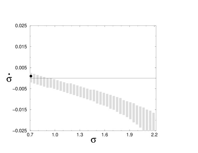
Figure 10: The shaded area indicates the region of initial conditions for which the system has a nonsingular evolution, and the dot corresponds to the value actually chosen in the solution displayed in Figs. 7-9. We have displayed only the part of the plane with $\sigma>\sigma_{\rm sd}=\log 2$, since modular invariance ensures that the figure is invariant under the transformation $\sigma\rightarrow\sigma_{\rm sd}-\sigma$.

(a)

(b)

Figure 11: (a) $\dot{\varphi}_{E}$ and (b) $H_{E}$ against string time.

4 Transition to a D-brane dominated regime

We now discuss the limitations on the validity of our solutions. As it is clear from Fig. 9, at large values of time we are deep into the strong coupling regime, $g^{2}\gg 1$. Can we still believe our solutions? In our action we have included the corrections to the Kähler potential at all perturbative orders, while other operators, like $R$ and $R_{\mu\nu\rho\sigma}^{2}$ are protected by non renormalization theorems. Therefore, despite the ambiguities that we have discussed for the four-derivative terms, due in particular to naked $R_{\mu\nu}^{2}$ and $R^{2}$ terms, one might be tempted to argue that the solution is at least representative of the behaviour at strong coupling. However, this point of view is untenable, and at some point the perturbative approach itself breaks down.

To understand this point, it is useful to work in the Einstein frame. The two-derivative part of our action then reads

$${\cal S}^{E}_{2}=\frac{1}{2\alpha^{\prime}}\int d^{4}x\sqrt{-g}\left[R-\frac{1}{2}Z_{\varphi}\partial_{\mu}\varphi\partial^{\mu}\varphi-\frac{3}{2}\partial_{\mu}\sigma\partial^{\mu}\sigma\right]$$ (39)

with

$$Z_{\varphi}=1-2e^{\varphi}G(\varphi)=1-2e^{\varphi}\left(\frac{3\kappa}{2}\right)\frac{6+\kappa e^{\varphi}}{(3+\kappa e^{\varphi})^{2}}\,.$$ (40)

At weak coupling $e^{\varphi}G(\varphi)\ll 1$ and the kinetic term of the dilaton has the ‘correct’ sign. However, as $e^{\varphi}\rightarrow\infty$, $e^{\varphi}G(\varphi)\rightarrow 3/2$ and $Z_{\varphi}<0$; $Z_{\varphi}$ vanishes at a critical value of $g^{2}=e^{\varphi}$ given by

$$g_{c}^{2}=\frac{3}{2\kappa}\left(\sqrt{6}-2\right)\simeq\frac{0.67}{\kappa}\,.$$ (41)

At $e^{\varphi}>g_{c}^{2}$ it appears that the dilaton becomes ghost-like. The situation is quite similar to what happens in Seiberg-Witten theory [41], and the physical interpretation is the same. We can rescale the dilaton so that it has a canonically normalized kinetic term $(-1/2)\partial^{\mu}\varphi\partial_{\mu}\varphi$, and in terms of the rescaled dilaton the four-derivative interactions, and in general all interactions involving the dilaton, become strong as we approach $g_{c}$, and formally diverge at the critical point. This signals that the effective action approach that we have used breaks down and we must move to a new description, where the light degrees of freedom are different. In the Seiberg-Witten model the new weakly coupled modes are related to the original ones by an S-duality transformation. In string theory the S-dual variables are given by D-branes: for instance, in the Einstein frame, a fundamental string has a tension $g^{1/2}/(2\pi\alpha^{\prime})$ while a D-string has a tension $g^{-1/2}/(2\pi\alpha^{\prime})$ [13]. This suggest that, if the cosmological evolution enters the regime $e^{\varphi}>g^{2}_{c}$, the effective action approach that we have used breaks down, and we enter a new regime, which cannot be described in terms of a classical evolution of massless modes of a closed string; in this regime we must resort to a description in terms of D-branes.

More precisely, the condition $Z_{\varphi}=0$ identifies the critical point only if $\dot{\varphi},H$ can be neglected. In fact, the equation of motion for $\varphi$ in the Einstein frame reads (we insert for future use also a potential $V(\varphi)$)

$$M_{\varphi}\ddot{\varphi}_{E}=-3AH_{E}\dot{\varphi}_{E}-V^{\prime}\,,$$ (42)

where

$$M_{\varphi}=\left[1-2e^{\varphi}G(\varphi)-3\Delta(\sigma)\dot{\varphi}_{E}^{2}\right]+\ldots\,,$$ (43)

and

$$A=1-2e^{\varphi}G(\varphi)-\Delta(\sigma)\dot{\varphi}_{E}^{2}+\ldots\,.$$ (44)

The dots denote tree-level $\alpha^{\prime}$ corrections (which are neglegible at the later stage of the evolution). We recall that we found regular solutions for $\Delta<0$. So we see that, if we include the effect of the term $|\Delta|\dot{\varphi}_{E}^{2}$, the critical line is given by the condition $M_{\varphi}=0$ or

$$Z_{\varphi}+3|\Delta|\dot{\varphi}_{E}^{2}=0\,,$$ (45)

rather than $Z_{\varphi}=0$. Of course when $\dot{\varphi}_{E}$ approaches one we should at least include all higher powers in the $\alpha^{\prime}$ expansion. More importantly, in the regime where $H$ or $\dot{\varphi}$ approach one other restrictions on the validity of the effective action appear, and have been discussed in ref. [14], embedding the 10-dimensional theory into 11-dimensional M-theory compactified on $S^{1}$. In Fig. 12 (adapted from ref. [14]) on the vertical axis we show $H$, in the string frame. This is an indicator of the curvature and therefore of the typical energy scale of the solution. One might as well use $\dot{\varphi}$, but of course precise numerical values here are not very important. In this graph we prefer to use the string frame quantity $H$ because in this case the $\alpha^{\prime}$ corrections become important when $H\sim 1$, while in terms of $H_{E}$ this condition becomes $e^{-\varphi}H_{E}^{2}\sim 1$.

The solid line $H\sim 1/g$ separates the region where an effective 10-dimensional description is possible, from the truly 11-dimensional regime. The region just above the line labelled 11d-Sugra is described by 11-dimensional supergravity, while above the line labelled Dp-branes we are in the full M-theory regime. For a discussion of the crossover between these regimes we refer the reader to ref. [14]. Of course, again, the position of the line separating the full M-theory regime from the 11-D supergravity regime is only indicative, and we have arbitrarily chosen its position so that it meets the curve $H=1/g$ exactly at $H=g=1$.

On the 10-dimensional side we have also drawn as a solid line the curve given by eq. (45), which is another critical line where a change of regime occurs. When $\dot{\varphi}_{E}$ is not small, the form of this curve is only indicative. The position of $g_{c}$ depends on $\kappa$, eq. (41), and the graph refers to a $Z_{6}$ orbifold, $\kappa\simeq 0.19$. After the curve enters in the 11-dimensional region it is not anymore meaningful. The label ‘S-duality’ means that, crossing this line, we enter a regime where the light degrees of freedom are related to the original ones by S-duality. On the same figure we display the solution of Fig. 7a, labelled by the arrows. The solution for $H$ will eventually decrease, but this only happens at very large values of $g^{2}$ (see Fig. 9), and we see that the solution enters the 11-dimensional domain before it starts decreasing. At this point, it looses its validity.

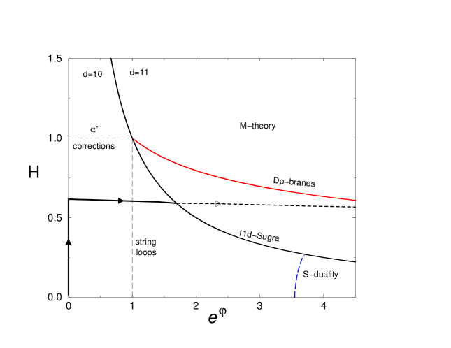
Figure 12: The ‘phase diagram’ of M-theory compactified on $S^{1}$. See the text for explanations of the various lines. The cosmological solution found in sect. 3 is marked by the arrows.

Finally, we found that it is not possible to stabilize the dilaton in our solution at a minimum of a potential, as could be generated for instance by gaugino condensation [43]. In fact at the later stage of the evolution the tree level $\alpha^{\prime}$ corrections are neglegible, as we see in Fig. 7a, and $M_{\varphi}\simeq 1-2e^{\varphi}G(\varphi)+3|\Delta|\dot{\varphi}_{E}^{2}$. If we would stabilize $\varphi$ around the minimum of the potential, it should first oscillate around the minimum and at the inversion points $\dot{\varphi}_{E}=0$, so that here the coefficient of $\ddot{\varphi}_{E}$ in eq. (42) becomes $\simeq Z_{\varphi}$. As shown in Fig. 13, this quantity is negative after we cross the $H_{E}>0$ line. As we discussed, this is not a problem for the consistency of the solution as long as $\dot{\varphi}$ is not small (in fact, Fig. 12 shows that the limitation on the validity of the solution is rather given by the crossing into the 11-dimensional region), but it is clear that no consistent solution with $\dot{\varphi}_{E}=0$ can be obtained trying to stabilize the dilaton with a potential. In fact, if we try to force $\dot{\varphi}_{E}$ to a small value, the coefficient of $\ddot{\varphi}_{E}$ in eq. (42) becomes approximately equal to $Z_{\varphi}$, which at this stage is negative. Therefore the evolution runs away from the minimum of the potential. Numerically, we have found that, including a potential in the numerical integration of the equations of motion, when the solution approaches the minimum of the potential the numerical precision, monitored by the constraint equation, degrades immediately and the solution explodes.

Therefore, in our scenario, the problem of the dilaton stabilization can only be solved after the solution enters in the non-perturbative regime.

Figure 13: The evolution of $Z_{\varphi}\equiv 1-2e^{\varphi}G(\varphi)$ close to the point where $H_{E}$ becomes positive, against string frame time.

5 Conclusions

In this paper we have tried to penetrate into the strong coupling regime of the cosmological evolution derived from string theory. This regime is crucial for an understanding of the big-bang singularity in string theory, but since loop corrections do not tame the growth of the coupling while remaining within the weak coupling domain, it is clear that a knowledge limited to, say, one-loop corrections is of little use, and we really need to have at least a glimpse into the structure of the corrections at all perturbative orders. Luckily, for the effective action of orbifold compactifications of heterotic string theory, supersymmetry and modular invariance impose strong constraints on the form of the corrections at all orders. In particular, the kinetic terms of the dilaton is known exactly, while other operators, like $R$ and $R_{\mu\nu\rho\sigma}^{2}$, are protected by non-renormalization theorems. Therefore, in spite of some ambiguities in the choice of the four-derivative terms, present both at tree level and for their loop corrections, one can try to investigate string cosmology beyond the weak coupling domain, and to obtain at least some indications of what a well motivated stringy scenario looks like.

As a first step, we have therefore tried to push this perturbative approach as far as possible, following the evolution even in the strong coupling domain $g\gg 1$. We have found solutions with interesting properties, that in the string frame start with a pre-big-bang superinflationary phase, go through a phase with $H,\dot{\varphi}$ approximately constant and of order one in string units, (a phase that replaces the big-bang singularity) and then match to a regime with $H,\dot{\varphi}$ decreasing. Apart from their intrinsic interest, these solutions provide an illustration of the interplay between $\alpha^{\prime}$ and loop corrections in string cosmology, and give an explicit realization of the general picture emerged from the works [1,5-12]. Probably the main element that is missing from this part of the analysis is the inclusion of non-local terms. These might model the backreaction due to quantum particles production, which might play an important role in the graceful exit transition [42]. Unfortunately, these are quite difficult to include in a numerical analysis.

Despite some nice properties, the cosmological model that we have presented still have some unsatisfactory features, and in particular the dilaton could not be stabilized with a potential, and so this model cannot be the end of the story.

On the other hand we have found that, if we look at our solution from the broader perspective of 11-dimensional theory, it ceases to be valid as soon as we enter into the strong coupling region, even if one includes perturbative corrections at all orders. Thus, we think that our analysis reveals quite clearly the direction that should be taken to make further progress. As already discussed in ref. [14], when we move toward large curvatures we meet critical lines in the $(H,g)$ plane, beyond which D-branes becomes the relevant degrees of freedom. Here we have found another critical line at strong coupling; beyond this line the light modes relevant for an effective action approach are obtained by an S-duality transformation and are therefore again naturally interpreted as D-branes. The combination of these critical lines, shown in fig. 12, and the behaviour of our solutions, also displayed on the same graph, suggest that the evolution enters unavoidably the regime where new descriptions set in. The understanding and the smoothing of the big-bang singularity therefore requires the use of truly non-perturbative string physics.

Acknowledgments. We thank Maurizio Gasperini, Ken Konishi, Kostas Kounnas, Toni Riotto, Gabriele Veneziano and Fabio Zwirner for useful discussions. We are grateful to Ramy Brustein for very useful comments on the manuscript.

References

- [1] G. Veneziano, Phys. Lett. B265 (1991) 287; M. Gasperini and G. Veneziano, Astropart. Phys. 1 (1993) 317; Mod. Phys. Lett. A8 (1993) 3701. An up-to-date collection of references on string cosmology can be found at http://www.to.infn.it/ gasperin/
- [2] G. Veneziano, Phys. Lett. B406 (1997) 297; M. S. Turner and E. J. Weinberg, Phys. Rev. D56 (1997) 4604; M. Maggiore and R. Sturani, Phys. Lett. B415 (1997) 335; A. Buonanno, K. A. Meissner, C. Ungarelli and G. Veneziano, Phys. Rev. D57 (1988) 2543; A. Buonanno, T. Damour and G. Veneziano, CERN-TH/98-187 (June 1998), hep-th/9806230.
- [3] M. Gasperini and G. Veneziano, Phys. Rev. D50 (1994) 2519; R. Brustein, M. Gasperini, M. Giovannini and G. Veneziano, Phys. Lett. B361 (1995) 45; M. Gasperini, M. Giovannini and G. Veneziano, Phys. Rev. Lett. 75 (1995) 3796; R. Brustein, M. Gasperini and G. Veneziano, Phys. Rev. D55 (1997) 3882; A. Buonanno, M. Maggiore and C. Ungarelli, Phys. Rev D55 (1997) 3330; B. Allen and R. Brustein, Phys. Rev. D55 (1997) 3260; M. Maggiore, Phys. Rev. D56 (1997) 1320; R. Brustein and M. Hadad, Phys. Rev. D57 (1998) 725; M. Gasperini and G. Veneziano, hep-ph/9806327, Phys. Rev. D, in press; E. J. Copeland, J. E. Lidsey and D. Wands, hep-th/9809105, Phys. Lett. B (in press).
- [4] R. Brustein and P. Steinhardt, Phys. Lett. B302 (1993) 196.
- [5] R. Brustein and G. Veneziano, Phys. Lett. B329 (1994) 429.
- [6] N. Kaloper, R. Madden and K.A. Olive, Nucl. Phys. B452 (1995) 677, Phys. Lett. B371 (1996); R. Easther, K. Maeda and D. Wands, Phys. Rev. D53 (1996) 4247.
- [7] S. Rey, Phys. Rev. Lett. 77 (1996) 1929; M. Gasperini and G. Veneziano, Phys. Lett. B387 (1996) 715.
- [8] M. Gasperini, M. Maggiore and G. Veneziano, Nucl. Phys. B494 (1997) 315.
- [9] M. Maggiore, Nucl. Phys. B525 (1998) 413.
- [10] R. Brustein and R. Madden, Phys. Lett B410 (1997) 110.
- [11] R. Brustein and R. Madden, Phys. Rev. D57 (1998) 712.
- [12] R. Brustein and R. Madden, hep-th/9901044.
-
[13]
See for example: J. Polchinski, TASI
lectures on D-branes, hep-th/9611050;
C. Bachas, Lectures on D-branes, hep-th/9806199;
W. Taylor, Lectures on D-branes, Gauge Theory and M(atrices), hep-th/9801182. - [14] M. Maggiore and A. Riotto, D-branes and Cosmology, hep-th/9811089, to appear in Nucl. Phys. B.
- [15] A. Strominger, Nucl. Phys. B451 (1995) 96; H. Ooguri and C. Vafa, Phys. Rev. Lett. 77 (1996) 3296.
- [16] M. Douglas, D. Kabat, P. Pouliot and S. Shenker, Nucl. Phys. B485 (1997) 85.
- [17] F. Larsen and F. Wilczek, Phys. Rev. D55 (1997) 4591.
- [18] T. Banks, W. Fischler and L. Motl, Dualities versus Singularities, hep-th/9811194.
- [19] J.-P. Derendinger, S. Ferrara, C. Kounnas and F. Zwirner, Nucl. Phys. B372 (1992) 145.
- [20] J.-P. Derendinger, S. Ferrara, C. Kounnas and F. Zwirner, Phys. Lett. B271 (1991) 307.
- [21] V. Kaplunovsky, Nucl. Phys. B307 (1988) 145.
- [22] L. Dixon, V. Kaplunovsky and J. Louis, Nucl. Phys. B355 (1991) 649.
- [23] V. Kaplunovsky and J. Louis, Nucl. Phys. B422 (1994) 57.
- [24] I. Antoniadis, K. Narain and T. Taylor, Phys. Lett. B267 (1991) 37.
- [25] G. Cardoso and B. Ovrut, Nucl. Phys. B369 (1992) 351; Nucl. Phys. B392 (1993) 315.
- [26] I. Antoniadis, E. Gava and K. Narain, Phys. Lett. B283 (1992) 209.
- [27] I. Antoniadis, E. Gava and K. Narain, Nucl. Phys. B383 (1992) 93.
- [28] L. Ibáñez and D. Lüst, Nucl. Phys. B382 (1992) 305.
- [29] G. Cardoso and B. Ovrut, Nucl. Phys. B418 (1994) 535.
- [30] G. Cardoso, D. Lüst and B. Ovrut, Nucl. Phys. B436 (1995) 65.
- [31] K. Förger, B. Ovrut, S. Theisen and D. Waldram, Phys. Lett. B388 (1996) 512.
- [32] M. Chemtob, Phys. Rev. D53 (1996) 3920; Systematics of string loop threshold corrections in orbifold models, hep-th/9703026.
- [33] E. Kiritsis, C. Kounnas, P. Petropoulos and J. Rizos, Nucl. Phys. B483 (1997) 141.
- [34] E. Kiritsis, C. Kounnas, P. Petropoulos and J. Rizos, On the heterotic effective action at one loop; gauge couplings and the gravitational sector, hep-th/9605011.
- [35] C. Callan, D. Friedan, E. Martinec and M. Perry, Nucl. Phys. B262 (1985) 593; E. Fradkin and A. Tseytlin, Phys. Lett. B158 (1985) 316; Nucl. Phys. B261 (1985) 1.
- [36] R. Metsaev and A. Tseytlin, Nucl. Phys. B293 (1987) 385.
- [37] S. Foffa, M. Maggiore and R. Sturani, Phys. Rev. D59:043507 (1999).
- [38] I. Antoniadis, J. Rizos and K. Tamvakis, Nucl. Phys. B415 (1994) 497.
- [39] M. Shifman and A. Vainshtein, Nucl. Phys. B277 (1986) 456; Nucl. Phys. B359 (1991) 571.
- [40] J.P. Derendinger, F. Quevedo and M. Quiròs, Nucl. Phys. B428 (1994) 282.
- [41] N. Seiberg and E. Witten, Nucl. Phys. B426 (1994) 19; ibid. B431 (1994) 484.
- [42] G. Veneziano, in Effective theories and fundamental interactions, Erice 1996, A. Zichichi ed. (World Scientific, Singapore, 1997), pag. 300; A. Buonanno, K. Meissner, C. Ungarelli and G. Veneziano, JHEP 01 (1998) 004.
- [43] G. Veneziano and S. Yankielowicz, Phys. Lett. B113 (1982) 231.