hep-th/9902170 Charged AdS Black Holes and Catastrophic Holography

Abstract

We compute the properties of a class of charged black holes in anti–de Sitter space–time, in diverse dimensions. These black holes are solutions of consistent Einstein–Maxwell truncations of gauged supergravities, which are shown to arise from the inclusion of rotation in the transverse space. We uncover rich thermodynamic phase structures for these systems, which display classic critical phenomena, including structures isomorphic to the van der Waals–Maxwell liquid–gas system. In that case, the phases are controlled by the universal “cusp” and “swallowtail” shapes familiar from catastrophe theory. All of the thermodynamics is consistent with field theory interpretations via holography, where the dual field theories can sometimes be found on the world volumes of coincident rotating branes.

I Introduction

There is evidence that there is a correspondence[1, 2, 3] between gravitational physics in anti–de Sitter space–time and particular types of conformal field theory in one dimension fewer. This duality is a form of “holography” [5] and a part of the correspondence operates by identifying the field theory as living on the boundary of anti–de Sitter (AdS) space–time.

To be more precise, AdS_n+1$\times{\cal M}^{m}$ is the space–time of interest, and there is some $(n{+}m{+}1)$–dimensional theory of gravity compactified on it. The manifold ${\cal M}^{m}$ can be an $m$–sphere, $S^{m}$. The corresponding field theory is an $n$–dimensional conformal field theory living on a space with the topology of the boundary of AdS_n+1. The isometries of the manifold ${\cal M}^{m}$ appear as global symmetries of the field theory: R–symmetries if the theory is supersymmetric.

This particular form of duality between gravity and field theory is certainly intriguing. The large $N$ limit (where $N$ is the rank of the $SU(N)$ gauge group for the four dimensional Yang–Mills field theory, with appropriate generalizations for other dimensions) of the field theory —at strong ’t Hooft coupling— corresponds to classical supergravity. As pointed out in ref. [7], following the observations in ref. [3], the old program of semi–classical quantum gravity finds a new lease on life in this setting, as computations such as those performed with gravitational instantons (at least in AdS) should have natural field theory interpretations.

In this paper, we study the thermal properties of Einstein–Maxwell AdS (EMadS) charged black holes, and find behaviour consistent with field theory interpretations. We do this for arbitrary dimensions (greater than 3— see section VII for comments on $D{=}3$) and determine the thermal phase structure of the corresponding field theories. The cases of AdS₄, AdS₅ and AdS₇ are particularly interesting of course, as they correspond to the theories found on the world volumes of M2–, D3–, and M5–branes, respectively. The D3–brane case is $D{=}4$, ${\cal N}{=}4$ supersymmetric $SU(N)$ Yang–Mills theory, while the others are exotic superconformal field theories [26]. We remark on the field theory interpretation of our new results in the light of holography.

This paper is also of relevance beyond mere considerations of holography. Some of the black hole solutions and their properties (thermodynamic or otherwise) are presented here for the first time. In particular, the Lagrangian action calculations and subsequent determination of the phase structure are presented in their entirety here.

In section II, we present an ansatz for obtaining the Einstein–Maxwell truncation of gauged AdS supergravity with appropriate compactifications of $D{=}11$ supergravity on $S^{7}$, and $D{=}10$ type IIB supergravity on $S^{5}$. In the planar or infinite–volume limit, the charged black holes in Einstein–Maxwell–Anti–deSitter correspond to the near horizon limits of rotating M2– and D3–branes. In section III, we display the solutions and note some of their properties. The computation of the action of the solutions using a Euclidean section is performed in section IV, and their thermodynamic properties are uncovered in section V.

As the Einstein–Maxwell–Anti–deSitter truncation is naturally associated to rotating branes, (at least in the case of EM–AdS₄ and EM–AdS₅, see section II) it is very natural to suppose that there is an associated dual field theory, arising on the world-volume of some branes. These would be the familiar conformal field theories —the $D{=}4$, ${\cal N}{=}4$ Yang–Mills theory (for coincident D3–branes) and the conformal field theory on the world–volume of coincident M2–branes. The case of EM–AdS₇ (i.e., without additional scalars) is not related to a rotating–brane truncation of the AdS${}_{7}{\times}S^{4}$ gauged supergravity (because $S^{4}$ is even dimensional) and so we cannot declare that the dual field theory is the theory on the world–volume of a rotating M5–brane. However, we regard AdS holography as a phenomenon which exists independently of string– and M–theory contexts[3, 7]. Hence, in other dimensions beyond $D{=}4$ and 5, we expect that there is a dual theory. In particular, for EM–AdS₇ the dual field theory is probably a close cousin of the M5–brane theory.

The dual field theories have their supersymmetry (if they had any to start with) broken due to coupling to a global background $U(1)$ current (as well as turning on a non–zero temperature). The CFT is in a thermal ensemble for which a certain $U(1)$ charge density has also been “turned on”. In the ensemble, the expectation value of this charge breaks the global $SO(m{+}1)$ R–symmetry of the CFT. On the AdS side, the electromagnetic charge carried by the black holes is in the same $U(1)$ of corresponding $SO(m{+}1)$ gauge group.

We find very interesting phase structures at intermediate temperatures (in finite field theory volume), as a result of studying two complementary thermodynamic ensembles: We study thermodynamic ensembles with fixed background potential —in which case the background is AdS with a constant fixed potential— and we also study a fixed localized charge ensemble, for which the background is an extremal black hole with that charge.

In all cases, at sufficiently high temperature the physics is dominated by highly non–extreme black holes, and we therefore recover the “unconfined” behaviour characteristic of the associated field theories[3, 4]. The finite horizon size of the black holes controls the behaviour of the expectation value of spatial Wilson lines accordingly, yielding the area law behaviour, as follows from ref.[4].

At intermediate temperatures, in the fixed charge ensemble, the presence of charge allows a new branch of black hole solutions to modify the qualitative phase structure in the low charge regime, resulting in a very interesting phase structure about which we will have more to say later in this section.

Intriguingly, as there is an extremal —but non–supersymmetric— black hole with non–zero entropy even at zero temperature, we must conclude something interesting about the field theory in the presence of the global background $U(1)$ current: There must still be at $T{=}0$ a large number of states (with the given charge) available to the field theory in order to generate this entropy. For the case where we hold the potential (i.e., not the charge) fixed, we do not expect that this is the ground state, because the extremal black hole can decay into Kaluza–Klein particles, leaving AdS. This is because the extremal black hole is not supersymmetric.

This subtlety does not arise in the standard Gibbons–Hawking calculus of the thermodynamics of black holes —which we use here— because the calculations are not sensitive to the ability of the black holes to emit charged particles.

That the extremal black hole can decay by emitting charged Kaluza–Klein particles here follows from the fact that the charge descends from rotation in higher dimensions. There are well–known classical processes for reducing the rotation of objects like black holes by scattering[8], and therefore in the context of quantum field theory, one has the analogous processes of emission in superradiant modes[9]. The same superradiant emission was considered in the context of charged black holes in ref.[10, 11]. Thus one should expect the extremal black hole in the EMadS truncation to decay via such supperradiant emission. Of course, the usual thermal Hawking radiation may also tend to discharge nonextremal black holes[11, 12, 13]. In the fixed potential ensemble, as the charge of the black hole is allowed to fluctuate while it is in contact with the thermal reservoir, superradiant and Hawking emission processes can occur to reduce the charge of the black hole, allowing it to decay back to AdS (plus charge). However, in the fixed charge thermodynamic ensemble (with varying potential), the extremal black hole is expected to be the long–lived state at zero temperature.

Translating the formula for the entropy to the field theory we find, for example, that the four dimensional Yang–Mills theory (in the presence of the global background $U(1)$ current) has a zero–temperature entropy which goes like $S{\sim}{\bar{Q}}$ for large black holes, where $\bar{Q}$ measures the total charge in units of the minimal charge of Kaluza–Klein excitations (i.e., $1/l$), and is proportional to the volume, $V_{3}$, of the field theory. Notice that the result for the four dimensional field theory is consistent with confinement at $T{=}0$, as the result is independent of $N$. Confinement also follows from the fact that at $T{=}0$, the Euclidean section of the solution has no bolt, and therefore temporal Wilson lines will always be homotopic to zero, and therefore have zero expectation value. Meanwhile, spatial Wilson lines cannot interact with the horizon to produce an area law dependence, because at extremality the horizon recedes infinitely far away down a Bertotti–Robinson throat.

The phase structure which we obtain in each thermodynamic ensemble is summarized in figure 1.

FIG. 1.: A summary of the phase structure of the fixed potential (left) and fixed charge (right) thermodynamic ensembles. The $T{=}0$ line gives extremal black holes, although only in the fixed charge case do they not decay into AdS. The $Q{=}0$ line is the Hawking–Page system of uncharged black holes. (Other labeling is explained in sections V and VI.)

The astute reader will recognize the figure on the right as the classic phase diagram of the liquid–gas system! To translate, our $Q$ is like the temperature $T$ of the fluid while $1/T$ is like the pressure $P$. The non–extreme black holes of type (1) (“small”) and (3) (“large”) (see section IV and V for explanation) are like the liquid phase and the gaseous phase, respectively. The critical line (“vapour pressure curve”) represents the place at which a first order phase transition between the liquid and gas occurs. As is well known, there is a critical temperature at which the vapour pressure curve terminates, representing the fact that above a critical temperature, one can convert a liquid to a gas continuously. This translates here into a critical charge above which the two types of black hole can be continuously converted into one another with no discontinuity in their size.

That this system (first modeled by van der Waals[14], with a crucial modification by Maxwell) appears in this AdS black hole thermodynamics is fascinating, and would not have been possible (at least in this way) without the presence of the extra branches of solutions which appear when there is negative cosmological constant. We discuss this further in sections V and IV. Further fascination may be found in the fact that the explicit shape of the free energy surface (as a function of $Q$ and $T$) is that of the classic “swallowtail” catastrophe, familiar from the study of bifurcations[34]. The control surface of the “cusp” catastrophe also appears, which (of course) follows from the well known fact that it is the shape of the van der Waals equation of state, viewed as a surface in $P,V,T$ space.

That these shapes appear in this context suggests that there is some exciting universality to be explored here: Catastrophe theory is largely a classification of the possible distinct types of bifurcation shapes that can occur in a wide variety of complex systems. This classification (which, for the common “elementary” cases is of A–D–E type) is equivalent to the (perhaps more familiar) classfication of singularities[35]. It is of considerable interest to discover just what circumstances might give rise to the other members of the classification. Recalling that this all translates via holography into properties of a dual field theory, we would learn a great deal about universal phase structures which can occur there also.

II Einstein–Maxwell–AdS from spinning branes

Physics near the horizon of supergravity branes can be described in terms of spontaneous compactification of supergravity. In the case of non–dilatonic branes —which will be the focus of the paper— when the compactification takes place on a round $m$–sphere the low energy degrees of freedom are described by an effective theory of Einstein gravity with a negative cosmological constant coupled to $SO(m{+}1)$ gauge fields. The Schwarzschild–Anti–deSitter black hole solutions of this theory have been used in the context of the AdS/CFT correspondence to infer thermal properties of the dual field theories [3, 4].

A natural extension of this program is to study AdS black holes which are charged under a subgroup of the gauge symmetry of the gauged supergravity. Solutions of Einstein–Maxwell–anti–deSitter in some dimensions are known, but in the context of string/M–theory, it is also interesting to determine how to make a truncation of the type IIB supergravity, or of 11 dimensional supergravity, which gives the EMadS effective action. In other words, we must make certain higher–dimensional choices which will result in the removal of the generic coupling of the $F^{2}$ term to scalars resulting from the Kaluza–Klein reduction.

Amusingly, one simple way to introduce (gauge) charge on the black holes is by simply spinning —or twisting— the transverse (angular) sphere that becomes the compact space. Decoupling of the scalars is accomplished by choosing the spins in a maximally symmetric way. To be concrete, take ten dimensional IIB supergravity, with the metric ansatz

$$ds^{2}_{10}=g^{5}_{\mu\nu}dx^{\mu}dx^{\nu}+l^{2}\sum_{i=1}^{3}[d\mu_{i}^{2}+\mu_{i}^{2}(d\varphi_{i}+\frac{2}{\sqrt{3}}A_{\mu}dx^{\mu})^{2}],$$ (1)

where $g^{5}_{\mu\nu}$ is a five-dimensional metric, $\mu,\nu=0\dots 4$, the variables $\mu_{i}$ are direction cosines on $S^{5}$ (and therefore are not independent, $\sum_{i=1}^{3}\mu_{i}^{2}=1$ —we follow the notation of[17]), and the $\varphi_{i}$ are rotation angles on $S^{5}$. The ansatz for the RR 5-form field strength has “electric” components

$$F^{(5)}_{e}=-{4\over l}\varepsilon^{(5)}+{l^{3}\over\sqrt{3}}\sum_{i=1}^{3}d\mu_{i}^{2}d\phi_{i}\,*^{5}\!dA,$$ (2)

while the dual “magnetic” components are given by $F^{(5)}_{m}{=}*\!F^{(5)}_{e}$. In eqn. (2), $\varepsilon^{(5)}$ is the volume form on the reduced five-dimensional space, and $*^{5}$ denotes Hodge duality on this space.

The parameter $l$ measures the size of the $S^{5}$ and is given by the flux of the 5–form field across the $S^{5}$. Notice that a component $A_{t}$ in the time direction is interpreted as rotation of the $S^{5}$ in its three independent rotation planes, in equal amounts. Components in the spatial direction would instead be ‘twists.’ For the sake of brevity, and since in this paper we will be mainly considering $A_{t}$ components, we will refer collectively to them as “rotations”.

With this ansatz (1), the effective action in the five non–compact dimensions becomes

$$I=-{1\over 16\pi G_{5}}\int d^{5}x\sqrt{-g^{5}}\left[R+{12\over l^{2}}-{l^{2}}F^{2}-{l^{3}\over 6\sqrt{3}}\epsilon^{\mu\alpha\beta\gamma\delta}A_{\mu}F_{\alpha\beta}F_{\gamma\delta}\right].$$ (3)

This is precisely the Einstein–Maxwell–Anti–deSitter (EMadS) effective action we seek, with a Chern–Simons term. The latter is indeed required by supersymmetry in ${\cal N}{=}2$ five dimensional gauged supergravity [18], whose bosonic sector is precisely described by the action above. Note that the gauge coupling is proportional to $\sqrt{G_{5}}/l$.

The AdS${}_{5}{\times}S^{5}$ gauged supergravity theory in five dimensions has an $SO(6)$ gauge symmetry, associated with the group of isometries of $S^{5}$. This is the R–symmetry group of the dual four dimensional ${\cal N}{=}4$ superconformal Yang–Mills field theory living on the D3–branes from which this near–horizon geometry arose. The above spinning compactification corresponds to introducing rotation in the diagonal $U(1)$ of the maximal Abelian subgroup $U(1)^{3}$. Correspondingly, there must be a dual field theory to the EMadS truncation, which is simply the field theory on the world–volume of the rotating brane. From the field theory point of view, the rotation corresponds to considering states or ensembles in which the dual global $U(1)$ current (a subgroup of the $SO(6)$ R–symmetry group) has a nonvanishing expectation value. Studying EMadS gravity and its solutions will therefore be equivalent to studying properties of the conformal field theory in the presence of this background current.

A similar construction can be obtained by starting from eleven dimensional supergravity. The compactification in this case is equivalent to focusing on the near horizon region of M2–branes. In this case, take

$$ds^{2}_{11}=g^{4}_{\mu\nu}dx^{\mu}dx^{\nu}+4l^{2}\sum_{i=1}^{4}[d\mu_{i}^{2}+\mu_{i}^{2}(d\varphi_{i}+A_{\mu}dx^{\mu})^{2}],$$ (4)

leading to the AdS₄ theory with a Maxwell term

$$I=-{1\over 16\pi G_{4}}\int d^{4}x\sqrt{-g^{4}}\left[R+{6\over l^{2}}-4l^{2}F^{2}\right].$$ (5)

The reduction ansatz for the 4-form field strength is

$$F^{(4)}={3\over l}\varepsilon^{(4)}+4l^{2}\sum_{i=1}^{4}d\mu_{i}^{2}d\phi_{i}\,*^{4}\!dA,$$ (6)

where $\varepsilon^{(4)}$ is the volume form on the reduced four–dimensional space, and $*^{4}$ denotes Hodge duality on this space.

Chern–Simons terms are absent in four dimensions. Appropriate inclusion of fermions leads to four dimensional ${\cal N}{=}2$ gauged supergravity. The more general $U(1)^{4}$ theory with four independent gauge fields (i.e., four different rotation parameters) 3 scalars and ${\cal N}{=}8$ supersymmetry, as well as its black hole solutions, have been recently studied in ref. [27].

We note here that there is no analogous construction for the AdS${}_{7}{\times}S^{4}$ gauged supergravity theory. This is because $S^{4}$ is even dimensional and therefore we cannot have a symmetric split between $U(1)$ rotations, as $SO(5)$ does not have an even torus for its Cartan subalgebra. This means that we cannot relate the physics of the black hole solutions (which we write later) of the EM–AdS₇ system to the physics of rotating M5–branes of eleven dimensional supergravity. Nevertheless, as AdS holography is a phenomenon which is expected to exist independently of string or M–theory realizations, we expect that the physics does have a holographic interpretation in terms of a field theory closely related to that which resides on M5–brane world–volumes.

III Charged black holes in Anti–de Sitter space–time

The black hole solutions of the above supergravity theories in $D{=}4,5$ were originally studied in the past in refs. [18] and [19]—more recent investigations appear in refs. [21, 27]. As we have seen in the previous section, such theories can be regarded as compactifications of the type IIB and $D{=}11$ supergravities, where the gauge symmetry groups of the gauged supergravities are broken by a specific choice of rotation planes in the transverse compact spheres. Given these considerations, it is natural to study the Reissner–Nordstrom–anti–deSitter (RNadS) black holes within the context of the AdS/CFT correspondence.

Even if the bosonic Einstein–Maxwell–Anti–deSitter (EMadS) theories admit supersymmetric extensions only in certain dimensions, it is easy and convenient to perform the analysis of their black hole solutions for arbitrary dimension. For space–time dimension $n{+}1$, the action can be written as

$$I=-\frac{1}{16{\pi}G}\int_{M}d^{n+1}x\sqrt{-g}\left[R-F^{2}+\frac{n(n-1)}{l^{2}}\right],$$ (7)

with ${\Lambda}{=}{-}\frac{n(n-1)}{2l^{2}}$ the cosmological constant associated with the characteristic length scale $l$. Then the metric on RNadS may be written in static coordinates as

$$ds^{2}=-V(r)dt^{2}+\frac{dr^{2}}{V(r)}+r^{2}d{\Omega}^{2}_{n-1},$$ (8)

where $d{\Omega}^{2}_{n-1}$ is the metric on the round unit $(n{-}1)$–sphere, and the function $V(r)$ takes the form

$$V(r)=1-\frac{m}{r^{n-2}}+\frac{q^{2}}{r^{2n-4}}+\frac{r^{2}}{l^{2}}.$$ (9)

Here, $m$ is related to the ADM mass of the hole, $M$ (appropriately generalized to geometries asymptotic to AdS[20]), as

$$M={(n-1)\omega_{n-1}\over 16\pi G}m,$$ (10)

where $\omega_{n-1}$ is the volume of the unit $(n{-}1)$–sphere. The parameter $q$ yields the charge

$$Q=\sqrt{2(n-1)(n-2)}\left({\omega_{n-1}\over 8\pi G}\right)q,$$ (11)

of the (pure electric) gauge potential, which is

$$A=\left(-{1\over c}{q\over r^{n-2}}+\Phi\right)dt,$$ (12)

where

$$c=\sqrt{2(n-2)\over n-1},$$ (13)

and $\Phi$ is a constant (to be fixed below). If $r_{+}$ is the largest real positive root of $V(r)$, then in order for this RNadS metric to describe a charged black hole with a non–singular horizon at $r{=}r_{+}$, the latter must satisfy

$$\left({n\over n-2}\right)r_{+}^{2n-2}+l^{2}r_{+}^{2n-4}\geq q^{2}l^{2}.$$ (14)

Finally, we choose

$$\Phi={1\over c}{q\over r_{+}^{n-2}},$$ (15)

which then fixes $A_{t}(r_{+}){=}0$. The physical significance of the quantity $\Phi$, which plays an important role later, is that it is the electrostatic potential difference between the horizon and infinity.

If the inequality in eqn. (14) is saturated the horizon is degenerate and we get an extremal black hole. This inequality imposes a bound on the black hole mass parameter of the form $m{\geq}m_{e}(q,l)$. In the cases where the theory admits a supersymmetric embedding one could naively expect to approach a supersymmetric state as we saturate this mass bound. However, the bound that results from the supersymmetry algebra is instead [18, 19]: $m{\geq}2q$, with the $m{=}2q$ solution being a BPS state. Now, it is easy to see that the mass of the extremal black hole, $m_{e}$ is, for finite $l$, always strictly larger than $2q$ and therefore the extremal solution is non–supersymmetric. On the other hand, for the supersymmetric solution one has

$$V(r)=\left(1-{q\over r^{n-2}}\right)^{2}+{r^{2}\over l^{2}},$$ (16)

which is strictly positive everywhere and therefore one finds a naked curvature singularity at $r{=}0$. In fact, all the solutions violating the bound (14) are nakedly singular.

In the context of the AdS/CFT correspondence it is interesting to consider the limit where the boundary of AdS_n+1 is ${\hbox{{\rm I}\kern-1.99997pt\hbox{\rm R}}}^{n}$ instead of ${\hbox{{\rm I}\kern-1.99997pt\hbox{\rm R}}}{\times}S^{n-1}$ as was the case above. This can be regarded as an “infinite volume limit”, with particular relevance to the discussion of the dual field theory. It should be noted that the existence of black hole solutions in this limit is possible only due to the presence of a negative cosmological constant. In fact, black holes (and other bolts) in AdS spaces with varied topologies (even other than spherical and toroidal) have been extensively studied in recent years [24], including in the M–theory [25]. Here we will only focus on the planar (toroidal) solutions, which we will obtain by scaling the “finite volume” solutions above, as done in [4]. To this effect, introduce a dimensionless parameter $\lambda$ (which we will shortly take to infinity) and set

$$r \rightarrow\lambda^{1/n}r,\qquad t\rightarrow\lambda^{-1/n}t,$$ (17)

$$m \rightarrow\lambda m,\qquad q\rightarrow\lambda^{(n-1)/n}q,$$ (18)

while at the same time blowing up the $S^{n-1}$ as $l^{2}d\Omega_{n-1}^{2}\rightarrow\lambda^{-2/n}\sum_{i=1}^{n-1}dx_{i}^{2}$. One finds, after taking $\lambda{\to}\infty$,

$$ds^{2}=-U(r)dt^{2}+{dr^{2}\over U(r)}+{r^{2}\over l^{2}}\sum_{i=1}^{n-1}dx_{i}^{2},$$ (19)

with

$$U(r)={r^{2}\over l^{2}}-{m\over r^{n-2}}+{q^{2}\over r^{2n-4}}.$$ (20)

For the supersymmetric solution, the scaling is as above except for the scaling of $m$. To preserve supersymmetry, one must fix $m{=}2q$ and so $m{\rightarrow}m\lambda^{(n-1)/n}$ yielding

$$U(r)={r^{2}\over l^{2}}+{q^{2}\over r^{2n-4}}.$$ (21)

Notice that, compared with eqn. (20), the parameter $m$ is zero in this limit.

The resulting solution can be seen to be supersymmetric as well (i.e., the Killing spinors remain finite in the limit $\lambda{\rightarrow}\infty$, after appropriate rescaling), and nakedly singular. In this “infinite volume” limit, the solutions asymptote to AdS space with the horospheric slicing.

These planar solutions can be constructed with the appropriate decoupling limit[1] of spinning D3– or M2–branes, as mentioned previously. We refer the reader to ref.[22] for the details.

IV Action Calculation

The study of the Euclidean section ($t{\to}i\tau$) of the solution, identifying the period, $\beta$, of the imaginary time with inverse temperature, will define for us the grand canonical thermodynamic ensemble (for fixed electric potential) or the canonical ensemble (for fixed electric charge). We interpret this in terms of immersing the system into a thermal bath of quanta at temperature $T{=}1/\beta$. For pure AdS, the background consists of both charged and uncharged quanta free to fluctuate in the presence of fixed potential $\Phi$. Later, we consider the fixed $Q$ ensemble. In that case we localize all of the charge at a specific region and keep it fixed. For such a background, as AdS with a localized charge is not a solution of the EMadS equations, we use the extremal black hole solution as the background, and retain only neutral quanta in the thermal reservoir, in order to keep the charged fixed. This makes sense, even though the extreme limit has zero temperature, since the Euclidean section has no bolt and so can be assigned an arbitrary periodicity[28]. Hence, the metrics and gauge fields can be matched in the asymptotic region.

With all of this in mind we now turn to the action calculations.

A Fixed Potential

With our conventions the full Euclidean action is given by analytically continuing eqn. (7), where, as usual when the space is asymptotically AdS the Gibbons–Hawking boundary term gives a vanishing contribution. The boundary terms from the gauge field will vanish if we keep the potential $A_{t}$ fixed at infinity. Any possible Chern–Simons term will not contribute when we restrict ourselves to purely electric solutions. Imposing the equations of motion we can eliminate the factors of $R$ in order to obtain the on–shell action

$$I=\frac{1}{16{\pi}G}\int_{M}d^{n+1}x\sqrt{g}\left[\frac{2F^{2}}{n-1}+\frac{2n}{l^{2}}\right].$$ (22)

We obtain for the action (subtracting the AdS background while remembering to match the geometries of the background and black hole in the asymptotic region):

$$I=\frac{\omega_{n-1}}{16\pi Gl^{2}}\beta\left(l^{2}r_{+}^{n-2}-r_{+}^{n}-\frac{q^{2}l^{2}}{r_{+}^{n-2}}\right)=\frac{\omega_{n-1}}{16\pi Gl^{2}}\beta\left(l^{2}r_{+}^{n-2}(1-c^{2}\Phi^{2})-r_{+}^{n}\right).$$ (23)

Here, $\beta$ denotes the period of the Euclidean section of the black hole space–time. Using the usual formula for the period, $\beta{=}{4\pi}/{V^{\prime}(r_{+})}$, a little algebra yields the explicit form

$$\beta=\frac{4{\pi}l^{2}r_{+}^{2n-3}}{nr_{+}^{2n-2}+(n-2)l^{2}r_{+}^{2n-4}-(n-2)q^{2}l^{2}}.$$ (24)

This may be rewritten in terms of the potential as:

$$\beta=\frac{4{\pi}l^{2}r_{+}}{(n-2)l^{2}(1-c^{2}\Phi^{2})+nr_{+}^{2}}.$$ (25)

Note that the temperature is zero when the black hole is extremal. This is because the horizon is degenerate there, and $\beta$ diverges, together with the fact that one can smoothly approach the extremal limit from non–zero temperature. From the form of the equation for $\beta$, it is apparent that there are qualitatively two distinct types of behaviour, determined by whether $\Phi$ is less than or greater than the critical value $1/c$. In particular, for $\Phi{\geq}1/c$, $\beta$ diverges ($T$ vanishes) at $r_{+}^{2}{=}l^{2}(n-2)(c^{2}\Phi^{2}{-}1)/n$, while for $\Phi{<}1/c$, $\beta$ goes smoothly towards zero as $r_{+}{\rightarrow}0$. It is instructive to plot the temperature as a function of horizon radius (size of black hole) for these two regimes (see fig. 2).

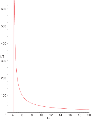
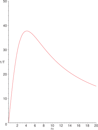
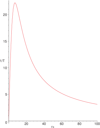
FIG. 2.: The inverse temperature vs. horizon radii, $r_{+}$, at fixed potential for $\Phi{\geq}1/c$, $\Phi{<}1/c$, and $\Phi{=}0$ respectively. (The values $n{=}4$, $G{=}1$, $l{=}10$ and $\Phi=1,0.7,0$ have been used here.) The divergence in the first graph (here, shown with a vertical line at $r_{e}{=}4.08$) is at zero temperature, where the black hole is extremal. This divergence goes away for $\Phi{<}1/c$, in general, and the curve is similar to that of the uncharged situation with zero potential, shown last.

As can be seen from the figure, the regime of large potential (i.e., $\Phi\geq 1/c$) has a unique black hole radius associated with each temperature. We will see later that this branch dominates the thermodynamics for all temperatures. Meanwhile the small potential regime has two branches of allowed black hole solutions, a branch with larger radii and one with smaller. This is qualitatively similar to the familiar case of the uncharged Schwarzschild black holes analyzed in ref. [6], (or the structure of the Taub–bolts discovered in the thermodynamic studies of ref. [7, 30]), which is the $\Phi{=}0$ limit of the situation here. Correspondingly, the smaller branch of holes is unstable, having negative specific heat. They do not play any role in the physics. (Generally, the sign of the specific heat for a black hole of radius $r_{+}$ can be inferred from the local slope of the $\beta(r_{+})$ curve. See also the discussion in section VI.)

B Fixed Charge

If we wish to consider a situation where instead of the potential at infinity, we fix the charge of the black hole, then the action (23) is not appropriate. Upon variation of the gauge field in the latter action, a boundary term results that vanishes only if we keep $A_{t}(\infty){=}\Phi$ fixed. That is, the on–shell action of the previous subsection is $I[\beta,\Phi]$. If, instead, we want to keep the charge fixed, then we must add a boundary term to $I$ [29],

$$\tilde{I}=I-{1\over 4\pi G}\int d^{n}x\sqrt{h}F^{\mu\nu}n_{\mu}A_{\nu},$$ (26)

where $n_{\mu}$ is a radial unit vector pointing outwards (notice that this boundary term is determined by the terms coming from the variation of the off–shell action (7), and not (22), which is on–gravity–shell. This distinction is only relevant for $n{>}3$). Then we get a thermodynamic function $\tilde{I}[\beta,Q]$, in terms of the variables we wish to control.

To compute the action for the fixed charge ensemble, using as background the extremal black hole, we evaluate eqn. (22) for a black hole of mass $m{>}m_{e}$ (and radius $r_{+}$), and then subtract the contribution from the extremal background. Remembering to match the geometries of the background and black hole in the asymptotic region, a straightforward calculation yields the final result

$$\tilde{I}={\omega_{n-1}\beta\over 16\pi Gl^{2}}\left[l^{2}r_{+}^{n-2}-r_{+}^{n}+{(2n-3)q^{2}l^{2}\over r_{+}^{n-2}}-{2(n-1)\over n}l^{2}r_{e}^{n-2}-{2(n-1)^{2}\over n}{q^{2}l^{2}\over r_{e}^{n-2}}\right].$$ (27)

The inverse temperature, $\beta$, is given by eqn. (24). It is useful to plot the temperature as a function of horizon radius (size of black hole) for future use. There are two basic scales in this expression for $\tilde{I}$, set by $q$ and $l$, and so we expect that there will be two distinct regimes which may display distinct phase structure: $q{\geq}q_{\rm crit}$ and $q{<}q_{\rm crit}$. For comparison, we also show the case of $q{=}0$ (see fig. 3).

The critical charge $q_{\rm crit}$ is the value of $q$ at which the turning points of $\beta(r_{+})$ appear or disappear. With $q{=}q_{\rm crit}$, the periodicity $\beta{=}\beta(r_{+},q,l)$ will have a point of inflection with respect to $r_{+}$ derivatives. Hence we can simultaneously satisfy

$${\partial\beta\over\partial r_{+}}=0={\partial^{2}\beta\over\partial r_{+}^{2}},$$ (28)

with $r_{+}{=}r_{\rm crit}$ and $q{=}q_{\rm crit}$. A little algebra then yields

$$r_{\rm crit}^{2}={(n-2)^{2}\over n(n-1)}\,l^{2}\quad{\rm and}\qquad q_{\rm crit}^{2}={1\over(n-1)(2n-3)}\left({(n-2)^{2}\over n(n-1)}\right)^{n-2}l^{2n-4}.$$ (29)

Therefore we have for $n{=}3$, $q_{\rm crit}{=}l/6$ and for $n{=}4$, $q_{\rm crit}{=}l^{2}/3\sqrt{15}.$

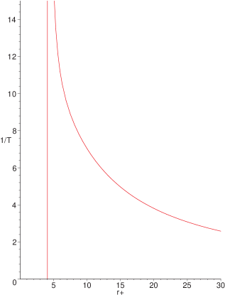
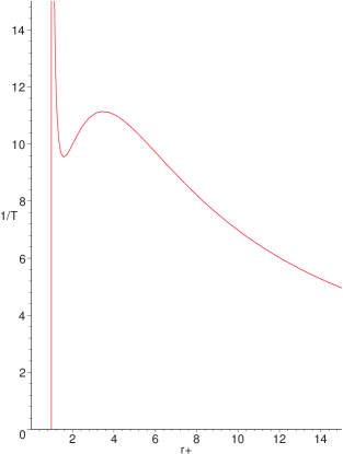
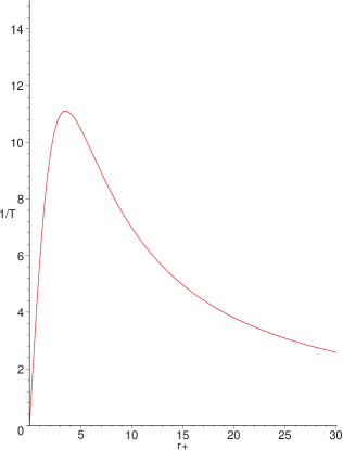
FIG. 3.: The inverse temperature vs. horizon radii, for $q{>}q_{\rm crit}$, $q{<}q_{\rm crit}$, and $q{=}0$, respectively. $q_{\rm crit}$ is the value of $q$ at which the turning points of $\beta(r_{+})$ appear or disappear. (The values $n{=}4$, $l{=}5$ and $q=25,5,0$ have been used here.) The divergences (here, shown by the vertical lines at $r_{e}{=}0.98$ and $4.05$) are at zero temperature, where the black hole is extremal. The final graph, for the uncharged case, may be thought of as a limit of the previous graphs where the divergence disappears, showing that small Schwarzschild black holes have high temperature.

In this case, the figures show that for small charge (i.e., below $q_{\rm crit}$), there can be three branches of black hole solutions, to which we will refer later. The middle branch is unstable while the branch with the smallest radii is new, and will play an interesting role in the thermodynamics. For zero charge, we return to the familiar two branch situation of Schwarzschild, while for large charge, we have a situation analogous to that seen for the large fixed potential.

V Thermodynamics and phase structure

A Fixed Potential

This is the grand canonical ensemble, at fixed temperature and fixed potential. The grand canonical (Gibbs) potential is $W{=}I/\beta{=}E{-}TS{-}\Phi Q.$ Using the expression in eqn. (23), we may compute the state variables of the system as follows:

$$E= \left(\frac{\partial I}{\partial\beta}\right)_{\Phi}-\frac{\Phi}{\beta}\left(\frac{\partial I}{\partial\Phi}\right)_{\beta}=\frac{(n-1)\omega_{n-1}}{16\pi G}m=M,$$ (30)

$$S= \beta\left(\frac{\partial I}{\partial\beta}\right)_{\Phi}-I=\frac{\omega_{n-1}r_{+}^{n-1}}{4G}=\frac{A_{H}}{4G},\qquad{\rm and}$$ (31)

$$Q= -\frac{1}{\beta}\left(\frac{\partial I}{\partial\Phi}\right)_{\beta}=\sqrt{2(n-2)(n-1)}\left(\frac{\omega_{n-1}}{8\pi G}\right)q.$$ (32)

Together, they indeed satisfy the first law: $dE=TdS+\Phi dQ$.

In order to study the phase structure and stability, we must observe the free energy $W{=}I/\beta$ as a function of the temperature. It is shown in figure 4.

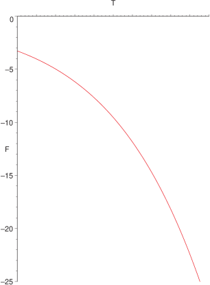
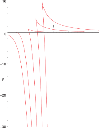
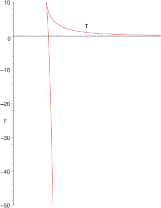
FIG. 4.: On the left is a graph of the free energy vs. temperature for fixed potential ensemble for large $\Phi$. (The values $n{=}4$, $G{=}1$, $l{=}10$, $\Phi{=}1$ have been used here.) The center graph depicts a family of free energy curves for different values of $\Phi$. Note the crossover from the cusp ($\Phi{<}1/c$) to the single branch ($\Phi{>}1/c$) behaviour. On the right is the free energy curve for the uncharged (or $\Phi{=}0$) ensemble, showing the physics familiar from the Schwarzschild case: visible are the two branches consisting of smaller (unstable) and large (stable) black holes. The entire unstable branch has positive free energy while the stable branch’s free energy goes (rapidly, on this scale) negative for all $T{>}T_{c}$.

The interpretation of this is as follows. At any non–zero temperature, for large potential ($\Phi{>}1/c$) the charged black hole is thermodynamically preferred, as its free energy (relative to the background of AdS with a fixed potential) is strictly negative for all temperatures.

This behaviour differs sharply from the small potential ($\Phi{<}1/c$) situation, which is qualitatively the same as the uncharged case: In that situation, in finite volume, the free energy is positive for some range $0{<}T{<}T_{c}$, and it is only above $T_{c}$ that the thermodynamics is dominated by Schwarzschild black holes (the larger, stable branch), after their free energy is negative. (See the center graphs in figure 4.)

So for high enough temperature in all cases the physics is dominated by non–extremal black holes. In this case, (after converting gravitational to field theory quantities) the free energy and entropy behave at ultra–high temperature as

$$F \sim V_{n-1}T^{n}N^{p(n)}$$ (33)

$$S \sim V_{n-1}T^{n-1}N^{p(n)},$$ (34)

where $V_{n-1}$ is the $(n{-}1)$–dimensional spatial volume upon which the field theory lives. This is the “unconfined” behaviour appropriate to the dual $n$–dimensional field theory. The function $p(n)$ is $2$ when $n{=}4$; $3/2$ when $n{=}3$; $2/3$ when $n{=}6$. The resulting power of $N$ shows how the number of unconfined degrees of freedom of the theory goes with $N$, by analogy with the case of $n{=}4$ where $N^{2}$ counts the dependence on the number of degrees of freedom on $N$ for an $SU(N)$ gauge theory.

At low temperatures, and for $\Phi{>}1/c$, we have something very new. Notice that as we go to $T{=}0$, the free energy curve approaches a maximum value which is less than zero. This implies that even at zero temperature the thermodynamic ensemble is dominated by a black hole. From the temperature curve (2) it is clear that it is the extremal black hole, with radius $r_{+}{=}r_{e}$. For $\Phi{=}1/c$, at $T{=}0$ we recover AdS space.

So this suggests that even at zero temperature the system prefers to be in a state with non–zero entropy (given by the area of the black hole). Notice that this $T{=}0$ situation displays the “confined” behaviour characteristic of the ordinary conformally invariant zero–temperature phase, despite the presence of the black hole. This follows from the fact that the temporal Wilson lines will still have zero expectation value, as the fundamental strings which define them cannot wind the horizon which has infinite period at zero temperature. Similarly, spatial Wilson lines will not display the area law behaviour, because the fundamental string world–sheets cannot be obstructed by the horizon, because at extremality, it is infinitely far away down a throat.

Having pointed out this intriguing possible zero temperature behaviour, we expect that for the case of fixed potential considered here, this is not the complete story. We must allow for the possibility that the extremal black hole might decay due to processes involving Kaluza–Klein particles charged under the $U(1)$. (See the discussion near the end of section I.) This possibility cannot be discounted because the extremal black hole is not supersymmetric, as pointed out before, and therefore not guaranteed to be stable by the supersymmetry algebra. We expect that calculations which include the effects of charge emission will shift the free energy back to zero, representing the true, equilibrium situation. Alternatively if we consider the action (7) on its own merit outside of string or M–theory compactifications, it may be regarded as part of a theory without fundamental charged particles.

The resulting thermodynamic phase structure for the fixed potential ensemble is summarized in the left diagram of figure 1.

B Fixed Charge

We have seen that we may consider a $T{=}0$ background containing an extremal black hole of charge $Q$. Let us now keep this charge fixed and allow the potential at infinity to vary.

This is the canonical ensemble, and the corresponding thermodynamic potential, the free energy, is ${\tilde{I}}/\beta{=}F{=}E{-}TS.$ The energy, entropy and electric potential are computed as

$$E=\left({\partial\tilde{I}\over\partial\beta}\right)_{Q}=M-M_{e},\quad S=\beta\left({\partial\tilde{I}\over\partial\beta}\right)_{Q}-{\tilde{I}}={A_{H}\over 4G},\quad{\rm and}\quad\Phi={1\over\beta}\left({\partial\tilde{I}\over\partial Q}\right)_{\beta}={1\over c}\left({q\over r_{+}^{n-2}}-{q\over r_{e}^{n-2}}\right).$$ (35)

In this case $E$ measures the energy above the ground state, which is the extremal black hole. Together, they satisfy the first law, which in this case should be written as $dE{=}TdS{+}(\Phi{-}\Phi_{e})dQ$.

The free energy as a function of temperature is shown below for the cases of small and large charge, respectively (compare to the third graph in figure (4) for the uncharged case).

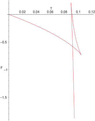
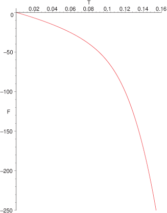
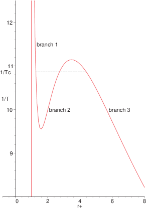
FIG. 5.: The first two graphs show the free energy vs. temperature for the fixed charge ensemble. The situation for $q{<}q_{\rm crit}$ and $q{\geq}q_{\rm crit}$, respectively, are plotted. (The values $n{=}4$, $G{=}1$, $l{=}5$ and $q{=}1,25$ have been used here.) The first graph is the union of three branches. Branch 1 emanates from the origin, and merges with branch 2 at a cusp. Branch 3 forms a cusp with the other end of branch 2, and continues towards the bottom right. The graph on the right shows how the branches arise from the inverse temperature curves of eqn. (24). (See text for discussion of critical temperature $T_{c}$.)

That there are three branches for the small charge case follows from the second graph in figure 3, which is magnified and labeled in fig. 5, on the right. From there, it is clear that for low temperature there can only be one solution (“branch 1”) for the black hole radius. At some temperature $T_{1}{=}1/\beta_{1}$, the origin of two new branches (“branches 2 and 3”) of solutions appears ($T_{1}{=}0.089,\beta_{1}{=}11.15$ for the chosen parameters in the plot.). Above this temperature (below $\beta_{1}$), there are therefore three distinct branches of solution until at temperature $T_{2}{=}1/\beta_{2}$, ($T_{2}{=}0.105,\beta_{2}{=}9.55$ in the plot) two of the branches (1 and 2) coalesce and disappear, leaving again only a single branch (3), which persists for all higher temperatures.

Returning to the free energy plot, the meaning is now clear. Starting to the extreme left of the plot, (low temperature) we see that there is a single branch of free energy, corresponding to the branch 1 solutions. At $T_{1}$, branches 2 and 3 appear on the graph and separate from each other at higher temperatures. At $T_{2}$, branches 1 and 2 coalesce and disappear, while branch 3 persists for all higher temperatures, continuing to the left.

So from zero temperature the negative free energy of branch 1 means that those non–extreme black holes dominate the thermodynamic ensemble. At temperature $T_{c}$, ($T_{c}{=}0.092$ in the plot) the free energy of branch 3 is actually more negative than that of branch 1, and so that branch of non–extremal black holes takes over the physics and continue to do so for all higher temperatures.

The situation at $T_{c}$ is a genuine finite temperature phase transition, of first order. (Notice from the first graph in figure 5 that the free energy is continuous, but its first derivative is discontinuous.) This results from the jump (along the dotted line in the final graph in figure 5) from branch 1 to branch 2, from small to large $r_{+}$ black holes, as the temperature increases. As the entropy is proportional to $r_{+}^{n-1}$, there is a jump in the entropy, or a release of “latent heat”.

As we approach the critical value, $q_{\rm crit}$, of the charge representing the crossover into the large charge regime, the kink in the free energy —and therefore the transition— vanishes, as branches 1 and 3 merge (and branch 2 disappears). The difference in horizon radii between the two branches, $\rho_{+}{=}r^{(3)}_{+}{-}r^{(1)}_{+}$, may be thought of as an order parameter for the transition, as it vanishes above $q_{\rm crit}$, where the transition goes away.

As noted before in the case of fixed potential ensemble, branches 2 and 3 are the exact analogues of the small and large Schwarzschild black holes of Hawking and Page[6], or the small and large Taub–bolts discovered in the thermodynamic studies of ref. [7, 30]. In those papers, above a certain temperature $T_{1}$, there were two allowed solutions at a given temperature, the smaller (branch 2) being unstable and the larger (branch 3) being stable, which persists to dominate the thermodynamics above some critical temperature $T_{c}$. The existence of a stable branch 1, and its merger with branch $2$ to disappear at $T_{2}$ is a new feature when we add a small fixed charge to the story. Conversely, if we start from a situation where charge is present on the black hole but the cosmological constant vanishes, then we find branches 1 and 2, and it is only when the negative cosmological constant is turned on that branch 3 appears.

For large charge, there is only a single branch allowed, (see figure 5, the cusps collide and disappear) and the associated thermodynamic story is correspondingly simpler. The free energy shows that the non–extreme charged black holes dominate from $T{=}0$.

In all cases (large or small $Q$), the ultra high temperature phases are dominated by a black hole and the free energy and entropy have the characteristic “unconfined” field theory behaviour shown in eqns. (34).

One might examine the approach to the critical point more closely. In particular, consider the behaviour of the specific heat

$$c_{q}\equiv{\partial M\over\partial T}={\partial M/\partial r_{+}\over\partial T/\partial r_{+}}\ .$$ (36)

With $q{=}q_{\rm crit}$, as the temperature approaches the critical value, one finds a singularity with $c_{q}{\propto}(T{-}T_{c})^{-2/3}$. This behavior may be contrasted with the $(T{-}T_{c})^{-1/2}$ singularity found in ref.[23]. The essential difference is of course that near the critical point we have a point of inflection with $T{-}T_{c}\propto(r_{+}{-}r_{\rm crit})^{3}$, while ref.[23] considers a minimum with $T{-}T_{c}\propto(r_{+}{-}r_{\rm crit})^{2}$.

The evolution of the free energy of the system as a function of charge is particularly interesting as one goes from zero charge to large charge. The single cusp of the uncharged (Schwarzschild) system is joined by a second cusp which comes in from infinity, forming (with the original one) a section of the well known “swallowtail” shape, familiar as a bifurcation set or “catastrophe” in singularity or catastrophe theory. The significance of this is discussed in the next section. As we cross over into the large charge regime at some critical value of $q$, the cusps merge and the free energy becomes a simple monotonic function. For completeness, we include a series of plots showing this evolution. (We do not put them on the same axes, as we did for the fixed potential case, for the sake of clarity.)

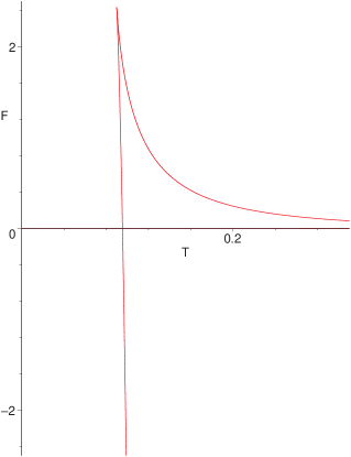
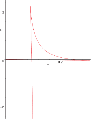
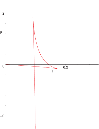
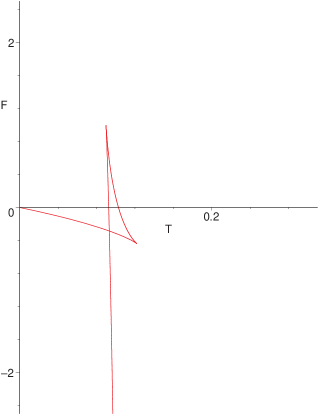
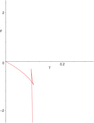
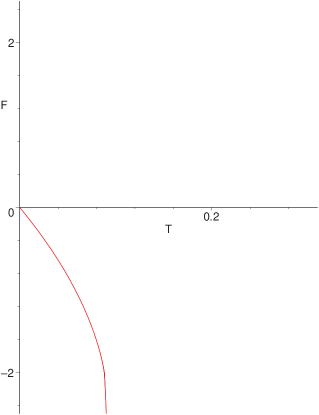
FIG. 6.: The free energy vs. temperature for the fixed charge ensemble, in a series of snapshots for varying charge, starting from (near) zero charge (top left) and finishing with large charge (bottom left). The values $l{=}5$, $G{=}1$, and $n{=}4$ are used here. This complete evolution describes the two dimensional“swallowtail” catastrophe.

The resulting thermodynamic phase structure for the fixed charge ensemble is summarized in the diagram on the right in figure 1.

VI Catastrophic Holography?

We cannot refrain from further general comments upon the meaning and structure of the curves that we have uncovered in the previous sections. Although we plotted only the cases for the $n{=}4$ case, representing AdS₅ (and hence four dimensional field theory), the same universal structures appear in the cases $n{=}3$ and 6 as well, giving the same pleasing phase structure for the fixed charge ensemble.

The phase structure that we uncovered for the fixed charge ensemble should remind the reader of the classic van der Waals–Maxwell behaviour, modeling the liquid–gas system. Indeed, they are isomorphic. The $\beta(r_{+})$ curve (the middle graph of figure 3) should recall the graph of the $P(V)$ van der Waals equation of state, where $P$ (the pressure) is replaced here by $\beta$ and $V$ (volume) by $r_{+}$.

The instability of branch 2 is then simply the familiar instability of the corresponding section of the van–der Waals curve. The jump from branch 1 to branch 3 which we deduced from the form of the free energy is the precise analogue of the Maxwell construction. In the isomorphism between our parameters and those of the van der Waals–Maxwell system, our charge $Q$ is equivalent to their temperature $T$.

The instability of branch 2 in both languages makes intuitive sense: as one increases the pressure, the volume should decrease, and therefore the positively sloped branch is not stable. A similar statement holds for the black holes after making the translation to the current situation: For black holes in equilibrium with the heat bath, an increase in the temperature results in an increase in the black hole radius and hence mass, for stable black holes. Notice that this also follows from the first law, recalling that the entropy is a positive power of the radius. So the positive slope branch of the $\beta(r_{+})$ curve is generally unstable.

In the language of catastrophe theory[34] —the study of jumps in some “state variables” as a result of smooth changes in “control variables”— the physical solutions of the $\beta(r_{+},q)$ curve, viewed as a two dimensional surface in $(\beta,q,r_{+})$ space, is the “control surface” of the “cusp catastrophe”. The cusp shape is the union of points in the $(\beta,r_{+})$ plane (the control variables) where the state variable (the allowed value of $r_{+}$) jumps from branch 1 to branch 3, as branch 2 is unstable. After applying the minimum free energy condition to determine the allowed branches (the “Maxwell criterion”), the cusp catastrophe appears in the $(q,\beta)$ plane, (or equivalently the $(Q,T)$ plane) collapsed to the critical line (see figure 1) (or “vapour pressure curve”) along which the two types of black hole can coexist, and across which there is a phase transition. The end of the line, at the critical value $q_{\rm crit}$, where branch 2 disappears, is the point where the distinction between branch 1 and 3 goes away. The order parameter, $\rho_{+}$ for this critical point is the radius difference of the branches $\rho_{+}{\equiv}r^{(3)}_{+}{-}r^{(1)}_{+}$. Beyond the critical charge there is no phase transition ($\rho_{+}{=}0$) in going from branch 1 black holes to branch 3 by increasing the temperature. This is of course the familiar statement that above a critical temperature, there is no phase transition in going from a gas to a liquid by increase of pressure.

Intriguing is the fact that the two dimensional free energy surface $F(\beta,Q)$ forms the shape of the swallowtail catastrophe (see figure 6). (Note that for $n{=}3,4$ and $6$ the shape is the same.) This naturally follows from the ability of the $\beta(r_{+})$ curve to produce three branches, and the resulting shape for the free energy curve is the union of three branches.

Here, the swallowtail does not have the usual interpretation as a bifurcation surface (like the cusp does above) but it is natural to wonder whether its appearance tells us that there is some universality at work here. This is because the language of catastrophe theory is largely a classification of the possible distinct types of bifurcation shapes that can occur. This classification (which, for the common “elementary” cases is of A–D–E type) is equivalent to the (perhaps more familiar) classfication of singularities[35]. A natural question is whether or not the inclusion of more control parameters will always result in a free energy curve of a shape (and corresponding phase structure) which falls into the classification. It would certainly be amusing to find yet another case of the A–D–E classification appearing in string and M–theory physics.

VII Concluding Remarks

The study of the thermodynamics of black holes in Einstein–Maxwell–anti–deSitter is highly relevant to the thermodynamics of certain superconformal field theories with a background global current switched on. This follows from the logic of the AdS/CFT correspondence, and the fact that the EMadS system can arise as the near–horizon physics of rotating M2– and D3–branes, and it should therefore be regarded as the effective theory of the strongly coupled field theory living on the rotating branes’ world–volume.

The phase structures of the charged black hole systems studied here, and summarized in figure 1, are markedly different from those of the uncharged systems studied before in this context [3, 4, 6, 7]. The addition of charge revealed a rich phase structure, with precise analogues to classic thermodynamic systems. The physics is consistent with a dual field theory interpretation.

In all cases, the infinite volume limit can be found by taking the limits given in eqn. (18). This scaling may be applied to the expressions for the actions (eqns. (23) and (27)) and the period (eqns. (24) and (25)). In all cases, the result is that there is only one branch of black hole solutions (like the large charge and potential situations had in finite volume), and the free energy is negative definite, showing that the thermodynamics is dominated by black holes for all temperatures. Of course, this is what we should expect, from the field theory point of view.

As we commented before, the gauge field in the AdS space naturally couples to a CFT current $J_{\mu}$, following the prescription of ref. [3]. From the asymptotic variation of the gauge field (12) or its corresponding field strength, one then has an expectation value $\langle J_{t}\rangle{\sim}q$. Thus one might think of the CFT state as containing a plasma of (globally) charged quanta. The precise nature of the CFT state depends on the ensemble, which we were studying. For the case of the fixed potential, the dual statement is that a chemical potential conjugate to the global charge has been introduced leading to the expectation value. The fixed charge calculations correspond to an ensemble of CFT states with a fixed global charge. Thus the difference between the two calculations is analogous to that between the canonical (fixed $T$) and microcanonical (fixed $E$) ensembles.

In the context of D3 branes with $n{=}4$, the $SO(6)$ gauge fields couple to the R–symmetry currents in the super–Yang–Mills theory. This aspect of the duality has been used to great advantage to produce nontrivial consistency tests by comparing correlators protected by supersymmetry[33]. Of course in the present case, with the truncation to EMadS theory, we are focussed on a particular diagonal $U(1)$ generator of the $SO(6)$ symmetry.

In this context, we can translate the results of the supergravity calculations to quantitative statements about the strong coupling behavior of the super–Yang–Mills theory. Up to numerical factors, we have as usual[1]: $g^{2}_{YM}{\sim}g$ and $(l/l_{s})^{4}{\sim}gN$, (where $g$ is the type IIB string coupling) as well as $G_{5}{\sim}g^{2}l_{s}^{8}/l^{5}$. It remains fix how the black hole charge should be characterized in the CFT. The most natural approach is to measure the physical charge (11) in terms of the fundamental charge of the Kaluza–Klein excitations in the AdS space, i.e., with $Q{=}{\bar{Q}}/l$. In the field theory then, ${\bar{\rho}}{=}\bar{Q}/V_{3}$ (where $V_{3}$ is the spatial volume of the field theory) essentially counts the number of fundamentally charged quanta per unit volume in a given state. Given this framework, we can consider the field theory content of our results. For example, one might wonder what the critical charge (29) appearing in the fixed charge phase diagram corresponds to:

$${\bar{Q}}_{\rm crit}\sim{l\,q_{\rm crit}\over G_{5}}\sim N^{2}.$$ (37)

In general, translating the entropy, mass or free energy to a field theory expression produces a complicated function of both the temperature $T$ and the charge $\bar{Q}$. One relatively simple case is the high temperature limit, where the charge essentially plays no role (see eqn. (34)). Another interesting case to consider is that of the extremal black holes for which $T{=}0$. By demanding that $V(r_{+}){=}0$ and $(\partial V/\partial r)(r_{+}){=}0$ have a consistent solution, one finds that the mass and charge parameters are related by the following expression:

$$\sqrt{z^{2}-y^{2}}=(1+z)-\sqrt{1+z},$$ (38)

where $z{=}3m/l^{2}$ and $y^{2}{=}27q^{2}/l^{4}$. A simple case to consider is that of a large black hole with $m{>>}l^{2}$, for which $z^{3}{\simeq}y^{4}/4$. Further in this limit, one has that $m{\sim}r_{+}^{2}$ and so

$$S\sim{r_{+}^{3}\over G_{5}}\sim{l\,q\over G_{5}}\sim V_{3}{\bar{\rho}}\sim{\bar{Q}}.$$ (39)

Notice that implicitly here we are considering a regime where ${\bar{Q}}{>>}N$. The lack of dependence of the entropy on $N$ is a signal of confined behaviour at zero temperature, despite the presence of the black hole. It would certainly be interesting if this entropy result could be recovered by considering partitioning of the charge $\bar{Q}$ amongst the charged excitations of the CFT.

We have left aside the case of compactification of six dimensional supergravity on $S^{3}$ to get AdS₃. By setting the $S^{3}$ in rotation in its two independent rotation planes, in a symmetric fashion, we get an electric potential in AdS₃. Doing so, notice that if we start from the solution describing a rotating six dimensional black string (such as the one obtained from the D1–D5 bound state), then, in the throat limit the rotation of the $S^{3}$ can be undone by a diffeomorphism[31]. In other words, the effective gauge field in three dimensions is pure gauge. Nevertheless, as shown in ref.[32], there do exist charged black hole solutions in EMadS theory in three dimensions. These have an electric potential that diverges logarithmically at infinity, which prevents one from defining the ensemble at fixed potential. Nevertheless, if the extremal black hole background is subtracted, then the fixed charge ensemble can be appropriately defined. For non–rotating black holes (in ref.[32], the full Kerr–Newman solution is constructed) there is only one branch, just like we have found for large fixed charge (see figure 3, left), with corresponding simple thermodynamic structure given by figure 4 (left).

Finally, it is also worth remarking that the close similarity that we have observed with familiar structures from equilibrium thermodynamics, and expectations from a dual field theory is further encouragement (for those who need it) that the quantum mechanics of black holes is not unlike that of other situations.

References

References

- [1] J. Maldacena, Adv. Theor. Math. Phys. 2 (1998) 231, hep-th/9711200
- [2] S. S. Gubser, I. R. Klebanov, and A. M. Polyakov, Phys. Lett. B428 (1998) 105, hep-th/9802109.
- [3] E. Witten, Adv. Theor. Math. Phys. 2 (1998) 253, hep-th/9802150.
- [4] E. Witten, Adv. Theor. Math. Phys.2 (1998) 505, hep-th/9803131.
-
[5]
G. ’t Hooft, gr-qc/9310026;
L. Susskind, J. Math. Phys. 36 (1995) 6377, hep-th/9409089. - [6] S.W. Hawking and D.N. Page, Commun. Math. Phys. 87, 577 (1983).
- [7] A. Chamblin, R. Emparan, C. V. Johnson and R. C. Myers, Phys. Rev. D59, 064010 (1999) hep-th/9808177.
- [8] R. Penrose, Nuovo Cimento 1 (1969) 252.
-
[9]
A.A. Starobinsky, J.E.T.P. 37 (1973) 28;
W. Unruh, Phys. Rev. D10 (1974) 3195;
N. Deruelle and R. Ruffini, Phys. Lett. 52B (1974) 437; ibid., 57B (1975) 248. -
[10]
G. Denardo and R. Ruffini, Phys. Lett. 45B (1973) 259;
T. Damour and R. Ruffini, Phys. Rev. Lett. 35 (1975) 463. - [11] G.W. Gibbons, Commun. Math. Phys. 44 (1975) 245.
- [12] S.W. Hawking, M.M. Taylor-Robinson, Phys.Rev. D55 (1997) 7680, hep-th/9702045.
- [13] D.N. Page, Phys. Rev. D14 (1976) 3260.
- [14] J. D. van der Waals, Phd. Thesis, University of Leiden (1873).
-
[15]
See, for example R. M. Wald, Ann. Phys. 82 (1974)
548;
R.M. Wald, “General Relativity”, The University of Chicago Press, Chicago (1984);
R.M. Wald, “Quantum field theory in curved space–time and black hole thermodynamics”, The University of Chicago Press, Chicago (1994);
N.D. Birrell and P.C.W. Davies, “Quantum fields in curved space”, Cambridge University Press, Cambridge (1982);
P. R. Brady, I. G. Moss, R. C. Myers, Phys. Rev. Lett. 80 (1998) 3432, gr-qc/9801032. - [16] J. Louko and S.N. Winters-Hilt, Phys.Rev. D54 (1996) 2647, gr-qc/9602003.
- [17] R.C. Myers and M.J. Perry, Ann. Phys. 172 (1986) 304.
- [18] L.J. Romans, Nucl. Phys. B383, 395 (1992); hep-th/9203018.
- [19] L.A.J. London, Nucl. Phys. B434, 709-735 (1995).
-
[20]
L.F. Abbott and S. Deser,
Nucl. Phys. B195, 76 (1982)
S.W. Hawking and G.T. Horowitz, Class. Quant. Grav. 13, 1487 (1996). -
[21]
K. Behrndt, A.H. Chamseddine and W.A. Sabra, Phys. Lett.
B442 (1998) 97, hep-th/9807187;
K. Behrndt, M Cvetic and W.A. Sabra, hep-th/9810227. -
[22]
J.G. Russo, hep-th/9808117;
C. Csaki, Y. Oz, J.G. Russo and J. Terning, Phys. Rev. D59 (1999) 065008, hep-th/9810186;
P. Kraus, F. Larsen and S.P. Trivedi, hep-th/9811120;
J.G. Russo and K. Sfetsos, hep-th/9901056. -
[23]
S.S. Gubser, hep-th/9810255;
R.G. Cai and K.S. Soh, hep-th/9812121. -
[24]
R.B. Mann,
Class. Quant. Grav. 14, L109 (1997)
gr-qc/9607071.
D.R. Brill, J. Louko and P. Peldan, Phys. Rev. D56, 3600 (1997) gr-qc/9705012.
L. Vanzo, Phys. Rev. D56, 6475 (1997) gr-qc/9705004. - [25] R. Emparan, Phys. Lett. B432, 74 (1998) hep-th/9804031.
-
[26]
S. Sethi and L. Susskind,
Phys. Lett. B400, 265 (1997)
hep-th/9702101.
T. Banks and N. Seiberg, Nucl. Phys. B497, 41 (1997) hep-th/9702187.
E. Witten, hep-th/9507121.
A. Strominger, Phys. Lett. B383, 44 (1996) hep-th/9512059
For a review, see N. Seiberg, Nucl. Phys. Proc. Suppl. 67, 158 (1997) hep-th/9705117. -
[27]
M. J. Duff and J. T. Liu,
hep-th/9901149;
M.M. Caldarelli and D. Klemm, hep-th/9809097;
D. Klemm, hep-th/9810090 (to appear in Nucl. Phys. B). -
[28]
G.W. Gibbons and R.E. Kallosh, Phys. Rev. D51
(1995) 2839, hep-th/9407118;
S.W. Hawking, G.T. Horowitz and S.F. Ross, Phys. Rev. D51, 4302 (1995) gr-qc/9409013;
S.W. Hawking and Gary T. Horowitz, Class. Quant. Grav. 13 (1996) 1487, gr-qc/950101;
C. Teitelboim, Phys. Rev. D51 (1995) 4315, hep-th/9410103. -
[29]
H.W. Braden, J.D. Brown, B.F. Whiting and J.W. York,
Phys. Rev. D42, 3376 (1990);
S.W. Hawking and S.F. Ross, Phys. Rev. D52, 5865 (1995) hep-th/9504019. - [30] S.W. Hawking, C.J. Hunter and D.N. Page, Phys. Rev. D59, 044033 (1999) hep-th/9809035.
-
[31]
M. Cvetic and F. Larsen,
Nucl. Phys. B531, 239 (1998)
hep-th/9805097;
J.P. Gauntlett, R.C. Myers and P.K. Townsend, Phys. Rev. D59, 025001 (1999) hep-th/9809065. - [32] M. Bañados, C. Teitelboim and J. Zanelli, Phys. Rev. Lett. 69, 1849 (1992) hep-th/9204099.
- [33] D.Z. Freedman, S.D. Mathur, A. Matusis and L. Rastelli, hep-th/9804058.
- [34] See for example, R. Gilmore and R. Knorr, “Catastrophe Theory for Scientists and Engineers”, Dover, 1993.
- [35] See for example, V. I. Arnold, “Singularity Theory: Selected Papers”, (London Math. Soc. Lecture Note Series 53, (Cambridge 1981).