Boundary Conformal Field Theories, Limit Sets of Kleinian Groups and Holography

Abstract

In this paper, based on the available mathematical works on geometry and topology of hyperbolic manifolds and discrete groups, some results of Freedman et al (hep-th/9804058) are reproduced and broadly generalized.Among many new results the possibility of extension of work of Belavin,Polyakov and Zamolodchikov to higher dimensions is investigated. Known in physical literature objections against such extension are removed and the possibility of an extension is convinsingly demonstrated

1. Introduction

Recently, there had been attempts to extend the results of two dimensional conformal field theories(CFT) to higher dimensions $[1.2].$ Since publication of papers by Witten$[3,4]$it had become clear that there is a very close correspondence between 2d physics of critical phenomena and 3d physics of knots and links. A very detailed study of this correspondence is developed by Moore and Seiberg $[5]$. Additional contributions more recently were made in Ref[6], etc. All these works heavily exploit the algebraic aspects of this correspondence through use of Yang-Baxter equations, quantum groups, etc. Much lesser efforts had been spent on development of the same correspondence from the topological point of view through study of 3-manifolds complementary to knots(links) in $S^{3}$=$R^{3}\cup\{\infty\}.$ Such study is potentially more beneficial since it is known $[7]$ that in four dimensions all knots are trivial (i.e.unknotted) so that the algebraic methods used so far are necessarily limited to 3 dimensions and, accordingly, to study of two dimensional CFT only. At the same time, topological study of manifolds is not limited to three dimensions. The reasons why such studies are useful could be understood from the following simple arguments taken from the book by Maskit $[8].$

Define an inclusion of $R^{d}$ into $R^{d+1}$ through $R^{d}$ ={(x,t)$\mid t=0\}$ where x$\in R^{d},-\infty\leq t\leq\infty.$ The upper half space Poincar$e^{\prime}$ model of hyperbolic space H^d+1is defined by

$$\text{H}^{d+1}=\{(x,t)\mid t>0\}$$ (1.1)

with $x\in R^{d}$ so that $\partial$H${}^{d+1}=R^{d}$. Consider a special group G of motions G=M^d+1 of $R^{d+1}=\{x,t\}$ made of

a) translations:  (x,t)$\rightarrow(x+a,t)$ ,$a\in R^{d-1\text{ }};$

b) rotations :  (x,t)$\rightarrow$ (r(x),t) , r$\in O(d-1);$

c) dilatations :  x$\rightarrow\lambda x$ ,$\lambda>0,\lambda\neq 1$ and

d) inversions :  x$\rightarrow\frac{x}{\left|x\right|^{2}}$ .

It can be proven$[8]$ that the group G acts as a group of isometries of H^d+1and is called d dimensional M$\ddot{o}$bius group. In its action on R^d ”G acts as a group of conformal motions but not as a group of isometries in any metric”.

At the same time, it is well established$[9]$ that in any dimension the physical system at criticality possesses the invariance which is described in terms of the group G. Hence, the very existence of criticality is closely associated with the hyperbolicity of the adjacent space.

Let x$\in H^{d+1}$ and $\gamma\in$G. Consider a motion (an orbit) in H^d+1 by successive applications of $\gamma$ to x. It is of interest to study if such a motion will ever hit $\partial$H${}^{d+1}=R^{d}$. This problem is highly nontrivial and was solved by Beardon and Maskit$[10]$ (e.g.see section 5 below for more details) for d=2. The nontriviality of this problem could be better understood if, instead of the upper half space H^d+1model, we would consider the unit ball B^d+1 model of the hyperbolic space with the unit sphere $S_{\infty}^{d}$ $($sphere at infinity) playing the same role as in this model as $\partial$H${}^{d+1}=R^{d}$ in the upper half space model. Since not all subgroups of G will allow hitting of the boundary, it is clear, that one should be interested only in those subgroups whose orbits end up at the boundary. These subgroups, in turn, could be further subdivided into those whose limit points on $S_{\infty}^{d}$ will cover the entire sphere and those which will cover only a part of $S_{\infty}^{d}$. This part we shall denote as $\Lambda.$ The limit set $\Lambda$ is actually a fractal . The fractal dimension of $\Lambda$ is directly related to the critical indices of the two-point correlation functions of the corresponding conformal models at criticality. Different subgroups of M$\ddot{o}$bius group G will produce different fractal dimensions. In turn, the corresponding hyperbolic manifolds associated with these groups could be viewed as complements of the related knots (links) in the case of 2+1 dimensions so that different conformal models, indeed, could be associated with different types of knots(links). This association becomes unnecessary when one is interested in conformal models in dimensions 3 and higher. One could still consider motions associated with subgroups of M$\ddot{o}$bius group and the corresponding, say, hyperbolic 4-manifolds without using knots, braids, Yang-Baxter equations, etc.

Although stated in different form, recent results of Maldacena$[11]$ and their subsequent refinements in Refs[12-16] (and many additional references therein and elsewhere which we do not include) are actually directly connected with ideas just described. In physics literature the connection between ”surface” and ”bulk” field theories is known as holographic principle (holographic hypothesis)[17,18]. In simple terms [19], it can be formulated as statement that ”a macroscopic region of space and everything inside it can be represented by a boundary theory living on the boundary region”. Mathematical support of this principle in physics literature is attributed to works by Fefferman and Graham [20] and Graham and Lee[21]. These works discuss  boundary conditions at infinity for Einstein manifolds (spaces) and initial value problem for Einstein’s equations. Although our previous discussion did not involve the Einstein manifolds, actually, the results of Ref.[21] are consistent with those which follow from the hyperbolic geometry. This can be understood if one takes into account that Einstein spaces are characterized by the property that the Ricci tensor $R_{ij}$ is proportional to the metric tensor $g_{ij}$ [22], that is

$$R_{ij}=\lambda g_{ij}.$$ (1.1)

Since the scalar curvature $R=g^{ij}R_{ij}$ , the above equation can be rewritten as

$$R_{ij}=\frac{R}{d}g_{ij}$$ (1.2)

where d is the dimensionality of space (as before). The Einstein tensor

$$G_{j}^{i}=R_{j}^{i}-\frac{1}{2}\delta_{j}^{i}R$$ (1.3)

acquires a particularly simple form with help of Eq.(1.2):

$$G_{j}^{i}=(\frac{1}{d}-\frac{1}{2})\delta_{j}^{i}R$$ (1.4)

and, because $G_{j,h}^{i}$ =$0$, we obtain,

$$(\frac{1}{d}-\frac{1}{2})R\text{ ,}_{j}=0.$$ (1.5)

This implies ,that the scalar curvature $R$ is constant . For isotropic homogenous spaces E_d the Riemann curvature tensor is known to be[23] given by

$$R_{ijkl}=k(x)(g_{ik}g_{jl}-g_{il}g_{jk})$$ (1.6)

so that the Ricci tensor  is  given by

$$R_{ij}=(d-1)k(x)g_{ij},$$ (1.7)

where k(x) is the sectional curvature at  the point x$\in$E_d . The Schur’s theorem[23] guarantees, that $k(x)=k=const$ for $d\geq 3$ .Comparison between Eqs.(1.1) and (1.7) produces then : $\lambda=(d-1)k$ and, accordingly, $R=d(d-1)k$ . The spatial coordinates can always be rescaled so that, for $k<0$ we obtain, the canonical value $k=-1$ characteristic of hyperbolic space[24,25] . Since  in the work by Graham and Lee [21] the condition given by Eq.(1.7) is used (with $k=-1$), the connections with hyperbolic geometry  is evedent. Since Eq.(1.4) can be equivalently rewritten with help of Eq.(1.7) as

$$R_{ij}-\frac{1}{2}g_{ij}R+\hat{\Lambda}g_{ij}=0,$$ (1.8)

with the cosmological term $\hat{\Lambda}$ =-$\frac{1}{2}(d-1)(d-2),$thus obtained equation produces metric for Einstein space  known in literature as anti-de Sitter (AdS) space[26]. Hence, in part, the purpose of this work is to investigate in some detail connections between the results obtained in physics literature and related to CFT-AdS correspondence, e.g.see Ref.[12], and those known in mathematics those known in mathematics and related to hyperbolic geometry and hyperbolic spaces. Not only it is possible to reobtain results known in physics using these connections, but many more follow along the way of physical reinterpretation of known results in mathematics. Establishing these connections touches many aspects of modern mathematics such as the geometry and topology of hyperbolic manifolds$[25]$, multidimensional extension of the theory of Teichmüller spaces$[27],$ spectral analysis of hyperbolic manifolds$[28]$ (including those with cusps$[29])$, random walks on group manifolds$[30]$, theory of deformations of Kleinian and Fuchsian groups$[31]$(and M$\ddot{o}$bius groups in general), ergodic theory of discrete groups$[32]$, Kodaira-Spencer theory of deformations of complex manifolds$[33]$, loop groups$[34],$cohomology of groups, etc. In particular, the cohomological aspects of these connections lead directly to the Virasoro algebra and its generalizations thus allowing us to dicuss the extension of fundamental results of Belavin-Polyakov-Zamolodchikov(BPZ) [35] to higher dimensions(e.g.see section 8). To make our presentation self-contained, we had incorporated some the auxiliary results from mathematics into text which are meant only to facilitate reader’s understanding without detracting of his/her attention from physical goals and motivations of this work. A quick summary of some auxiliary mathematical results related to hyperbolic 3-manifolds and Einstein spaces also could be found in our papers, Ref.s[36,37].

This paper is organized as follows. In section 2 we discuss an auxiliary Plateau problem in d+1 dimensional Euclidean space. Already in two dimensions the full analysis of the Plateau problem is quite nontrivial as it was demonstrated in classical work of Douglas published in 1939 $[38]$. Multidimensional treatment of this problem is even more nontrivial and touches many subtle aspects of the harmonic analysis $[39].$ Nevertheless, the extension of the Euclidean variant of the Plateau problem to the hyperbolic H^d+1space is actually not difficult and was accomplished rather long time ago by Ahlfors$[25]$. Using the results of Ahlfors we were able to reobtain the results of Freedman et al, Ref.[12], almost straightforwardly in section 3. We deliberately considering only the scalar field case in this work since the extension of our treatment to vector and tensor fields (to be briefly considered in Section 8 ) does not cause much additional conceptual problems. To generalize the results of section 3 and to put them in an appropriate mathematical context, we discuss (in section 4) diffusion in the hyperbolic space. This is done with several purposes. First, using symmetries of the Laplace operator acting in the hyperbolic space it is possible to subdivide Brownian motions on transient and recurrent. Only transient motions can reach the boundary of the hyperbolic space. The transience and/or recurrence is associated with convergence /or divergence of certain infinite sums known as Poincar$e^{\prime}$ series.The convergence or divergence of such series is being controlled by the critical exponent $\alpha.$ Patterson$[40]$, Sullivan$[41]$, Ahlfors[25], Thurston $[42]$ and others $[32]$ had shown that this exponent is associated with the fractal dimension of the limit set $\Lambda.$ Stated in physical terms, it is shown in section 5 that this exponent is associated with the exponent 2$\nu$ for the two-point correlation function of the corresponding boundary CFT . The exponent $\alpha$ depends upon the specific group of motions in H^d+1. This group is directly associated with the hyperbolic manifold so that different groups associated with different manifolds will produce different $\alpha^{\prime}s.$ Being armed with these ideas it is possible to improve the existing physical results using spectral theory of hyperbolic manifolds in section 6. In this section it is shown that the obtained eigenvalue spectrum of the hyperbolic Laplacian discussed in physics literature is incomplete and much more results could be obtained with help of the existing mathematical literature, e.g.see Ref.[28]. For instance, 2d critical exponent 2$\nu$ for the Ising model is almost straightforwardly obtained with help of the recently obtained results of Bishop and Jones$[43]$ .With this result obtained, it is only natural to look for connections between the boundary CFT results and those coming from the fundamental work of BPZ$[35]$ .The connection can be established rather easily,e.g.see section 7 ,based on the theory of deformation of Kleinian groups$[27,31]$ which is closely associated with the theory of Teichmüller spaces$[44]$ as it was demonstrated by Bers$[45]$ some time ago. One of the sources which generates ”new” Kleinian groups from the ”old” ones is through the extension of the quasiconformal deformations produced at the boundary $\Omega=S_{\infty}^{2}-\Lambda$ of the hyperbolic space into the bulk(i.e.holography in physical terminology). The theory of such deformations was under development in mathematics for quite some time. However, the results which are essential for making connections with current physics literature had been obtained by mathematicians only quite recently. In particular, Canary and Taylor$[46]$ had demonstrated that the limit set of Kleinian groups which produce critical exponents $\alpha$ in physically interesting range (e.g. for 0$<$$\alpha<1$ one obtains the correct Ising model critical exponent 2$\nu=1/4,etc.)$ is a circle $S$, perhaps, with some points(or, may be, segments) being removed (e.g. see section 7 for more details). These facts naturally explain the crucial role being played by the loop groups and the loop algebras$[34]$ in the conformal field theories and other exactly integrable systems [47]. At the same time, Nag and Verjovsky$[48]$ had demonstrated how the boundary deformations of such circle is connected with the central extension term of the Virasoro algebra thus providing major physical reasons for existence of such term. Moreover, the analysis of the seminal work by Nag and Verjovsky indicates that, actually, their main results are based entirely on much earlier work by Ahlfors[49] . The Virasoro algebra and all results of the CFT [$35]$ could be obtained much earlier should work by Ahlfors$[49],$ written in 1961, be properly interpreted at that time. Ahlfors and many others (e.g.see Ref. [27] for a review) had developed extension of theory of  2 dimensionalquasiconformal deformations to hyperbolic spaces of higher dimensions. When these results are being put in a proper physical context they allow extension of the BPZ formalism to higher dimensions. The possibility of such extension(s) is discussed in section 8. Taking into account that the conformal group in d dimensions is isomorphic to the Lie group O(d+1,1) as noticed by Cartan in 1920’s [50], for d=2 we obtain the Lie group O(3,1) known also as Lorentz group. The connected part of this group is isomorphic to $PSL(2,C)$ [51]. The Lie algebra of this group lies in the center ($VectS^{1})$ of the Virasoro algebra . The central extension of this algebra is just the Virasoro algebra. For d=3  we have the Lie group O(4,1) known as de Sitter group. The representations of the Lie algebra for this group ,fortunately, were studied both in mathematics [52,53] and in physics[54,55] in connection with exact algebraic solution of the hydrogen atom.Since the hydrogen atom is exactly solvable quantum mechanical problem, construction of representations of the Lie algebra for the de Sitter Lie group is also known. It is facilitated by the major observation[52,53] that the Lie algebra of the de Sitter group can be presented as direct tensor product  of the Lie algebras for the group SO(3)$\simeq PSL(2,C).$ Hence, it is possible to construct the central extensions for each of the Lie algebras so(3) independently thus forming two copies of Virasoro algebras with different central charges in general. Construction of the tensor products of  Virasoro algebras had been discussed in the literature already (e.g. see Lecture 12 of Ref.[56]). This possibility is worth discussing only if the limit set $\Lambda$ is union of two independent circles. Since this fact had not been proven, to our knowlege, other possibilities also exist, e.g. $\Lambda$ is still a circle. These possibilities are discussed briefly in the same section. Recently, Bakalov, Kac and Voronov[57] were able to extend the cohomological analysis of Gelfand and Fuks[58]  thus obtaining the higher dimensional analogue of the Virasoro conformal algebra (e.g. see section 10 of Ref.[57]). It remains a challenging problem to recover these results by developing the Kodaira-Spencer-like cohomological theory of multidimensional quasiconformal deformations. Some efforts in this direction are mentioned in the same section.

2.  The Plateau problem in d+1 dimensional Euclidean space

The classical Plateau problem, when stated mathematically, essentially coincides with the Dirichlet problem. In two dimensions the Dirichlet problem can be formulated as follows:among functions $\varphi(z)$, z $\in A$ (where $A$ is some closed domain of the complex plane $\mathbf{C)}$ which take values $\varphi_{0}(z)$ at $\partial A$ find such that the Dirichlet integral $D$[$\varphi]$ defined by

$$D[\varphi]=\iint\limits_{A}d^{2}z(\vec{\nabla}\varphi\cdot\vec{\nabla}\varphi)$$ (2.1)

has the lowest possible value. Evidently, the above problem can be reduced to the problem of finding the harmonic function $\varphi(z)$, i.e. the function which obeys the Laplace equation

$$\Delta\varphi=0\text{ if z}\in A\text{ but z}\notin\bar{A}$$ (2.2)

and takes at the boundary $\partial A$ the preassigned values

$$\varphi\mid_{\partial A}=\varphi_{0}(z)\text{ .}$$ (2.3)

If $G(z,z^{\prime})$ is the Green’s function of the Laplace operator $\Delta$, then the harmonic function which possess the above properties is given by the following boundary integral

$$\varphi(z)=-\int\limits_{\partial A}d\sigma\varphi_{0}(\sigma)\frac{\partial G}{\partial n}$$ (2.4)

with normal derivative taken with respect to the direction of the exterior normal.Use of Green’s formulas allows one to rewrite the Dirichlet integral in the following equivalent form

$$D[\varphi]=\iint\limits_{A}d^{2}z(\vec{\nabla}\varphi\cdot\vec{\nabla}\varphi)=\int\limits_{\partial A}d\sigma\varphi_{0}(\sigma)\frac{\partial\varphi}{\partial n}\mid_{z=\sigma}.$$ (2.5)

By combining Eq.s (2.4) and (2.5) we obtain,

$$D[\varphi]=-\int\limits_{\partial A}d\sigma\varphi_{0}(\sigma)\int\limits_{\partial A}d\sigma^{{}^{\prime}}\varphi_{0}(\sigma^{\prime})\frac{\partial^{2}G}{\partial n\partial n^{\prime}}\text{ \quad.}$$ (2.6)

Taking into account that

$$\int\limits_{\partial A}d\sigma\frac{\partial G}{\partial n}=1$$ (2.7)

which implies

$$\frac{\partial}{\partial n^{\prime}}\int\limits_{\partial A}d\sigma\frac{\partial G}{\partial n}=0$$ (2.8)

we can rewrite Eq.(2.6) in the following equivalent form

$$D[\varphi]=\frac{1}{2}\int d\sigma\int d\sigma^{\prime}[\varphi_{0}(\sigma)-\varphi_{0}(\sigma^{\prime})]^{2}\frac{\partial^{2}G}{\partial n\partial n^{\prime}}\text{ \quad.}$$ (2.9)

Eq.(2.9) was derived by Douglas$[38]$ in 1939 in connection with his extensive study of the Plateau problem and serves as starting point of all further investigations related to two dimensional Plateau problem.

In the case if $\partial A$ is extended (long enough) contour, following Douglas, we can use the Green’s function for the half space given by

$$G(z,z^{\prime})=-\frac{1}{4\pi}\ln\frac{(x-x^{\prime})^{2}+(y-y^{\prime})^{2}}{(x-x^{\prime})^{2}+(y+y^{\prime})^{2}}$$ (2.10)

with z=x+iy, y$>$0. To get $\frac{\partial^{2}G}{\partial n\partial n^{\prime}}$ we have to keep only the infinitesimal values of y and y’ in Eq.(2.10).This then produces,

$$G(z,z^{\prime})\approx-\frac{1}{\pi}\frac{yy^{\prime}}{(x-x^{\prime})^{2}}\text{ ,}$$ (2.11)

so that

$$\frac{\partial^{2}G}{\partial n\partial n^{\prime}}=\frac{1}{\pi}\frac{1}{(x-x^{\prime})^{2}}\text{ .}$$ (2.12)

Using this result in Eq.(2.9) we obtain,

$$D[\varphi]=\frac{1}{2\pi}\int d\sigma\int d\sigma^{\prime}[\varphi_{0}(\sigma)-\varphi_{0}(\sigma^{\prime})]^{2}\frac{1}{(\sigma-\sigma^{\prime})^{2}}\text{ .}$$ (2.13)

This result is manifestly nonsingular for the well behaved function $\varphi_{0}(\sigma)$ . The requirements on $\varphi_{0}(\sigma)$ needed for $D$[$\varphi]$ to be nondivergent could be found in the already cited paper by Douglas$[38].$In anticipation of physical applications, obtained results can be easily extended now to higher dimensions. To do so, the metric of the underlying space should be specified . Below we develop our results for the case of Euclidean spaces of dimension d+1 while in the next section we shall extend these results to the case of hyperbolic(Lobachevski) space H^d+1. In the case of d+1 Euclidean space it is sufficient$[39]$ to consider the Dirichlet problem for the half-space :{x,z $\mid$ z$>$0}so that d${}^{d+1}x=d^{d}xdz$ and $\varphi(x)=\varphi(\mathbf{x,}z)$ with $\varphi_{0}(\mathbf{x})\equiv\varphi(\mathbf{x},0)$ or, equivalently, in the unit d+1 dimensional ball B^d+1. An analogue of the Poisson formula, Eq.(2.4), is known $[39]$ to be

$$\varphi(\mathbf{x},z)=\int\limits_{\partial A}d^{d}\mathbf{x}\text{ P}_{E}(z,\mathbf{x-x}^{\prime})\varphi_{0}(\mathbf{x})$$ (2.14)

with

$$\text{P}_{E}(z,\mathbf{x-x}^{\prime})=c_{d+1}\frac{z}{[(\mathbf{x-x}^{\prime})^{2}+z^{2}]^{\frac{d+1}{2}}}$$ (2.15)

where $c_{d+1}=\frac{2}{(d+1)V(B)}$ with

$$V(B)=\left\{\begin{array}[c]{c}\frac{\pi^{\frac{d+1}{2}}}{[(d+1)/2]!}\text{ if d+1 is even}\\ \frac{2^{\frac{d+2}{2}}\pi^{\frac{d}{2}}}{1\cdot 3\cdot 3\cdot\cdot\cdot(d+1)}\text{ if d+1 is odd}\end{array}\right.$$ (2.16)

For example, if d+1=2 we obtain $c_{2}=\frac{1}{\pi}$ . This result is in accord with Eq.(2.11) since using this equation and prescription of Douglas $[38]$ we obtain,

$$\text{P}_{E}(z,\mathbf{x-x}^{\prime})=\frac{\partial}{\partial n}G=\frac{1}{\pi}\frac{z}{z^{2}+(\mathbf{x-x}^{\prime})^{2}}\text{ .}$$ (2.17)

By repeating the same steps as in two dimensional case ,we obtain now the following value for the Dirichlet integral

$$D[\varphi]=\frac{c_{d+1}}{2}\int\limits_{\partial A}d^{d}x\int\limits_{\partial A}d^{d}x^{\prime}[\varphi_{0}(\mathbf{x})-\varphi_{0}(\mathbf{x}^{\prime})]^{2}\frac{1}{\left|\mathbf{x}-\mathbf{x}^{\prime}\right|^{d+1}}\text{ .}$$ (2.18)

This result coincides with earlier obtained, Eq.(2.13), for the case of two dimensions as required. Evidently, it could be made nonsingular if the boundary function $\varphi_{0}(x)$ is appropriately chosen . Eq.(2.18) differs from that known in physical literature, e.g. see Ref.[59] where, instead, the following value for the Dirichlet integral was obtained

$$D[\varphi]=a_{d}\int\limits_{\partial A}d^{d}x\int\limits_{\partial A}d^{d}x^{\prime}\frac{\varphi_{0}(\mathbf{x})\varphi_{0}(\mathbf{x}^{\prime})}{\left|\mathbf{x}-\mathbf{x}^{\prime}\right|^{d+1}}$$ (2.19)

with constant $a_{d}$ left unspecified. Such integral could be potentially divergent, unlike that given by Eq.(2.18), and, therefore, provides no acceptable solution to the Dirichlet (or Plateau) problem in any dimension. Obtained results can be easily generalized to the case of hyperbolic space. This generalization is being treated in the next section.

3.  The Plateau problem in d+1 dimensional hyperbolic space

Since the Euclidean variant of the AdS space is just a normal hyperbolic space H^d+1 as was noticed in Ref.[13], we shall treat only the hyperbolic Dirichlet (Plateau) problem in this paper. This is justified by the fact that all results obtained in this work are in agreement with those obtained in physics literature with help of less mathematically rigorous methods. Such an agreement is not totally coincidental since it follows from deep results obtained by Scannell[60] which provide a unified description of hyperbolic, de Sitter and AdS spaces.

As it was shown by Ahlfors$[25]$ the Green’s formulas of harmonic analysis survive transfer to the hyperbolic space with minor modifications. For example, for arbitrary (but well behaved) functions $u$ and $\ v$ the Green’s formula analogue for the hyperbolic space is given by

$$\int\limits_{V}u\Delta_{h}vd_{h}x=\int\limits_{\partial V}u\frac{\partial v}{\partial n_{h}}\cdot d\sigma_{h}-\int\limits_{V}(\vec{\nabla}_{h}u\cdot\vec{\nabla}_{h}v)dx_{h}\text{ .}$$ (3.1)

In particular, if $u=v$ and $u$ is hyperharmonic, i.e.

$$\Delta_{h}u=0\text{ \quad in }V\text{ }$$ (3.2)

then,

$$D[u]=\int\limits_{V}dx_{h}(\vec{\nabla}_{h}u\cdot\vec{\nabla}_{h}u)=\int\limits_{\partial V}u\frac{\partial u}{\partial n_{h}}\cdot d\sigma_{h}$$ (3.3)

which is the hyperbolic analogue of Eq.(2.5). The subscript h in all above equations stands for ”hyperbolic”. In particular, in case of B^d+1(d+1 dimensional ball of unit radius) model of hyperbolic space we have for the hyperbolic Laplacian the following result

$$\Delta_{h}f(r)=\frac{1}{4}(1-r^{2})^{2}[\Delta f+\frac{2(d-1)}{1-r^{2}}r\frac{\partial f}{\partial r}]$$ (3.4)

with $r=\left|x\right|$ , ( $\left|x\right|=\sqrt{\sum\limits_{i=1}^{d+1}x_{i}^{2}}$ ) and

$$\Delta f(r)=\frac{d^{2}}{dr^{2}}f+\frac{d}{r}\frac{df}{dr}$$ (3.5)

while in the case of upper half space realization of the hyperbolic space we have as well

$$\Delta_{h}f(\mathbf{x,}z)=z^{2}[\Delta f-(d-1)\frac{1}{z}\frac{\partial f}{\partial z}]\text{ , \quad z$>$0.}$$ (3.6)

It can be easily shown$[32],$ that for the upper half space model the following eigenfunction equation holds

$$\Delta_{h}z^{\alpha}=\alpha(\alpha-d)z^{\alpha}$$ (3.7)

so that the function $z^{d}$ is hyperharmonic since it obeys the hyperharmonic generalization of the Laplace Eq. (2.2):

$$\Delta_{h}z^{d}=0.$$ (3.8)

In the case of B^d+1 model we have as well $[25]$

$$dx_{h}=\frac{2^{d+1}dx_{1}dx_{2}...dx_{d+1}}{(1-\left|x\right|^{2})^{d+1}}\text{ ,}$$ (3.9)

$$d\sigma_{h}=\frac{2^{d}dx_{1}dx_{2}...dx_{d}}{(1-\left|x\right|^{2})^{d}}\text{ ,}$$ (3.10)

$$\frac{\partial u}{\partial n_{h}}=\frac{1-\left|x\right|^{2}}{2}\frac{\partial u}{\partial n}\text{ ,}$$ (3.11)

$$\vec{\nabla}_{h}u=\frac{1-\left|x\right|^{2}}{2}\vec{\nabla}u\text{ .}$$ (3.12)

The analogous formulas could be obtained for the H^d+1 model as well. The hyperbolic Laplacian $\Delta_{h}$ possesses very important property of M$\ddot{o}$bius invariance which can be formulated as follows. Let $\gamma x=x^{\prime}$ be M$\ddot{o}$bius transformation of the hyperbolic space, i.e. let $\gamma\in\Gamma$ where $\Gamma$ is the group of isometries which leave H^d+1(or B${}^{d+1})$ invariant then, for any function f, such that

$$\Delta_{h}f(x)=F(x)$$ (3.13a)

we have as well

$$\Delta_{h}f(\gamma x)=F(\gamma x).$$ (3.13b)

In particular, if the function $f(x)$ is hyperharmonic, then the function $f(\gamma x)$ is also hyperharmonic. We have already mentioned, e.g. Eq.(3.7) ,that the function z^d is hyperharmonic. Now we would like to use the property of the hyperharmonic Laplacian given by Eq.(3.13b) in order to obtain more general form of the hyperharmonic function in H^d+1. Using known results for M$\ddot{o}$bius transformations in H^d+1 one easily obtains (with accuracy up to unimportant constant)

$$f(x)=\left[\frac{z}{\left|z^{2}+(\mathbf{x}-\mathbf{x}^{\prime})^{2}\right|^{2}}\right]^{d}\text{ .}$$ (3.14)

Let us check this result for the case of two dimensions first. In this case d=1 in Eq.(3.14) and we obtain (with accuracy up to constant) Eq.(2.17). This fact is not totally coincidental since, in view of Eq.(3.6), the hyperbolic Laplacian coincides with the usual one for d=1. Therefore, we can write as well in d+1 dimensions:

$$P_{H}(z,\mathbf{x}-\mathbf{x}^{\prime})=\hat{c}_{d}\left[\frac{z}{\left|z^{2}+(\mathbf{x}-\mathbf{x}^{\prime})^{2}\right|^{2}}\right]^{d},$$ (3.15)

to be compared with Eq.(2.15). To calculate the constant $\hat{c}_{d}$ we have to use known general properties of the Poisson kernels$[39].$ In particular, the normalization requirement

$$\hat{c}_{d}\int d^{d}x\left[\frac{z}{\left|z^{2}+\mathbf{x}^{2}\right|^{2}}\right]^{d}=1$$ (3.16)

makes $P_{H}$ to act as probability density. This fact is going to be exploited below.

Using spherical system of coordinates we easily obtain:

$$\hat{c}_{d}^{-1}=\omega_{d}\int\limits_{0}^{\infty}dx\frac{x^{d-1}}{(x^{2}+1)^{d}}=\frac{\omega^{d}}{2}\frac{\Gamma(\frac{d}{2})\Gamma(\frac{d}{2})}{\Gamma(d)},$$ (3.17)

where $\omega_{d}$ is the surface area of d-dimensional unit sphere ,

$$\omega_{d}=\frac{2\pi^{\frac{d}{2}}}{\Gamma(\frac{d}{2})}\text{ .}$$ (3.18)

By combining this result with Eq.(3.17) we obtain,

$$\hat{c}_{d}=\frac{\Gamma(d)}{\pi^{\frac{d}{2}}\Gamma(\frac{d}{2})}\text{ .}$$ (3.19)

Given the results above, to obtain the Dirichlet integral using Eq.(3.3) is rather straightforward, especially, by working in H^d+1 space. In this case we have to replace Eq.s (3.9)-(3.12) by the following equivalent expressions:

$$d\sigma_{h}=\frac{d^{d}x}{x_{0}^{d}}\text{ }$$ (3.20)

and

$$\frac{\partial u}{\partial n_{h}}=x_{0}\frac{\partial u}{\partial x_{0}}$$ (3.21)

while keeping in mind Eq.(3.16). With these remarks we obtain at once

$$D[\varphi]=-d\hat{c}_{d}\int d^{d}x\int d^{d}x^{\prime}\frac{\varphi_{0}(\mathbf{x})\varphi_{0}(\mathbf{x}^{\prime})}{\left|\mathbf{x}-\mathbf{x}^{\prime}\right|^{2d}}\text{ .}$$ (3.22)

This result coincides with that obtained by Freedman et al in Ref[12]and, later, in Ref.[15]. In both cases the methods which were used are noticeably different fro ours.

From the discussion presented in section 2 it is clear that this result can be rewritten in a manifestly nonsingular way thus removing need for renormalization advocated in Ref.[14]. Actually, there is much more to it as we shall demonstrate shortly below.

4. Diffusion in the hyperbolic space and boundary CFT

The connection between the Klein-Gordon (K-G) and the Schrödinger propagators had been discussed already by Feynman long time ago and had been exploited recently in our work, Ref.[61]. For reader’s convenience,we would like to repeat here these simple arguments. To this purpose,let us consider the equation for K-G propagator in Euclidean space first. We have

$$\left(\Delta-m^{2}\right)G(\mathbf{x},\mathbf{x}^{\prime})=\delta^{d}(\mathbf{x}-\mathbf{x}^{\prime})\text{ .}$$ (4.1)

By introducing the fictitious (or real) time variable t the auxiliary equation

$$\frac{\partial}{\partial t}\hat{G}(\mathbf{x},\mathbf{x}^{\prime};t)=\left(\Delta-m^{2}\right)\hat{G}(\mathbf{x},\mathbf{x}^{\prime};t)$$ (4.2)

supplemented with the initial condition

$$\hat{G}(\mathbf{x},\mathbf{x}^{\prime};t=0)=\delta^{d}(\mathbf{x}-\mathbf{x}^{\prime})$$ (4.3)

is useful to consider in connection with Eq.(4.1). The correctness of the initial condition could be easily cheked. Indeed, since the solution of Eq.(4.2) is known to be

$$\hat{G}(\mathbf{x},\mathbf{x}^{\prime};t)=\int\frac{d^{d}k}{\left(2\pi\right)^{d}}\exp\{-i\mathbf{k}\cdot(\mathbf{x}-\mathbf{x}^{\prime})-t(\mathbf{k}^{2}+m^{2})\}$$ (4.4)

one obtains immediately the result given by Eq.(4.3). At the same time, if the solution of Eq.(4.2) is known then, the solution of Eq.(4.1) is known as well and is given simply by

$$G(\mathbf{x},\mathbf{x}^{\prime})=\int\limits_{0}^{\infty}dt\hat{G}(\mathbf{x},\mathbf{x}^{\prime};t)\text{ .}$$ (4.5)

One can do even better by noticing that the mass term in Eq.(4.2) can be simply eliminated by using the following substitution:

$$\hat{G}(\mathbf{x},\mathbf{x}^{\prime};t)=e^{-m^{2}t}\tilde{G}(\mathbf{x},\mathbf{x}^{\prime};t)\text{ .}$$ (4.6)

Thus introduced function $\tilde{G}$ obeys the standard diffusion equation:

$$\frac{\partial}{\partial t}\tilde{G}(\mathbf{x},\mathbf{x}^{\prime};t)=\Delta\tilde{G}(\mathbf{x},\mathbf{x}^{\prime};t)\text{ .}$$ (4.7)

which is just the Euclidean version of The Schrodinger equation for the free particle propagator. From the theory of random walks it is well known$[62]$ that in the case of $m^{2}=0$ and $\mathbf{x}=\mathbf{x}^{\prime}$ the quantity

$$G(\mathbf{0})=\int\limits_{0}^{\infty}dt\hat{G}(\mathbf{0};t)$$ (4.8)

represents the average time $\ <T>$  which Brownian particle spends at the origin(initial point).The probability $\Pi(\mathbf{0})$ of returning to the origin is known to be related to $G(0)$ as follows$[62]$

$$\Pi(\mathbf{0})=1-\frac{1}{G(\mathbf{0})}\text{ .}$$ (4.9)

Accordingly,the random walk is recurrent or transient depending upon $\Pi(\mathbf{0})$ being equal to or lesser than one. The ”recurrent” means that the ”particle” will come to the origin time and again while the ”transient” means that finite probability it will leave the origin and may never come back.

Thus, from the point of view of the theory of Brownian motion, the Dirichlet problem discussed in sections 2 and 3 is associated with the question about the probability for the random walker to reach the boundary $S_{\infty}^{d}$ (in the case of B${}^{d+1}\operatorname{mod}$el)or $R^{d}$ (in the case of H^d+1model)of the hyperbolic space or, alternatively, the random walk must be transient in order to be able to reach the boundary. This can be formulated also as the condition

$$G(\mathbf{0})<\infty$$ (4.10)

for the Dirichlet problem to be well posed. This condition may or may not be fulfilled as we shall discuss shortly. In the meantime, we would like to return to the massive case in order to extend to this case the above described concepts. Using Eq.(3.7) we obtain now for the massive case the following requirement

$$\alpha(\alpha-d)-m^{2}=0$$ (4.11)

for the function $z^{\alpha}$ to remain hyperharmonic. Eq.(4.11) leads to the following values of $\alpha$ :

$$\alpha_{1,2}=\frac{d}{2}\pm\sqrt{\left(\frac{d}{2}\right)^{2}+m^{2}}\text{ .}$$ (4.12)

To determine which of the values of $\alpha$ are acceptable, it is sufficient only to check the normalization condition analogous to that used in Eq.(3.16). To this purpose the Poisson-like formula (e.g. see Eq.(2.14)) is helpful. In the present case we have

$$\varphi(\mathbf{x},z)=\hat{c}_{\alpha}\int\limits_{R^{d}}d^{d}x\left[\frac{z}{\left(x-x^{\prime}\right)^{2}+z^{2}}\right]^{\alpha}\varphi_{0}(x^{\prime})\text{ .}$$ (4.13)

If $\alpha=d$ , then it is easy to see that for $\varphi_{0}(\mathbf{x})$=const the r.h.s. of Eq.(4.13) is z-independent. If $\alpha\neq d$ , then after rescaling: x$\rightarrow\frac{x}{z}\equiv y$ ,we are left with the factor $z^{d-\alpha}$ under the integral.This factor can be eliminated if we require

$$z^{d-\alpha}\varphi_{0}(yz)=\varphi_{0}(y).$$ (4.14)

This provides the boundary field $\varphi_{0}$ with the scaling dimension $\Delta_{0}=d-\alpha$ in complete accord with Ref.[12] where this result was obtained by use of slightly different set of arguments.

Now we are in the position to determine the actual value of the constant $\hat{c}_{\alpha}.$ By analogy with Eq.(3.17) we obtain,

$$\hat{c}_{\alpha}^{-1}=\omega_{d}\int\limits_{0}^{\infty}dx\frac{x^{d-1}}{\left(x^{2}+1\right)^{\alpha}}=\frac{\omega_{d}}{2}\frac{\Gamma(\alpha-\frac{d}{2})\Gamma(\frac{d}{2})}{\Gamma(\alpha)}$$

or, alternatively,

$$\hat{c}_{\alpha}=\frac{\Gamma(\alpha)}{\pi^{\frac{d}{2}}\Gamma(\alpha-\frac{d}{2})}\text{ .}$$ (4.15)

For $\alpha=\frac{d}{2}$ the above equation becomes singular. This observation leaves us with an option of choosing ”+” sign in Eq.(4.12). This option, is not the only one as it will be demonstrated below. In addition, the mass $m^{2}$ should be larger than -$\left(\frac{d}{2}\right)^{2}$ for the sake of the normalization requirement. These conclusions coincide with the results of Sullivan $[41]$ who reached them by using a somewhat different set of arguments. Using Eq.(4.13) and repeating the same steps as in the massless case, e.g.see Eqs.(3.20)-(3.22), we obtain for the Dirichlet integral the following final result:

$$D[\varphi]=-\hat{c}_{\alpha_{+}}\int d^{d}x\int d^{d}x^{\prime}\frac{\varphi_{0}(\mathbf{x})\varphi_{0}(\mathbf{x}^{\prime})}{\left|\mathbf{x}-\mathbf{x}^{\prime}\right|^{2\alpha_{+}}}\text{ .}$$ (4.16)

Eq.(4.16) is in formal agreement with results obtained in Refs[12],[15]. Unlike Refs[12],[15], where no further analysis of these results was made, we would like to examine obtained results in more detail. As we had mentioned already in the Introduction, according to Maskit$[8],$ the group of M$\ddot{o}$bius transformations acts as a group of isometries in the hyperbolic space H${}^{d+1}($ or $B^{d+1})$ but not at its boundary. At the boundary of the hyperbolic space it acts only as a group of conformal ”motions”(transformations) which is ”not a group of isometries in any metric”$[8].$  If we take into account that the isometric motions in the hyperbolic space are described by a group $\Gamma$ of M$\ddot{o}$bius transformations, then Eq.s(4.5),(4.6) should be modified. In particular, we should write, instead of Eq.(4.5), the following result:

$$G(\mathbf{x},\mathbf{x}^{\prime})=\sum\limits_{\gamma\in\Gamma}\int\limits_{0}^{\infty}dte^{-m^{2}t}\tilde{G}(\mathbf{x},\gamma\mathbf{x}^{\prime};t).$$ (4.17)

The integral in Eq. (4.17) can be estimated ,e.g.see the discussion presented in sections 5 and 6, and is roughly given by

$$\int\limits_{0}^{\infty}dte^{-m^{2}t}\tilde{G}(\mathbf{x},\gamma\mathbf{x}^{\prime};t).\lesssim c\exp\{-\alpha_{+}\rho(\mathbf{x},\gamma\mathbf{x}^{\prime})\}$$ (4.18)

where $\rho(\mathbf{x},\mathbf{x}^{\prime})$ is the hyperbolic distance between $\mathbf{x}$ and $\mathbf{x}^{\prime}.$ It can be shown $[32],[41],$ that the convergence or divergence of the Poincar$e^{\prime}$ series

$$g_{\alpha_{+}}(\mathbf{x},\mathbf{x}^{\prime})=\sum\limits_{\gamma\in\Gamma}\exp\{-\alpha_{+}\rho(\mathbf{x},\gamma\mathbf{x}^{\prime})\}$$ (4.19)

is actually independent of $\mathbf{x}$ and $\mathbf{x}^{\prime}$ . Hence, one can choose as well both $\mathbf{x}$ and $\mathbf{x}^{\prime}$ at the center of the hyperbolic ball $B^{d+1}$. Then, if the Poincare^′ series is divergent, we have the recurrence (or ergodicity$[31],[41])$ according to Eq.(4.9), and if it is convergent, we have the transience. In this case the random walk which had originated somewhere inside of the hyperbolic space is going to end up its ”motion” at the boundary of this space. The exponent $\alpha_{+}$ responsible for this process of convergence or divergence is associated with particular Kleinian (M$\ddot{o}$bius) group $\Gamma$ so that different groups may have different exponents. To facilitate reader’s understanding, we would like to provide an introduction into these very interesting topics in the next section.

5. The limit sets of Kleinian groups

By definition, Kleinian groups are groups of isometries of H³ (or $B^{3})$ ,e.g.see Ref[8], while M$\ddot{o}$bius groups are groups of isometries of H^d+1(or B${}^{d+1})$ for d$\geq 1.$ Hence, Kleinian groups are just a special case of the M$\ddot{o}$bius groups. Recall also that Kleinian groups are just complex version of Fuchsian groups acting on H${}^{2}.$

Let $\Gamma$ be one of such groups and let $\gamma\in\Gamma$ be some representative element of such group. For an arbitrary $x\in$H^d+1 the group $\Gamma$ acts discontinuously if $\gamma x\cap x$ is nonempty only for finitely many $\gamma\in\Gamma$ . In particular, the finite subgroup $G_{0}$ is called stabilizer of the group $\Gamma$ if $gx^{\ast}=x^{\ast}$ for $g\in G_{0}\in\Gamma$ and $x^{\ast}\in$H^d+1. The fixed point(s) $x^{\ast}$ could be either inside of H^d+1 or at its boundary $R^{d}$ . Every discontinuous group is also discrete $[63].$ A group $\Gamma$ is discrete if there is no sequence $\gamma_{n}\rightarrow I,n=1,2,...$ with all $\gamma_{n}$ being distinct. Discretness implies that for any $x\in B^{d+1}$the orbit: $\gamma x,\gamma^{2}x,\gamma^{3}x$ accumulates only at $S_{\infty}^{d}$ ,e.g.see Refs[10],[63],[64].

An orbit which has precisely one fixed point on $S_{\infty}^{d}$ is being associated with the parabolic subgroup elements of $\Gamma$ while an orbit which has two fixed points on $S_{\infty}^{d}$ is being associated with the hyperbolic subgroup elements of $\Gamma$. Some important physical applications of these definitions associated with Thurston’s theory of measured foliations and laminations had been recently discussed in Refs[36],[37] in connection with description of dynamics of 2+1 gravity and disclinations in liquid crystals.

There are also elliptic transformations but their fixed points always lie inside of B^d+1and, therefore, are not of immediate physical interest. The parabolic transformations are conjugate to translations T:$x\rightarrow x+1($in the H^d+1 model these motions are motions in R^d which leave the ”time” axis z unchanged ).The hyperbolic transformations are conjugate to dilatations D:$x\rightarrow kx$ with $k>0$ and $k\neq 1,$while the elliptic transformations are conjugate to rotations R: $x\rightarrow e^{i\theta}x$ about the origin .

The question arises: how to describe the limit set $\Lambda$ of fixed points which belong to $S_{\infty}^{d}?$ First, it is clear that, by construction, $\Lambda$ is closed set since for all $x\in B^{d+1}$the orbit {$\gamma x\}\in\Lambda$ . Second, it can be shown $[64]$ that $\Lambda$ may either contain no more than two points (elementary set$)$ or uncountable number of points (non- elementary set ). In the last case either $\Lambda=S_{\infty}^{d}$ or $\Lambda$ is nowhere dense in $S_{\infty}^{d}.$ Möbius (or Kleinian) groups for which $\Lambda=S_{\infty}^{d}$ are known as Möbius (or Kleinian) groups of the first kind while Möbius (or Kleinian) groups for which $\Lambda\neq S_{\infty}^{d}$ are known as groups of the second kind. The main goal of the subsequent discussion is to provide enough evidence to the fact that the Green’s function for the hyperbolic Laplacian, Eq.(3.6), exist if and only if the M$\ddot{o}$bius group $\Gamma$ is of convergence type (that is the Poincar$e^{\prime}$ series, e.g. see Eq.(5.7) below, is convergent). In Ref.[25] it is demonstrated that every Mobius group of the second kind is of convergence type. This implies that the correlation function exponent, e.g. see Eq.(4.16), is associated with the Hausdorff dimension of the limit set $\Lambda$ which thus forms a fractal.

Let us begin with the fundamental property of the hyperbolic Laplacian expressed in Eq.s (3.13a) and (3.13b). This property implies that in the hyperbolic space $B^{d+1}$the Dirichlet (or Plateau) problem can be considered only in conjunction with the group of motions (isometries) in this space. In particular, let us consider an analogue of the Poisson formula, Eq.(2.14), for the hyperbolic $B^{d+1}$ model. We have,

$$\varphi(x)=\frac{1}{\omega_{d}}\int\limits_{S_{\infty}^{d}}d\omega(x^{\prime})\left(\frac{1-\left|x\right|^{2}}{\left|x-x^{\prime}\right|^{2}}\right)^{d}\varphi_{0}(x^{\prime})$$ (5.2)

where $d\omega$ is the $areal$ measure of $S_{\infty}^{d}$. Consider now a special case of Eq.(5.2) when $\varphi_{0}(x)=const.$ Then, evidently, $\varphi(x)=const$ too since the r.h.s. is constant by requirement of normalization as it was discussed in section 3. This means, in turn, that Eq.(4.16) does not exist for $\varphi_{0}(x)=const.$ Assume now that $\varphi_{0}(x)$ is given by $\chi(x)$ with $\chi(x)$ being the characterristic function of the set $\Lambda\in S_{\infty}^{d}.$ Let us assume furthermore, in accord with definitioins provided earlier, that $\chi(\gamma x)=\chi(x)$ (since the set $\Lambda$ is closed) with $\gamma\in\Gamma$ .Then, using Eq.(5.2), we obtain,

$$\varphi(\gamma x)=\frac{1}{\omega_{d}}\int\limits_{S_{\infty}^{d}}d\omega(x^{\prime})\left(\frac{1-\left|\gamma x\right|^{2}}{\left|\gamma x-\gamma x^{\prime}\right|^{2}}\right)^{d}\left|\gamma^{\prime}(x^{\prime})\right|^{d}\chi(x^{\prime})\text{ .}$$ (5.3)

But, since it is known $[25]$ that

$$1-\left|\gamma x\right|^{2}=\left|\gamma^{\prime}(x)\right|(1-\left|x\right|^{2})$$

and

$$\left|\gamma x-\gamma x^{\prime}\right|^{2}=\left|\gamma^{\prime}(x)\right|\left|\gamma^{\prime}(x^{\prime})\right|\left|x-x^{\prime}\right|^{2}$$

where $\gamma^{\prime}(x)=\frac{d\gamma}{dx},$ we obtain,

$$\varphi(\gamma x)=\frac{1}{\omega_{d}}\int\limits_{S_{\infty}^{d}}d\omega(x^{\prime})\left(\frac{1-\left|x\right|^{2}}{\left|x-x^{\prime}\right|^{2}}\right)^{d}\chi(x^{\prime})\text{ .}$$ (5.4)

That is

$$\varphi(\gamma x)=\varphi(x).$$ (5.5)

This means, that the function $\varphi(x)$ is authomorphic. Since the Poisson kernel, in Eq.(5.4) is related to the corresponding Poisson kernel, Eq.(3.14), in H^d+1 model, and, therefore, is related to the eigenfunction $z^{d}$ of the hyperbolic Laplacian defined by Eq.s (3.7),(3.8), we conclude, that $\varphi(x)$ is hyperharmonic and is nonconstant. This however, cannot be the case for any nonzero areal measure, i.e. $\forall\chi(x)d\omega\neq 0$ . To understand why this is so several facts from the theory of fractals are helpful at this point. Following Mandelbot$[65],$ let us recall the Olbers paradox. Consider an observer in flat Euclidean Universe (which is assumed to be 3 dimensional) located at some fixed point chosen as an origin. The amount of light reaching an observer coming from some star located at distance$\sim R$ is known to scale as $R^{-2}$. At the same time, if the density of stars is roughly uniform, then the total mass of stars in the spherical volume of radius $R$ is $\sim R^{3}$ so that the number of stars located at the visual sphere of radius $R$ is $\sim R^{2}$ and, therefore, the amount of light coming to observer is of order $\sim R^{2}\cdot R^{-2}=const.$ That is the sky in such Euclidean Universe is uniformly lit day and night. This is, of course, not true. The resolution of this paradox can be reached if one assumes that the distribution of stars is that characteristic for fractals with the total mass of stars on the visual sphere being $\sim R^{D}$ where the fractal dimension $D<2.$ That this is indeed the case was demonstrated by Sullivan$[66]$ (and, independently, by Tukia$[67])$ based on earlier work by Thurston$[42]$ provided, that our Universe is not Euclidean but Hyperbolic. Both Thurston and Sullivan were not concerned with Olbers paradox but rather with the fractal dimension of the limit set $\Lambda$ which is located at the sphere at infinity $S_{\infty}^{2}$ in $B^{2+1}$model of the hyperbolic space. Using intuitive terminology, their results could be stated as follows.

Let $B_{0}$ be some small ball located inside the hyperbolic space $B^{3}$ at some point $a\in B^{3}$ . Let the noneuclidean radius $\rho$ of $B_{0}$be so small that the images of $B_{0}$ given by $\gamma B_{0},\gamma^{2}B_{0},....,\gamma\in\Gamma,$ do not overlap. Instead of balls consider now their ”shadows” on $S_{\infty}^{2}$(as if inside of $B_{0}$ there is a source of light which illuminates $B^{3}$ Universe). Denote $\gamma B_{0}=B_{1},...,\gamma^{n}B_{0}=B_{n}$, etc., and, accordingly,for shadows, $B_{1}^{{}^{\prime}},B_{2}^{{}^{\prime}},...,B_{n}^{{}^{\prime}}$ ,…  Let now L=$\bigcup\limits_{i}B_{i}^{{}^{\prime}}$ so that the areal measure $\omega\equiv m(L).$

The Thurston- Ahlfors Theorem $[25]$ can now be informally stated as follows.

If           $\sum\limits_{i=0}^{\infty}m(B_{i}^{{}^{\prime}})<\infty,$

then,          $m(L)=0$  and vice versa.

The above is possible only if some of the shadows of the balls $B_{i}$ lie completely (or partially) inside the shadows of other balls (located closer to $B_{0}).$ The hard part of the proof of this theorem lies precisely in proving that this is the case. We are not going to reproduce the details of the proof in this paper(the reader is urged to consult Refs[25],[31]section 9.9, for elegant and detailed proofs). Rather, we would like to state the same results in more precise terms. This can be done by noticing that, if

$$\int d\omega(x)\chi(x)=0,$$ (5.6)

then the Poincar$e^{\prime}$ series (e.g.see Eq.(4.19)) converges, that is

$$\sum\limits_{\gamma\in\Gamma}\exp\{-\alpha\rho(\mathbf{x},\gamma\mathbf{x}^{\prime})\}<\infty$$ (5.7)

and vice versa. Or, equivalently, if

$$\int d\omega(x)\chi(x)=\omega_{d}$$ (5.8)

with $\omega_{d}$ being given by Eq.(3.18),then

$$\sum\limits_{\gamma\in\Gamma}\exp\{-\alpha\rho(\mathbf{x},\gamma\mathbf{x}^{\prime})\}=\infty\text{ .}$$ (5.9)

Let us explain the obtained results in more physically familiar terms. First, in view of the results of section 4, it is clear, that the results obtained above could be equivalently stated in terms of recurrence(transience) of random walks. Next, let us examine closer the Poisson kernel in Eq.(5.2), that is

$$P_{H}^{\alpha}(x,x^{\prime})=\left(\frac{1-\left|x\right|^{2}}{\left|x-x^{\prime}\right|^{2}}\right)^{\alpha}$$ (5.10)

where we had replaced $d$ in Eq.(5.2) by $\alpha$ for reasons which will become clear shortly below. Notice, that $x^{\prime}\in S_{\infty}^{d}$ while $x\in B^{d+1}$ in Eq.(5.10). Consider the horoball centered at $x^{\prime}\in S_{\infty}^{d}$ and passing through point $x\in B^{d+1}$as depicted in Fig.1

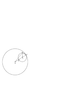
Figure 1: Some geometric relations in the hyperbolic ball model

Using the cosine theorem for the angle $xox^{\prime}$ in the triangle $\Delta_{xox^{\prime}}$ we obtain,

$$\left|x\right|^{2}+1-2\left|x\right|\cos(xox^{\prime})=\left|x-x^{\prime}\right|^{2}\text{ .}$$ (5.11)

Alternatively, by using the triangle $\Delta_{xoc}$ we get

$$\left|x\right|^{2}+\left|w+\frac{1}{2}(1-w)\right|^{2}-2\left|x\right|\left|w+\frac{1}{2}(1-w)\right|\cos(xox^{\prime})=\frac{1}{4}(1-\left|w\right|)^{2}.$$ (5.12)

By eliminating $\cos(xox^{\prime})$ from these two equations we obtain,

$$\frac{1+\left|x\right|^{2}-\left|x-x^{\prime}\right|^{2}}{2}=1+\frac{\left|x\right|^{2}-1}{1+\left|w\right|}\text{ .}$$ (5.13)

This result can be equivalently rewritten as

$$\frac{1-\left|w\right|}{1+\left|w\right|}=\frac{\left|x-x^{\prime}\right|^{2}}{\left|x\right|^{2}-1}\text{ .}$$ (5.14)

The hyperbolic distance $\rho(0,w)$ is known to be $[63]$

$$\rho(0,w)=\ln\left(\frac{1+\left|w\right|}{1-\left|w\right|}\right)\text{ .}$$ (5.15)

Accordingly, the Poisson kernel, Eq.(5.10), can be equivalently rewritten as

$$P_{H}(x,x^{\prime})=\exp\{\alpha\rho(0,w)\}.$$ (5.16)

The hyperbolic Fourier transform can be defined now as $[68]$

$$\varphi_{\alpha}(x)=\frac{1}{\omega_{d}}\int\limits_{S_{\infty}^{d}}d\omega(x^{\prime})\exp\{\alpha<x,x^{\prime}>\}\hat{\varphi}(x^{\prime})$$ (5.17)

with scalar product $<x,x^{\prime}>$ being defined through the hyperbolic distance $\rho(0,w)$ according to Eq.s (5.14),(5.15).

With help of the results just obtained it is possible to give better interpretation of the Ahlfors-Thurston Theorem. Indeed, in view of Eq.s(5.3)-(5.5) we obtain,

$$\varphi(0)=\frac{1}{\omega_{d}}\sum\limits_{\gamma\in\Gamma}\int\limits_{S_{\infty}^{d}}d\omega(x^{\prime})\left(\frac{1-\left|\gamma(0)\right|^{2}}{\left|\gamma(0)-x^{\prime}\right|^{2}}\right)^{d}\chi(x^{\prime}),$$ (5.18)

where ,without loss of generality, we had put x=0 (i.e.placed the initial point x at the center of $B^{d+1})$ .Surely, $\left|\gamma(0)-x\right|^{2}\leq 4$ since we are dealing with the ball of unit radius. Therefore, we also have

$$\varphi(0)<\frac{1}{\omega_{d}}\sum\limits_{\gamma\in\Gamma}\int\limits_{S_{\infty}^{d}}d\omega(x^{\prime})(1-\left|\gamma(0)\right|^{2})^{d}\chi(x^{\prime})\text{ .}$$ (5.19)

Consider now the convergence(or divergence) of the series

$$S_{d}=\sum\limits_{\gamma\in\Gamma}(1-\left|\gamma(0)\right|^{2})^{d}$$ (5.20)

or, more generally,

$$S_{\alpha}=\sum\limits_{\gamma\in\Gamma}(1-\left|\gamma(0)\right|^{2})^{\alpha}\text{ .}$$ (5.21)

Clearly, the last expression is going to be divergent or convergent along with

$$g_{\alpha}(0,0)=\sum\limits_{\gamma\in\Gamma}\left(\frac{1-\left|\gamma(0)\right|}{1+\left|\gamma(0)\right|}\right)^{\alpha}=\sum\limits_{\gamma\in\Gamma}\exp\{-\alpha\rho(0,\gamma(0))\}$$ (5.22)

in view of Eq.s (5.15) and (4.19). But the convergence(divergence) of the Poincar$e^{\prime}$ series , Eq.(5.22), leads us to the results given by Eq.s(5.6)-(5.9). and also earlier stated result, Eq.(4.19).

The results just obtained admit yet another interpretation. Convergence (or divergence) of the series, Eq.(5.22), is associated with existence or nonexistence of the Green’s function acting in $B^{d+1}$as we had mentioned already beforeEq.(5.2). Deep results of Ahlfors$[25]$, Thurston$[42]$, Patterson$[40]$, Beardon$[69]$ and Sullivan $[41]$ state that if the Poincar$e^{\prime}$ series converges, then the Green’s function in $B^{d+1}$ exist and the limit set $\Lambda\subset S_{\infty}^{d}$ is fractal with $areal$ measure equal to zero but $Hausdorff$ dimension equal to $\alpha$ (in this case $\alpha$ lies at the border between the convegence and divergence of the series,Eq.(5.22))and, for d=2, $\alpha\leq 2$ according to Sullivan$[66]$ and Tukia$[67]$ . Additional very important results related to the limit set $\Lambda$ were obtained by Beardon and Maskit$[10]$ who had proved the following

Theorem 5.1.(Beardon Maskit) Let $\Gamma$ be a discrete M$\ddot{o}$bius group of isometries of H³, then, if $\Gamma$ is geometrically finite, the limit set $\Lambda$ comprizes of parabolic limit points and conical limit points .

We would like now to explain the physical significance and the meaning of these statements. First, by looking at Eq.s(4.12)and (4.16) we conclude that $m^{2}\leq 0$ $($because of the results of Sullivan and Tukia). Second, for the group $\Gamma$ to be geometrically finite ($in$ $B^{3})$ it is required that the fundamental domain for $\Gamma$ is being made of finite sided polyhedron $P$ in $B^{3}$ (just like for the Riemann surface of finite genus we should have a finite sided polygon in the unit disk $D$ whose boundary at infinity is $S_{\infty}^{1}).$ Every hyperbolic manifold M³ is defined through use of some fundamental polyhedron $P$ so that, in fact [42],

$$M^{3}=(B^{3}\cup\Omega)/\Gamma$$ (5.23)

where $\Omega=S_{\infty}^{2}-\Lambda$ is the open set of discontinuity of $\Gamma$. In general, $\Omega$ represents some collection of Riemann surfaces which belong to the boundary of $M^{3}.$ This fact has some relevance to problems associated with 2+1 gravity as explained in Ref.[27],[28]. The boundary set $\Omega$ is not accessible dynamically however since it is a $complement$ of the limit set $\Lambda$ in $S_{\infty}^{2}.$ Based in the information provided, study of the hyperbolic 3-manifolds is equivalent to study of the action of discrete subroups $\Gamma$ of the M$\ddot{o}$bius group G on H${}^{3}(or$ B${}^{3})$. In particular, if the quotient, Eq.(5.23), is compact, then $\Gamma$ is said to be cocompact and if the quotient, Eq.(5.23), has finite invariant volume, then $\Gamma$ is said to be cofinite. Incidentally, if $\Gamma$ contains parabolic subgroups, then $\Gamma$ is not cocompact. As it was shown by Thurston$[42]($for some illustrations, please, see also Ref.[70]), complements of most of knots embedded in $S^{3}$are associated with the hyperbolic 3-manifolds. Accordingly, if CFT are to be associated with knots/links (e.g.see Refs[3],[5],[6]), then the corresponding complements of such knots/links, most likely, should be associated with the hyperbolic 3-manifolds. Moreover, the spectral characteristics of different hyperbolic manifolds should be different as well $[19]$. This difference should be also connected with difference in fractal dimensions of the corresponding limit sets which, in turn, will correspond to different type (universality classes)of the CFT. Conversely, given the fractal dimension of the limit set $\Lambda$ , is it possible to determine the Kleinian  (or M$\ddot{o}$bius )group (or groups) which is associated with this limit set ? Evidently, this problem is more complicated than the direct one. Nevertheless, the above discussion is not limited to H³ ( or B${}^{3})$ and, therefore, it becomes potentially possible to study and to classify boundary CFT in dimensions higher than two. More on this subject is presented in sections 7 and 8.

Let us now give the precise definitions of parabolic and conical limit points which were mentioned in the theorem by Beardon and Maskit stated above. An extensive discussion of both parabolic and conical limit points (and sets) could be found in Ref.$[71]$. From this reference we find that ”for any discrete group the set of bounded parabolic points and the set of conical limit points are disjoint”. Given this, and recalling that the parabolic transformations are associated with translations we are left with the following two options(in the case of H${}^{3})$ : a)either the parabolic subgroup has just one generator of translations so that the ”fundamental polyhedron” is the region between two parallel planes as depicted in Fig.2.

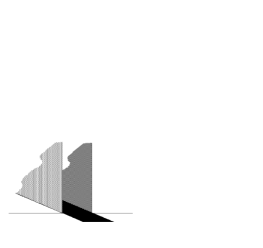
Figure 2: A typical Z-cusp in the upper half space model realization of H³

Such construction is called rank 1 ( or Z- cusp). Evidently,topologically motion $\perp$ to these planes is the same as motion on the circle $S^{1}$ as it was recently discussed at some length in Ref[70]in connection with some problems in polymer physics. Accordingly, such parabolic subgroup is isomorphic to Z or,.b) the parabolic subgroup has two generators so that the ”fundamental polyhedron” is the region defined by the transverse pairs of parallel planes ,as depicted in Fig.3

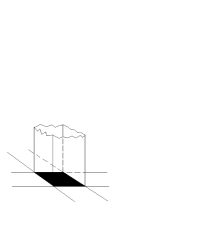
Figure 3: A typical Z$\oplus\mathbf{Z}$ type cusp in the upper half space realization of H³

Such construction is called rank 2 ( or Z$\oplus\mathbf{Z}$ ) cusp. Topologically, motion $\perp$ to such planes is being associated with the motion on the torus. The restriction to have only Z and Z$\oplus\mathbf{Z}$ cusps for hyperbolic 3-manifolds imposes very important restrictions on the boundary CFT to be discussed in section 7.

The conical limit set is not specific to the hyperbolic spaces. According to Ref.[39], in the case of Euclidean half-space H_n for which the typical point y=(x,z), z$>$0, x$\in R^{n-1},$the conical limit set $\Gamma_{\alpha}(a)$ is defined through

$$\Gamma_{\alpha}(a)=\{(\mathbf{x},z)\in H_{n}:\left|x-a\right|<\alpha z\}.$$ (5.24)

Geometrically, $\Gamma_{\alpha}(a)$ is a cone as depicted in Fig.4 with vertex $a$ and axis of symmetry parallel to z-axis.

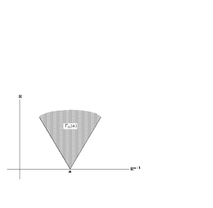
Figure 4: The light cone associated with the conical limit set point located at the boundary of hyperbolic space

A function $u$ defined on H_n is said to have nontangential limit $L$ at $a\in R^{n-1}$ if for every $\alpha>0,u(y)\rightarrow L$ as $y\rightarrow a$ within $\Gamma_{\alpha}(a).$ The term ”nontangential” is being used because no curve in $\Gamma_{\alpha}(a)$ that approaches $a$ can be tangent to $\partial$H${}_{n}=R^{n-1}.$ It is quite remarkable that such nontangential behavior is being observed already for harmonic functions on Euclidean half-space H${}_{n}[39]$ .Use of stereographic projection allows us to formulate the same problem in the Euclidean ball B_n. Respectively, exactly the same definitions are extended to H^d+1 and $B^{d+1}.$Specifically, in the case of $B^{d+1}$ model one can say that $x\in B^{d+1}$ belongs to the cone at $\mathbf{\xi}\in S_{\infty}^{d}$ of opening $\lambda$ and, further, $\left|x-\mathbf{\xi}\right|<2\cos\lambda$ . Analogously to Eq. (5.24), one can write

$$\left|x-\mathbf{\xi}\right|<\alpha(1-\left|x\right|),\text{ }\alpha>0.$$ (5.25)

With such background,we would like discuss in some detail the spectral theory of hyperbolic 3-manifolds. This is accomplished in the next section.

6. Spectral theory of hyperbolic 3-manifolds

In section 3 we had discussed the eigenvalue equation, Eq.(3.7), so that, naively, one might think that this equation provides the complete answer to the question about the spectrum of hyperbolic Laplacian . This is not true, however. Surprisingly, this problem still remains a very active area of research in mathematics. For a comprehensive and very up to date introduction to this field, please, consult Ref[28]. The fact that the spectral theory of hyperbolic Laplacians is absolutely essential for understanding of the spectrum of Hausdorff dimensions of the limit set $\Lambda$ was realized already by Patterson[72] long time ago. Since, even now, the spectrum issue is not completely settled, we would like only to give an outline of the current situation leaving most of the details for future work.

In his 1987 paper$[70]$ Sullivan had stated the Theorem (2.17)(numeration taken from his work)which he calls the Patterson-Elstrodt theorem( incidentally, the recent monograph, Ref[28], is written by Elstrodt ). Based on the results of previous sections it can be formulated as follows:

Theorem 6.1.(Patterson-Elstrodt-Sullivan).

Let

$$-\Delta_{h}\varphi=\lambda\varphi$$ (6.1)

be the eigenvalue problem for the hyperbolic Laplacian on $M^{d+1}=H^{d+1}/\Gamma$ then, the lowest eigenvalue $\lambda_{0}(M^{d})$ satisfies

$$\lambda_{0}(M^{d+1})=\left\{\begin{array}[c]{c}\frac{d^{2}}{4}\text{ if \quad}\alpha\leq\frac{d}{2}\\ \alpha(\Gamma)(\alpha(\Gamma)-d)\text{ if }\alpha\geq\frac{d}{2}\end{array}\right.$$ (6.2)

where $\alpha(\Gamma)$ is the ”critical” exponent of the Poincar$e^{\prime}$ series, Eq.(4.19) or Eq.(5.22).

By looking at Eqs.(4.11),(4.12), these results can be restated as

$$m^{2}=\left\{\begin{array}[c]{c}\lambda_{0}\text{ if }\alpha\geq\frac{d}{2}\\ -\frac{d^{2}}{4}\text{ if }\alpha\leq\frac{d}{2}\text{ .}\end{array}\right.$$ (6.3)

Additional work by Patterson$[62]$ indicates that, at least for $M^{3}$, $0<\alpha\leq 2.$ In view of this , by looking at Eq. (4.12), it is reasonable to consider both ”+” and ”-” branches of solution for $\alpha$ , provided that $-\frac{d^{2}}{4}<m^{2}\leq 0.$ This possibility, indeed, had been recognized in Ref.[75]. The results obtained by Lax and Phillips$[76]$ (and also by Epstein$[77])$ indicate that for 3-manifolds without parabolic cusps the spectrum of -$\Delta_{h}$ acting on $L(M^{3})$ normed metric Hilbert space is of the form:

$$\{\lambda_{0},...,\lambda_{k}\}\cup[\frac{d^{2}}{4},\infty)$$ (6.4)

where

$$0<\alpha(d-\alpha)=\lambda_{0}<\lambda_{1}<...<\lambda_{k}<\frac{d^{2}}{4}$$ (6.5)

are eigenvalues of finite multiplicity and $\lambda_{0}$ has multiplicity one. Moreover, the part of spectrum $[\frac{d^{2}}{4},\infty)$ is absolutely continuous (i.e.for $m^{2}\leq-\frac{d^{2}}{4}$ the spectrum is continuous). The problem with Lax-Phillips$[76]$ and Epstein$[77]$ works lies, however, in the fact that the explicit form of the discrete spectrum had not been obtained. Only the existence of such possibility had been proven.

Remark 6.2. In view of Beardon-Maskit Theorem (section 5) one cannot by pass careful study of the spectrum of hyperbolic Laplacian for some discrete subgroups $\Gamma$ of M$\ddot{o}$bius group G if one is interested in finding the correct fractal dimension of the limit set $\Lambda$ .

For the sake of applications to statistical mechanics (e.g.see section 7) one is also interested in spectral properties of 3-manifolds with parabolic cusps. This can be intuitively understood already now based on the following arguments. If we would choose the sign ”-” in Eq. (4.12) (which,by the way would produce ”+” sign in front of Eq. (4.16), then for $m^{2}$ in the range $-\frac{d^{2}}{4}\leq m^{2}<0$ we would have $\alpha$ in the range $0<\alpha\leq 1$ for d=2. This range is of interest since it covers all physically interesting CFT discussed in the literature$[9].$ If $\alpha$ is to be associated with the Hausdorff dimension of the limit set $\Lambda$, then according to Sullivan ,e.g.see Theorem 2 of Ref.[66], only 3 manifolds with no cusps or rank 1 (Fig.2) cusps will yield $\alpha$ in the desired range. The spectral theory of hyperbolic manifolds with cusps is still under active development in mathematics[29]. Therefore, we would like to restrict ourself with some qualitative estimates of the spectrum based on topological arguments. Here and below we shall discuss only the case d=2 (i.e.H³ or B${}^{3})$. This restriction is by no means severe. It is motivated only by the fact that more explicit analytical results are available for this case in mathematical literature. This, however, does not imply that the case d=2 is more special than say d=3. For instance, Burger and Canary $[78]$ had demonstrated that for any d$>$1 the Hausdorff dimension $\alpha$ is bounded by

$$\alpha\leq(d-1)-\frac{K_{d}}{(d-1)vol(C(M^{d}))^{2}}$$ (6.6)

where $K_{d}$ and $C(M^{d})$ are some d-dependent constants which can be calculated in principle .

In the case if hyperbolic manifold $M^{3}$ is topologically tame (that is it is homeomorphic to the interior of a compact 3 manifold), then Theorem 2.1. of Canary et all $[79]$ states that

Theorem 6.3.(Canary, Minsky and Taylor) If M³ is topologically tame hyperbolic 3-manifold, then the lowest eigenvalue $\lambda_{0}$ of the hyperbolic Laplacian (-$\Delta_{h})$ is given by $\lambda_{0}=\alpha(2-\alpha)$ unless $\alpha<1,$ in which case $\lambda_{0}(M^{3})=1.$

Remark 6.4 As before, $\alpha$ is the Hausdorff dimension of the limit set $\Lambda.$

Remark 6.5 From the above Theorem 6.3. it appears that the results of section 4 become invalid when $\alpha<1$ since Eq.(4.12) cannot be used. The situation can be easily repaired as it is explained in the next section.

Remark 6.6. Theorem 6.3.allows us to obtain the following additional estimates based on recent results by Bishop and Jones$[43].$

Theorem 6.7.(Bishop and Jones). Let $\Gamma$ be any discrete M$\ddot{o}$bius group and let $M^{3}=(B^{3}\cup\Omega)/\Gamma$ . Suppose that the lowest eigenvalue $\lambda_{0}$ is nonzero.Then, there are  constants $C<\infty$ and $c>0$ (depending upon $\lambda_{0}$ only)so that for any x,y with $\rho(\mathbf{x},\mathbf{y})\geq 8$ we have

$$G(\mathbf{x},\mathbf{y})=\int\limits_{0}^{\infty}dtG(\mathbf{x},\mathbf{y};t)\leq\frac{C}{\lambda_{0}}\exp\{-c\rho(\mathbf{x},\mathbf{y})\}$$ (6.7)

where $\rho(\mathbf{x},\mathbf{y})$ is the hyperbolic distance between x and y and $c$=$\min\{\frac{1}{8}\lambda_{0},\frac{1}{4}\}.$

Corollary.6.8.Using this result in combination with Eqs.(4.18),(4.19) and the Theorem 6.3. we obtain, $\alpha=\frac{\lambda_{0}}{8}=\frac{1}{8}.$ If this result is substituted into Eq.(4.16) we obtain the exact result for two-point correlation function of two dimensional Ising model.

Remark 6.9.The theorem of Bishop and Jones depends crucially on the explicit form for the heat kernel $G(\mathbf{x},\mathbf{y};t)$ in H³. Quite recently, Grigori’yan and Noguchi$[80]$ had obtained explicit formulas for the heat kernel for any dimension of hyperbolic space. This opens a possibility to obtain an analogue of inequality (6.7) in any dimension following ideas of Bishop and Jones.

With all plausibility of the Corollary 6.8. it remains to demonstrate that such substitution of $\alpha$ into Eq. (4.16) is indeed legitimate.To this purpose we would like to provide a somewhat different interpretation of Eq.(4.16) in order to demonstrate that Eq.(4.17) makes sense even without arguments associated with Plateau/Dirichlet problem. To begin, we would like, by analogy with the Liouville theorem in standard textbooks on statistical mechanics, to construct a measure associated with the geodesic flow in hyperbolic space.

Following Ref.[25] ,we would like to associate with each point $x\in B^{d+1}\equiv B$ a unit vector $\mathbf{\xi}\in S^{d}$of directions. This vector plays the same role as velocity $\mathbf{v}$ in conventional statistical mechanics. Indeed,$\forall\mathbf{v\neq 0}$ one can construct a vector $\mathbf{\xi}$=$\frac{\mathbf{v}}{\left|\mathbf{v}\right|}$ and then proceed with standard development. The M$\ddot{o}$bius group $\Gamma$ is acting on the phase space T(B)=B$\times S$ according to the rule

$$\left(x,\xi\right)\rightarrow\left(\gamma x,\frac{\gamma^{{}^{\prime}}(x)}{\left|\gamma^{{}^{\prime}}(x)\right|}\xi\right),\text{ }\forall\gamma\in\Gamma.$$ (6.8)

The invariant phase space volume element $d\Omega$ is given therefore by

$$d\Omega=dx_{h}d\omega(\xi)$$ (6.9)

with $d\omega(\xi)$ being a spatial angle measure and dx_h being an element of a hyperbolic volume. The above chosen variables may not be the most convenient ones. More convenient are variables associated with actual location of the ends of geodesics $u$ and $v$ on $S_{\infty}^{d}.$This situation is depicted in Fig.5

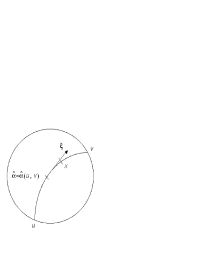
Figure 5: Geometry of geodesics in the ball model of hyperbolic space

It is clear, that $\forall x\in B$ one can select a geodesic which passes through $x$. To this purpose it is not sufficient to assign $u$ and $v$ on $S_{\infty}^{d}$ but, in addition, one has to provide a location $\hat{\alpha}(u,v)$ of the midpoint for such geodesics. Let $s$ be the directional hyperbolic distance between $\hat{\alpha}$ and $x$, then, one should be able to find a correspondence between ($x$,$\xi)$ and $(u,v,s),$ that is one should be able to find a diffeomorphism between $B\times S$ and $S\times S\times R,$ i.e.one expects to find an explicit form of the function $f(u,v)$ which enters into the expression for the volume element given below:

$$d\Omega=dx_{h}d\omega(\xi)=f(u,v)d\omega(v)d\omega(u)ds$$ (6.10)

A simple argument given in Ref[25] produces

$$f(u,v)=\frac{G}{\left|u-v\right|^{2d}}$$ (6.11)

with $G$ being some normalization constant. Looking now at Eq. (3.22), it is clear, that one can now replace it with

$$\hat{D}[\varphi]=\int\frac{d\Omega}{ds}\varphi_{0}(u)\varphi_{0}(v)\text{ .}$$ (6.12)

It is also clear, in view of the transformation properties of the function $\varphi_{0}$given by Eq.(4.14), that, in general, one can replace Eq.(6.12) with

$$\hat{D}[\varphi]=G\int\frac{\varphi_{0}(u)\varphi_{0}(v)}{\left|u-v\right|^{2\alpha}}d\omega(v)d\omega(u)$$ (6.13)

where the exponent $\alpha$ is associated with the Hausdorff dimension of the limit set $\Lambda$ .This is indeed the case, e.g.see page 286 of Ref[64]. Thus, the exponent $\alpha$ in Eq. (6.13) is the same as the exponent $\alpha$ in Eq. (5.22). This observation provides the necessary support to the claims made after Eq.(6.7).

Given all above, the obtained results show no apparent connections with the existing conformal field theories. We would like to correct this deficiency in the next two sections.

7. Connections with the existing formalism of CFT

In section 5 we had introduced Z and Z$\oplus\mathbf{Z}$ cusps, e.g. see Figs 2,3. According to Sullivan$[66],$only 3-manifolds with no cusps or just Z-cusps will produce limit sets $\Lambda$ with Hausdorff dimension $\alpha$ in the range $0<\alpha\leq 1.$ Naively, it means, that only consideration of the CFT on the strip with periodic boundary conditions(thus making it a cylinder) will yield the critical exponents for two point correlation functions in the above range. This case is, indeed, frequently discussed in physics literature$[9].$ For the strip of width L use of the conformal transformation

$$z^{\prime}=w(z)=\frac{L}{2\pi}\ln z$$ (7.1)

converting strip of width $L$ to the entire complex plane (rigorously speaking, we are dealing here with $\mathbf{C\backslash\{0\}}$ complex plane$[81]$). Although the above discussion appears to be plausible ,the description of Z-cusps (as well as Z$\oplus\mathbf{Z}$ cusps ) is actually considerably more sophisticated. In this paper we only provide a brief outline of what is actually involved reserving full treatment for future publications.

In section 5 we had noticed that $\Lambda$ may contain no more than two limiting points (elementary set) or infinite number of points (non-elementary set). The Kleinian groups which are associated with the elementary limit sets are known $[8],[31]$ and, basically, are reducible to the following list:

1) a parabolic infinite cyclic Abelian group $\Gamma:$ $z\rightarrow z+1;$

2) a parabolic rank 2 Abelian group $\Gamma$ : $z\rightarrow z+1,z\rightarrow z+\tau$ ; $\operatorname{Im}\tau>0;$

3) a loxodromic cyclic group $\Gamma$ : z$\rightarrow\lambda z$ with $\lambda\in\mathbf{C}\backslash\{0,1\}.$

Let now $M^{3}$ be some 3-manifold and let $M_{(0,\varepsilon)}$ be a subset of points $p\in M^{3}$ such that there is a closed nontrivial curve passing through $p$ whose hyperbolic length $l$ is less than $\varepsilon$. Then, if $\varepsilon<2r_{0}$ where $r_{0}$ is some known (Margulis)constant, the $M_{(0,\varepsilon)}$ part of $M^{3}$ (the ”thin part”) is a quotient $H^{3}/\Gamma$ where $\Gamma$ is just one of these three elementary groups. The complement of $M_{(0,\varepsilon)}$ in $M^{3}$ is called ”thick” part. The above construction is not limited to $M^{3}$and is applicable to $\mathbf{any}$ $M^{d+1}($with Margulis constant being, of course, different for different d’s). The ”thin” part is associated with Z and Z$\oplus\mathbf{Z}$ cusps.

Remark 7.1.Recently, we had briefly considered the ”thick ” -”thin” decomposition of hyperbolic 3-manifolds in connection with dynamics of 2+1 gravity $[36],[37].$ For a comprehensive mathematical treatment of these issues, please, consult Ref[42],[71],[82].

To realize, that the ”thin” part is associated with Z cusps it is sufficient to look at H² model of hyperbolic space first. In this case, the following Theorem can be proven$[83]$

Theorem 7.2. Let G be Fuchsian group operating on H² .If G contains a parabolic element, then H${}^{2}/G$ contains a puncture.The number of punctures is in one-to-one correspondence with the number of conjugacy classes of parabolic elements.

Recall now, that in 3 dimensional case $\Omega=S_{\infty}^{2}-\Lambda$ and, using Eq.(5.27), it is possible to show that $\Omega/\Gamma$ is just a collection of Riemann surfaces $[44]$ . In the case if we are dealing with Z-cusps these surfaces will contain punctures as it was first noticed by Ahlfors$[84]$. The number of cusps (=punctures) N_c is related to the number of generators N of the Kleinian group acting on H${}^{3}.$ According to Sullivan$[85]$(and also Abikoff$[86])$

$$\text{N}_{c}\leq 3\text{N-4}$$ (7.2)

In the language of the CFT the punctures are usually associated with the vertex operators$[9].$ The presence of punctures converts Riemann surface $R$=$\Omega/\Gamma$ into the marked Riemann surface$[27].$ We shall, for simplicity, treat the quotient $\Omega/\Gamma$ as just one Riemann surface (unless the otherwise is specified) keeping in mind that there could be finitely many(Ahlfors finiteness theorem$[84])$. Among marked surfaces one can choose some reference Riemann surface X for which the marking is fixed. Then, other surfaces could be related to X via homeomorphism f: $R\rightarrow$X sending the orientation on R into orientation on X. The Teichmüller space, Teich($R$), associates conformal structures on R in which each boundary component corresponds to a puncture. Two marked surfaces (f${}_{1,}R_{1})$ and (f${}_{2},R_{2})$ define the same point in Teichmüller space Teich(R) if there is a complex analytic isomorphism i: $R_{1}\rightarrow R_{2}$ such that i$\circ$f₁ is homotopic to f${}_{2}.$ Two surfaces $R_{1}$ and $R_{2}$ belong to two different points in Teichmuller space if the Teichmüller metric (distance)

$$d(R_{1},R_{2})=\frac{1}{2}\inf\ln K(\phi)$$ (7.3)

is greater than zero. Here $\phi:$ $R_{1}\rightarrow R_{2}$ ranges over all quasiconformal maps in the homotopy class f${}_{2}\circ$f${}_{1}^{-1}($relative to the punctures) so that K($\phi)$ is maximum dilatation of $\phi.$ The above formula is not immediately useful since we have not defined yet what is meant by dilatation.To correct this deficiency, let us consider the Beltrami coefficient (for suggestive physical interpretation, please, consult Ref[37])

$$\mu_{f}=\frac{\partial_{\bar{z}}f(z)}{\partial_{z}f(z)}$$ (7.4)

For functions f₁and f₂ introduced above we obtain respectively $\mu_{1}$ and $\mu_{2}.$Then,the maximum dilatation can be defined as

$$K(\phi)=\frac{1+r}{1-r}\text{ \quad where }r\text{=}\left\|\frac{\mu_{1}-\mu_{2}}{1-\bar{\mu}_{1}\mu_{2}}\right\|_{\infty}$$ (7.5)

according to [30],[44], with $\left\|\cdot\cdot\cdot\right\|_{\infty}$ being determined by the requirement $[44]$

$$\left\|\mu_{f}(z)\right\|=\sup_{z\in R}\left|\mu_{f}(z)\right|<1.$$ (7.6)

From the above results it follows, that if $\gamma\in\Gamma$ and z$\in S_{\infty}^{2},$ then

$$\mu(\gamma(z))\frac{\bar{\gamma}^{\prime}(z)}{\gamma(z)}=\mu(z)\text{ \quad}\forall z\in\Omega$$ (7.7)

and

$$\mu(z)=0\text{ \quad}\forall z\in\Lambda.$$ (7.8)

Let us now fix $\mu$ and introduce f${}^{\mu}(z)$ instead (that is f${}^{\mu}(z)$ is some function which produces the Beltrami coefficient according to Eq.(7.4)). The mapping $\Gamma\rightarrow\Gamma^{\mu}$ given by $\gamma\rightarrow$f${}^{\mu}\circ\gamma\circ($f${}^{\mu})^{-1}$ is called quasiconformal (or $\mu-conformal)$ deformation. Let us notice now that normally the Riemann surface $R$ is being defined as quotient $R$=H${}^{2}/G$ where G is some discrete Fuchsian group. In the case of $S_{\infty\text{ }}^{2}$we have a rather peculiar situation: Kleinian group $\Gamma\subset PSL_{2}(C)$ plays the same role as Fuchsian G$\subset PSL_{2}(R).$ One can bring these two together by noticing that H² model corresponds to an open disc D. Then, one can glue two copies of D together thus forming $S_{\infty\text{ }}^{2}.$ Kleinian group $\Gamma$ acting on $S_{\infty}^{2}$ can be considered as Fuchsian on each of these two disks. The mapping $\Gamma\rightarrow\Gamma^{\mu}$ may affect the gluing boundary between the two disks. If we use f^μ to produce ”new” group from the ”old”, i.e.,

$$\gamma^{\mu}=f^{\mu}\circ\hat{\gamma}\circ(f^{\mu})^{-1},$$ (7.9)

then thus obtained new group is called quasi-Fuchsian (provided that $\hat{\gamma}$ is Fuchsian) if the gluing boundary between two disks is still topologically a circle $S^{1}(e.g.$ see Thurston’s lecture notes$[42]$, section 8.34). This gluing boundary may include $\Lambda$ as a part only or, it could be that $\Lambda=S^{1}.$

Recently, Canary and Taylor $[46]$ had proved the following remarkable theorem.

Theorem 7.3.(Canary and Taylor). Let $\Gamma$ be a nonelementary finitely generated Kleinian group and let $\Lambda$ denote its limit set. If the Hausdorff dimension $\alpha$ of $\Lambda$ is less than one, then $\Gamma$ is geometrically finite and has a finite index subgroup which is quasiconformally conjugate to a Fuchsian group of the second kind .

Remark 7.4. Recall$[87]$, that for the Fuchsian groups of the second kind the limit points are nowhere dense on $S^{1}.$Since, according to results of section 6, we are interested mainly in the $\alpha-$domain given by $0<\alpha\leq 1,$ we notice that we have to deal with the quasiconformal deformations of $S^{1}$ associated with Fuchsian groups of the second kind.

For completeness, we would like also to provide the results related mainly to the Fuchsian groups of the first kind for which the limit set $\Lambda$ coincides with $S.$ These are summarized in the following

Theorem 7.5.(Canary and Taylor$[46])$ Let $\Gamma$ be a nonelementary finitely generated Kleinian group and let $\Lambda$ denote its limit set. If $\alpha=1$, then $\Gamma$ either a function group with connected domain of discontinuity or contains a subgroup of index at most 2 which is the Fucsian group of the first kind. Alternatively, if  $\alpha=1$ and $\Gamma$ is geometrically finite, then either $\Gamma$ has a finite index subgroup which is quasiconformally conjugate to a Fuchsian  group of the second  kind or $\Gamma$ contains a subgroup of index at most 2 which is the Fuchsian group of the first kind.

Remark 7.6.Much earlier Bowen$[88]$ had proven an analogous theorem for the Fuchsian groups of the first kind. According to Bowen, the Hausdorff dimension of $\Lambda$ is greater than one. Since Bowen’s proof is nonconstructive, there is no way to estimate, based on his results, to what extent $\alpha$ is larger than one. Thus, there is no contradiction between Theorem 7.5. and Bowen’s results since $\alpha$ can be infinitesimally close to 1.

Remark 7.7.For the case of Fuchsian groups of the first kind it is known $[88],$ that $\Omega/\Gamma$ consists of exactly two Riemann surfaces :one for each disk D. It is also known$[45],$ that for the Fuchsian group of the second kind $\Omega/\Gamma$ is made of just one Riemann surface so that $S_{\infty}^{2}$ is boundary at infinity for this surface.

In mathematics literature$[31]$ a finitely generated non elementary Kleinian group which has just one invariant component $\Omega$ is called function group. If, in addition, $\Omega$ is simply connected, then such group is called B-group. More complicated Kleinian groups could be constructed from simpler ones and B-group is one of the main building blocks in such construction[90].

Remark 7.8.In string theory (and, therefore, in the CFT)the Schottky-type groups are being used$[91]$. Schottky group is a function group but not a B-group [31].

Remark 7.9. There is one-to one correspondence between the quasiconformal deformations of Kleinian groups and quasisometric deformations of hyperbolic 3-manifolds. The theory is not limited to 3-manifolds, however, and can be considered for any d$\geq 2.$ More specifically, there is a

Theorem 7.10. For a quasiconformal automorphism f of $S_{\infty}^{2}$ compatible with a Kleinian group $\Gamma$, there exist a quasi-isometric automorphism F of H³ which is an extension of f and which is compatible with $\Gamma$, namely, F$\circ\gamma\circ$F$\in Mob(B^{3})$ for any $\gamma\in\Gamma.$

Proof: Please, consult Ref.[31] (page 157).$\square$

Remark 7.11.The above theorem follows directly from the discussion related to Eq.s (7.7)–(7.9) and for additional details and motivations, please, consult the work by Bers, Ref.[45].

Remark 7.12.The above Theorem is applicable to the case when, instead of $S_{\infty}^{2},$ we use $S_{\infty}^{1}($taking into account the results on Canary and Taylor, Theorems 7.3 and 7.5)

The observations presented above allow us to make a direct connection with the existing results associated with 2 dimensional CFT. To begin, let us notice that if we would have $S_{\infty}^{1}$ as limit set $\Lambda$ for the Fuchsian groups of the first kind, then, according to Eq. (7.8) we could not use the quasiconformal mapping and, accordingly,we would be stuck with just one conformal structure. This fact is known in mathematics as Mostow rigidity theorem. Usually, this theorem is applied to spaces of dimensionality $\geq 3$ (for more details,please,see section 8).At the same time, if we consider Fuchsian groups of the second kind, then, we need to deal with maps of $S_{\infty}^{1}$ acting on some open intervals (since $\Lambda$ is closed set) of $S_{\infty}^{1}.$ This is not exactly the situation which is known in physics literature. Indeed, in physics literature on CFT one is dealing with the Virasoro algebra. Let us recall how one can arrive at this algebra. Following Ref.[56], let us consider the group G=$DiffS^{1}$ of orientation preserving diffeomorphisms of $S_{\infty}^{1}.$ Let $\alpha_{1}(z)$ and $\alpha_{2}(z)$ be two elements of G, then the group composition law can be defined by

$$\alpha_{1}\circ\alpha_{2}(z)=\alpha_{1}(\alpha_{2}(z))\text{ \quad, }z=\exp\{i\theta\}.$$ (7.10)

The representation of the group G is defined according to the following prescription:

$$U(\alpha)f(z)=f(\alpha^{-1}(z)),$$ (7.11)

where the operator $U(\alpha)$ acts on the vector space of smooth complex-valued functions on $S_{\infty}^{1}.$The explicit form of the operator $U(\alpha)$ can be easily found if one notices that

$$\alpha(z)=z(1+\varepsilon(z))=z+\sum\limits_{n=-\infty}^{\infty}\varepsilon_{n}z^{n+1},\text{ }\varepsilon_{n}\rightarrow 0^{+}.$$ (7.12)

Using this expansion and keeping only terms up to 1st order in $\varepsilon_{n}$ we obtain,

$$U(\alpha)f(z)=f(z-\sum\limits_{n=-\infty}^{\infty}\varepsilon_{n}z^{n+1})=(1+\sum_{n}\varepsilon_{n}\hat{d}_{n})f(z)$$ (7.13)

with operator $\hat{d}_{n}$ given by

$$\hat{d}_{n}=-z^{n+1}\frac{d}{dz}=i\exp\{in\theta\}\frac{d}{d\theta}.$$ (7.14)

The operators $\hat{d}_{n}$ form a closed Lie algebra $VectS^{1}$ described in terms of the following commutator

$$\left[\hat{d}_{m},\hat{d}_{n}\right]=(m-n)\hat{d}_{m-n}$$ (7.15)

The central extension of this algebra (to be discussed later in this section) produces the Virasoro algebra. $VectS^{1}$ contains a closed subalgebra formed by $\hat{d}_{0},\hat{d}_{1}$ and $\hat{d}_{-1}$ corresponding to the infinitesimal conformal transformations of the extended complex plane $S^{2}$=$\mathbf{C\cup\{\infty\}}$ caused by the action of PSL$(2,C).$ Thus, even though we had started with diffeomorphisms of the circle, we ended up with the automorphisms of the extended complex plane. The question arises: is such extension unique ? The answer is: ”no” ! Because of this negative answer, there is a real possibility of extension of the operator formalism of 2d CFT to higher dimensions. This issue is going to be discussed in the next section. For the time being,we would like to explain the reasons why the answer is ”no”.

Following Ahlfors$[92]$, and, more recently, Gardiner and Sullivan$[93],$we would like to consider a quasisymmetric mapping (to be defined below) of the disk D to itself which induces a topological mapping of the circumference, i.e. S${}_{\infty}^{1}.$ To this purpose it is convenient to use a conformal transformation which converts the disk model to the upper halfplane Poincar$e^{\prime}$ model of the hyperbolic space H${}^{2}.$ Next, it is convenient to select points x,x-t, and x+t on the real line R (corresponding to $S_{\infty}^{1})$ so that the mapping $h(x)$ satisfies the M-condition

$$M^{-1}\leq\frac{h(x+t)-h(t)}{h(x)-h(x-t)}\leq M$$ (7.16)

Let $h$ be a homeomorphism mapping of an open intrerval I of the real axis into the real axis. Then, $h$ is quasisymmetric on I if there exist a constant M such that the inequality (7.16) is satisfied for all x-t, x, x+t in I. Thus defined quasisymmetric mapping forms a group(which we shall denote as QS) which obeys the same composition law as given by Eq.(7.10) (except now z is on the real line). The real line $\mathbf{R}$ is the universal covering of the circle. The exponential mapping, exp (2$\pi i\theta),$ induces an isomorphism between R/Z and $S^{1}.$ The homeomorphism h(x) of $S^{1}$which is characterized by the properties $[93]$

$$h(0)=0,\text{ }h(x)+1=h(x+1)$$

can be lifted to a homeomorphism $\tilde{h}(x)$ of $\mathbf{R}$ which obeys the following inequalities:

$$1-\varepsilon(t)\leq\frac{\tilde{h}(x+t)-\tilde{h}(x)}{\tilde{h}(x)-\tilde{h}(x-t)}\leq 1+\varepsilon(t),$$ (7.17)

where $\varepsilon$ converges to zero with t.

It is easy to check that this result is consistent with Eq.(7.12) and, therefore, the group G=$DiffS^{1}$ is called the group of symmetric homeomorphisms. G is proper subgroup of QS$[93].$ Looking at Eq.(7.5) and identifying $r$ with $\varepsilon(t)$ we conclude, that the subgroup G has boundary dilatation asymptotically equal to one. That is such transformation do not cause the deformations of hyperbolic 3-manifolds. The above deficiency of the group G was recognized and corrected in the fundamental work by Nag and Verjovsky $[48].$ Below, we would like to provide the summary of their accomplishments in the light of results just described and with purpose of extension of these results in section 8. In order to do so, we still need to make several observations related to QS group. Let us begin with

Theorem 7.13.(Ahlfors-Beurling$[94])$ Assume $h$ is homeomorphism of R .Then, h is quasisymmetric if, and only if, there exists a quasiconformal extension $\tilde{h}$ of $h$ to the complex plane . If $h$ is normalized to fix three points, say 0,1 and $\infty,$ then $h$ is quasisymmetric with constant M. The quasiconformal extension $\tilde{h}$ can be selected so that its dilatation $K$ is less than or equal to $c_{1}(M)$ where $c_{1}(M)\rightarrow 1$ as $M\rightarrow 1.$

Remark 7.14. The symmetric homeomorphism $\alpha(z)$ by contrast fixes only one point: z=0. Some explicit examples of construction of $\tilde{h}$ are given in the papes by Carleson$[95]$ and Agard and Kelingos [96].

Remark 7.15.Because $c_{1}(M)\rightarrow 1$ when M$\rightarrow 1$ any symmetric homeomorphism of S¹ can be approximated by quasisymmetric one. This is the most important fact facilitating development of conformal field theories beyond 2 dimensions.

Remark 7.16. Construction of $h$ is closely related to study of maps of the circle as it is known in the theory of dynamical systems$[97]$. Evidently,one is interested in maps which map points $\in\Lambda$ to points in $\Lambda$ and (or), alternatively, in maps which map points in $\Omega$ to points in $\Omega.$ Notice, that under such conditions the Lie algebra $VectS^{1}$can always be constructed since its construction requires only existence of some open interval around any point z$\in\Omega.$ But, by definition, the set $\Omega$ is open.

Let us discuss now the issue of central extension of $VectS^{1}.$ The need to introduce the central extension of the Lie algebra $VectS^{1}$ is by no means intrinsic just for this group. Already Schur developed general method of constructing projective representations of finite groups about a hundred years ago. The extension of his method to Lie groups is relatively straightforward and is wonderfully presented in the book by Hamermesh$[98]$. The comprehensive up to date summary of results in this direction could be found in the encyclopedic work, Ref[99]. It is not our purpose to provide a review of these results. We would like here to explain the physical motivations leading to the projective representations of Lie groups since the central extension is directly related to construction of these projective representations.

As is well known, there are actually two different ways to solve quantum mechanical problems. The first one comes from mathematics of solving of 2nd order ordinary differential equations while the second one comes from the algebraic (group-theoretic) approach to the same problem. The projective representations are naturally associated with the second approach. In particular, let g₁ and g₂ be two elements of some Lie group G. One can think of unitary representations associated with group G. That is one can try to find a unitary operator $U(g)$, $g\in G,$ such that

$$U(g_{1})U(g_{2})=U(g_{1}\circ g_{2})\text{ .}$$ (7.18)

Such representation of the group G is called vector representation(by analogy with finite dimensional space where the role of $U$ is being played by finite matrices acting on vectors). In quantum mechanics, as is well known, the wave function is determined with accuracy up to a phase factor. This means that, along with Eq.(7.18), one can think of alternative way of writing the composition law, e.g.

$$U(g_{1})U(g_{2})=\omega(g_{1},g_{2})U(g_{1}\circ g_{2})\text{ .}$$ (7.19)

Surely, one should require $\left|\omega(g_{1},g_{2})\right|=1.$ This then allows us to write the factor $\omega(g_{1},g_{2})$ as

$$\omega(g_{1},g_{2})=\exp\{i\xi(g_{1},g_{2})\}$$ (7.20)

The phase factor $\xi(g_{1},g_{2})$ is associated with the topology of the underlying group space. Finally, in our case of $DiffS^{1}$ the action of the operator $U(g)$ on the vector $f(z)$ is given by Eq.s(7.11)-(7.13) so that the composition law, Eq.(7.19), along with definition, Eq.(7.20), allows us to obtain in a rather standard way$[100]$ the centrally extended Lie algebra $VectS^{1}$ which is known as Virasoro algebra and it is given by

$$\left[\hat{d}_{m},\hat{d}_{n}\right]=(m-n)\hat{d}_{m-n}+\hat{c}a(m,n)$$ (7.21)

where $\hat{c}$ is some number (related to the central charge) and the two-cocycle $a(m,n)$ is related to $\xi(g_{1},g_{2})$ and can be easily obtained explicitly by using the Jacoby identity and the commutation relations given by Eq.(7.21). The final result can be written in the form suggested by Kac$[56]$

$$\left[\hat{d}_{m},\hat{d}_{n}\right]=(m-n)\hat{d}_{m-n}+\delta_{m,n}\frac{(m^{3}-n)}{12}c$$ (7.22)

with c being the central charge. For the developments presented below in this paper it is very important to recognize the physical reason for the emergence of the two-cocycle a(m,n). Nag and Verjovsky$[48]$ had demonstrated that it is related to the quasisymmetric deformations of the projective structures on $S^{1}$by diffeomorphisms. These structures were fully classified in Ref[101]. Basically, they are associated with group of M$\ddot{o}$bius transformatoions PSL(2,R)

$$x=\frac{ax+b}{cx+d}$$ (7.23)

on the real line. Study of the deformations of the projective structure on the line which was initiated by Ahlfors and Beurling$[94]$ was considerably developed by Carleson$[95]$ and Agard and Kelingos$[96]$ and culminated in the work of Nag and Verjovsky$[48]$ . To make our presentation self-contained, we would like now to summarize their results from the point of view of ideas presented in this section. This summary is needed whenever one is contemplating about the extension of the existing 2 dimensional results related to CFT to higher dimensions (to be discussed in some detail in the next section).

Consider a quotient T(1)=QS/PSL(2,R) that is the space of ”true” quasisymmetric deformations which fix 3 points, e.g.say, 1,-1 and -i on $S^{1}$, then T(1) is associated with universal Teichmüller space in a sense of Bers$[102].$ The space $M=DiffS^{1}/PSL(2,R)$ is embeddable inside of T(1). The space $M$ can be equipped with the complex structure so that it becomes infinite dimensional Kähler manifold. For the vectors $v=\sum\limits_{m}v_{m}\hat{d}_{m}$ and $w=\sum\limits_{m}w_{m}\hat{d}_{m}$ tangent to $M$ at some point chosen as the origin one can construct the Kähler metric g($v,w).$ The most spectacular result of Ref [48] lies in the proof of the fact that the Kähler 2-form

$$\omega(v,w)=g(v,\tilde{J}w),$$ (7.24)

where $\omega(v,w)=\sum\limits_{n,m}v_{n}w_{m}a(m,n),$ with $a(m,n)$ being the same as in Eq.(7.21), (7.22), and $\tilde{J}w$ being defined through equation

$$\tilde{J}w=\sum\limits_{m}(-i)sign(m)w_{m}\hat{d}_{m},$$ (7.25)

coincides with the Weil-Petersson metric,

$$g(v,w)=\text{W-P}(v,w)$$ (7.26)

where W-P$(v,w)$ is the Weil-Petersson (W-P) metric on T(1).The Weil-Petersson metric on Teicmüller space is discussed in sufficient detail in Ref[45].If $\mu(z)\frac{d\bar{z}}{dz}$ is the Beltrami differential,e.g. see Eq.(7.4),and $\varphi([\nu])(z)dz^{2}$ is the quadratic differential (e.g. see Ref[37] for an elementary discussion of quadratic differentials) then, the W-P inner product is defined by the following formula

$$<\mu,\varphi[\nu]>=\text{W-P}(\mu,\nu)$$ (7.27)

$$=\text{{}}\iint\limits_{\Delta/F}\times\iint\limits_{\Delta}\frac{\mu(z)\bar{\nu}(\zeta)}{(1-z\bar{\zeta})^{4}}d\xi d\eta dxdy$$

with $\nu\rightarrow\varphi([\nu])(z)$ being given by

$$\varphi([\nu])(z)=\iint\limits_{\Delta}\frac{\bar{\nu}(\zeta)}{(1-z\bar{\zeta})^{4}}d\xi d\eta$$ (7.28)

, here$z=x+iy$ , $\zeta=\xi+i\eta$ and $\Delta$ is the unit disk with F beingsome Fuchsian group thus making the quotient $\Delta/F$ a Riemann surface. In the present case F$\equiv 1$ as it will be explained shortly. In view of this, one should not worry about F.

Remark 7.17.a) The Kalerity of W-P metric expressed by Eq.(7.24) had actually been proven by Ahlfors$[49]$ in 1961. b) In the same paper by Ahlfors, Eq.(7.28) has been derived which differs in sign and numerical prefactor from Eq.(7.28). This, fortunately, plays no role in the final results obtained in Ref.[48].

Remark 7.18 Since Eq.(7.28) plays the central role in the rest of calculations presented below,we would like to provide some additional information related to this equation(not contained in Ref[48]) in order to help physically educated reader to appreciate its significance . To this purpose let $\mu_{f}$ in Eq.(7.4) be written as $\mu(t)(z)=t\nu(z).$ Then, it can be shown [44] that for solution $f^{\mu}$ of the Beltrami Eq.(7.4) the following limiting result holds

$$\dot{v}[\mu](z) =\lim_{t\rightarrow 0}\frac{f^{\mu}-z}{t}$$ (7.29)

$$=-\frac{1}{\pi}\iint\limits_{H^{2}}\nu(z)\frac{z(z-1)}{\zeta(\zeta-1)(\zeta-z)}d\xi d\eta\text{ .}$$

With help of Eq.(7.29) we obtain,

$$f^{\mu}(z)=z+\dot{v}[\mu](z)t+o(t)\text{ , }t\rightarrow 0,$$ (7.30)

to be compared with Eq.(7.12). From this comparison it follows, that the quasisymmetric vector field $\mathbf{v}$ on $S^{1}$ can be defined as

$$v=\dot{v}[\mu](z)\frac{d}{dz}.$$ (7.31)

In addition, using Eq.(7.30), we obtain,

$$\frac{d}{dz}f^{\mu}(z)=1+t\frac{d}{dz}\dot{v}[\mu](z)\equiv 1+t\dot{v}[\mu]^{\prime}$$ (7.32)

and also,

$$\frac{d^{2}}{dz^{2}}f^{\mu}(z)=t\dot{v}[\mu]^{\prime\prime}$$ (7.33)

and

$$\frac{d^{3}}{dz^{3}}f^{\mu}(z)=t\dot{v}[\mu]^{\prime\prime\prime}\text{ .}$$ (7.34)

The Schwarzian derivative of $\{f^{\mu},z\}$ defined by

$$\varphi_{t}[\nu\}(z)=\{f^{\mu},z\}=\frac{f^{\prime\prime\prime}(z)}{f^{\prime}(z)}-\frac{3}{2}\left(\frac{f^{\prime\prime}(z)}{f^{\prime}(z)}\right)^{2}$$ (7.35)

can now be constructed so that in the limit $t\rightarrow 0$ using Eqs(7.32)-(7.35) we obtain,

$$\varphi_{t}[\nu](z)=t\dot{v}[\mu]^{\prime\prime\prime}+o(t)\text{ .}$$ (7.36)

Let now $\mu(t)=\mu+t\nu[z],$ then we can construct

$$\varphi[z](z) =\frac{\varphi_{t}[\nu](z)-\varphi_{0}[\nu](z)}{t}$$ (7.37)

$$=-\frac{12}{\pi}\iint\limits_{H^{2}}\frac{\bar{\nu}(z)}{(\bar{\zeta}-z)^{4}}d\xi d\eta$$

where the use was made of Eq.(7.29) in order to perforn z-differentiation in eq.(7.36) explicitly. Obtained result is documented on p.138 of Ahlfors book, Ref[92], and should be compared against Eq.(7.28) upon conversion from H² plane to the disc $\Delta$. Since it is well known$[44]$ that the Schwarzian derivative acts like a quadratic differential under the transformations which belong to the Fuchsian group F, we conclude that, indeed, up to unimportant constant (which may differ from $-\frac{12}{\pi}$ when the transformation from H² to $\Delta$ is made ) Eqs.(7.28) and (7.37) are equivalent.

Next, by combining Eqs.(7.21),(7.24),(7.25) it can be shown, that

$$g(v,w)=-2i\hat{c}\operatorname{Re}\sum\limits_{m=2}^{\infty}\bar{v}_{m}w_{m}(m^{3}-m).$$ (7.38)

In addition, it is possible to show that the Fourier coefficients of $\dot{v}[\mu]$ (and, analogously, $\dot{w}[\mu])$ defined by Eq.(7.31),are given by

$$v_{k}=\frac{i}{\pi}\iint\limits_{\Delta}\bar{\mu}(z)z^{k-2}dxdy,$$ (7.39a)

and

$$w_{k}=\frac{i}{\pi}\iint\limits_{\Delta}\nu(z)z^{k-2}dxdy\text{ , k}\geq 2.$$ (7.39b)

Using these results in Eq.(7.38), we obtain,

$$\sum\limits_{m=2}^{\infty}\bar{v}_{m}w_{m}(m^{3}-m)=-\frac{1}{\pi^{2}}\iint\limits_{\Delta}\times\iint\limits_{\Delta}\mu(z)\bar{\nu}(\zeta)(\sum\limits_{m=2}^{\infty}z^{m-2}\bar{\zeta}^{m-2}(m^{2}-m))d\xi d\eta dxdy$$ (7.40)

Using summation formula

$$\sum\limits_{m=2}^{\infty}(m^{3}-m)x^{m-2}=\frac{-1}{6(1-x)^{4}}\text{ ,}\left|x\right|<1$$ (7.41)

in Eq(7.40) we obtain,

$$g(v,w)=-\frac{i\hat{c}}{3\pi^{2}}\text{W-P}(\mu,\nu)$$ (7.42)

with W-P$(\mu,\nu)$ being defined by Eq.(7.27) were now we have to put F=1. Surely, $\hat{c}$ can be replaced by $ib$ and we can adjust $b$ in such a way that $\frac{b}{2\pi^{2}}=\frac{c}{12}$ in accord with Eq.(7.22).

Thus, we have demonstrated, following Nag and Verjovsky$[48]$, that the central charge of the Virasoro algebra is directly associated with the quasisymmetric deformations of $\Delta$ (or H${}^{2}).$In view of this fact, it becomes possible to consider extensions of the existing formalism to higher dimensions. This is the subject of the next section.

Remark 7.18. Since the Virasoro algebra, Eq.(7.22), with fixed central charge provides solution of a particular CFT at criticality, to crossover from one universality class (given by fixed central charge) to another (given by different value of the central charge) Zamolodchikov [103] had developed theory (known in physics literature as c-theorem) which describes the dynamics of crossover between different values of central charge. It would be very interesting to explain his results by developing ideas of Nag and Verjovsky[48].

8. Beyond two dimensions

In 1968 Mostow$[104]$ proved very important theorem which is known as Mostow rigidity theorem. It can be formulated as follows.

Theorem 8.1.(Mostow)Let N=H${}^{d+1}/\Gamma$ be a complete hyperbolic manifold , d$\geq 2,$ and let N${}^{{}^{\prime}}=$H${}^{d+1}/\Gamma^{\prime}$ be some other hyperbolic manifold, then if there is a quasi-isometric homeomorphism f: N$\rightarrow$N${}^{{}^{\prime}}$, then f is homotopic to an isometry N$\rightarrow$N^′ if and only if both Möbius groups $\Gamma$ and $\Gamma^{\prime}$ are of the first kind (i.e. $\Omega=S_{\infty}^{d}-\Lambda=0$,e.g. see section 5).

Remark 8.2.This result could be easily understood in view of Eq.s (7.7) and (7.8). For an additional illustration of the existing possibilities one is encouraged to look at the paper by Donaldson and Sullivan$[105]$ who established that some closed four-manifolds have infinitely many distinct quasiconformal structures while others do not admit the quasiconformal structure at all.

Remark 8.3.Mostow rigidity theorem can be viewed as an extension and ramification of much earlier theorem by Liouville (originally proven in 1850)$[106]$ which can be stated as follows.

Theorem 8.4.(Liouville) Let $U$ be some open subset of R${}^{d}\cup\{\infty\}\equiv$R̂^d and let f :$U\rightarrow$R̂^d be a conformal map, then f is just a M$\ddot{o}$bius transformation for d$\geq 3.$

It is because of this theorem, known in physics literature$[9],$ there is a widespread belief that results of two dimensional CFT cannot be extended to higher dimensions.

Remark 8.5. In order to study d dimensional systems at criticality (d$\geq 2)$ one should look for the M$\ddot{o}$bius groups of the second kind . Then, the question arises immediatly : is there an analogue of physically funadamentally important Canary-Taylor theorems (Theorems 7.3. and 7.5) in higher dimensions? We are unaware of a comprehensive answer to this question. However, we would like to mention the ”tour de force” papers by Gromov, Lawson and Thurston$[107]$ and also by Kuiper$[108]$ from which it follows that, at least for groups of isometries of H⁴ considered in these references, the limit set is a circle $S^{1}$(actually, nowhere differentiable Julia-like set).

In view of the above lack of Canary-Taylor theorems in higher dimensions, we would like to discuss now different methods of study of the limit sets (and their complements) of M$\ddot{o}$bius groups in dimensions higher than 3. To this purpose, using Eqs (5.2)-(5.5) and following McMullen$[27]$(and Thurston$[42],$chapter 11$),$ we define the map :

$$av:\text{ }C^{\infty}(S_{\infty}^{d},R)\rightarrow C^{\infty}(\text{H}^{d+1},R)$$

or

$$\mathcal{F(}0)\equiv av(f)(0)=\frac{1}{\omega_{d}}\int\limits_{S^{d}}d\omega(x)f(x)$$ (8.1)

i.e. the map $av$(f) is the average of f over $S_{\infty}^{d}.$ Using Eqs.(5.2),(5.5), we obtain:

$$\mathcal{F(}y) =\mathcal{F(\gamma}0)=\frac{1}{\omega_{d}}\int\limits_{S^{d}}d\omega(x)f(\gamma x)$$ (8.2)

$$=\frac{1}{\omega_{d}}\int\limits_{S^{d}}d\omega(x)f(T_{y}^{-1}x)$$

$$=\frac{1}{\omega_{d}}\int\limits_{S^{d}}d\omega(x)\left|T_{y}^{\prime}(x)\right|^{d}f(x)$$

$$=\frac{1}{\omega_{d}}\int\limits_{S^{d}}d\omega(x)\left(\frac{1-\left|y\right|^{2}}{\left|x-y\right|^{2}}\right)^{d}f(x)$$

$$=av(\gamma f)(0)$$

here y$\in$H^d+1, T${}^{-1}0=y.$

Using Eq.s (2.14),(3.7),(3.8),(3.15) and (5.2) we conclude that

$$\Delta_{h}av(\gamma f)(0)=0.$$ (8.3)

That is the avarage $av(f)$ is a harmonic function in hyperbolic metric. It is clear, that to restore the harmonic function $\mathcal{F}(x)$ in H^d+1 it is sufficient to know the function $f(x)$ at the boundary of hyperbolic space, i.e. on $S_{\infty}^{d}($ recall the holography principle discussed in section 1)

Let now $\mathfrak{v(}x)$ be some vector field, $\mathfrak{v(}x)\in S_{\infty}^{d}.$Then, as before, one can extend it to the bulk of hyperbolic space by using the prescription:

$$av(\mathfrak{v})(0)=\frac{1}{\omega_{d}}\int\limits_{S^{d}}d\omega(x)\mathfrak{v}(x)$$ (8.4)

In the case of functions, $av(f)$ by design provides a continuous function on $S_{\infty}^{d}\cup$H${}^{d+1}.$ This is not true for vectors (or tensors in general). In the case of vectors, one defines the extension operator $ex(f)$ via the following prescription:

$$ex(f)=av(f)\text{ \ for scalar fields(functions),}$$ (8.5)

$$ex(\mathfrak{v})=\frac{d+1}{2d}av(\mathfrak{v})\text{ \quad for vector fields, etc.}$$ (8.6)

Being armed with these results we are ready to extend the results of previous section to higher dimensions. To this purpose, we need to reanalyze Eq.(7.29) first. It is equation for the vector field which is created by deformation $\nu(\zeta).$ It can be shown, e.g.see pages 196-197 of Ref[44], that

$$\frac{\partial}{\partial\bar{z}}\dot{v}[\mu](z)=\nu(z)$$ (8.7)

that is when $\nu(z)=0,\dot{v}[\mu](z)$ is just a holomorphic function which obeys the Cauchy-Riemann equations. Ahlfors had demonstrated $[25]$that, there is an analogue of Eq.(8.7) in higher dimensions. Let f${}_{i}(x)=\dot{v}_{i}[\mu](x),$ $x\in S_{\infty}^{d}\cup$H^d+1then, the higher dimensional analogue of Eq.(8.7) is given by

$$\left(Sf\right)_{ij}=\frac{1}{2}\left(\frac{\partial f_{i}}{\partial x_{j}}+\frac{\partial fj}{\partial x_{i}}\right)-\frac{\delta_{ij}}{d+1}\sum\limits_{k=1}^{d+1}\frac{\partial f_{k}}{\partial x_{k}}=\Xi_{ij}(x).$$ (8.8)

It can be shown, that Eq.(8.8) is reduced to Eq.(8.7) in two dimensions. In a special case $\Xi_{ij}(x)=0$ one obtains solution of Eq.(8.8) in the form

$$f_{i}^{0}=a_{i}+\sum\limits_{j}A_{ij}x_{j}+b_{i}\mathbf{x}^{2}-2(\mathbf{b\cdot x})x_{i}$$ (8.9)

where $\mathbf{a}$ and  $\mathbf{b}$ are some constant vectors and $\mathbf{A}$ is a constant matrix which is the sum of skew-symmetric and diagonal (with the same elements along the diagonal)matrices. Apart from the matrix term in Eq.(8.9), the above result is identical with that known in physics literature, (e.g.see Ref.[9], Eq.(4.14)). By analogy with Eq.(7.31) in two dimensions (taking into account the behaviour at infinity$[27]$) one obtains for the vector field

$$v(z)=(a+bz+cz^{2})\frac{\partial}{\partial z}$$ (8.10)

which clearly obeys $VectS^{1}$ Lie algebra, Eq.(7.15), as expected.The central extension of this algebra given by Eq.s(7.21),(7.22) is not affected by this field since for indices 1,0,-1 one has $a(m,n)=0.$ This is also in complete accord with Eq.(7.38). This observation has very important consequences. In particular, if one would like to obtain solution to Eq.(8.8) for $\Xi\neq 0,$then, obviously, the general solution $f_{i}$ is going to be given by

$$f_{i}=f_{i}^{0}+\varphi_{i}\text{ .}$$ (8.11)

Hence, physically interesting nontrivial solutions of Eq.(8.8) are given by $\varphi_{i}=f_{i}-f_{i}^{0}.$ This obseravtion can be broadly generalized from the point of view of cohomology theory to be discussed briefly below. In the meantime, one is faced with the problem of finding solutions to Eq.(8.8) for $\Xi\neq 0$ . Ahlfors$[25]$ had found a very ingenious way of doing this. To this purpose, he had introduced the operator $S^{\ast}$ adjoint to $S$. Without going into details of its explicit form which could be found in his work, the main point of having such an operator lies in selecting such $\Xi(s)$ for which

$$S^{\ast}\Xi=0\text{ .}$$ (8.12)

Then, by analogy with results of sections 2 and 3, one obtains the following Dirichlet-type problem of finding the solutions of the Laplace-like equation in B${}^{d+1}:$

$$\rho^{-d-3}S^{\ast}\rho^{d+1}S\mathbf{v}=0\text{ , }\rho=\frac{1}{1-x^{2}}\text{\quad,}$$ (8.13)

supplemented with the boundary condition

$$\mathbf{v}\mid_{S_{\infty}^{d}}=\mathbf{f}\text{ , }x^{2}=1\text{ at }S_{\infty}^{d}.$$ (8.14)

To solve this equation, one has to assign the vector fields at the boundary. A complete solution which takes into account Eqs.(8.5),(8.6) was obtained by Reiman$[109].$ An alternative derivation which uses the theory of pseudo- Anosov homeomorphisms (which we had discussed in connection with dynamics of 2+1 gravity and textures in liquid crystals[36],[37]) was recently obtained by Kapovich$[110].$ He proved the following

Theorem 8.6.(Kapovich) Suppose that v is a smooth automorphic k-quasiconformal vector field on the open unit ball B^d+1 in R${}^{d+1},d\geq 2.$ Then v admits a continuous tangential extension v_∞ to $S_{\infty}^{d}.$ The vector field v_∞ is again a k-quasiconformal vector field on the sphere $S_{\infty}^{d}.$

Remark 8.7.Recent attempts [1],[111] to extend CFT theories to higher dimensions for technical reasons are limited to even dimensionalities, e.g. 2, 4 and 6. The results of Reiman and Kapovich can be used for any d$\geq 2.$This fact is consistent with latest results of Bakalov et al [57].

To have some appreciation of these more general results, our experience with two dimensional case discussed in section 7 is helpful. It is also useful for development of cohomological methods[112] of study of deformations of Kleinian (and, in general, M$\ddot{o}$bius ) groups.We shall follow mainly the ideas of Refs[44]and[113] since, in our opinion, they are the most helpful for undrstanding of more sophisticated treatments$[112],[114]$ not limited to dimension two.

The starting point is Eq.(8.7). If $\dot{v}[\mu](z)\equiv F(z)$ is a vector field, then, naturally, we have to require

$$F(\gamma\circ z)=\gamma^{\prime}F(z),$$ (8.15)

where $\gamma^{\prime}$ was defined after Eq.(5.4). Following Ref[45], let us call $F(z)$ a ”potential” for $\nu$. It is clear, that Eq.(8.7) must be consistent with Eq.(8.15). This imposes some restrictions on the potential $F$ that is we have to demand that the combination $F(\gamma\circ z)-\gamma^{\prime}F(z)$ vanishes for any $\gamma\in\Gamma.$ Define now the function $\chi_{F}(\gamma)=\left(F(\gamma\circ z)/\gamma^{\prime}\right)-F$. Taking into account Eqs(7.29),(7.31),(8.7),(8.9) and (8.10), we conclude, that vector $\chi_{F}(\gamma)$ should be proportional to that given in Eq.(8.10). At the same time, it should satisfy the one-cocycle condition

$$\chi_{F}(\gamma_{1}\circ\gamma_{2})=\left(\gamma_{2}\right)_{\ast}(\chi_{F}(\gamma_{1}))+\chi_{F}(\gamma_{2})\text{ , }\gamma_{1},\gamma_{2}\in\Gamma$$ (8.16)

with

$$\gamma_{\ast}(P)=\frac{P\circ\gamma}{\gamma^{\prime}}\text{ .}$$ (8.17)

Indeed, since we have

$$\chi_{F}(\gamma_{1})=\frac{F\circ\gamma_{1}}{\gamma_{1}^{\prime}}-F$$

and

$$\chi_{F}(\gamma_{2})=\frac{F\circ\gamma_{2}}{\gamma_{2}^{\prime}}-F,$$

we expect that

$$\chi_{F}(\gamma_{1}\circ\gamma_{2})=\frac{F\circ(\gamma_{1}\circ\gamma_{2})}{\left(\gamma_{1}\circ\gamma_{2}\right)^{{}^{\prime}}}-F.$$

Use of these results in Eq.(8.16) produces the result which is well known in the theory of dynamical systems$[97]:$

$$\left(\gamma_{1}\circ\gamma_{2}\right)^{\prime}=\gamma_{1}^{{}^{\prime}}\cdot\gamma_{2}^{{}^{\prime}}\text{ .}$$ (8.18)

Let $W$ be another potential for $\nu,$ then $P=W-F$ is again proportional to the vector field given by Eq.(8.10). Thus, $\chi_{W}-\chi_{F}=\delta(P)$ where $\delta(P)(\gamma)=\gamma_{\ast}(P)-P.$ Recall now that, according Eq.(7.29), we had defined $\mu(t)(z)=t\nu(z).$ Therefore Eq.(7.9) can be rewritten as $\gamma^{t}=f^{t}\circ\hat{\gamma}\circ(f^{t})^{-1}$ so that $\frac{d}{dt}\gamma^{t}\mid_{t=0}=\dot{\gamma}$. By combining this result with Eq.(7.29) we obtain,

$$\frac{df^{t}}{dt}\mid_{t=0}=F(z)\equiv\dot{f}[\mu],$$ (8.19)

and also,obviously,

$$f^{t}\circ\hat{\gamma}=\gamma^{t}\circ f^{t}.$$ (8.20)

Differentiating the last equation and, again, taking into account Eq.(7.29) we obtain,

$$\dot{f}[\mu]\circ\gamma=\dot{\gamma}+\dot{f}[\mu]\cdot\gamma^{\prime}.$$ (8.21)

This leads us to

$$\chi_{\dot{f}[\mu]}=\frac{\dot{f}[\mu]\circ\gamma}{\gamma^{\prime}}-\dot{f}[\mu]=\frac{\dot{\gamma}}{\gamma}.$$ (8.22)

In view of Eq.(8.15) we observe that the obtained result is nontrivial. Accordingly, if $\chi_{\dot{f}[\mu]}$ is the vector space $Z^{1}$ of cocycles and $\delta(P)$ is the vector space $B^{1}$ of coboundaries, then the quotient

$$H^{1}=Z^{1}/B^{1}$$ (8.23)

defines the first Eichler cohomology group of $\Gamma$, that is the group of nontrivial deformations. With some efforts$[113]$ it is possible to construct the second and higher Eihler cohomology groups. Although the above analysis seems quite natural, the higher dimensional generalizations of such cohomological arguments so far had been based on the cohomology theory developed by Eilenberg and MacLane $[115],$e.g.see Ref[112], which is conceptually similar but technically a bit different from the Eichler theory$[113].$ The reasons for such limitations of Eichler’s approach are clear : all arguments use two dimensional complex analysis. In our opinion, Eilenberg-MacLane approach is more formal and, hence, allows much lesser use of physical intuition. The famous Gelfand-Fuks two- cocycle obtained with help of Eilenberg-MacLane cohomology theory (also in a rather formal way) for the Lie algebra of the vector fields is known to produce the central extension of the $VectS^{1}$ Lie algebra $[58],$e.g. see eq.(7.15). Recently, the authors of Ref.[57] had sucseeded in consistently extending the cohomological results  of Gelfand and Fuks to higher dimensions (although  some work is still in progress).It remains a challenging problem to connect these results with the cohomological results of Johnson and Millson[112] and Kourouniotis [116] which take explicitly into account deformations of hyperbolic groups. In anticipation of more rigorous mathematical results, we would like to present now some more intuitive physical -type arguments which enable us to provide some answers to these problems.

First, we have to think about the higher dimensional analogue of the Lie algebra for the group PSL(2,C). In two dimensions it forms a closed subalgebra within the Virasoro algebra. For concretness, let us think about description of 3 dimensional conformal models, i.e.d+1=4 . As it was shown by Cartan$[50],$ the Lie algebra of conformal transformations of $\mathbf{R}^{d+1}$ is isomorphic to the Lie algebra of the group O(d+1,1). For our purposes we need actually only the component connected to identity S$O_{0}$(d+1,1) of O(d+1,1). As it was shown recently by Scannell$[60]$, this group is simultaneously isomorphic to the group $Isom^{+}($H${}^{d+1})$ which is group of orientation -preserving isometries of H${}^{d+1},$ the group $M\ddot{o}b^{+}(S^{d})$of orientation -preserving M$\ddot{o}$bius transformations of $S_{\infty}^{d}$ and the group $Isom^{+}(S_{1}^{d+1})$ of isometries of the de Sitter space ($S_{1}^{d+1}=\{\mathbf{v\in R}_{1}^{d+2}\mid<\mathbf{v},\mathbf{v}>=1\}$ with R${}_{1}^{d+2}$ being the space R^d+2 equipped with the signature (d+1,1)). We shall use the last option for reasons which will become obvious momentarily. Incidentally, for d=2 we have to deal with the group SO(3,1) which is just the Lorentz group isomorphic to PSL(2,C) as discussed in great detail in Ref[[51]. It is very striking that the representations of the Lie group SO(4,1) and, in particular, its connected component, describe the spectrum of the hydrogen atom$[55].$ This fact is helpful for treatment of 3d conformal models. From the detailed analysis of the de Sitter group performed in Refs[52],[53] it follows, that the Lie algebra of the group SO(4,1) is isomorphic to the direct product of two Lie algebras of the group SO(3),i.e. $so(4,1)$=$so(3)\otimes so(3).$ But it is well known that Lie algebra $so(3)$ can be mapped onto PSL(2,C) (it is intuitively clear since via stereographic projection the sphere S${}^{2},$ on which $so(3)$ acts, is being mapped onto the extended complex plane(on which PSL(2,C) acts) and, indeed, the commutation relations given by Eq.s (4.3) of Ref[52], up to a trivial rescaling, coinside exactly with those given by Eq.(7.15). Since $VectS^{1}$ Lie algebra, Eq.(7.15), admits central extension, we, thus, arrive at the direct product of two Virasoro algebras which may have different central charges in general. The task now is to find the highest weight representations for such tensor product of two Virasoro algebras. This task makes sence to discuss only if the limit set $\Lambda$ is union of two independent circles. In the light of the results of Gromov, Lawson and Thurston [107] for some four-manifolds the limit set is, still, just a circle $S^{1}.$ Balinskii and Novikov$[117]$ had proposed the multicomponent extension of the Virasoro algebra (e.g. see Eq.(14) of Ref[117]). Their work considers the embedding of $S^{1}$into n-$\dim$ensional smooth manifold M, i.e.f : $S^{1}\rightarrow M$ , f(x)={u${}^{i}(x),1\leq i\leq n;x\in S^{1}\}.$ Accordingly, there is only one central charge. The cohomological analysis of this embedding is discussed in a recent survey by Mokhov[47]. Apparently, the results of Bakalov et al [57] are different from that discussed by Mokhov. Full analysis of the emerging possibilities is left for future work.

Acknowelegements.During the course of this work we had contacted many people.The author would like to apologize if unintentionally he had forgotten some names.Dick Canary (U.of Michigan) had provided us with many of his published and yet unpublished papers, Katsuhiko Matsutaki (Ochanomizu U.,Japan) had kindly informed us about his book (together with M.Taniguchi) on hyperbolic manifolds just published by Oxford U.Press, Kenneth Stephenson (U.of Tennessee , Knoxville) had provided us with an unpublished lecture notes by Chris Bishop (Stony Brook) on Kleinian groups,3-manifolds,etc, Mike Wolf (Rice University) had connected us with Kevin Scannell (U.of St.Louis) whose recently finished PhD thesis and current work on de Sitter and anti de Sitter spaces had been helpful ,Albert Marden (U.of Minnesota ) had provided us with (yet unpublished) fundamental paper on the monodromy groups of Schwarzian equations on compact Riemann surfaces,Jay Jorgensen (U.of Oklahoma) had provided us with yet unpublished works on spectral properties of 3-manifolds, Lou Kauffman (U.of Illinois at Chicago) had been very attentive to the course of this work and had asked many hard questions which eventually helped to improve the presentation , Dave Crockett (Clemson U.) had provided some assistance with graphics, finally, the author acknowledges an unlimited support of his wife, Sophia, whose relentless trips into the math library of the University of Chicago made this work actually possible. When this work was already completed Prof.W. Thurston had kindly informed us about useful web sourcehttp://www.maths.warwick.ac.uk where under the section ”Journals and Monographs” one can find  additional up to date useful information related to the subject matters of this paper.

References

[1]    A.Popov, ”Holomorphic Chern-Simons-Witten theory:

from 2d to 4d conformal field theories”, hep-th/9806239.

[2]    E.Fradkin and M.Palchik, Phys. Reports 300 (1998) 1.

[3]    E.Witten,Comm. Math.Physics 121 (1989) 351.

[4]    E.Witten, ”The central charge in 3 dimensions”, in Physics and

Mathematics of Strings,World Scientific,Singapore ,1990.

[5]    G.More and N.Seiberg, Comm.Math.Physics 123 (1989)177.

[6]    L.Funar, Comm. Math. Physics 171 (1995) 405.

[7]    R.Bing and V.Klee, J.London Math.Soc.39 (1964) 86.

[8]    B.Maskit, Kleinian Groups, Springer-Verlag, Berlin,1987.

[9]    P. Di Francesco,P.Mathieu and D.Senechal ,Conformal Field

Theory, Springer-Verlag, Berlin ,1997.

[10]   A.Beardon and B.Maskit, Acta Math. 132 (1974) 1.

[11]    J.Maldacena ,”The large N limit of superconformal field theories

and supergravity”, hep-th/9711200.

[12]    D.Friedman,S Mathur, A.Matusis and L.Rastelli, ”Correlation

functions in the CFT_d/AdS_d+1 correspondence”, hep-th/9804058.

[13]    E.Witten, ”Anti de Sitter space and holography”, hep-th/9802150.

[14]    I.Aref’eva and I.Volovich, Phys.Lett. B 433 (1998)49..

[15]    W.Mück and K.Viswanathan, Phys.Rev.D 58 (1998) 041901.

[16]    W.Mück and K.Viswanathan, Phys.Rev.D 58 (1998) 106006.

[17]     L.Suskind , J.Math.Phys.36 (1995) 6377.

[18]     G.’t Hooft, ”Dimensional reduction in quantum gravity”

, qr-qc/9310026.

[19]     L.Suskind and E.Witten, ”The holographic bound in anti de-Sitter

space”, hep-th/9805114.

[20]     C.Fefferman and C.Graham, ”Conformal invariants”, pp.92-116

in Asterisque (hors serie),1985.

[21]     C.Graham and J.Lee,Adv.Math.87 (1991) 186.

[22]     A.Petrov, Einsein Spaces, Pergamon, London, 1969.

[23]      T.Willmore, Riemannian Geometry, Clarendon Press, Oxford,1993.

[24]     R.Kulkarni,”Conformal structures and Möbius structures”,

pp.1-39 in Conformal Geometry, F.Vieveg&Sohn, Wiesbaden,1988.

[25]     L.Ahlfors, M$\ddot{o}$bius Transformations in Several Dimensions ,

Lecture Notes ,U.of Minnesota  ,1981.

[26]     S.Hawking and G.Ellis, The Large Scale Structure of Space-Time,

Cambridge U.Press, Cambridge,1973.

[27]     C.McMullen , Renormalization and 3-manifolds Which Fiber

Over the Circle, Princeton U.Press, Princeton, 1996.

[28]     J.Elstrodt, F.Grunevald and J.Mennicke ,Groups Acting on

Hyperbolic Space, Springer-Verlag , Berlin, 1998.

[29]     J.Dozdziuk and J.Jorgenson, Memoirs of AMS 643 (1998).

[30]     D.Sullivan, J.Differential Geometry 18 (1983) 723,

and also T.Lyons and D.Sullivan, J.Diff.Geometry 19 (1984) 299.

[31]    K.Matsutaki and M.Taniguchi, Hyperbolic Manifolds and Kleinian

Groups, Oxford U.Press, Oxford ,1998.

[32]     P.Nicholls, The Ergodic Theory of Discrete Groups,

Cambridge U.Press , Cambridge ,1989 .

[33]     J.Morrow and K.Kodaira, Complex Manifolds, Holt et all

Inc., New York ,1971.

[34]    A.Presley and G.Segal, Loop Groups, Oxford U.Press,

Oxford ,1986 .

[35]     A.Belavin,A.Polyakov and A.Zamolodchikov,

Nucl. Phys. B 241(1984) 333.

[36]     A.Kholodenko, ”Use of meanders and train tracks for

description of defects and textures in liquid crystals and

2+1 gravity” , hep-th/9901040 (JGP, in press).

[37]     A.Kholodenko,”Use of quadratic differentials for description

of defects and textures in liquid crystals and 2+1 gravity” ,

hep-th/9901047 (JGP,in press).

[38]     J.Douglas ,Am.J.of Mathematics 61(1939) 545.

[39]     S.Axler, P.Bourdon and W.Ramey , Harmonic Function Theory

,Springer- Verlag, Berlin,1992 .

[40]     S.Patterson, Acta Math.136 (1976) 241.

[41]      D.Sullivan, I.H.E.S .Publ. 50 (1979) 171.

[42]     W.Thurston , Geometry and Topology of 3-Manifolds,

Princeton U.Lecture Notes, 1979. (http://www.msri.org/gt3m/)

[43]    C.Bishop and P.Jones, Acta Math. 179 (1997)1.

[44]     Y. Imayoshi and M.Taniguchi , An Introduction to Teichmüller

Spaces, Sringer-Verlag, Berlin ,1992 .

[45]     L.Bers, Bull.London Math.Soc.4 (1972) 257.

[46]     R.Canary and E.Taylor, Duke Math.Journal 73 (1994) 371.

[47]     O.Mokhov, Russian Math. Surveys 53 (1998) 86 (in Russian).

[48]     S.Nag and A. Verjovsky, Comm.in Math.Physics 130 (1990) 123.

[49]     L.Ahlfors, Ann. of Math. 74 (1961)171 .

[50]     E.Cartan, ”Les espaces $a^{\prime}$ connexion conforme”,

Ouevres Complete Vol.1, part III, pp.747-797 ,

Gauthier-Villars, Paris,1955.

[51]      I.Gelfand, P.Milnos and Z.Shapiro, Representations of the

Rotation and Lorenz Groups , Nauka, Moscov ,1958 ( in Russian).

[52]      L.Thomas, Ann.Math. 42 (1941)113.

[53]      T.Newton, Ann.Math.51 (1950)730 .

[54]      E.Sudarshan, N.Mukuda and L.O’Raiifeartaigh,

Phys.Lett. 19 (1965) 322 .

[55]      H.Bacry , Il Nuovo Cim. 16 (1966) 322 .

[56]      V.Kac and A.Raina , Highest Weight Representations of Infinite

Dimensional Lie Algebras ,World Scientific, Singapore,1987.

[57]      B.Bakalov,V.Kac and A.Voronov,Comm.

Math.Phys.200(1999)561.

[58]     I. Gelfand and D.Fuks, Funct. Analysis and Appl.

2 (1968) 92 (in Russian).

[59]     I.Aref’eva and I.Volovich ,”On large N conformal theories ,

field theories in anti de Sitter space and singletons” ,

hep-th/9803028.

[60]     K.Scannell, Flat Conformal Structures and Causality in de

Sitter Manifolds, PhD Thesis, U.of California ,Los Angeles,1996.

[61]    A.Kholodenko, J.Math.Physics 37(1996)1287.

[62]    C. Itzykson and J-M Drouffe, Statistical Field Theory ,Vol.1,

Cambridge U.Press , Cambridge, 1989.

[63]    A. Beardon, The Geometry of Discrete Groups, Springer-

Verlag, Berlin, 1983 .

[64]    A.Beardon in Ergodic Theory,Symbolic Dynamics and

Hyperbolic Spaces,  T.Bedford, M.Keane and C.Series

Editors,Oxford U.Press,Oxford (1992).

[65]    B.Mandelbrot , The Fractal Geometry of Nature , W.Freeeman

Co., New York ,1982.

[66]    D.Sullivan, Acta Math.153 (1984) 259.

[67]    P.Tukia, Acta Math. 152 (1984)127.

[68]     S.Helgason ,Groups and Geometric Analysis, Academic Press,

New York ,1984.

[69]     A.Beardon, Proc.London.Math.Soc.18 (1968) 461.

[70]     A.Kholodenko and T.Vilgis, Phys.Reports 298 (1998) 251.

[71]     B.Bowditch, J.of Functional Analysis 113 (1993) 245 .

[72]     S.Patterson,Compositio Math. 31(1975) 83;ibid 32(1976)71;

ibid 33(1976) 227.

[73]     D.Sullivan, J.of Differential Geom. 25 (1987)327.

[74]     S.Patterson, Tohoku Math.Journ.35 (1983) 357.

[75]     E.Davies, B.Simon and M.Taylor, J.of Funct.

Analysis 78 (1988)116.

[76]     P.Lax and R.Phillips,Comm.on Pure and Appl.Math.37(1984)303 .

[77]     C.Epstein, Memoirs of AMS 335 (1985).

[78]     M.Burger and R.Canary , J.Reine Angew. Math. 454 (1994) 37.

[79]     R.Canary, Y.Minsky and E.Taylor ,”Spectral theory ,

Hausdorff dimension and the topology of hyperbolic

3-manifolds” , J.of Geometric Analysis (1999) (to be published)

[80]    A.Grigoryan and M.Noguchi, Bull.London Math.Soc.30(1998)643 .

[81]    W.Massey , Algebraic Topology: An Itroduction,

Springer-Verlag, Berlin ,1967 .

[82]    R.Benedetti and C.Petronio, Lectures on Hyperbolic Geometry,

Springer-Verlag, Berlin,1992.

[83]     H.Farkas and I.Kra, Riemann Surfaces, Springer-Verlag,

Berlin, 1992.

[84]     L.Ahlfors, Am.J.of Math. 86 (1964) 413.

[85]     D.Sullivan, Acta Math. 147 (1981) 289.

[86]     W.Abikoff, Proceedings AMS 97 (1986) 593.

[87]     S.Katok, Fuchsian Groups,U.of Chicago Press ,

Chicago,1992 .

[88]     R.Bowen, I.H.E.S.Publ. 50 (1979)11.

[89]     L.Bers, Proc.Symp.in Pure Math. 28 (1976) 559.

[90]     W.Abikoff and B.Maskit, Am.J.Math. 99 (1977) 687.

[91]     J.Polchinski, String Theory ,Vols I and II, Cambridge

U.Press,Cambridge ,1998.

[92]    L.Ahlfors, Lectures on Quasiconformal Mappings,

D.van Nostrand Co, New York,1966 .

[93]    F.Gardiner and D.Sullivan, Am.J.Math.114(1992) 683.

[94]    A.Beurling and L.Ahlfors, Acta Math.96 (1956)124.

[95]    L.Carleson, J. d’Analyse Math.19 (1967)1.

[96]    S.Agard and J.Keling, Comm.Math.Helv.44 (1969) 446.

[97]    W.de Melo and S. van Strien, One Dimensional Dynamics ,

Springer- Verlag , Berlin ,1993 .

[98]   M.Hamermesh, Group Theory, Addison-Wesley ,

Reading , MA ,1964 .

[99]    J.de Azcarraga and J.Izquierdo, Lie Groups, Lie Algebras,

Cohomology and Some Applications in Physics,

Cambridge U.Press,Cambridge,1998 .

[100]  Y.Choquet-Bruhat and C.DeWitt-Morette, Analysis, Manifolds

and  Physics, Part II, Nort-Holland, Amsterdam ,1989 .

[101]   N.Kuiper,Michigan Math.Journ.2 (1952) 95.

[102]   L.Bers,Bull.Am.Math.Soc. (New Series)  5 (1981)131.

[103]   A.Zamolodchikov, JETP Lett.43 (1986) 730;

Sov.J.Nucl.Phys.46 (1987)1090.

[104]   G.Mostow, I.H.E.S.Publ.34 (1968)53.

[105]    S.Donaldson and D.Sullivan, Acta Math.163 (1989)181.

[106]    S.Matsumoto, Adv.Stud. in Pure Math.20 (1992)167 .

[107]    M.Gromov,H.Lawson Jr.and W.Thurston,

I.H.E.S. Publ.68 (1988) 27.

[108]    N.Kuiper, I.H.E.S.Publ. 80 (1988) 47.

[109]    H.Reimann, Ann.Acad.Sci.Fenn.10(1985) 477.

[110]    M.Kapovich, Ann.Acad.Sci. Fenn. 23 (1998) 83.

[111]    M.Hennington and K.Skanderis, ”The holographic Weil

anomaly”, hep-th/9806087.

[112]    D.Johnson and J.Millson, ”Deformation spaces associated

to compact hyperbolic manifolds”, in Discrete Groups in

Geometry and Analysis, Birhäuser, Boston,1987.

[113]    I.Kra , Automorphic Forms and Kleinian Groups,

W.A.Benjamin, Reading , MA,1972 .

[114]    A.Borel and N.Wallach , Continuous Cohomology,

Discrete Subgroups and Representations of Reductive

Groups, Ann.Math.Studies 94 , Princeton U.Press ,1980 .

[115]    S.Eilenberg and S.McLane, Ann.Math.48 (1947) 51.

[116]    C.Kourouniotis, Math.Proc. Cambr.Phil.Soc. 98 (1985) 247.

[117]    A.Balinskii and S.Novikov, Sov.Math. Dokl. 32(1985) 228.