Perturbing Topological Field Theories

Abstract

The abelian Chern–Simons theory is perturbed by introducing local gauge-invariant interaction terms depending on the curvature. The computation of the correlation function $\left\langle\oint_{\gamma_{1}}dx^{\mu}A_{\mu}\oint_{\gamma_{2}}dy^{\nu}A_{\nu}\right\rangle$ for two smooth closed nonintersecting curves $\gamma_{1}$, $\gamma_{2}$ is reported up to four loops and is shown to be unaffected by radiative corrections. This result ensures the stability of the linking number of $\gamma_{1}$ and $\gamma_{2}$ with respect to the local perturbations which may be added to the Chern–Simons action.

1  Introduction

Since their introduction [1], topological field theories have been responsible for many applications [2] and are object of continuous investigations. Nowadays they represent an important chapter of quantum field theory. The original motivation was related to the possibility of describing topological invariants by means of standard field-theory techniques [1, 3].

In order to give an idea of this framework, let us briefly present here the field-theory characterization of one of the most simple and familiar topological invariants, namely, the linking number $\chi(\gamma_{1},\gamma_{2})$ of two nonintersecting smooth closed oriented curves in $\mathcal{R}^{3}\;$[3, 4]:

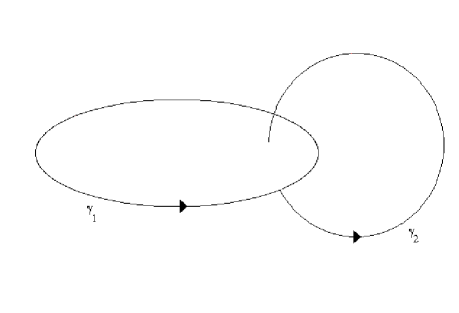
Figure 1:

As is well known, the linking number $\chi(\gamma_{1},\gamma_{2})$ is an integer which counts the number of times that one curve winds around the other. It is independent from the shape of the curves and can be represented by the Gauss integral

$$\chi(\gamma_{1},\gamma_{2})=\frac{1}{4\pi}\oint_{\gamma_{1}}dx^{\mu}\oint_{\gamma_{2}}dy^{\nu}\varepsilon_{\mu\nu\rho}\frac{(x-y)^{\rho}}{\left|x-y\right|^{3}}\;.$$ (1)

Expression (1) is in fact easily seen to be an integer by use of the Stokes’ theorem [3, 4]. Taking a field theory point of view, the linking number $\chi(\gamma_{1},\gamma_{2})$ may be obtained by introducing the topological abelian Chern–Simons action [1]

$$\mathcal{S}_{\mathrm{CS}}(A)=\frac{1}{2}\int d^{3}x\varepsilon^{\mu\nu\rho}A_{\mu}\partial_{\nu}A_{\rho}\;,$$ (2)

and by evaluating the correlation function of two loop variables $\oint_{\gamma}dx^{\mu}A_{\mu}$, i..e.,

$$\left\langle\oint_{\gamma_{1}}dx^{\mu}A_{\mu}\oint_{\gamma_{2}}dy^{\nu}A_{\nu}\right\rangle_{\mathcal{S}_{\mathrm{CS}}}\;.$$ (3)

That expression (3) reproduces the linking number follows from the observation that the propagator of the gauge field $A_{\mu}$ obtained from the Chern–Simons action (2) upon quantization in the Landau gauge is precisely the kernel of the Gauss integral (1), i.e.,

$$\left\langle A_{\mu}(x)A_{\nu}(y)\right\rangle_{\mathcal{S}_{\mathrm{CS}}}=\frac{1}{4\pi}\varepsilon_{\mu\nu\rho}\frac{(x-y)^{\rho}}{\left|x-y\right|^{3}}\;.$$ (4)

The correlator (3) may thus be regarded as a field-theory description of the linking $\chi(\gamma_{1},\gamma_{2}).$ The action (2) can be suitably extended to higher dimensions, providing a field-theory characterization of the generalizations of the linking number [4]. Moreover, the nonabelian version of the three-dimensional Chern–Simons action (2) has been proven to play a very relevant role in knot theory [1, 3].

Although the topological field theories possess their own interests and applications, it is worth underlining here that topological terms appear frequently as parts of more general effective actions useful for the theoretical description of a large number of phenomena in different space-time dimensions. For instance, the effective action corresponding to the bosonization [5] of relativistic three-dimensional massive fermionic systems at $T=0$ can be written as the sum of the Chern-Simons term (2) and of an infinite series of higher-order terms in the curvature $F_{\mu\nu}$ and its derivatives, i.e.,

$$\mathcal{S}_{\mathrm{CS}}(A)+\mathcal{S}(F),\;$$ (5)

with $\mathcal{S}(F)$ being a combination of terms of the type

$$\int d^{3}xF^{2},\;\int d^{3}xF^{4},\;\int d^{3}xF^{6},\;\ldots$$ (6)

This kind of action turns out to be useful in order to study several three-dimensional phenomena such as the Fermi–Bose transmutation [6, 7] and the quantum Hall effect [8].

A second interesting example is provided by the five-dimensional generalization of (5), obtained from the AdS/CFT correspondence [9, 10], which relates the conformal $N=4$ super-Yang-Mills theory to type-IIB superstring on AdS${}_{5}\times S^{5}$. In fact, in the conformal case, the dual supergravity on $AdS_{5}$ possesses a Chern–Simons term obtained from a $SL(2,\mathbb{Z})$ doublet of two-forms $B_{\mu\nu}^{RR},$ $B_{\mu\nu}^{NS}$. In this case, the relevant effective action for $B_{\mu\nu}^{RR},$ $B_{\mu\nu}^{NS}$ looks like [10]

$$\int_{\rm{AdS}_{5}}d^{5}x\varepsilon^{\mu\nu\rho\lambda\sigma}B_{\mu\nu}^{RR}\partial_{\rho}B_{\lambda\sigma}^{NS}\;+\mathcal{S}(dB)\;,$$ (7)

where the term $\mathcal{S}(dB)$ collects all the higher-order terms in the curvatures $dB^{RR},dB^{NS}$. The correlation function (3) generalizes now to

$$\left\langle\int_{\Sigma_{1}}d\sigma^{\mu\nu}B_{\mu\nu}^{RR}\int_{\Sigma_{2}}d\sigma^{\lambda\rho}B_{\lambda\rho}^{NS}\right\rangle\;,$$ (8)

where $\Sigma_{1},$ $\Sigma_{2}$ are appropriate two-surfaces.

In view of these applications, it seems natural to ask ourselves what is the response of a correlator of the type (3) when the corresponding topological field theory is perturbed by the introduction of a nontopological interaction term depending on the curvature.

This is the aim of the present paper. More precisely, we shall report on the four-loop computation of the correlator

$$\left\langle\oint_{\gamma_{1}}dx^{\mu}A_{\mu}\oint_{\gamma_{2}}dy^{\nu}A_{\nu}\right\rangle_{\mathcal{S}_{\mathrm{eff}}}\;,$$ (9)

when the three-dimensional Chern–Simons action (2) is perturbed by a nontopological interaction term of the kind $\int F^{4},$ namely, expression (9) will be evaluated with an effective action $\mathcal{S}_{\mathrm{eff}}$ given by

$$\mathcal{S}_{\mathrm{eff}}=\frac{1}{2}\int d^{3}x\varepsilon^{\mu\nu\rho}A_{\mu}\partial_{\nu}A_{\rho}+\frac{\tau}{4!}\int d^{3}x\widetilde{F}^{\mu}\widetilde{F}_{\mu}\widetilde{F}^{\nu}\widetilde{F}_{\nu}\;,$$ (10)

with $\widetilde{F}^{\mu}=\frac{1}{2}\varepsilon^{\mu\nu\rho}F_{\nu\rho}$ and $\tau$ being an arbitrary parameter with negative mass dimension, reflecting the power-counting nonrenormalizability of the perturbation.

In particular, we shall be able to prove that the correlation function (9) turns out to be independent from $\tau$, yielding the linking number $\chi(\gamma_{1},\gamma_{2})$ of the two curves $\gamma_{1}$, $\gamma_{2}.$ Although the loop analysis will be worked out only up to the fourth order, this conclusion holds to all orders of perturbation theory and may be easily generalized to any local nontopological interaction term containing arbitrary powers of the curvature $F_{\mu\nu}$ as well as to the higher-dimensional cases [11] as, for instance, the effective action of eq.(7).

This result means that the loop correlator (9) is stable with respect to the perturbations which can be added to the starting topological action. In other words, the expression (9) will give the linking number of the two curves $\gamma_{1}$, $\gamma_{2}$, regardless of any $F$-dependent perturbation term that can be introduced and of their power-counting nonrenormalizability character.

Two remarks are now in order. First, we will limit here ourselves only to effective actions which are abelian. Second, we shall consider only $F$-dependent terms which can be treated as true perturbations. Therefore, we shall avoid in the effective action (10) the inclusion of a term of the Maxwell type

$$\mathcal{S}_{\mathrm{Max}}=\frac{1}{4m}\int d^{3}xF^{\mu\nu}F_{\mu\nu}\;,$$ (11)

where $m$ is a mass parameter. The presence of this term would completely modify the original properties of the model. In fact, being expression (11) quadratic in the gauge fields, it cannot be considered as a perturbation term, as it will be responsible for the presence of massive excitations in the spectrum of the theory [12]. Rather, the presence of the Maxwell term in the effective action (10) will give rise to the existence of two distinct regimes corresponding to the long and short distance behaviours, respectively. For distances larger than the inverse of the mass parameter $m$ (i.e., the low-energy regime ), the topological term will prevail, while the Maxwell term will become the relevant one at short distances (i.e., the high-energy regime). It is worth mentioning here that these two regimes can be accessed in a very simple way by means of suitable gauge-invariant field redefinitions of the gauge connection $A_{\mu}$ [13]. However, their full understanding is a difficult and delicate task, which is beyond the aim of the present paper, being under investigation.

We should also underline here that, in the abelian case, the loop variable $\oint_{\gamma}dx^{\mu}A_{\mu}$ is gauge invariant for closed curves, and so there is no need to take into account its exponentiation $e^{i\oint_{\gamma}dx^{\mu}A_{\mu}}$, as it would be required in the nonabelian case. This feature has a useful consequence. It allows indeed to avoid the case in which the double-line integral (9) has to be taken along the same curve. This case, usually referred to as the self-linking, would be automatically generated by the perturbative Taylor expansion of the exponential $e^{i\oint_{\gamma}dx^{\mu}A_{\mu}}$. In other words, as far as the abelian case is concerned, the loop variables in eq.(9) do not need to be exponentiated. Therefore, the two curves $\gamma_{1}$ and $\gamma_{2}$ will always refer to two distinct curves which do not intersect each other. As we shall see in the following, this point will be relevant in order to establish the independence from the parameter $\tau$ of the expression (9).

2 Perturbative expansion and Feynman diagrams

In order to discuss the perturbative expansion of the loop correlator (9), let us first define the gauge-fixed version of the effective action which shall be used throughout the present article, namely,

$$\mathcal{S}_{\mathrm{eff}}=\frac{1}{2}\int d^{3}x\varepsilon^{\mu\nu\rho}A_{\mu}\partial_{\nu}A_{\rho}+\int d^{3}x\,b\partial A+\frac{\tau}{4!}\int d^{3}x:\widetilde{F}^{\mu}\widetilde{F}_{\mu}\widetilde{F}^{\nu}\widetilde{F}_{\nu}:\,,$$ (12)

where the Lagrange multiplier $b$ has been introduced in order to implement the Landau gauge. Notice that we have Wick-ordered the quartic interaction term, which will allow to rule out tadpole diagrams.

As usual in this kind of problem, we shall make use of the configuration space rather than the momentum space. Let us now give the elementary Wick contractions which shall be needed for the evaluation of the Feynman diagrams. Recalling that

$$\partial^{2}\frac{1}{\left|x-y\right|}=-4\pi\delta^{3}(x-y)\;,$$ (13)

from eq.(4) one obtains

$$\left\langle A_{\mu}(x)\widetilde{F}_{\nu}(y)\right\rangle=g_{\mu\nu}\delta^{3}(x-y)+\partial_{\mu}\partial_{\nu}\frac{1}{4\pi\left|x-y\right|}\;,$$ (14)

and

$$\left\langle\widetilde{F}_{\mu}(x)\widetilde{F}_{\nu}(y)\right\rangle=-\varepsilon_{\mu\nu\rho}\partial^{\rho}\delta^{3}(x-y)\;.$$ (15)

Concerning now the perturbative loop expansion, it is easily checked that the first Feynman diagram which contributes to the correlation function (9) is of two-loop order and can be drawn as follows:

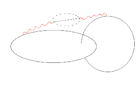
Figure 2: Two-loop contribution

In the above figure, the wavy and dashed lines refer respectively to the Wick contractions $\left\langle A\widetilde{F}\right\rangle$ and $\left\langle\widetilde{F}\widetilde{F}\right\rangle$.

The Feynman integrals corresponding to the diagram of Fig.2 are easily written down by means of eqs.(14), (15). However, before computing them, let us spend a few words on the mechanism which is responsible for the independence on the parameter $\tau$ of expression (9). From the structure of the diagram of Fig.2, we observe that the gauge fields $A_{\mu}(x)$ and $A_{\nu}(y)$ lying on the two curves $\gamma_{1}\;$and $\gamma_{2\rm{}}$will be always contracted with the $\widetilde{F}$’s present in the interaction term of the expression (12). Therefore, besides contractions of the type $\left\langle\widetilde{F}\widetilde{F}\right\rangle$, the corresponding Feynman integrals will always contain two contractions of the kind $\left\langle A\widetilde{F}\right\rangle$. However, one should remark in the second term of eq.(14) that one of the Lorentz indices of the two space-time derivatives corresponds to the vector index of a gauge field lying on either $\gamma_{1}\;$or $\gamma_{2}.$ It thus refers to a total derivative with respect to the variable running along one of the closed loops, implying a vanishing contribution. In other words, the second term of eq.(14) may be neglected. As a consequence, all the Wick contractions entering the Feynman integrals will basically lead to a product of delta functions. After the introduction of a suitable regularization, the latter can be integrated out, finally resulting in a $\delta^{3}(x-y)$, where, we remind, $x$ and $y$ run along each of the two curves, respectively. As these variables never coincide, the whole expression vanishes identically, ensuring the independence from the parameter $\tau$ of the correlator (9). The same mechanism can be seen to occur at higher loop orders, as it will be explicitly shown later on.

Apart from an irrelevant global symmetry coefficient, the diagram of Fig.2 therefore corresponds to the following integral:

$$I^{(2)}\!\!\! = \!\!\!\oint_{\gamma_{1}}dx^{\mu}\oint_{\gamma_{2}}dy^{\nu}\int d^{3}z_{1}\,d^{3}z_{2}\,\left\langle A_{\mu}(x)\tilde{F}_{\alpha}(z_{1})\right\rangle\left\langle A_{\nu}(y)\tilde{F}_{\gamma}(z_{2})\right\rangle\left\langle\tilde{F}_{\beta}(z_{1})\tilde{F}_{\rho}(z_{2})\right\rangle$$ (16)

$$\!\!\!\!\!\!\times\left[4\left\langle\tilde{F}^{\alpha}(z_{1})\tilde{F}^{\rho}(z_{2})\right\rangle\left\langle\tilde{F}^{\beta}(z_{1})\tilde{F}^{\gamma}(z_{2})\right\rangle+2\left\langle\tilde{F}^{\alpha}(z_{1})\tilde{F}^{\gamma}(z_{2})\right\rangle\left\langle\tilde{F}^{\beta}(z_{1})\tilde{F}^{\rho}(z_{2})\right\rangle\right].$$

Let us analyse the first term of the above expression. Making use of the propagators (14) and (15), we obtain

$$-4\oint_{\gamma_{1}}dx^{\mu}\oint_{\gamma_{2}}dy^{\nu}\int d^{3}z_{1}\,d^{3}z_{2}\,$$

$$\quad\times\left[g_{\mu\alpha}\delta^{3}(x-z_{1})+\partial_{\mu}\partial_{\alpha}\frac{1}{4\pi\left|x-z_{1}\right|}\right]\left[g_{\nu\gamma}\delta^{3}(y-z_{2})+\partial_{\nu}\partial_{\gamma}\frac{1}{4\pi\left|y-z_{2}\right|}\right]$$

$$\quad\times\left[\varepsilon_{\beta\rho\lambda}\partial^{\lambda}\delta^{3}(z_{1}-z_{2})\right]\left[\varepsilon^{\alpha\rho\tau}\partial_{\tau}\delta^{3}(z_{1}-z_{2})\right]\left[\varepsilon^{\beta\gamma\sigma}\partial_{\sigma}\delta^{3}(z_{1}-z_{2})\right]\,.$$ (17)

As previously mentioned, the terms containing the derivatives $\partial_{\mu}$ and $\partial_{\nu}$ do not contribute, as they correspond to total derivatives on closed curves. Expression (17) then becomes

$$4\oint_{\gamma_{1}}dx^{\mu}\oint_{\gamma_{2}}dy^{\nu}\int d^{3}z_{1}\,d^{3}z_{2}\,\delta^{3}(x-z_{1})\delta^{3}(y-z_{2})$$

$$\quad\times\left[\varepsilon_{\beta\rho\lambda}\partial^{\lambda}\delta^{3}(z_{1}-z_{2})\right]\left[\varepsilon_{\mu}{}^{\rho\tau}\partial_{\tau}\delta^{3}(z_{1}-z_{2})\right]\left[\varepsilon^{\beta\sigma}{}_{\nu}\partial_{\sigma}\delta^{3}(z_{1}-z_{2})\right]\,.$$ (18)

In spite of the presence of products of delta functions with the same arguments, the above expression is easily seen to vanish. Let us show this claim in two ways. First, we observe that there is always a possible order of taking the integrations over the delta functions such that we end up with products of $\delta^{3}(x-y)$ and not of $\delta^{3}(0)$. In the present case, this would amount to integrate out first the two delta functions with arguments $x-z_{1}$ and $y-z_{2}$, which would lead to

$$4\oint_{\gamma_{1}}dx^{\mu}\oint_{\gamma_{2}}dy^{\nu}\left[\varepsilon_{\beta\rho\lambda}\partial^{\lambda}\delta^{3}(x-y)\right]\left[\varepsilon_{\mu}{}^{\rho\tau}\partial_{\tau}\delta^{3}(x-y)\right]\left[\varepsilon^{\beta\sigma}{}_{\nu}\partial_{\sigma}\delta^{3}(x-y)\right]=0\,,$$ (19)

since $x-y$ never vanishes. It is worth remarking that this possibility exists, in fact, for the higher-order diagrams, as will be shown below.

Second, we can adopt a more rigorous treatment by regularizing the delta functions with coinciding arguments through the point-splitting procedure already used by Polyakov [6]:

$$\delta_{\varepsilon}(z_{1}-z_{2}) = \frac{1}{\left(2\pi\varepsilon\right)^{3/2}}e^{-(z_{1}-z_{2})^{2}/2\varepsilon}\,,$$ (20)

$$\lim_{\varepsilon\rightarrow 0}\delta_{\varepsilon}(z_{1}-z_{2}) = \delta^{3}(z_{1}-z_{2})\;.$$

More precisely, whenever a product of $n$ delta functions with coinciding arguments occurs, it will be understood as

$$\left[\delta^{3}(z_{1}-z_{2})\right]^{n}=\left[\delta_{\varepsilon}(z_{1}-z_{2})\right]^{n-1}\delta^{3}(z_{1}-z_{2})\,,$$

where the limit $\varepsilon\rightarrow 0$ is meant to be taken at the end of all calculations. Accordingly, expression (18) will be replaced by its regularized version,

$$\lim_{\varepsilon\rightarrow 0}4\oint_{\gamma_{1}}dx^{\mu}\oint_{\gamma_{2}}dy^{\nu}\,\delta^{3}(x-z_{1})\delta^{3}(y-z_{2})$$

$$\quad\times\left[\varepsilon_{\beta\rho\lambda}\partial^{\lambda}\delta_{\varepsilon}(z_{1}-z_{2})\right]\left[\varepsilon_{\mu}{}^{\rho\tau}\partial_{\tau}\delta_{\varepsilon}(z_{1}-z_{2})\right]\left[\varepsilon^{\beta\sigma}{}_{\nu}\partial_{\sigma}\delta^{3}(z_{1}-z_{2})\right]\,.$$ (21)

Whatever the order of integration, we get, before taking the limit, an expression containing $\delta^{3}(x-y)$, which leads to a null result.

The second term of (16) follows analogously, so that the two-loop diagram of Fig.2 does not contribute to the correlator (9).

Concerning the higher-order contributions in the perturbation theory, the results are of a similar nature. The topologically distinct diagrams contributing to the 3- and 4-loop are given in Fig.3 and in Figs.4 and 5.

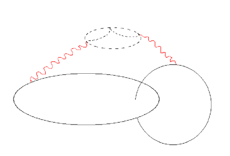
Figure 3: Three-loop contribution

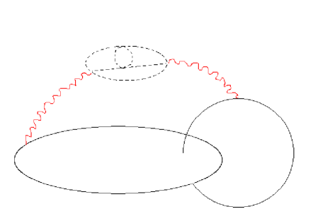
Figure 4: Four-loop contribution, first type

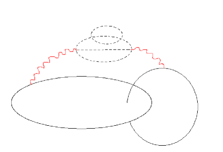
Figure 5: Four-loop contribution, second type

It is sufficient to present here just one typical term of each order. A notational simplification is convenient. We define the transverse derivative operator

$$\tilde{\partial}_{\mu\nu}\equiv\varepsilon_{\mu\nu\rho}\partial^{\rho}.$$

For instance, a typical contraction from Fig.3 is proportional to

$$I^{(3)} = \oint_{\gamma_{1}}dx^{\mu}\oint_{\gamma_{2}}dy^{\nu}\int d^{3}z_{1}\,d^{3}z_{2}d^{3}z_{3}\,g_{\mu\alpha}\delta^{3}(x-z_{1})g_{\nu\gamma}\delta^{3}(y-z_{2})$$

$$\times\left[\tilde{\partial}^{\alpha\gamma}\delta^{3}(z_{1}-z_{2})\right]\left[\tilde{\partial}_{\beta\delta}\delta^{3}(z_{1}-z_{3})\right]\left[\tilde{\partial}^{\beta\lambda}\delta^{3}(z_{1}-z_{3})\right]$$

$$\times\left[\tilde{\partial}_{\rho\lambda}\delta^{3}(z_{2}-z_{3})\right]\left[\tilde{\partial}^{\rho\delta}\delta^{3}(z_{2}-z_{3})\right]$$

$$= \oint_{\gamma_{1}}dx^{\mu}\oint_{\gamma_{2}}dy^{\nu}\int d^{3}z_{3}\left[\tilde{\partial}_{\mu\nu}\delta^{3}(x-y)\right]$$

$$\times\left[\tilde{\partial}_{\beta\delta}\delta_{\varepsilon}(x-z_{3})\right]\left[\tilde{\partial}^{\beta\lambda}\delta^{3}(x-z_{3})\right]\left[\tilde{\partial}_{\rho\lambda}\delta_{\varepsilon}(y-z_{3})\right]\left[\tilde{\partial}^{\rho\delta}\delta^{3}(y-z_{3})\right],$$

while the diagram of Fig.4 gives

$$I^{(4)} = \oint_{\gamma_{1}}dx^{\mu}\oint_{\gamma_{2}}dy^{\nu}\int d^{3}z_{1}\cdots d^{3}z_{4}\,g_{\mu\alpha}\delta^{3}(x-z_{1})g_{\nu\gamma}\delta^{3}(y-z_{2})$$ (23)

$$\times\left[\tilde{\partial}^{\alpha\gamma}\delta^{3}(z_{1}-z_{2})\right]\left[\tilde{\partial}^{\beta\lambda}\delta^{3}(z_{1}-z_{3})\right]\left[\tilde{\partial}_{\beta\sigma}\delta^{3}(z_{1}-z_{4})\right]$$

$$\times\left[\tilde{\partial}^{\rho\sigma}\delta^{3}(z_{2}-z_{4})\right]\left[\tilde{\partial}_{\rho\lambda}\delta^{3}(z_{2}-z_{3})\right]\left[\tilde{\partial}^{\varphi\omega}\delta^{3}(z_{3}-z_{4})\right]$$

$$\times\left[\tilde{\partial}_{\varphi\omega}\delta^{3}(z_{3}-z_{4})\right]$$

$$= \oint_{\gamma_{1}}dx^{\mu}\oint_{\gamma_{2}}dy^{\nu}\int d^{3}z_{3}\,d^{3}z_{4}\,\left[\tilde{\partial}_{\mu\nu}\delta^{3}(x-y)\right]$$

$$\times\left[\tilde{\partial}^{\beta\lambda}\delta^{3}(x-z_{3})\right]\left[\tilde{\partial}_{\beta\sigma}\delta^{3}(x-z_{4})\right]\left[\tilde{\partial}^{\rho\sigma}\delta^{3}(y-z_{4})\right]$$

$$\times\left[\tilde{\partial}_{\rho\lambda}\delta^{3}(y-z_{3})\right]\left[\tilde{\partial}^{\varphi\omega}\delta_{\varepsilon}(z_{3}-z_{4})\right]\left[\tilde{\partial}_{\varphi\omega}\delta^{3}(z_{3}-z_{4})\right].$$

In order to obtain the above expressions we have followed the same prescription established before for regularizing the delta functions with identical arguments. Notice also that we have integrated out first the two $\delta$-functions whose arguments depend on the points $x$ and $y$ of the two curves.

All terms in all possible diagrams may then be seen to be proportional to $\delta^{3}(x-y)$ (or its derivatives). One may easily convince oneself that this mechanism also applies to any order in perturbation theory. As we always have $x\neq y$, these diagrams all amount to a null correction to the basic diagram, so that the correlation function (9) for two closed smooth nonintersecting curves $\gamma_{1},\gamma_{2}$ gives their linking number to all orders:

$$\left\langle A_{\mu}(x)A_{\nu}(y)\right\rangle_{\mathcal{S}_{\rm{eff}}}=\chi(\gamma_{1},\gamma_{2}).$$ (24)

3 Conclusions

We have been able to show, in the present article, that the correlation function (9) is unaffected by the radiative corrections, provided $\gamma_{1},\gamma_{2}$ are two nonintersecting closed curves. Although we have given explicit expressions for the $\int\tilde{F}^{4}$ perturbation, the same result may be achieved for any local interaction term of the type $\int\tilde{F}^{n}$.

We may interpret this result as a kind of nonrenormalization property of the linking number, reflecting its stability with respect to any local gauge invariant perturbation of the starting Chern-Simons action.

Further generalizations to higher dimensions as well as to the nonabelian case are under investigation [11].

Acknowledgements

The Conselho Nacional de Pesquisa e Desenvolvimento (CNPq/Brazil), the Fundação de Amparo à Pesquisa do Estado do Rio de Janeiro (Faperj) and the SR2-UERJ are gratefully acknowledged for financial support.

References

- [1] E. Witten, Comm. Math. Phys. 117 (1988) 353; Comm. Math. Phys. 118 (1988) 411; Comm. Math. Phys. 121 (1988) 351.
- [2] D. Birmingham, M. Blau, M. Rakowski and G. Thompson, Phys. Rep. 209 (1991) 129.
- [3] E. Guadagnini, The Link Invariants of the Chern–Simons Field Theory, De Gruyter, Berlin and New York, 1993.
- [4] C. H. Tze and S. Nam, Ann. Phys. 193 (1989) 419.
-
[5]
E. C. Marino, Phys. Lett. B 263 (1991) 63;
E. Fradkin and F.A. Schaposnik, Phys. Lett. B 338 (1994) 253;
F. A. Schaposnik, Phys. Lett. B 356 (1995) 39;
C. P. Burgess, C. A. Lütken and F. Quevedo, Phys. Lett. B 336 (1994) 18;
D. G. Barci, C.D. Fosco and L. E. Oxman, Phys. Lett. B 375 (1996) 267;
R. Banerjee and E.C. Marino, Nucl. Phys. B 507 (1997) 501. - [6] A.M. Polyakov, Mod. Phys. Letters A 3 (1988) 325.
-
[7]
T.H. Hansson, A. Karlhede and M. Rocek, Phys. Lett. B
225 (1989) 92.
N. Bralić and L. Vergara, Fuzzy Statistics in Covariant Quantum Field Theory, Int. Europhys. Conf. on High Energy Physics, Marseille, France, 1993. - [8] E. Fradkin, Field Theories of Condensed Matter Systems, Addison-Wesley Publishing Company, Frontiers in Physics; 82, 1991.
- [9] J. Maldacena, The Large N Limit of Superconformal Field Theories and Supergravity, hep-th/9711200.
- [10] E. Witten, AdS/CFT Correspondence and Topological Field Theory, hep-th/9812012.
- [11] Work in progress.
- [12] S. Deser, R. Jackiw and S. Templeton, Ann. Phys. 140 (1982) 372.
- [13] V.E.R. Lemes, C.A. Linhares, S.P. Sorella and L.C.Q. Vilar, Large-mass behaviour of loop variables in abelian Maxwell-Chern-Simons theory, hep-th/9804186, to appear in J. Phys. A: Math. Gen.