Holographic View of Causality and Locality

via

Branes in AdS/CFT Correspondence 

Dongsu Bak¹      &      Soo-Jong Rey²

Physics Department, University of Seoul, Seoul 130-743 Korea¹

Physics Department, Seoul National University, Seoul 151-742 Korea²

dsbak@mach.uos.ac.kr,  sjrey@gravity.snu.ac.kr

abstract

We study dynamical aspects of holographic correspondence between $d=5$ anti-de Sitter supergravity and $d=4$ super Yang-Mills theory. We probe causality and locality of ambient spacetime from super Yang-Mills theory by studying transmission of low-energy brane waves via an open string stretched between two D3-branes in Coulomb branch. By analyzing two relevant physical threshold scales, we find that causality and locality is encoded in the super Yang-Mills theory provided infinite tower of long supermultiplet operators are added. Massive W-boson and dual magnetic monopole behave more properly as extended, bilocal objects. We also study causal time-delay of low-energy excitation on heavy quark or meson and find an excellent agreement between anti-de Sitter supergravity and super Yang-Mills theory descriptions. We observe that strong ‘t Hooft coupling dynamics and holographic scale-size relation thereof play a crucial role to the agreement of dynamical processes.

1 Introduction

It is now widely believed that an anti-de Sitter (AdS) supergravity is dual to large N limit of conformal field theory (CFT) [1]. A particularly interesting case of this so-called AdS/CFT correspondence is between semiclassical limit of Type IIB superstring compactified to five-dimensional anti-de Sitter spacetime and large-$N$ limit of super Yang-Mills theories in four dimensions. As exemplified by this case, one of the most important features is that the ‘holographic principle’ [2, 3, 4] underlies all AdS/CFT correspondences: semi-classical gravity in $(d+1)$ dimensions is holographically is described by degrees of freedom of large-$N$ quantum field theory in $d$-dimensions. The AdS/CFT correspondence has been test extensively and evidence for it has been drawn mainly from agreement between the two sides of various static quantities, such as symmetries, particle spectrum, correlation functions, and black hole entropy [5, 6, 7].

The holographic principle, however, refers to the correspondence not just for static properties only but also for all dynamical ones . This raises an immediate puzzle: how can possibly local and causal dynamics on anti-de Sitter spacetime be recovered from a lower-dimensional quantum field theory? Large-$N$ super Yang-Mills theory is certainly a well-defined quantum field theory [15] with locality and causality of four-dimensional Minkowski spacetime built in. So is the supergravity in anti-de Sitter spacetime, in the semi-classical limit at the least. Given the apparent locality and causality of physics, it seems virtually impossible to describe what happens in the bulk of spacetime by dynamical variables located at the boundary. In this paper, taking the correspondence between Type IIB superstring on $d=5$ anti-de Sitter spacetime and $d=4$ super Yang-Mills theory as a setup, we will try to provide an answer to this puzzle.

More specifically, we will pose and study the following question: in order to encode causality and locality of semi-classical supergravity in $d=5$ anti-de sitter spacetime, what precise prescription does one need in formulating the $d=4$ super Yang-Mills theory? Our main conclusion will be that neither conventional (keeping dimension-four operators only) nor Dirac-Born-Infeld form is sufficient and only after infinite tower of higher-dimensional operators encompassing long supermultiplets are included, causality and locality can be decoded out of the super Yang-Mills theory.

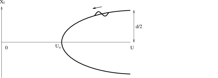
We will address the posed question in the Coulomb branch of the super Yang-Mills theory, viz. consider $SU(N)\rightarrow S[U(N-2)\times(U(1)\times U(2))]$ by separating two D3-branes out of the $(N-2)$ remainder and place them at $r_{1,2}$, respectively, in the Coulomb branch moduli space. We will then place a macroscopic open string (either fundamental or Dirichlet) stretched between the two D3-branes and study transmission of localized brane waves from the first D3-brane to the second through the string. The stretched open string is identified with a massive W-boson with mass $M_{\rm w}=(r_{1}-r_{2})\equiv\Delta r$. As the string is stretched over a distance $\Delta r$, under suitable circumstance, one would expect to detect causal time-delay out of the transmitted brane-waves.

This process, which is a sort of Thomson scattering [16] (alias Compton scattering at low-energy) of brane waves off a massive W-boson, is closely related to much-studied, $F^{4}$ brane-wave interaction [17, 18, 19, 20, 21, 22]. Cutting the one-loop diagram of the latter across two internal W-boson lines, one obtains a pair of tree-level, Thomson scattering diagram. In so far as probing causality and locality, the only difference between the two would be that the $F^{4}$ brane-wave interaction describes inter-brane interaction via exchange of closed string states, while the Thomson scattering interaction describes interaction via virtual excitation of the massive W-boson. In effect, the stretched open string serves as a sort of one-dimensional ‘waveguide’ of the radiation, which would otherwise have propagated out all over ambient spacetime.

Comparison of Thomson scattering with known results regarding $F^{4}$ brane-wave interaction brings up another important lesson drawn throughout this work: static and dynamic information are closely related in flat spacetime, but not in anti-de Sitter spacetime. In flat spacetime (corresponding to $N=2$), it is well-known that the $F^{4}$ brane-wave interaction is exact at one-loop by the non-renormalization theorem of [18]. Douglas and Taylor [23] have argued that, by taking a coincident $(N-2)$-brane limit from a generic point in the Coulomb branch, the non-renormalization theorem should also hold in anti-de Sitter spacetime. As an evidence for this assertion, they have noted that, the supergravity interaction for zero-momentum brane waves is the same for both flat and anti-de Sitter spacetime. Through careful analysis, Das [24] has confirmed the result further . The interaction at zero-momentum, however, is always instantaneous and retarded interaction will show up only if nonzero momentum configuration is considered, a well-known fact of nonrelativistic expansion in covariant perturbation theory. For brane waves with nonzero momentum, corrections to the leading order result in Yang-Mills theory is controlled by the string scale, $\ell_{s}$ [23], hinting that stringy corrections somehow ought to be taken into account to the supergravity description. Douglas and Taylor have interpreted these corrections as a manifestation of the spacetime uncertainty principle [25]. Das has sketched calculation of retarded interaction between nonzero momentum brane waves in flat spacetime and have argued that the non-renormalization theorem assures the same result in anti-de Sitter spacetime. Underlying to their arguments seems that the massive W-boson, which is a stretched open string of length $\Delta r$, is a good ruler for measuring distance and hence causality of the bulk spacetime, both flat and anti-de Sitter.

From Thomson scattering process, we will find contrasting results. Underlying to the process, the W-boson, being an open string stretched between the two D3-branes, sets two competing threshold scales: winding and oscillation energy of the string. We will find that causality and locality of the ambient spacetime is visible in super Yang-Mills theory only if the oscillation threshold is lighter than the winding threshold. The winding threshold remains the same for both flat and anti-de Sitter spacetime but, quite importantly, the oscillation threshold turns out to change significantly . In flat spacetime, crossover between the two threshold takes place when $\Delta r\sim{\cal O}(\ell_{s})$, confirming from dynamical side the well-known result on D-brane worldvolume dynamics [26]. In anti-de Sitter spacetime, however, crossover takes place when (using Maldacena’s scaling variable $U\equiv r/\ell_{s}^{2}$)

$${(\Delta U)^{2}\over U_{1}U_{2}}\qquad\sim\qquad{\cal O}\left({1\over g_{\rm st}N}\right).$$ (1.1)

It shows that, everywhere in the Coulomb branch (possibly except at the origin), stong ‘t Hooft coupling limit ensures that the oscillation threshold is lower than the winding threshold and hence enables the large-$N$ super Yang-Mills theory to encode causality and locality of semi-classical supergravity in the anti-de Sitter spacetime.

With light oscillation threshold, the super Yang-Mills theory is given in a rather different form from conventional (retaining dimension-four operators only) or Dirac-Born-Infeld theories. The massive W-bosons and dual magnetic monopoles are more suitably described as a sort of extended, bilocal object . Remarkably, particle Lagrangian of the W-boson takes (an extended form of) Pais-Uhlenbeck [28] model with transcendental, infinite-order kernels, which is one of the few known examples satisfying convergence, positive-definiteness and strict causality.

This paper is organized as follows. In section 2, we will study brane-wave transmission via Thomson scattering, first in flat spacetime. In section 3, we will study the holographic relation between energy and size in AdS/CFT correspondence, but now from dynamical point of view. We will be studying causal time delay of low-energy excitations added to a macroscopic string representing quark or meson [30, 31]. We will find an excellent agreement between anti-de Sitter supergravity and super Yang-Mills theory results. In section 4, we will study brane-wave transmission via Thomson scattering, but now in anti-de Sitter spacetime. In appendix A and B, we will explain technical details of covariant Green-Schwarz action for open string stretched between the two D3-branes, in particular, consistent gauge-fixing of $\kappa$-symmetry. We will also derive a low-energy effective Lagrangian for bilocal W-boson, for both flat and anti-de Sitter spacetimes.

2 Causality and Locality in Flat Spacetime

Before dwelling into anti-de Sitter spacetime, we will first study causality and locality in flat spacetime. To make a direct comparison with anti-de Sitter spacetime later, as a probe, we will use a system consisting of two D3-branes and a open F- or D-string stretched between them.

Consider, in Type IIB string theory, two parallel D3-branes in flat spacetime $X={\bf R}^{9,1}$. The D3-branes are oriented along $0,1,2,3$ directions and are located along $4,\cdots,9$ directions at $(r_{1},0,\cdots,0)$ and $(r_{2},0,\cdots,0)$, respectively. Low-energy dynamics on the D3-brane worldvolume is governed by $d=4,{\cal N}=4$ super Yang-Mills theory with gauge group $G=U(2)$. We will denote generators of $U(2)$ gauge group as $T_{a}$ $(a=1,2,3,4)$, where $T_{1,2,3}=\sigma_{1,2,3}$ belong to the $SU(2)$ and $T_{4}=id$ to the diagonal $U(1)$ subgroups. As the two D3-branes are separated by a distance $\Delta r=|r_{1}-r_{2}|$, the $SU(2)$ gauge group is spontaneously broken to $U(1)$ generated by $T_{3}$ Cartan subalgebra. Together with the diagonal $U(1)$, the gauge group on the two D3-branes, which we label by 1 and 2, is then given by $H=U^{(1)}(1)\times U^{(2)}(1)$, generated by diagonal linear combinations, $(T_{3}\pm T_{4})/2$. A massive W-boson (or dual magnetic monopole) associated with the spontaneous symmetry breaking is represented by an open F-string (or D-string) stretched between the two D3-branes. The static mass of the W-boson and the dual magnetic monopole is given by

$$M_{\rm w}=T\Delta r,\qquad M_{\rm m}={T\over g_{\rm st}}\Delta r.$$ (2.2)

They are part of an isospin triplet under $G$ (or its dual gauge group) and hence, under $H$, carry electric (or magnetic) charges $(Q,-Q)$ where $Q=\pm 1$ .

To investigate causality and locality of the flat Minkowski spacetime over the distance scale $\Delta r$, one will need to excite slightly, say, the first D3-brane and follow subsequent propagation of the excitation, which will eventually arrive at and excite the second D3-brane. In the limit $g_{\rm st}\rightarrow 0$, semi-classical dynamics of the Type IIB supergravity ought to obey both locality and causality. For low-energy excitation, the leading order process in this limit will be such that the excitation is transmitted from the first D3-brane to the second through an open F- or D-string stretched between them . When exciting brane-wave on the first D3-brane, there are two channels available: massless Higgs or $U^{(1)}(1)$ gauge field waves. In what follows, we will consider exclusively adding a weak amplitude, plane-wave of the $U^{(1)}(1)$ gauge field on the first D3-brane . The entire dynamical process is then viewed as the classic, Thomson scattering of the $U^{(1)}(1)$ radiation field off the open string.

The open string stretched between the two D3-branes is casually identified with a massive W-boson. This sounds paradoxical since the open string is an extended object whose characteristic scale is the string scale, $\ell_{s}$, while the massive W-boson is a point-like object. An answer to this is well-known [26] ever since the advent of the D-branes. In this section, from the dynamical point of view, we will revisit this issue as it is intimately tied with understanding causality and locality of the ambient spacetime in which the D-branes are embedded. Specifically, we will study the Thomson scattering process in two opposite limits of the massive W-boson, first in a point-particle limit and second in a stretched open string limit. We will find shortly that, over the distance scale $\Delta r$, super Yang-Mills theory will perceive nonlocality and acausality in the limit the W-boson may be treated as a point-particle. In order to recover locality and causality, the W-boson ought to behave more like an extended, bilocal object. Crossover between the two limits takes place, as anticipated, at $\Delta r\approx{\cal O}(\ell_{s})$, the minimum distance scale of the ambient spacetime probed by a F-string. Somewhat surprisingly, we will find that the same conclusion holds for a massive magnetic monopole, viz. an open D-string stretched between the two D3-branes.

2.1 Scattering of Flat Brane-Wave by Point-Like W-Boson

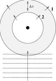
As is set up, a plane-wave of monochromatic radiation of $U^{(1)}(1)$ gauge field is incident on a free, massive W-boson of charge $Q$ and mass $M_{\rm W}$. The W-boson will be accelerated and emit radiation and, if the energy of the incident radiation is low enough compared to the mass $M$, the emitted radiation will have the same frequency as the incident radiation. The whole process then can be described by conventional Thomson scattering process, for which the W-boson is treated as a point-particle. As the W-boson is charged under $H$, the emitted radiation will consist of both $U^{(1)}(1)$ and $U^{(2)}(1)$ gauge fields field. In terms of the D3-branes, this means that both D3-branes will be excited by dipole oscillation of the stretched open string (interpreted as the massive W-boson) after the incident $U^{(1)}(1)$ radiation on the first D3-brane scatters off it, as depicted in figure 1.

Figure 1: Thompson scattering of brane wave off a W-boson. The incident $U^{(1)}(1)$ brane wave, whose wave front is denoted by dashed lines, is scattered off a point-like massive W-boson at rest. The scattered spherical brane waves of both $U^{(1)}(1)$ and $U^{(2)}(1)$ gauge groups, labelled as 1,2, are emitted instantly and simultaneously.

2.1.1 Scattering Equation of Motion

We will study dynamics of a massive W-boson, located at ${\bf X}(t)$, interacting with gauge fields of the gauge group $H$. From the D3-brane point of view, the W-boson is realized by an open F-string stretched between the two D3-branes. Denote spatial position (on the two D3-branes) of its endpoints as ${\bf X}_{1,2}(t)$. In the limit the W-boson is treated as a point-particle, the position of the W-boson ${\bf X}(t)$ ought to coincide with the two endpoint positions, ${\bf X}_{1,2}(t)$ all the time. Consider an incident plane-wave radiation of the $U^{(1)}(1)$ gauge field, whose wave vector and frequency are denoted by $\bf k$ and $\omega$, respectively. As the W-boson is charged with charge $(Q,-Q)$ under $H$, electric field of the incident radiation:

$${\cal E}({\bf x},t)={\bf E}^{(1)}(t)\,e^{i{\bf k}\cdot{\bf x}},\qquad{\bf E}^{(1)}(t)={\bf E}_{0}^{(1)}e^{-i\omega t},$$

according to the Lorentz force equation, will exert an instantaneous acceleration to the massive W-boson:

$$\ddot{\bf X}_{1}(t)=\ddot{\bf X}_{2}(t)={Q\over M_{\rm w}}{\bf E}^{(1)}(t)e^{i{\bf k}\cdot{\bf x}}.$$ (2.3)

Throughout this paper, we will consider the weak field-strength limit. In this case, the W-boson is in nonrelativistic motion and, at leading order, the spatial dependence of the electric field on the right-hand side of Eq.(2.3) may be ignored.

The Eq.(2.3) shows that the two ends, even though separated by a distance $\Delta r$, accelerates in an identical manner, viz. the stretched open F-string behaves like a rigid rod. It indicates that, should the open F-string be treated as a point-particle, super Yang-Mills theory on the D3-brane worldvolume would entail inevitably nonlocality over the distance scale $\Delta r$ in the direction perpendicular to the D3-brane. This is of course as it should be, in order for the perpendicular direction to be interpreted as color isospin direction.

2.1.2 Transmission Rate

To appreciate the significance of the Eq.(2.3), we will now calculate the rate of energy transmission $T$ from the first D3-brane to the second through the stretched open string. From Eq.(2.3), one can determined the instantaneous power $P(t)$ radiated into a polarization state $\bf\varepsilon$ by the W-boson is

$${dP\over d\Omega_{2}}={Q^{2}\over 4\pi c^{2}}|{\bf\epsilon}^{*}\cdot\ddot{\bf X}(t)|^{2}.$$ (2.4)

Averaging over a period $2\pi/\omega$, during which the charged particle moves a negligible fraction of one wavelength,

$$\Big{\langle}{dP\over d\Omega_{2}}\Big{\rangle}=c{{{\bf E}_{0}^{(1)}}^{2}\over 8\pi}\left({Q^{2}\over M_{\rm w}c^{2}}\right)^{2}|\epsilon^{*}\cdot\hat{\bf E}_{0}^{(1)}|^{2}.$$

The first factor $({{\bf E}_{0}^{(1)}}^{2}/8\pi)c$ is nothing but the incident energy flux, viz. the time-averaged Poynting vector for the plane wave. Hence, differential transmission rate for an unpolarized incident radiation is given by

$$\left({dT\over d\Omega_{2}}\right)_{\rm classical}=\left({Q^{2}\over M_{\rm w}c^{2}}\right)^{2}\cdot{1\over 2}\left(1+\cos^{2}\theta\right),$$ (2.5)

in which $\theta$ denotes the scattering angle in the laboratory frame. The total transmission rate $T$ obtained thereof is

$$T_{\rm classical}={8\pi\over 3}\left({Q^{2}\over M_{\rm w}c^{2}}\right)^{2}.$$

Characteristic feature of the classical Thomson scattering is that the cross-section is independent of the frequency of the scattered radiation. The result Eq.(2.5) is valid only at low frequency limit, $\omega\ll Mc^{2}$, for which the gauge field can be treated as a classical wave. As the energy of the incident radiation becomes larger and, especially, comparable to the W-boson mass, the scattering process should be treated quantum mechanically, viz. treating the radiation as photons. Treated in the Coulomb gauge for which the transition matrix element is identical to the classial amplitude, the modification is from the phase space factor and hence is purely kinematical. The result is

$$\left({dT\over d\Omega_{2}}\right)_{\rm quantum}=\left({Q^{2}\over M_{\rm w}c^{2}}\right)^{2}\left(\omega^{\prime}\over\omega\right)^{2}\cdot{1\over 2}(1+\cos^{2}\theta),$$

where the ratio of the outgoing to the incident frequency is given by the well-known Compton formula:

$${\omega^{\prime}\over\omega}=\left(1+2{\omega\over M_{\rm w}c^{2}}\sin^{2}{\theta\over 2}\right)^{-1}.$$

For low frequency limit, $\omega\ll M_{\rm w}c^{2}$, one easily obtains the transmission rate as

$$T_{\rm quantum}={8\pi\over 3}\left({Q^{2}\over M_{\rm w}c^{2}}\right)^{2}\left(1-2{\omega\over M_{\rm w}c^{2}}+\cdots\right).$$ (2.6)

Had we have considered a point-like limit of the magnetic monopole dual to the W-boson, represented by an open D-string stretched between the two D3-branes, the transmission rate would be essentially the same as above except that $M_{w}$ is to be replaced by the mass of the magnetic monopole $M_{m}$ and that the charge Q is interpreted as the dual magnetic charge [32].

To recapitulate, in the limit the W-boson is point-like, viz. the stretched F-string moves rigidly, the transmission of radiation energy from the first D3-brane to the second through W-boson is instantaneous and is a consequence of the standard field theory result, Eq.(2.3). Based on this fact, we conclude that the D3-brane worldvolume dynamics, if treated in terms of conventional super Yang-Mills theory and point-like W-bosons, would perceive nonlocality and acausality over a distance scale $\Delta r$ in the six-dimensional transverse space in $X$. From the super Yang-Mills theory point of view, this conclusion should be hardly surpring as the color isospin space is only an internal space and is not part of the four-dimensional spacetime (worldvolume of the D3-branes).

2.2 Scattering of Flat Brane-Wave by Charged Open String

From the underlying string theory point of view, nonlocality and acausality over the distance scale $\Delta r$ are extremely bizzare. The transverse to the D3-branes is six-dimensional subspace in $X$ and string theory ought to exhibit locality and causality, at least over a long distance limit. For example, energy transfer from the first D3-brane located at $r=r_{1}$ to the second at $r=r_{2}$ through the open string between them ought to take a causal time delay

$$\Delta t\equiv{1\over c}(r_{2}-r_{1})={\Delta r\over c},$$ (2.7)

as depicted in figure 2.

Figure 2: a stretched F- or D-string connecting two probe D3-branes in flat spacetime background. vibration of the stretched string causes retarded signal propagation between the two D3-branes only when the separation is bigger than the string scale.

Resolution of the puzzle is quite simple. As nonlocality and acausality has arisen from the point-particle limit of the W-boson, one expects that locality and causality will become transparent in the opposite limit, viz. the W-boson (realized as an open string stretched between the two D3-branes) is treated as a full-pledged string. This turns out correct and means that one will now need to study the Thomson scattering of the incident $U^{(1)}(1)$ radiation off a string-like W-boson. In fact, in this section, we will find that the W-boson dynamics is drastically modified from that in the point-particle limit and that the modified dynamics is precisely what allows to restore locality and causality of $X$.

2.2.1 Scattering Equations of Motion

Consider again the Thomson scattering of the $U^{(1)}(1)$ field radiation off the W-boson, but now in the limit the W-boson is treated as a full-fledged open string. Dynamics of the string is governed by Type IIB Green-Schwarz action, supplemented by an appropriate boundary action for the open string attached to the D3-branes. In Nambu-Goto formulation, which is sufficient for the Thomson scattering process, the action is constructed in Appendix A. After fixing the $\kappa$-symmetry in a gauge compatible with the boundary conditions and worldsheet reparametrization symmetries in static gauge, whose steps are explained in detail in Appendix A, one finds that the action for the string transverse coordinates ${\bf X}(r,t)$ is reduced to the form:

$$I_{\rm string} = \int dt\left[-M_{\rm w}+{T\over 2}\left({1\over c^{2}}\left(\partial_{t}{\bf X}\right)^{2}-\left(\partial_{r}{\bf X}\right)^{2}\right)+\cdots\cdots\right]$$

$$+ \sum_{\rm I=1,2}\int dt\,Q_{\rm I}\left[A_{0}^{\rm(I)}({\bf r},t)+{1\over c}\dot{\bf X}_{\rm I}\cdot{\bf A}^{\rm(I)}({\bf r},t)\right]_{r={\bf X}_{\rm I}(t)},\qquad(Q_{1}=-Q_{2}=\pm 1).$$

The first term in the expansion represents the static mass of the string, $T\Delta r$, which equals to the W-boson mass, $M_{\rm w}$ (see Eq.(2.2)). Consider, as posed above, Thomson scattering of a low-energy, monochromatic plane-wave of the $U^{(1)}(1)$ gauge field off the string endpoints. The boundary condition of the string coordinates ${\bf X}(t,r)$ is given by

$$T\partial_{r}{\bf X}(t,r)\Big{|}_{r=r_{1}} = Q{\bf E}^{\rm(1)}(t)$$

$$T\partial_{r}{\bf X}(t,r)\Big{|}_{r=r_{2}} = 0\,\,\,.$$ (2.9)

According to the first boundary condition, the string endpoint ${\bf X}_{1}(t)$ (on the first D3-brane) will undergo a dipole oscillation and generate a pulse that will propagate subsequently along the string. The pulse may be decomposed into spectral components

$${\bf X}(t,r)=\int{d\omega\over 2\pi}\left[\,\,{\bf a}(\omega)\,e^{-i\omega(t-r/c)}\,\,+\,\,\tilde{\bf a}(\omega)e^{-i\omega(t+r/c)}\,\,\right].$$ (2.10)

The spectral amplitudes ${\bf a}(\omega),\tilde{\bf a}(\omega)$ are determined uniquely by the Thomson scattering boundary condition Eq.(2.9):

$${\bf a}(\omega)\,\,=\,\,\tilde{\bf a}^{*}(\omega)\,\,=\,\,{Q{\bf E}_{0}^{(1)}\over 2\omega T}\left(\cot\omega\Delta t-i\right).$$ (2.11)

From Eqs.(2.10, 2.11), one immediately obtains an equation of motion for the string endpoint ${\bf X}_{1}(t)$ on the first D3-brane:

$$M_{\rm w}\left({\tanh\Delta t\partial_{t}\over\Delta t\partial_{t}}\right)\ddot{\bf X}_{1}(t)\,\,=\,\,Q{\bf E}^{(1)}(t).$$ (2.12)

One first finds that the inertia mass of the open string equals to the static mass, $M_{\rm w}$, as is dictated by the underlying Lorentz invariance. Compared to the point-particle limit of the W-boson, Eq.(2.3), equation of motion of the endpoint ${\bf X}_{1}(t)$ is changed to the one involving a kernel of infinite-order time derivatives. As will be shown in section 2.3, the extra kernel, which has originated from taking into account of the string oscillations, is what enables low-energy dynamics of the D3-brane worldvolume to reproduce locality and causality of the ambient spacetime $X$. For now, note that, due to the kernel, one may interpret the endpoint ${\bf X}_{1}(t)$ to behave heavier than the point-like W-boson mass $M_{\rm w}$.

What about the dynamics of the second endpoint ${\bf X}_{2}(t)$ attached to the second D3-brane? For point-particle limit of the W-boson, we have seen that the two endpoints behaves identically, see Eq.(2.3). What one now finds, however, is that the dynamics of the second endpoint is governed by a different equation of motion:

$$M_{\rm w}\left({\sinh\Delta t\partial_{t}\over\Delta t\partial_{t}}\right)\ddot{\bf X}_{2}(t)\,\,=\,\,Q{\bf E}^{(1)}(t).$$ (2.13)

Comparison with Eq.(2.12) shows that the infinite-order kernel associated with the second endpoint is different from that of the first one. In particular, the kernel lets us to interpret that the seocond endpoint ${\bf X}_{2}(t)$ behaves lighter than the point-like W-boson mass $M_{\rm w}$.

The Eqs.(2.12, 2.13) constitute defining equations for the Thompson scattering off the open F-string. Compared to the Thomson scattering off the massive W-boson, new effects have entered through D3-brane-separation-dependent (see Eq.(2.7)), infinite-order kernels. As the two endpoints obey different equations of motion, at any moment, one would expect that ${\bf X}_{1}(t)\neq{\bf X}_{2}(t)$. Therefore, from the super Yang-Mills theory perspective, it suggests to view the W-boson more naturally as a sort of an extended, bi-local object.

2.2.2 Transmission Rate Across Open String

Following the same steps as in section 2.1.2, it is straightforward to calculate the transmission rate $T$ (defined earlier in section 2.1.2) from the new equation of motion, Eq.(2.13) of the string endpoint on the second D3-brane.

Actually, one will need to take into account of another important corrections to the transmission rate: virtual W-boson pair and radiation reactive force effects. They are entirely of field-theoretic origin and have nothing to do with string oscillations. Because of these effects, in field theory treatment, the W-boson might be viewed roughly as a particle with an effective size set by the W-boson Compton wavelength. Heuristically, the effects may be understood as follows [33]. Low-energy dynamics of a single W-boson may be described by taking a non-relativistic limit of the W-boson gauge field $W_{\mu}$:

$$W_{0} = {1\over\sqrt{2M_{\rm w}}}{i\over M_{\rm w}c}e^{-iM_{\rm w}c^{2}t}\,{\bf D}\cdot{\bf\Phi}({\bf r},t)$$

$${\bf W} = {1\over\sqrt{2M_{\rm w}}}e^{-iM_{\rm w}c^{2}t}{\bf\Phi}({\bf r},t),$$ (2.14)

in which charge-conjugate, anti-particle part is suppressed. Expanding the super Yang-Mills Lagrangian in the non-relativistic limit, one finds

$${\cal L}_{\rm SYM}=-{1\over 4}F^{\mu\nu}F_{\mu\nu}+i{\bf\Phi}^{\dagger}\cdot D_{t}{\bf\Phi}+{1\over 2M_{\rm w}}{\bf\Phi}^{\dagger}\cdot{\bf D}^{2}{\bf\Phi}-i{Q\over M_{\rm w}c}{\bf B}\cdot{\bf\Phi}^{\dagger}\times{\bf\Phi}+\cdots.$$ (2.15)

This can be reduced further to a single particle Lagrangian of the W-boson:

$$L_{\rm w} = {1\over 2}m_{\rm w}\dot{\bf X}\cdot\dot{\bf X}+Q\left(A_{0}+{1\over c}\dot{\bf X}\cdot{\bf A}\right)+{\bf S}\cdot{\bf B}+\cdots$$ (2.16)

$$- \int d{\bf r}\left({1\over 4}F^{\mu\nu}F_{\mu\nu}\right).$$

Here, parts containing classical spin dynamics and interaction with Higgs field are suppressed for brevity. Following Abraham-Lorentz-type approach [16], it is straightforward to derive an effective equation of motion that takes into account of radiative reaction force. One obtains

$$M_{\rm w}\left(1-{Q^{2}\over 4\pi}{\partial_{t}\over M_{\rm w}}+\cdots\right)\ddot{\bf X}(t)=Q{\bf E}_{0}(t).$$ (2.17)

If one takes into account of virtual W-boson pair corrections, one also obtains a term similar to the second on the left-hand side. At low frequency, the second term is suppressed compared to the first by ${\cal O}(\omega/M_{\rm w})$ and hence, according to Eq.(2.4), gives rise to ${\cal O}(\omega^{2}/M^{2}_{\rm w})$ correction to the transmission rate.

Taking into account of the above effects, one obtains the transmission rate for F-string as:

$$T_{\rm F-string}={2\pi\over 3}\left({Q^{2}\over M_{\rm w}c^{2}}\right)^{2}\left(1-2{\omega\over M_{\rm w}c^{2}}+\cdots\right)\cdot\left(1-\left({\omega\over M_{\rm w}c^{2}}\right)^{2}+\cdots\right)\cdot\left[{\omega\Delta t\over\sin\omega\Delta t}\right]^{2}.$$ (2.18)

The first two brackets represent the result derived from the limit the W-boson is treated as a point-particle. The third bracket is the correction due to virtual W-boson and radiation reactive force effect estimated above. The last bracket comes from the string oscillation effects, viz. from the fact that the massive W-boson is actually a stretched open string.

It is instructive to consider the transmission rate for, instead of a F-string, a D-string is stretched between the two D3-branes. From super Yang-Mills point of view, the open D-string corresponds to a magnetic monopole dual to W-boson. In this case, scattering of the brane wave takes place from interaction of the open D-string with magnetic component of the radiation field. The corresponding transmission rate is obtained straighforwardly:

$$T_{\rm D-string}={2\pi\over 3}\left({Q^{2}\over M_{\rm m}c^{2}}\right)^{2}\left(1-2{\omega\over M_{\rm m}c^{2}}+\cdots\right)\cdot\left(1-\left({\omega\over M_{\rm w}c^{2}}\right)^{2}+\cdots\right)\cdot\left[{\omega\Delta t\over\sin\omega\Delta t}\right]^{2},$$ (2.19)

where $Q$ should now be interpreted as magnetic charge of the dual W-boson. One again finds that, apart from the kinematical, Compton scattering correction, corrections of ${\cal O}(\omega^{2}/M_{\rm w}^{2})$ arise from the classical finite-size of the magnetic monopole, set by the Compton wavelength of the W-boson, and radiation reactive force effects [33].

We emphasize that, for both W-boson and its dual magnetic monopole, the correction due to finite-size and radiation reactive force effects is set by the W-boson mass, $M_{\rm w}$. Given that it is the only low-energy threshold scale in the system at weak coupling limit, the fact that the correction for both W-boson and magnetic monopole is governed by the same low-energy scale should not be surprising .

2.3 Locality and Causality in Flat Spacetime

Having analyzed transmission of brane waves across open string at two different limits, we will now study causality and locality of ambient spacetime as seen by super Yang-Mills theory.

2.3.1 Retarded Dynamics of String Endpoints

We have already seen from Eq.(2.3) that, in the limit the massive W-boson behaves like a point particle, the string endpoint on the second D3-brane, despite being separated by a distance $\Delta r$, responds to the incident brane wave localized on the first D3-brane instantaneously. As such, scattered brane wave will come out of both isospin components of $T_{3}$ (labelling the two D3-branes) simultaneously, with no apparent causal time-delay between the two isospin components. See figure 1. Indeed, the transmission rate, Eq.(2.6), is exactly the same as the classic Thomson scattering cross-section. As a result, one will conclude that any super Yang-Mills theory with pointlike W-bosons will not be able to encode causality and locality of ambient spacetime.

In the opposite limit where the W-boson is a full-fledged oscillating string, Eq.(2.10) shows that a pulse propagating along the string is described by characteristic functions of the form $f(t\pm r/c)$. Clearly, it will take a causal time delay $\Delta t$, Eq.(2.7), for the pulse, induced by the incident brane wave on the first D3-brane, to reach the second D3-brane. To appreciate the causal time-delay more transparently, let us rewrite the equation of motion of second string endpoint, Eq.(2.13), into an integral equation form:

$$M_{\rm w}\ddot{\bf X}_{2}(t)=\int dt^{\prime}\,\,\Theta(t-t^{\prime})\bigg{\langle}t\bigg{|}{\Delta t\partial_{t}\over\sinh\Delta t\partial_{t}}\bigg{|}t^{\prime}\bigg{\rangle}\cdot Q{\bf E}^{(1)}(t^{\prime}),$$ (2.20)

where the Heaviside step function follows from convergence requirement, as is usual in any nonrelativistic dynamics. The integral kernel shows manifestly that the time-delay between Note that the integral kernel has infinitely many poles but no zeros.

The equation of motion, Eq.(2.13), can be put into an equivalent to Eq.(2.20), but even more suggestive form by observing the fact that the infinite-order kernel is in fact a difference operator:

$${\bf X}_{2}(t+\Delta t)-{\bf X}_{2}(t-\Delta t)=2\Delta t\int^{t}dt^{\prime}\,Q{\bf E}^{(1)}(t^{\prime}),$$ (2.21)

displaying manifestly that it takes causal time-delay $\Delta t$ for the brane wave on the first D3-brane, ${\bf E}^{(1)}$, to arrive at the second. The fact that the time-delay is exactly $\Delta t$ as estimated from the geometric distance between the two D3-branes, Eq.(2.7) also implies that the boundary interactions between F-string and D3-branes are local.

While encoding causality and locality quite successfully, the massive W-boson in this limit is far from the point-like object one casually take in Yang-Mills theory. Rather, the two endpoints ${\bf X}_{1,2}(t)$ of the open string evolves independently. Hence, projected on D3-brane worldvolume, the W-boson is now replaced by a sort of extended, bilocal object whose dynamics is captured by the equations of motion, Eqs.(2.12, 2.13).

2.3.2 Physical Thresholds: ‘Winding’ versus ‘Momentum’

As is evident from the transmission rates, Eqs.(2.18, 2.19), frequency-dependent corrections are characterized by two distinct physical threshold scales inherent to the problem. The first is set by the W-boson mass, $M_{\rm w}=T\Delta r$, defining a physical threshold (of field theoretic origin) above which description in terms of abelian gauge theory with gauge group $H$ breaks down. The second is set by energy gap of string oscillation, $1/\Delta t=c/\Delta r$, above which a point-particle description of the W-boson breaks down. Being proportional to $\Delta r$ and inversely to $\Delta r$, respectively, we shall be referring the first threshold as ‘winding threshold’ $\Lambda_{\rm w}$ and the second as ‘momentum threshold’, $\Lambda_{\rm m}$:

$$\Lambda_{\rm w}=M_{\rm w}=T\Delta r,\qquad\quad\Lambda_{\rm m}={1\over\Delta t}={\hbar c\over\Delta r}.$$ (2.22)

As there are two distinct physical thresholds, depending on which one sets the lower scale, low-energy dynamics of the super Yang-Mills theory will become quite different. As the winding and momentum thresholds depend on the spatial separation $\Delta r$ inversely, the two will competes each other as $\Delta r$ is varied. The competition may be summarized into a form of string uncertainty relation ($T\equiv 1/\ell_{s}^{2}$)

$$\Lambda_{\rm w}\Lambda_{\rm m}\quad\approx\quad{\cal O}\left({\hbar c\over\ell_{s}^{2}}\right).$$ (2.23)

Note that the right-hand-side, a combination of fundamental constants only, depends crucially on the string scale, $\ell_{s}$. It implies that any effects related to causal retardation, which arises from oscillation threshold corrections, will inevitably depends on it, as $\partial/\Lambda_{\rm m}\approx\ell_{s}^{2}M_{\rm w}\partial$. This explains the observation of Douglas and Taylor [23] on $F^{4}$ interaction between brane waves with nonzero momentum. As $M_{\rm w}\propto\Delta r\propto\Delta t$, one again finds that successive power corrections in oscillation threshold are nothing but the retardation time expansion of Eq.(2.20).

Hence, if $\Lambda_{\rm w}\ll\Lambda_{\rm m}$, threshold effects to low-energy processes dominated by the ‘winding threshold’. As string oscillation excitations are completely irrelevant, the stretched open string behaves literally like a rigid-rod, to which the D3-branes serve as a pair of guiderail. Behaving as a rigid body, the open string may be treated as a point-particle, massive W-boson. As the condition

$$\Lambda_{\rm w}\ll\Lambda_{\rm m}\quad\rightarrow\quad\Delta r\ll\ell_{s},$$ (2.24)

one find that the limit in which the D3-brane worldvolume dynamics is best approximated by super Yang-Mills theory, either in conventional (renormalizable dimension-four operators) or Dirac-Born-Infeld form, is when the D3-brane separation is over a sub-stringy scale, reproducing well-known result [26].

Exactly the same condition applies if the stretched F-string is replaced by a D-string. An open D-string stretched between two D3-branes is casually identified with a magnetic monopole dual to the massive W-boson. Its classical size is set by the Compton wavelength of the massive W-boson $M_{\rm w}=T\Delta r$ and defines the field theoretic, winding threshold scale $\Lambda_{\rm w}$. Requirement that this scale is much less than the oscillation threshold scale $\Lambda_{\rm m}$, which is the same for both F- and D-string, again set the condition, Eq.(2.24).

3 Dynamical Aspect of Energy-Size Relation

An important feature of the AdS/CFT correspondence is holographic relation between the radial position, ‘energy scale’, in anti-de Sitter spacetime and ‘size’ in super Yang-Mills theory. As this relation will be playing a crucial role for foregoing discusssions, we will be studying first dynamical aspect of the relation. More specifically, for heavy quark and meson studied in [30, 31], we will estimate causal time-delay for a pulse generated by a quark either along the string in anti-de Sitter spacetime or in Minkowski spacetime, using the harmonic fluctuation Lagrangian of the string studied previously [29, 30, 34]. We will find that, after utilizing the holographic energy-size relation, the two estimates agree perfectly with each other.

A charged probe necessarily accompany long-range Coulomb field, so it will be necessary to control the field configuration in the infrared. A convenient way is to move into the Coulomb branch, viz. separating some of the D3-branes and then study a state charged under the gauge group of the separated D3-branes. The $N$ coincident D3-branes sitting at the conformal point then generates the anti-de Sitter spacetime as a near-horizon geometry [1]

$$ds^{2}=\ell_{s}^{2}\left[\,{U^{2}\over g_{\rm eff}}\left(-{1\over c^{2}}dt^{2}+d{\bf x}_{|\hskip-0.85355pt|}^{2}\right)+g_{\rm eff}{dU^{2}\over U^{2}}+g_{\rm eff}d\Omega_{5}^{2}\,\right],\qquad\quad(U\equiv Tr,\,\,T=1/\ell^{2}_{s}).$$ (3.25)

In this coordinate, the energy-scale holographic relation asserts that the scale position $U$ in the anti-de Sitter spacetime is related directly to the scale size $R$ in the super Yang-Mills theory:

$$R\quad=\quad{g_{\rm eff}\over U}.$$ (3.26)

This relation has been first derived from evaluation of the Wilson loop [30, 31] and later extended to more general contexts [7].

3.1 Holography of Heavy Quark Dynamics

Consider a heavy quark of large-N super Yang-Mills theory at zero temperature. We will separate a single D3-brane to the Coulomb branch and consider a quark coupled to it. Denote the location of the displaced probe D3-brane as $U_{*}$. Then, a heavy quark (monopole) of the super Yang-Mills theory is realized by a macroscopic F- (D-) string ending on the displaced D3-brane at $U=U_{*}$ and stretched outward along the $U$-direction. Dynamics of the macroscopic string may be studied using Nambu-Goto action in the anti-de Sitter spacetime, Eq.(3.25). Taking static gauge $(\tau,\sigma)=(t,U)$ and expanding string transverse coordinates $({\bf X}_{|\hskip-0.85355pt|},\Omega_{5})$ up to harmonic fluctuations, one finds [30]

$$L_{\rm NG}=-\int_{U_{*}}^{\infty}dU+\int_{U_{*}}^{\infty}dU{\cal L}^{(2)}+L_{\rm boundary}$$ (3.27)

where

$${\cal L}^{(2)}={1\over 2}\left[\left({1\over c^{2}}{\dot{\bf X}}_{|\hskip-0.85355pt|}^{2}-{U^{4}\over g^{2}_{\rm eff}}{{\bf X}^{\prime}_{|\hskip-0.85355pt|}}^{2}\right)+U^{2}\left({g^{2}_{\rm eff}\over U^{4}}{1\over c^{2}}\dot{\Omega}_{5}^{2}-{\Omega^{\prime}_{5}}^{2}\right)\right]+\cdots$$ (3.28)

and $L_{\rm boundary}$ specifies boundary conditions at $U=U_{*}$.

Let us begin with static properties of the macroscopic string. The first term in Eq.(3.27) represent the static mass of the string

$$M_{\rm string}(U_{*})=\int_{U_{*}}^{\Lambda_{\rm UV}}dU,\hskip 85.35826pt\Lambda_{UV}\rightarrow\infty.$$ (3.29)

The static mass diverges as the cutoff $\Lambda_{\rm UV}$ is removed. As shown first in [30, 31] and discussed further [7, 10], this is nothing but anti-de Sitter space manifestataion of divergent self-energy of a heavy quark. A physically meaningful, finite quantity would be a residual static mass between strings ending on different locations of $U_{*}$, which we may define as

$$\Delta M_{\rm string}(U_{*})\equiv\int_{0}^{U_{*}}dU\,{dM_{\rm string}\over dU}=U_{*}.$$ (3.30)

Figure 3: Coulomb branch view gauge field generated by a test quark (monopole)

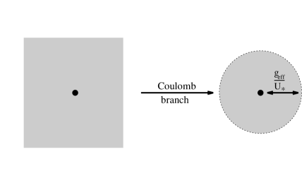
Using the scale-size relation Eq.(3.26), one then finds immediately that $\Delta M_{\rm string}(U_{*})=g_{\rm eff}/R_{*}$ corresponds to the Coulomb field energy measured at radius $R_{*}$. To understand this scale better, let us interpret the macroscopic string from the super Yang-Mills theory side. At the origin of the Coulomb branch (viz. $U_{*}=0$), the macroscopic string creates not only a heavy quark (transforming as the defining representation of $SU(N)$) itself but also long-range color Coulomb field around it, as depicted in the left of Figure 3. Away from the origin of the Coulomb branch, one might expects that the long-range Coulomb field is cut-off at the Compton wavelength $U_{*}^{-1}$ of the massive gauge bosons . However, as pointed out in [30, 31], the strong ‘t Hooft coupling dynamics cuts off the long-range field at a larger scale, $g_{\rm eff}U^{-1}_{*}$. Thus, we find that $\Delta M_{\rm string}$ is nothing but the ‘field energy’, the energy associated with Coulomb field outside radius $R_{*}=g_{\rm eff}/U_{*}$ in the Yang-Mills theory. Summarizing, static property (such as static mass) of the macroscopic string is determined by the quantity $\int dU$.

Figure 4: string attached to a probe D3-brane in anti-de Sitter space

What about dynamical properties? Consider exciting a low-energy pulse at the outer end of the string, as depicted in Figure 4.. The pulse will then propagate at the speed of light (which has been explicitly checked in [30]) along the string toward $U_{*}$. According to the energy-size relation, in super Yang-Mills theory, the pulse travelling along the string is mapped, in super Yang-Mills theory, to a spherical brane wave generated at the position of the heavy quark and then propagating outward. For the spherical wave to propagate over a radial size $R_{*}$, it will take Yang-Mills time:

$$(\Delta t)_{\rm YM}={1\over c}R_{*}.$$ (3.31)

If causality is implied by the holographic energy-size relation, then the time-delay for the pulse propagation along the string should be the same as that for the spherical brane wave propagating outward. Let us check this explicitly. The string pulse propagates along the string, viz. a null geodesic in $(U,t)$ subspace:

$${U^{2}\over g_{\rm eff}}\Delta t^{2}={g_{\rm eff}\over U^{2}}\Delta U^{2}.$$ (3.32)

Thus, measured from anti-de Sitter spacetime in Yang-Mills time unit, causal time-delay for the pulse to travel from $U=\infty$ to $U=U_{*}$ along the string is given by

$$\left(\Delta t\right)_{\rm AdS}={1\over c}g_{\rm eff}\int_{U_{*}}^{\infty}{dU\over U^{2}}={1\over c}{g_{\rm eff}\over U_{*}}.$$ (3.33)

Remarkably, the holographic energy-size relation, Eq.(3.26), permits the causal time delay in the anti-de Sitter spacetime agrees exactly with that along the boundary!

3.2 Holography of Heavy Quark Dynamics at Finite Temperature

Consider next the super Yang-Mills theory at nonzero temperature. The near-horizon geometry of near extremal D3-branes is described by the anti-de Sitter-Schwarzschild spacetime, whose $(t,U)$ subspace is given by:

$$ds^{2}=\ell_{s}^{2}\left[\,-{1\over c^{2}}\left(1-{U_{0}^{4}\over U^{4}}\right){U^{2}\over g_{\rm eff}}dt^{2}+{g_{\rm eff}\over U^{2}}\left(1-{U_{0}^{4}\over U^{4}}\right)^{-1}dU^{2}\,\right].$$ (3.34)

From Nambu-Goto Lagrangian, one again finds that the static mass of the string is given by

$$M=\int_{U_{0}}^{\infty}dU,$$ (3.35)

the same as the value at zero temperature.

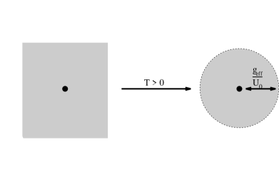
Let us introduce a heavy quark to the Yang-Mills theory at finite temperature. The quark is described by a macroscopic F-string stretched along $U$-direction [34, 35], as depicted in Figure 5. In the present case, the string terminates at the Schwarzschild horizon, $U=U_{0}$, where it will dissipate the F-string flux into the inner horizon region.

Figure 5: Pulse propagation along semi-infinte string in anti-de Sitter Schwarzschild spacetime.

This phenomenon has a direct counterpart in super Yang-Mills theory. At zero temperature, Coulomb field of the static quark extends everywhere, as depicted at the left in Figure 4. At finite temperature, however, the Coulomb field becomes Debye-screened and is expected to extend to the scale of Debye wavelength $U_{0}^{-1}=(g_{\rm eff}T)^{-1}$. Using the holographic energy-size relation, one finds that the Coulomb field is cut off at a larger scale $g_{\rm eff}U_{0}^{-1}$, again due to strong ‘t Hooft coupling dynamics. See Figure 6.

Figure 6: aerial view of an isolated quark in super Yang-Mills theory at finite temperature

In fact, by demanding causality, one can understand the fact that string must end at $U=U_{0}$. Consider a weak pulse injected at $U=\infty$ and propagating inward. The time-delay for the pulse to reach the position $U(U_{0}\leq U\leq\infty)$ is easily estimated:

$$(\Delta t)_{\rm AdS}={g_{\rm eff}\over U_{0}}\int_{0}^{U_{0}/U}{dx\over 1-x^{4}}.$$ (3.36)

The time-delay diverges logarithmically as $U\rightarrow U_{0}$. So, evolved in terms of Yang-Mills theory time, which is an asymptotic observer’s time in the anti-de Sitter spacetime, the super Yang-Mills theory covers spacetime region only outside the horizon. If a different global time is chosen as an evolution operator, then the string might be able to enter inside the horizon. In this case, howeve, the string would not be in a static configuration [9]

At finite temperature, the scale $R_{0}=g_{\rm eff}U_{0}^{-1}$ corresponds to a physical threshold scale in Yang-Mills theory. At weak ‘t Hooft coupling limit, Matsubara mass scale associated with dimensionally reduced fermions (satisfying anti-periodic boundary condition around Euclidean time) is ${\cal O}(T)$, which equals to $U_{0}/g_{\rm eff}$. If this observation somehow holds also for super Yang-Mills theory at zero temperature, then we are prompted to expect that the scale $R_{*}\equiv g_{\rm eff}U_{*}^{-1}$ actually corresponds to a new physical threshold scale. Recall that this scale is not a threshold of an elementary excitations as the Compton wavelength of massive gauge bosons $U^{-1}_{*}$. Nevertheless, the fact that the scale $R_{*}$ is $g_{\rm eff}$ times Compton wavelength of massive gauge bosons is tantalizingly similar to the observation of Shenker made in a different context [36].

3.3 Holography of Heavy Meson Dynamics

Figure 7: A pulse propagatiing along the Wilson loop in anti-de Sitter spacetime.

A more intricate bulk probe is the macroscopic string configuration corresponding to the heavy meson [30, 31]. In the static gauge, the string configuration is specified by a first-integral of motion:

$$G^{2}U^{\prime 2}+G={g^{2}_{\rm eff}\over U_{*}^{4}}.$$ (3.37)

Again, consider a pulse propagating along the string, $U=U(\sigma)$. The time delay for the pulse to travel between the quark and anti-quark (both ‘located’ at $U=\infty$) along the string is again calculated straightforwardly by solving string equation of motion along the null geodesic:

$$\sqrt{G}dU^{2}={1\over\sqrt{G}}\left(-dt^{2}+d\sigma^{2}\right)\,.$$ (3.38)

This yields

$$(\Delta t)_{\rm AdS}=\int_{-d/2}^{+d/2}d\sigma\sqrt{GU^{\prime 2}+1}.$$ (3.39)

Using Eq.(3.37), one finds immediately that

$$(\Delta t)_{\rm AdS} = 2{g_{\rm eff}\over U_{*}^{2}}\int_{U_{*}}^{\infty}dU{1\over\sqrt{U^{4}/U^{4}_{*}-1}}$$ (3.40)

$$= {2\sqrt{\pi}\Gamma(5/4)\over\Gamma(3/4)}{g_{\rm eff}\over U_{*}}.$$

From the super Yang-Mills theory side, natural scale of the meson is the inter-quark distance $d$. Hence, one expects that

$$\left(\Delta t\right)_{\rm YM}=A{1\over c}d,$$ (3.41)

where $A$ is a ${\cal O}(1)$ numerical coefficient, which should reflect the details of the dipole field configuration produced by the quark-antiquark pair at strong ‘t Hooft coupling limit. For mesons, precise form of the holographic energy-size relation has been derived [30, 31]:

$${d\over 2}={{\sqrt{\pi}}\Gamma(3/4)\over\Gamma(1/4)}{g_{\rm eff}\over U_{*}},$$ (3.42)

Hence, equating $\Delta t$ of anti-de Sitter spacetime with that of Yang-Mills theory, one finds that

$$A={\Gamma(5/4)\Gamma(1/4)\over\Gamma^{2}(3/4)}=2.188...$$ (3.43)

Figure 8: Aerial view of the quark anti-quark pair and dipole field configuration produced thereof.

The numerical factor, $A=2.188...$, associated with the dipole electric field configuration of the quark antiquark pair as depicted in figure 8, may be viewed as a prediction for the strong ‘t Hooft coupling dynamics from anti-de Sitter supergravity.

4 Causality and Locality in Anti-de Sitter Spacetime

Having understood dynamical aspect of the energy-size relation better, we will now revisit the Thomson scattering of brane waves by an open string and consequent implications to the issue of causality and locality, but now all in anti-de Sitter spacetime.

We will be showing that ‘momentum’ threshold of the open string stays always below the ‘winding’ threshold everywhere in the anti-de Sitter spacetime. Moreover, quite importantly, both thresholds does not depend on the string scale, $\ell_{s}$. Thus, in sharp contrast to the flat spacetime situation, we will be able to encode causality and locality of semi-classical supergravity in anti-de Sitter spacetime in terms of large-$N$ super Yang-Mills theory, at least in the strong ‘t Hooft coupling limit. The resulting super Yang-Mills theory is not the standard one, however. At at generic point of the Coulomb branch moduli space, we will be finding that infinite tower of long supermultiplet operators should be included to be able to encode the bulk causality and locality. Once again, this conclusion is drawn from the fact that W-bosons are more suitably described by a sort of extended, bilocal objects.

4.1 D3-Branes in the Coulomb Branch

The anti-de Sitter spacetime is generated as near-horizon geometry of infinitely many $(N\rightarrow\infty)$ D3-branes when they become coincident one another. Therefore, to explore causality and locality of the anti-de Sitter spacetime, from the viewpoint of super Yang-Mills theory, one will need to examine low-energy dynamics near the origin of the Coulomb branch moduli space, where the Higgs expectation values are interpreted as positions of individual D3-branes in anti-de Sitter spacetime [1, 23].

As in flat spacetime, we will be considering two D3-branes out of $N$ coincident oneses are located at positions $U_{1},U_{2}$, respectively, and a macroscopic open string stretched between them. We will again excite the displaced probe D3-branes with low-energy brane waves and study Thomson scattering off the open string. The configuration corresponds to the following sequential symmetry breaking:

$$SU(N)\rightarrow G=S\left[U(N-2)\times U(2)\right]\rightarrow H=S\left[U(N-2)\times(U(1)\times U(1))\right].$$ (4.44)

From super Yang-Mills theory perspectives, this appears quite a complicated problem, as the excitation of, say, first D3-brane will reach to the second D3-brane not only through the prescribed open string stretched between them but also indirectly through the coincident $(N-2)$ D3-branes, with which the two D3-branes interact. At the least, because the number of possible transmission channels through the ‘background’ $(N-2)$ D3-branes is humongous, ${\cal O}(N^{2})$, one might be tempted to conclude that, in the super Yang-Mills theory, brane wave transmission is not mediated through the massive W-bosons but by some sort of complicated large-$N$, strong ‘t Hooft coupling dynamics.

This, however, shouldn’t be a problem. The point is that interaction between the probe Yang-Mills theory with gauge group $U(2)$ or $U(1)\times U(1)$ and that of conformal sector with gauge group $SU(N-2)$ are controlled by the mass scales, $U_{1,2}$. Taking $\Delta U=|U_{1}-U_{2}|$ much lighter and $g_{\rm st}$ sufficiently small, dynamics of the two probe D3-brane sector can be studied in a controllable manner. Thus, starting from the super Yang-Mills theory with gauge group $G$, we will be integrating out over the Higgs branch, viz. open strings transforming in $({\bf N-2},\overline{\bf 2})$ and its complex-conjugate representations. In the $g_{\rm st}\rightarrow 0$, $N\rightarrow\infty$ and large ‘t Hooft coupling limit, the integration amounts to resummation of large-$N$ Feynman diagrams. As have argued in [1] (see also discussions in [23]), the result is to produce anti-de Sitter spacetime, inside which the two displaced probe D3-branes are localized.

Intuitively, the above assertion may be understood by observing that variance of positions of the $(N-2)$ coincident D3-branes and two displaced D3-branes are of order $(g_{\rm st}N)^{1/4}$ and $(g_{\rm st})^{1/4}$, respectively. That is, in the large-N limit, position of the two probe D3-branes is sharply localized inside the anti-de Sitter spacetime. It should also become clear that, even after adding a stretched open string between the two displaced D3-branes (associated with the symmetry breaking $G\rightarrow H$), integration over the Higgs branch yields essentially the same result, viz. dynamics of both the two probe D3-branes and the stretched open string between them will perceive the ambient background as anti-de Sitter spacetime.

Henceforth, at $g_{\rm st}\rightarrow 0$, $N\rightarrow\infty$ and strong ‘t Hooft coupling regime, we will be able to study causality and locality of the anti-de Sitter spacetime in a controllable manner by focusing only to low-energy excitations of massive W-bosons in ‘quantum corrected’ super Yang-Mills theory with symmetry breaking pattern $U(2)\rightarrow U(1)\times U(1)$.

4.2 Scattering of Brane Wave by Charged Open String

Dynamics of the open F-string stretched between the two D3-branes is governed by the Type IIB Green-Schwarz action in the anti-de Sitter spacetime. In Appendix B, for Nambu-Goto form of the action, details of gauge fixing of local $\kappa$- and reparametrization symmetries are explained. It turns out the gauge-fixing as well as analysis of string dynamics thereof become enormously simplified once one adopts a new coordinate, $R\equiv g_{\rm eff}/U$. According to the energy-size holography relation, Eq.(3.26), the new coordinate $R$ is seen nothing but the ‘size’ variable of super Yang-Mills theory. It is interesting that, in analyzing a ‘bulk’ process in anti-de Sitter spacetime, description in terms of a ‘boundary’ variable turns out more suited and efficient. Indeed, in terms of the ‘size’ coordinate $R$, the metric of the anti-de Sitter spacetime is given in Poincaré coordinates:

$$ds^{2}_{\rm AdS}={g_{\rm eff}\over R^{2}}\Big{[}-dt^{2}+d{\bf x}^{2}_{|\hskip-0.85355pt|}+dR^{2}+R^{2}d\Omega_{5}^{2}\Big{]}.\\$$

As elaborated in Appendix B, this coordinate choice leads the Green-Schwarz action to an almost identical form, after gauge fixing, to the one in flat spacetime, for both bosonic and fermions parts. Moreover, as has been observed in [30], harmonic dynamics of the open string turns out considerably simplied in the Poincaré coordinate system. After the gauge-fixing, the open string action is given by

$$I_{\rm string} = \int\!dt\,\left[-M_{\rm w}+{g_{\rm eff}\over 2}\int_{R_{1}}^{R_{2}}{dR\over R^{2}}\left({1\over c^{2}}(\partial_{t}{\bf X})^{2}-(\partial_{R}{\bf X})^{2}\right)+\cdots\right]$$ (4.45)

$$+ \sum_{\rm I=1,2}\int\!dt\,Q_{\rm I}\left[A_{0}^{\rm(I)}({\bf r},t)+{1\over c}\dot{\bf X}_{\rm I}(t)\cdot{\bf A}^{\rm(I)}({\bf r},t)\right]_{{\bf r}={\bf X}_{\rm I}(t)}.$$ (4.46)

Figure 9: a stretched F- or D-string connecting two probe D3-branes in the Coulomb branch. vibration of the stretched string causes retarded radiation between the two D3-branes.

First, one notes that static mass of the string as measured in anti-de Sitter spacetime, the first term in Eq.(4.45), $g_{\rm eff}\int dR/R^{2}$ equals to $(U_{2}-U_{1})$ in terms of the original ‘energy’ coordinate. Similar result holds also for an open D-string stretched between the two D3-branes. Hence,

$$M_{\rm w}=\Delta U,\quad\qquad M_{\rm m}={1\over g_{\rm st}}\Delta U.$$ (4.47)

Recalling that $\Delta U=T\Delta r$ (cf. Eq.(3.25)), one discovers that static mass of the string in anti-de Sitter spacetime is the same as that in flat spacetime. This is, from the super Yang-Mills theory perspective, as it should be. Both W-boson and dual magnetic monopole are BPS-saturated states and hence their masses are not renormalized as one interpolates from weak to strong ‘t Hooft coupling regime.

From Thomson scattering process in flat spacetime, we have observed that the static mass of the W-boson and the causal time-delay are governed by one and the same length scale, $\Delta r$, the separation between the two D3-branes. As the W-boson is a BPS state, one might have guessed that it will be the same in anti-de Sitter spacetime. After all, the distance between the two D3-branes is the only relevant length scale inherent in the problem. This expectation, however, turns out not quite right. We will be showing below that the causal time-delay is governed not by the scale $\Delta U$, but by

$$\Delta\tau\equiv{1\over c}\Delta R={1\over c}g_{\rm eff}\bigg{|}{1\over U_{1}}-{1\over U_{2}}\bigg{|}.$$ (4.48)

It is clear that $\Delta\tau$ has no simple functional relation to $\Delta U$, the scale that has set the W-boson mass for both flat and anti-de Sitter spacetime and the energy variance that the spacetime uncertainty relation [25] utilizes. In fact, the reason why $\Delta(g_{\rm eff}/U)$, not $\Delta U$, should be the relevant variable for the time-delay may be gleaned from the fact that $SO(4,2)$ invariant line element between two points $(t,U,{\bf x})_{1,2}$ is given by

$$\Delta s^{2}_{\rm AdS}=U_{1}U_{2}\left[-(t_{1}-t_{2})^{2}+g_{\rm eff}^{2}\left({1\over U_{1}}-{1\over U_{2}}\right)^{2}+({\bf x}_{1}-{\bf x}_{2})^{2}\right].$$ (4.49)

4.2.1 Scattering Equation of Motion

Consider excitation of a low-energy, monochromatic plane-wave of the $U^{(1)}(1)$ gauge field on the first D3-brane. As in flat spacetime, we will be studying Thomson scattering of the brane-wave off the open string. We have argued above that, in so far as $g_{\rm st}=g_{\rm YM}^{2}\rightarrow 0$, low-energy processes between the two probe D3-branes can be trusted. Actually, the Thomson scattering process depends on the combination of $g_{\rm YM}{\bf E}_{0}/M_{\rm w}$. Thus, even in the situation where $g_{\rm YM}$ itself may not be sufficiently small, the foregoing calculations will be completely controllable by taking the brane waves sufficiently weak.

In static gauge, the boundary condition of the transverse string coordinates ${\bf X}(t,R)$ is given by

$${g_{\rm eff}\over R^{2}}\partial_{R}{\bf X}(t,R)\bigg{|}_{R=R_{1}}\,\,\, = \,\,\,Q{\bf E}^{(1)}(t),$$

$${g_{\rm eff}\over R^{2}}\partial_{R}{\bf X}(t,R)\bigg{|}_{R=R_{2}}\,\,\, = \,\,\,0\,\,.$$

From Eq.(4.45), one finds that a weak pulse propagating along the string is given by

$${\bf X}(t,R)=\int{d\omega\over 2\pi}\left[\,{\bf a}(\omega)\,\left(1-i\omega{R\over c}\right)e^{-i\omega(t-R/c)}+\,\tilde{\bf a}(\omega)\,\left(1+i\omega{R\over c}\right)e^{-i\omega(t+R/c)}\,\right].$$ (4.51)

Again, the boundary condition, Eq.(LABEL:adsbc), fixes the spectral amplitudes ${\bf a}(\omega),\,\tilde{\bf a}(\omega)$ uniquely:

$${\bf a}(\omega)=\tilde{\bf a}^{*}(\omega)=\left({R_{1}/g_{\rm eff}\over\omega}\right)\left({Q{\bf E}_{0}^{(1)}\over\omega}\right){e^{-i\omega R_{2}/c}\over 2i\sin\omega\Delta\tau}.$$ (4.52)

Substituting Eq.(4.52) into Eq.(4.51), one obtains equation of motion for the string endpoint ${\bf X}_{1}(t)$ on the first D3-brane:

$$M_{\rm w}\left(1+{R_{1}\over R_{2}}\left({\Delta\tau\partial_{t}\over\tanh\Delta\tau\partial_{t}}-1\right)\right)^{-1}\ddot{\bf X}_{1}(t)\,\,\,=\,\,\,Q{\bf E}^{(1)}(t).$$ (4.53)

Comparison with the corresponding equation Eq.(2.12) in the flat spacetime indicates that the infinite-order kernal has been changed completely both in functional form and in dependence on the D3-brane positions, $U_{1,2}$. Moreover, the kernel does not respect translational invariance in $U$-coordinate as it depends on individual positions $U_{1,2}$ separately. If probed the anti-de Sitter spacetime using a static ruler such as the W-boson, one would have concluded incorrectly the translational invariance from the W-boson mass, Eq.(4.47). Dynamic information such as causal time-delay Eq.(4.48) does not exhibit translational invariance, either in ‘energy’ or ‘scale’ coordinates. Despite these differences, the fact that the kernel makes the endpoint effectively heavier holds the same in anti-de Sitter spacetime as well.

Proceeding similarly, one also finds an equation of motion for the string endpoint ${\bf X}_{2}(t)$ on the second D3-brane:

$$M_{\rm w}\left({\sinh\Delta\tau\partial_{t}\over\Delta\tau\partial_{t}}\right)\ddot{\bf X}_{2}(t)\,\,\,=\,\,\,Q{\bf E}^{(1)}(t).$$ (4.54)

Interestingly, in this case, functional form of the infinite-order kernel is exactly the same as in the flat spacetime, Eq.(2.13). However, argument of the kernel, which will set the causal time-delay, is completely changed: in flat spacetime, it was $\Delta r=\ell_{s}^{2}\Delta U$ proportional to the W-boson mass, while, in anti-de Sitter spacetime, it is $\Delta R=\Delta(g_{\rm eff}/U)$ and has no apparent functional relation with the W-boson mass. As $R$ is the natural ‘size’ variable in super Yang-Mills theory (see Eq.(3.26), one again finds a hint from Eq.(4.54) that causality and locality of the anti-de Sitter spacetime ought to be encoded in super Yang-Mills theory as a difference in size of brane waves.

4.2.2 Transmission Rate Across Open String

It is straightforward to estimate the transmission rate of the brane-wave in anti-de Sitter spacetime. As argued above, the transmission has taken place effectively via the stretched open string in the anti-de Sitter spacetime background. Compared to the flat spacetime, the equation of motion Eq.(4.54) of the second endpoint depends on $\Delta\tau=\Delta R/c$ (defined in Eq.(2.7)), separation between the two D3-branes measured in terms of ‘size’ variable in the super Yang-Mills theory. Apart from this, as the equation of motion has exactly the same form as in flat space, Eq.(2.13), from Eq.(2.5), one finds straightforwardly the transmission rate across F-string as

$$T_{\rm F-string}={2\pi\over 3}\left({Q^{2}\over M_{\rm w}c^{2}}\right)^{2}\left(1-2{\omega\over M_{\rm w}c^{2}}+\cdots\right)\cdot\left(1-\left({\omega\over M_{\rm w}c^{2}}\right)^{2}+\cdots\right)\cdot\left[{\omega\Delta\tau\over\sin\omega\Delta\tau}\right]^{2}.$$ (4.55)

Again, the first two terms represent classical and quantum results, and the third summarizes radiation reactive force and virtual W-boson pair effects. As the W-boson is a BPS state, its mass is protected in strong ‘t Hooft coupling limit. This explains for no change of the first three terms from the result in flat spacetime. The last term, the string oscillation correction, is not protected by supersymmetry, even though its functional form has remained the same, at least in the weak brane wave limit.

Similarly, the transmission rate $T_{\rm D-string}$ for a D-string in anti-de Sitter spacetime is obtained as

$$T_{\rm D-string}={2\pi\over 3}\left({Q^{2}\over M_{\rm m}c^{2}}\right)^{2}\left(1-2{\omega\over M_{\rm m}c^{2}}+\cdots\right)\cdot\left(1-\left({\omega\over M_{\rm w}c^{2}}\right)^{2}+\cdots\right)\cdot\left[{\omega\Delta\tau\over\sin\omega\Delta\tau}\right]^{2}.$$ (4.56)

One again finds that the first three terms are protected against strong ‘t Hooft coupling corrections, as both both magnetic monopole and W-boson masses are BPS saturated.

It should be emphasized again that derivation of the above results is sufficiently controllable, despite the large-$N$ super Yang-Mills theory is in the strong ‘t Hooft coupling regime. The expansion parameter $g_{\rm YM}{\bf E}_{0}/M_{\rm w}$ is controllably small in so far as the brane wave is kept weak enough.

4.3 Locality and Causality in Anti-de Sitter Spacetime

4.3.1 Retarded Dynamics of String Endpoints

As in flat spacetime, one can observe the causal time-delay, Eq.(2.7), in various ways. First, a pulse propagating along the sring in anti-de Sitter spacetime is described by characteristic functions of the form $g(t\pm R/c)$, see Eq.(4.51). As such, it will take a causal time delay $\Delta\tau$, as claimed in Eq.(2.7), for the pulse to propagate across the two D3-branes. Alternatively, the equation of the second string endpoint, Eq.(4.54), written in an integral equation form:

$$M_{\rm w}\ddot{\bf X}_{2}(t)=\int dt^{\prime}\Theta(t-t^{\prime})\bigg{\langle}t\bigg{|}{\Delta\tau\partial_{t}\over\sinh\Delta\tau\partial_{t}}\bigg{|}t^{\prime}\bigg{\rangle}\cdot Q{\bf E}^{(1)}(t^{\prime})$$ (4.57)

or in a difference equation form:

$${\bf X}_{2}(t+\Delta\tau)-{\bf X}_{2}(t-\Delta\tau)=2\Delta\tau\int^{t}dt^{\prime}\,Q{\bf E}^{(1)}(t^{\prime})$$ (4.58)

displays manifestly the causal time-delay $\Delta\tau$ for brane-wave transmission. Agreement of the time-delay with the geometric distance, Eq.(2.7) implies that the boundary interaction between F-string and D3-branes are local, even in the strong ‘t Hooft coupling limit.

Compared to that in flat spacetime, an important distinction of causal time-delay in anti-de Sitter spacetime is the fact that $\Delta\tau$ does not depend on the sting scale at all. In flat spacetime, as $\Delta t=\ell_{s}^{2}M_{\rm w}$, oscillation threshold and hence causal time-delay has disappeared completely in the supergraivty limit, $\ell_{s}\rightarrow 0$. This has now changed fundamentally in anti-de Sitter spacetime. The fact that oscillation threshold is finite, independent of string scale, everywhere on the Coulomb branch moduli space suggests that they will play an important role in defining the precise nature of the super Yang-Mills theory, to which we now turn.

4.3.2 Physical Thresholds in Anti-de Sitter Spacetime

From the discussion of the last subsection, especially the transmission rate formulae Eqs.(4.55, 4.56), one finds that two physical threshold scales in the super Yang-Mills theory are ‘winding’ threshold scale set by the W-boson mass and the ‘momentum’ threshold scale set by the Yang-Mills ‘scale’ size:

$$\Lambda_{\rm w}=M_{\rm w}=\Delta U\,;\qquad\qquad\Lambda_{\rm m}={1\over\Delta\tau}={U_{1}U_{2}\over g_{\rm eff}}{1\over\Delta U}.$$ (4.59)

As discussed already, the ‘winding’ threshold scale $\Lambda_{\rm w}$ keeps the same value as in the flat spacetime, as it is protected by supersymmetry. The ‘momentum’ threshold scale $\Lambda_{\rm m}$, however, has changed significantly. In particular, it has survived miraculously the scaling limit, $\ell_{s}\rightarrow 0$, in obtaining the supergravity regime in anti-de Sitter spacetime. In this sense, the stretched open string is a sort of non-critical string, whose tension is governed by a low-energy scale in the super Yang-Mills theory.

A new uncertainty relation for anti-de Sitter spacetime is then given by

$$\Lambda_{\rm w}\Lambda_{\rm m}\qquad\approx\qquad{\cal O}\left({U_{1}U_{2}\over g_{\rm eff}}\right).$$ (4.60)

Note that, in contrast to the flat spacetime situation, the uncertainty relation does depend on the location of the two D3-branes, $U_{1,2}$, viz. location in the moduli space of the Coulomb branch. Thus, in any effects related to causal retardation, the size of the threshold correction will depend on the location, as $\partial/\Lambda_{\rm m}\approx(g_{\rm eff}/U_{1}U_{2})M_{\rm w}\partial$. For a fixed $M_{\rm w}$, the correction is parametrically pronounced as the probe D3-branes zoom into the origin.

Stating differently, one finds that, as the ‘winding’ threshold scale $\Lambda_{\rm w}$ is held fixed at a generic point in the Coulomb branch moduli space (away from the origin), the ‘momentum’ threshold $\Lambda_{\rm m}$ becomes smaller than $\Lambda_{\rm w}$ in the strong ‘t Hooft coupling limit, $g_{\rm eff}\rightarrow\infty$. Causality and locality of the semi-classical supergravity in anti-de Sitter spacetime will be then encoded to the super Yang-Mills theory provided

$$\Lambda_{\rm w}\quad\gg\quad\Lambda_{\rm m}\qquad\rightarrow\qquad\Delta U\quad\gg\quad{\cal O}\left(\sqrt{U_{1}U_{2}\over g_{\rm eff}}\right).$$ (4.61)

As noted above, on top of the suppression in the strong ‘t Hooft coupling limit, the condition is better satisfied near the origin of the Coulomb branch moduli space.

What about at the origin of the Coulomb branch? As the ‘momentum’ threshold depends both on $g_{\rm eff}$ and on $U_{1,2}$, the answer clearly depends on the order one takes the limits $g_{\rm eff}\rightarrow\infty$ and $U_{1,2}\rightarrow 0$. If one takes $g_{\rm eff}\rightarrow 0$ first and then $U_{1,2}\rightarrow 0$, it is clear that the ‘momentum’ threshold stays light all the time. If one takes oppositely, for example, $\Delta U\rightarrow 0$ first and $U_{1,2}\rightarrow 0$ afterward, the ‘winding’ threshold always dominates and the non-critical string states will disappear at the conformal point.

4.3.3 Holographic Encoding in Super Yang-Mills Theory

We have now seen that, in large-$N$ super Yang-Mills theory, strong ‘t Hooft coupling limit is what enables to encode causality and locality of the anti-de Sitter spacetime. Let us now ask how the Thomson scattering process would look like in the super Yang-Mills theory side. As the ‘momentum’ threshold stays always lighter than the ‘winding’ one, the W-boson is described more properly as an extended, bilocal object. Super Yang-Mills theory is not the one defined either in conventional (dimension-four operators) or in Dirac-Born-Infeld form, as they certainly do not contain such an object.

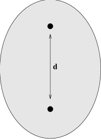
As the two endpoints can move independently, the two isospin components of the scattered brane waves can carry the causal time-delay information. Let us see how this looks like in the super Yang-Mills theory. The open string is now holographically projected to a shell of spherically symmetric Yang-Mills field configuration, as depicted in figure 10. The inner and outer radii are $R_{1}=g_{\rm eff}/U_{1}$ and $R_{2}=g_{\rm eff}/U_{2}$, respectively. Once the W-boson is hit by the incident brane wave on the first D3-brane, concentric spherical waves of the two isospin components will emanate. An observer sitting at spatial infinity on D3-branes will then perceive the radiation as originating from the same point in space (the center in figure 10), but with a time delay $\Delta\tau$. As is dictated by Eq.(2.7), the difference in ‘size’ coordinate of the wave-fronts in the super Yang-Mills theory equals exactly to $\Delta\tau$.

Figure 10: Yang-Mills theory view of the Thompson scattering

Having concluded that super Yang-Mills theory defined either in renormalizable or in DBI Lagrangians is not capable of encoding causality and locality of anti-de Sitter spacetime, we now ask what modifications, if possible, can do so. The answer to this question can be drawn again from Eq.(4.57). Expanding the infinite-order kernel for low-energy brane-wave, one finds

$$M_{\rm w}{\bf X}_{2}(t) = \sum_{n=-\infty}^{+\infty}(-)^{n}\int_{t\geq t^{\prime}}dt^{\prime}\,\bigg{\langle}t\bigg{|}{1\over\partial_{t}^{2}+(n/\Delta\tau)^{2}}\bigg{|}t^{\prime}\bigg{\rangle}\,Q{\bf E}^{(1)}(t^{\prime}).$$ (4.1)

$$= Q\sum_{n=-\infty}^{+\infty}\sum_{m=0}^{\infty}(-)^{m+n}\left({\Delta\tau\over n}\right)^{2m+2}{\cal O}_{2m}(t)$$

where

$${\cal O}_{2m}=\partial_{t}^{2m}{\bf E}(t).$$ (4.2)

Thus, the interaction of massive W-boson with the brane waves is governed by an infinite tower of higher-dimensional operators, ${\cal O}_{2m}$’s. Brane waves can be gauge or Higgs fields, so there will be similar higher-derivative operators including Higgs scalars. In $d=4,{\cal N}=4$ super Yang-Mills theory, operators of these structures are classified as long supermultiplets.

Perhaps, it should not be surpring that long supermultiplets are responsible for encoding causality and locality. After all, we have argued that string oscillator excitations are what is needed to for probing causality and locality. It has been already known [5, 6] that the long supermultiplets arise precisely from the massive string excitations, but the novelty of the above argument is that they can be seen explicitly even at the level of single W-boson.

Appendix: Effective Field Theory of String Endpoints

In this appendix, using covariant Green-Schwarz formalism, we will explain derivation of gauge-fixed, open string worldsheet action, Eqs.(2.2.1, 4.45). The derivation turns out somewhat nontrivial, as two Majorana-Weyl spinors of the covariant Green-Schwarz action are constrained both by $\kappa$-symmetry gauge-fixing and by open string boundary conditions. We will show that both requirements lead to so-called ‘D-brane gauge’ as a unique choice of the spinor projection. The ‘D-brane gauge’ has been proposed previously as a natural gauge-fixing condition of the $\kappa$ symmetry. Interestingly, we find that exactly the same condition also arises from the analysis of open string boundary conditions.

We will also derive, after integrating out string excitations, an effective field theory describing low-energy dynamics of two endpoints of the string. As pointed out in sections 2 and 4, the dynamics is described by a Lagrangian with infinite-order kernels, which turns out exactly the same as (two particle generalization of) the Pais-Uhlenbeck’s model. Remarkably, according to the analysis of Pais and Uhlenbeck, the particular infinite-order kernel is the one compatible with convergence, positive-definiteness and causality.

Appendix A Green-Schwarz Action in Flat Spacetime

Dynamics of an open F- or D-string stretched between the two parallel D3-branes, as depicted in Figure 2, is governed by the covariant Green-Schwarz action [37]. Denote bosonic and fermionic string coordinates as $(X^{M};\Theta^{A}_{\alpha})$ $(M=0,\cdots,9;A=1,2;\alpha=1,\cdots,32)$, which map worldsheet $\Sigma$ (spanned by $\sigma^{i}$ $(i=0,1)$) to coset superspace $Poincare(9,1|2)/SO(9,1)$. In Type IIB string theory, $\Theta^{1,2}$ are Majorana-Weyl spinors of same chirality. In the Nambu-Goto formulation, the worldsheet action is given by

$$I_{\rm string} = I_{\rm GS}+I_{\rm D3-Q}$$

$$I_{\rm GS} = -T\int_{\Sigma}d\tau d\sigma\,\Big{[}\sqrt{-{\rm det}L_{i}^{\hat{a}}L_{j}^{\hat{a}}}+i\int_{M_{3}}L^{\hat{a}}\wedge\overline{L}^{I}\tau_{3}^{IJ}\Gamma^{\hat{a}}\wedge L^{J}.$$ (A.1)

Here, $I_{\rm D3-Q}$ is a boundary action of the string endpoints, $M$ denotes a three-dimensional manifold whose boundary equals to the string worldsheet, and

$$L^{\hat{a}} = \delta_{M}^{\hat{a}}dX^{M}-i\overline{\Theta}^{A}\Gamma^{\hat{a}}d\Theta^{A},\qquad(\hat{a}=0,1,\cdots,9)$$

$$L^{I} = d\Theta^{I}.$$ (A.2)

are invariant Cartan one-forms of the coset superspace. The Wess-Zumino term in Eq.(A.1) is given by

$$L_{\rm WZ}=2idX^{\hat{a}}\!\wedge\!\left(\overline{\Theta}^{1}\Gamma^{\hat{a}}d\Theta^{1}-\overline{\Theta}^{2}\Gamma^{\hat{a}}d\Theta^{2}\right)-2\left(\overline{\Theta}^{1}\Gamma^{\hat{a}}d\Theta^{1}\right)\!\wedge\!\left(\overline{\Theta}^{2}\Gamma^{\hat{a}}d\Theta^{2}\right).$$ (A.3)

Apart from the boundary Lagrangian, the covariant Green-Schwarz action Eq.(A.1) is invariant under ${\cal N}=2$ global supersymmetry ($A=1,2$):

$$\delta_{\epsilon}\Theta^{A}=\epsilon^{A};\qquad\delta_{\epsilon}X^{\hat{a}}=i\overline{\epsilon}^{A}\Gamma^{\hat{a}}\Theta^{A},$$ (A.4)

and local $\kappa$ symmetry, when expressed in terms of worldsheet scalar spinors $\tilde{\kappa}$ ,

$$\delta_{\tilde{\kappa}}\,\Theta^{A}=\left(1+(-)^{A}{\cal P}\right)\tilde{\kappa}^{A},\qquad\delta_{\kappa}\,X^{\hat{a}}=i\overline{\Theta}^{A}\Gamma^{\hat{a}}\delta_{\tilde{\kappa}}\Theta^{A},$$ (A.5)

where

$${\cal P}={1\over 2}{L^{\hat{a}}\wedge L^{\hat{b}}\over\sqrt{-h}}\Gamma^{\hat{a}\hat{b}},\qquad{\cal P}^{2}=1.$$ (A.6)

A.1 Open String Boundary Conditions

The last term in Eq.(A.1) is the Lagrangian describing interaction of the open string endpoints with gauge and Higgs fields on the worldvolume of the two D3-branes. Denoting the $d=4,{\cal N}=4$ vector supermultiplet as $(A,\lambda)$, the boundary Lagrangian in the lowest order in derivative expansion reads

$$L_{\rm D3-Q}=Q\oint_{\partial\Sigma}d\tau\dot{X}^{\hat{a}}\left(A_{\hat{a}}(X)-\overline{\lambda}(X)\Gamma_{\hat{a}}\theta\right).$$ (A.7)

The boundary action represents turning on gauge and Higgs fields on the D3-brane worldvolume. The boundary conditions, derived from variation of the Green-Schwarz action, are given by

$$D\quad : \qquad\delta X^{\perp}=0,\qquad\overline{\Theta}^{1}\Gamma^{\perp}\delta\Theta^{1}+\overline{\Theta}^{2}\Gamma^{\perp}\delta\Theta^{2}=0$$ (A.8)

$$N\quad : \qquad\Pi^{|\hskip-0.85355pt|}_{\sigma}=0,\qquad\overline{\Theta}^{1}\Gamma^{|\hskip-0.85355pt|}\delta\Theta^{1}-\overline{\Theta}^{2}\Gamma^{|\hskip-0.85355pt|}\delta\Theta^{2}=0,$$ (A.9)

for Dirichlet and Neumann directions, respectively. To proceed further with gauge fixing, one will need to find linear boundary conditions for fermions that are consistent with Eqs.(A.8, A.9). Because of sign difference between $A=1,2$ terms in Eqs.(A.8, A.9), a unique choice of the linear boundary condition is of the form

$$\Theta^{A}=\Gamma_{5}{{\cal M}^{A}}_{B}\Theta^{B},\qquad\Gamma_{5}\equiv\Gamma^{0}\Gamma^{1}\cdots\Gamma^{3},$$ (A.10)

where $(2\times 2)$ matrix ${\cal M}$ is determined to be ${\cal M}_{AB}=\epsilon_{AB}$ by the requirement that the boundary condition is compatible with Majorana and Weyl conditions and with invertibility of Eq.(A.10). Hence, for open Green-Schwarz superstring attached between the two D3-branes, the boundary conditions are:

$$\delta X^{\perp}=0, \partial_{\sigma}X^{|\hskip-0.85355pt|}=0$$

$$\left(\delta_{AB}-\Gamma_{5}\epsilon_{AB}\right)\Theta^{B}=0 \left(\delta_{AB}+\Gamma_{5}\epsilon_{AB}\right)\partial_{\sigma}\Theta^{B}=0.$$ (A.11)

A.2 Gauge Fixing

Due to the local $\kappa$-symmetry, half of the degrees of freedom of $\Theta^{1,2}$’s are redundant. Since the spinors $\Theta^{1,2}$ have the same chirality, the $\kappa$-symmetry may be gauge fixed conveniently by setting $\Theta^{1}=\Gamma_{5}\Theta^{2}\equiv{1\over 2}\Psi$. Using equation of motion for $L^{\hat{a}}$’s, a straightforward calculation yields the $\kappa$-gauge-fixed action

$$I_{\rm GS}=T\int\!\!\!\int d\tau d\sigma\,\left[\sqrt{-{\rm det}\partial_{i}X^{\hat{a}}\partial_{j}X^{\hat{a}}}+{i\over 2}dX^{\hat{a}}\wedge(\overline{\Psi}\Gamma^{\hat{a}}d\Psi)\,\right].$$ (A.12)

In the gauge-fixed action, half of ${\cal N}=2$ supersymmetry is realized linearly

$$\delta_{\epsilon}X^{\hat{a}}=i\overline{\epsilon}\Gamma^{\hat{a}}\Psi,\qquad\delta_{\epsilon}\Psi=-{1\over 2}{dX^{\hat{a}}\wedge dX^{\hat{b}}\over|\!\!|dX\wedge dX|\!\!|}\Gamma^{\hat{a}\hat{b}}\epsilon,$$ (A.13)

and the other half as a nonlinear fermionic symmetry

$$\delta_{\xi}X^{\hat{a}}=0,\qquad\delta_{\xi}\Psi=\xi.$$ (A.14)

For the reparametrization invariance, we will choose the static gauge $\sigma^{0}=t$, $\sigma^{1}=r$. After expanding the action to quadratic order and reinstating the speed of light $c$, one obtains the gauge-fixed action of the open string as:

$$I_{\rm GS}=I_{\rm string}+I_{\rm D3-Q}$$ (A.15)

where

$$I_{\rm string} = \int\!dt\,\left[-M_{\rm w}+{T\over 2}\int_{r_{1}}^{r_{2}}dr\,\left({1\over c^{2}}(\partial_{t}{\bf X})^{2}-(\partial_{r}{\bf X})^{2}\right)+\cdots\right]$$ (A.16)

$$I_{\rm D3-Q} = \!\!\!\!\sum_{I=1,2}\int dt\,Q_{\rm I}\left[A_{0}^{\rm(I)}({\bf r},t)+{1\over c}\dot{\bf X}_{\rm I}(t)\cdot{\bf A}^{\rm(I)}({\bf r},t)\right]_{{\bf r}={\bf X}_{\rm I}(t)},\qquad(Q_{1}=-Q_{2}=\pm 1).$$

A.3 Low-Energy Effective Lagrangian of String Endpoints

We will begin with solving the equations of motion for ${\bf X}(t,r)$, subject to fixed but arbitrary location of the string endpoints, ${\bf X}_{1,2}(t)$. Consider a Fourier transformed, harmonic solution

$$\tilde{\bf X}(\omega,r) = \int dte^{+i\omega t}{\bf X}(t,r)$$

$$= {\bf a}(\omega)e^{-i\omega(t-r/c)}+\tilde{\bf a}(\omega)e^{-i\omega(t+r/c)}.$$

The boundary condition specified,

$$\tilde{\bf X}(\omega,r)\bigg{|}_{r=r_{1}}=\tilde{\bf X}_{1}(\omega),\qquad\tilde{\bf X}(\omega,r)\bigg{|}_{r=r_{2}}=\tilde{\bf X}_{2}(\omega),$$

relates the spectral amplitudes ${\bf a}(\omega),\tilde{\bf a}(\omega)$ uniquely to the (Fourier transformed) string endpoints $\tilde{\bf X}_{1,2}(\omega)$. Using the relation, it is possible to express normal derivatives at the string endpoints

$$\partial_{r}\tilde{\bf X}_{1}(\omega)\equiv\partial_{r}\tilde{\bf X}(\omega,r)\bigg{|}_{r=r_{1}},\qquad\tilde{\bf X}_{2}(\omega)\equiv\partial_{r}\tilde{\bf X}(\omega,r)\bigg{|}_{r=r_{2}}$$

in terms of $\tilde{\bf X}_{1,2}(\omega)$. The result is ($\Delta t\equiv\Delta r/c$)

$$\partial_{r}\tilde{\bf X}_{1}(\omega)=-{\omega\Delta t\over\sin\omega\Delta t}\left({\tilde{\bf X}_{1}(\omega)\cos\omega\Delta t-\tilde{\bf X}_{2}(\omega)\over c\Delta t}\right)$$

$$\partial_{r}\tilde{\bf X}_{2}(\omega)=-{\omega\Delta t\over\sin\omega\Delta t}\left({\tilde{\bf X}_{1}(\omega)-\tilde{\bf X}_{2}(\omega)\cos\omega\Delta t\over c\Delta t}\right).$$ (A.18)

In order to obtain an effective action for the string endpoints, we will need to integrate out massive string excitations. As the string action, $I_{\rm string}$, is quadratic in ${\bf X}(r,t)$ at leading order, it amounts to imposing the equation of motion of ${\bf X}(r,t)$ back to the action, Eq.(A.16). One then obtains, after Fourier-transform back to ${\bf X}_{1,2}(t)$,

$$I_{\rm string}=\int\!dt\,\,\left[-M_{\rm w}-{T\over 2}\Big{(}{\bf X}_{2}(t)\cdot\partial_{r}{\bf X}_{2}(t)-{\bf X}_{1}(t)\cdot\partial_{r}{\bf X}_{1}(t)\Big{)}+\cdots\right].$$ (A.19)

The string action is now expressed entirely in terms of boundary data of the open string positions on the two D3-branes.

Inserting Eq.(A.18) to Eq.(A.19), one finally obtains the low-energy effective action of the string endpoints:

$$I_{\rm GS} = I_{\rm string}+I_{\rm D3-Q}$$ (A.20)

$$I_{\rm string} = \int dt\,\left[-M_{\rm w}-{T\over 2}\sum_{I,J=1,2}{\bf X}_{I}(t){\cal K}^{\rm flat}_{IJ}\left(\Delta t\partial_{t}\right){\bf X}_{J}(t)\,\,\right]$$

$$I_{\rm D3-Q} = \sum_{\rm I=1,2}\int dt\,Q_{\rm I}\left[A_{0}^{\rm(I)}({\bf r},t)+{1\over c}\dot{\bf X}_{\rm I}(t)\cdot{\bf A}^{\rm(I)}({\bf r},t)\right]_{{\bf r}={\bf X}_{\rm I}(t)},\qquad(Q_{1}=-Q_{2}=\pm 1).$$

In the action, $I_{\rm string}$, the infinite-order kernels are defined by:

$${\cal K}^{\rm flat}_{11}={\cal K}^{\rm flat}_{22} = +{1\over\Delta r}\left({\Delta t\partial_{t}\over\tanh\Delta t\partial_{t}}\right)$$

$${\cal K}^{\rm flat}_{12}={\cal K}^{\rm flat}_{21} = -{1\over\Delta r}\left({\Delta t\partial_{t}\over\sinh\Delta t\partial_{t}}\right).$$ (A.21)

Let us now focus on the Thomson scattering by D3-brane waves, studied in section 2. Initially, the radiation field is present only for the first D3-brane, viz. $A_{0}^{(2)}={\bf A}^{(2)}=0$. In this case, the equation of motion for ${\bf X}_{2}(t)$ is reduced simply to

$$\left(\cosh\Delta t\partial_{t}\right)\,{\bf X}_{2}(t)={\bf X}_{1}(t),$$ (A.22)

viz. a retardation relation

$${\bf X}_{2}(t)=\int dt^{\prime}\bigg{\langle}t\bigg{|}{1\over\cosh\Delta t\partial_{t}}\bigg{|}t^{\prime}\bigg{\rangle}\,{\bf X}_{1}(t^{\prime}).$$ (A.23)

After ${\bf X}_{2}(t)$ is integrated out of $I_{\rm string}$ using Eq.(A.22), the low-energy effective Lagrangian for the Thomson scattering process is obtained:

$$L_{\rm Thomson}= - M_{\rm w}+{M_{\rm w}\over 2}\dot{\bf X}_{1}(t)\left({\tanh\Delta t\partial_{t}\over\Delta t\partial_{t}}\right)\dot{\bf X}_{1}(t)+\cdots$$ (A.24)

$$+ Q\left[A_{0}^{(1)}({\bf r},t)+{1\over c}\dot{\bf X}_{1}\cdot{\bf A}^{(1)}({\bf r},t)\right]_{{\bf r}={\bf X}_{1}(t)}.$$

The Eqs.(2.12, 2.13) follow immediately from the above effective Lagrangian and the retardation relation Eq.(A.22).

Appendix B Green-Schwarz Action in Anti-de Sitter Spacetime

The Green-Schwarz action in $AdS_{5}\times S^{5}$ can be obtained in a closed form via super-coset space construction [38] . In Nambu-Goto form, the action reads

$$I_{\rm AdS}=T\int\!\!\!\int d\tau d\sigma\,\left[\sqrt{-{\rm det}L_{i}^{\hat{a}}L_{j}^{\hat{a}}}+4i\int_{0}^{1}dsL_{i}^{\hat{a}}(s)\overline{\Theta}\tau_{3}\Gamma^{\hat{a}}L_{j}(s)\,\right].$$ (B.25)

Here, ${\hat{a}}=(a,a^{\prime})=(0,1,\cdots,4,5,\cdots,9)$, $I,J=1,2$ and $\tau_{1,2,3}$ are Pauli matrices. The invariant worldsheet one-forms $L^{I}(s)$ and $L^{\hat{a}}(s)$ are given by

$$L^{I}(s) = \left({\sinh s{\cal M}\over{\cal M}}{\cal D}\Theta\right)^{I}$$

$$L^{\hat{a}}(x) = e^{\hat{a}}_{M}dX^{M}-4i\overline{\Theta}^{I}\Gamma^{\hat{a}}\left({\sinh^{2}{1\over 2}s{\cal M}\over{\cal M}^{2}}{\cal D}\Theta\right)^{I},$$ (B.26)

where $(X^{M},\Theta^{I})$ are the bosonic and fermionic F-string coordinates and

$$\left({\cal M}^{2}\right)^{IJ} = \left[\gamma^{a^{\prime}}(i\tau_{2}\Theta)^{I}\overline{\Theta}^{J}\gamma^{a^{\prime}}-\gamma^{a}(i\tau_{2}\Theta)^{I}\overline{\Theta}^{J}\gamma^{a}\right]+{1\over 2}\left[\gamma^{a^{\prime}b^{\prime}}\Theta^{I}(\overline{\Theta}i\tau_{2})^{J}\gamma^{a^{\prime}b^{\prime}}-\gamma^{ab}\Theta^{I}(\overline{\Theta}i\tau_{2})^{J}\gamma^{ab}\right]$$

$$({\cal D}\Theta)^{I} = \left(\partial+{1\over 4}\omega^{\hat{a}\hat{b}}\Gamma_{\hat{a}\hat{b}}\right)\Theta^{I}+{1\over 2}E^{\hat{a}}\Gamma_{\hat{a}}\left(\tau_{2}\Theta\right)^{I}.$$ (B.27)

Also, $L^{I}\equiv L^{I}(s=1)$, $L^{\hat{a}}\equiv L^{\hat{a}}(s=1)$.

The action is invariant under the ${\cal N}=2$ global supersymmtry and local $\kappa$-symmetry. Expressing again in terms of worldsheet scalar spinors, the symmetry transformations rules are essentially the same as Eqs.(A.5, 6), except now the indices are repeated over $AdS_{5}$ and $S^{5}$. :

B.1 Gauge Fixing

In order to fix the local $\kappa$-symmetry, it turns out most convenient to make a change of variable $R=g_{\rm eff}/U$ and use the Poincaré coordinates. Up to the conformal rescaling, the ten-dimensional spacetime is flat. To proceed in an analogous manner to the flat spacetime situation, we will follow the observation of Kallosh [40, 41, 42] and take the gauge-fixing

$$\Theta^{I}_{-}=0\qquad{\rm where}\qquad\Theta^{I}_{\pm}\equiv({\cal P}_{\pm}\Theta)^{I},\quad{\cal P}_{\pm}^{IJ}={1\over 2}\left(\tau_{0}\pm i\Gamma_{5}\tau_{2}\right)^{IJ}.$$ (B.28)

The $\kappa$-gauge-fixed action is quartic in fermions. However, if one makes a change of variable to the ‘size’ variable, $R=g_{\rm eff}/U$, as mentioned in seciton 4, the quartic fermon terms are turned into quadratic ones only. Moreover, in the $R$-coordinates, as we will see below, the reparametrization gauge-fixed action also simplifies considerably .

Again, choosing the static gauge $\sigma^{0}=t$, $\sigma^{1}=R$, one finds that the gauge-fixed Green-Schwarz action of the open string in anti-de Sitter spacetime is given by:

$$I_{\rm AdS}=\left(L_{\rm string}+L_{\rm D3-Q}\right)$$ (B.29)

where

$$I_{\rm string} = \int dt\,\left[-M_{\rm w}+{g_{\rm eff}\over 2}\int_{R_{1}}^{R_{2}}{dR\over R^{2}}\left({1\over c^{2}}(\partial_{t}{\bf X})^{2}-(\partial_{R}{\bf X})^{2}\right)+\cdots\right]$$ (B.30)

$$L_{\rm D3-Q} = \!\!\!\sum_{I=1,2}\!\int dt\,Q_{\rm I}\left[A_{0}^{\rm(I)}({\bf r},t)+{1\over c}\dot{\bf X}_{\rm I}(t)\cdot{\bf A}^{\rm(I)}({\bf r},t)\right]_{{\bf r}={\bf X}_{\rm I}(t)},\quad(Q_{1}=-Q_{2}=\pm 1).$$ (B.31)

and the boundary interaction action is exactly the same in the flat spacetime.

B.2 Low-Energy Effective Lagrangian of String Endpoints

One can obtain low-energy effective Lagrangian of the string endpoints repeating steps of flat spacetime case, section A.2. After Fourier transformation, a harmonic solution of the string coordinate $\tilde{\bf X}(\omega,R)$ now takes a form

$$\tilde{\bf X}(\omega,R) = \int dte^{+i\omega t}{\bf X}(t,R)$$

$$= {\bf a}(\omega)\left(1-i\omega{R\over c}\right)e^{-i\omega(t-R/c)}+\tilde{\bf a}(\omega)\left(1+i\omega{R\over c}\right)e^{-i\omega(t+R/c)},$$

where the harmonic modes are expanded in terms of the Hankel functions, $H^{(\pm)}_{3/2}(\omega R)$. Eliminating ${\bf a}(\omega),\tilde{\bf a}(\omega)$ between $\tilde{\bf X}_{1,2}(\omega)$ and $\partial_{z}\tilde{\bf X}_{1,2}(\omega)$, one finds relations $(\Delta\tau\equiv\Delta z/c)$

$${1\over R_{1}}\partial_{R}\tilde{\bf X}_{1}(\omega) = {\omega^{2}\over{\cal N}}\left[\left(\sin\omega\Delta\tau+\omega{R_{2}\over c}\cos\omega\Delta\tau\right)\tilde{\bf X}_{1}(\omega)-\omega{R_{1}\over c}\tilde{\bf X}_{2}(\omega)\right]$$

$${1\over R_{2}}\partial_{R}\tilde{\bf X}_{2}(\omega) = {\omega^{2}\over{\cal N}}\left[\omega{R_{2}\over c}\tilde{\bf X}_{1}(\omega)+\left(\sin\omega\Delta\tau-\omega{R_{1}\over c}\cos\omega\Delta\tau\right)\tilde{\bf X}_{2}(\omega)\right],$$ (B.32)

where

$${\cal N}=\left(1+\omega^{2}{R_{1}R_{2}\over c^{2}}\right)\sin\omega\Delta\tau-\omega\Delta\tau\cos\omega\Delta\tau.$$

Imposing the equation of motion for ${\bf X}(t,z)$ to the action Eq.(B.30), one obtains

$$I_{\rm string}=\int dt\,\left[-M_{\rm w}-{g_{\rm eff}\over 2}\left({1\over R_{2}^{2}}{\bf X}_{2}(t)\cdot\partial_{R}{\bf X}_{2}(t)-{1\over R_{1}^{2}}{\bf X}_{1}(t)\cdot\partial_{R}{\bf X}_{1}(t)\right)+\cdots\right].$$ (B.33)

Inserting Eq.(B.32) to the action Eq.(B.33), after Fourier-transforming back, one finally arrives at the low-energy effective action of the string endpoints in anti-de Sitter spacetime:

$$I_{\rm AdS} = \left(I_{\rm string}+I_{\rm D3-Q}\right)$$ (B.34)

$$I_{\rm string} = \int dt\,\left[-M_{\rm w}-{g_{\rm eff}\over 2}\sum_{I,J=1,2}{\bf X}_{I}(t)\cdot{\cal K}_{IJ}^{\rm AdS}(\Delta\tau\partial_{t})\cdot{\bf X}_{J}(t)+\cdots\right]$$

$$I_{\rm D3-Q} = \sum_{I=1,2}\int dt\,Q_{\rm I}\left[A_{0}^{\rm(I)}({\bf r},t)+{1\over c}\dot{\bf X}_{\rm I}(t)\cdot{\bf A}^{\rm(I)}({\bf r},t)\right]_{{\bf r}={\bf X}_{\rm I}(t)},\qquad(Q_{1}=-Q_{2}=\pm 1).$$

The infinite-order kernels in the action $I_{\rm string}$ are now given by:

$${\cal K}_{11}^{\rm AdS} = -{1\over R_{1}}\left(1+{R_{2}/c\over\Delta\tau}{\Delta\tau\partial_{t}\over\tanh\Delta\tau\partial_{t}}\right)\left(1-{R_{1}R_{2}\over c^{2}}\partial_{t}^{2}-{\Delta\tau\partial_{t}\over\tanh\Delta\tau\partial_{t}}\right)^{-1}$$

$${\cal K}_{22}^{\rm AdS} = +{1\over R_{2}}\left(1-{R_{1}/c\over\Delta\tau}{\Delta\tau\partial_{t}\over\tanh\Delta\tau\partial_{t}}\right)\left(1-{R_{1}R_{2}\over c^{2}}\partial_{t}^{2}-{\Delta\tau\partial_{t}\over\tanh\Delta\tau\partial_{t}}\right)^{-1}$$

$${\cal K}_{12}^{\rm AdS} = {\cal K}_{21}^{\rm AdS}=+{1\over\Delta R}\left({\Delta\tau\partial_{t}\over\sinh\Delta\tau\partial_{t}}\right)\left(1-{R_{1}R_{2}\over c^{2}}\partial_{t}^{2}-{\Delta\tau\partial_{t}\over\tanh\Delta\tau\partial_{t}}\right)^{-1}.$$ (B.35)

Let us again consider Thomson scattering of D3-brane wave, studied in section 4, by setting $A_{0}^{(2)}={\bf A}^{(2)}=0$. From Eq.(B.34), equation of motion for ${\bf X}_{2}(t)$ yields a retardation relation

$$\left(1+{R_{1}\over R_{2}}\left({\Delta\tau\partial_{t}\over\tanh\Delta\tau\partial_{t}}-1\right)\right)\left({\sinh\Delta\tau\partial_{t}\over\Delta\tau\partial_{t}}\right)\,{\bf X}_{2}(t)={\bf X}_{1}(t).$$ (B.36)

Integrating out ${\bf X}_{2}(t)$ from the action $I_{\rm string}$, using Eq.(B.36), one finally obtains the low-energy effective Lagrangian for the Thomson scattering of D3-brane waves:

$$L_{\rm Thomson}= - M_{\rm w}+{M_{\rm w}\over 2}\dot{\bf X}_{1}(t)\left(1+{R_{1}\over R_{2}}\left({\Delta\tau\partial_{t}\over\tanh\Delta\tau\partial_{t}}-1\right)\right)^{-1}\dot{\bf X}_{1}(t)+\cdots$$ (B.37)

$$+ Q\left[A^{(1)}_{0}({\bf r},t)+{1\over c}\dot{\bf X}_{1}(t)\cdot{\bf A}^{(1)}({\bf r},t)\right]_{{\bf r}={\bf X}_{1}(t)}.$$

From the effective Lagrangian Eq.(B.37) and the retardation relation Eq.(B.36), one gets easily the equations of motion of string endpoints, Eqs.(4.44, 4.45).

References

- [1] J. Maldacena, Adv. Theo. Math. Phys. 2 (1998) 231.
- [2] G. ‘t Hooft, Dimensional Reduction in Quantum Gravity, in ‘Salamfest’, eds. A. Ali and J. Ellis, pp. 284 - 296 (World Scientific Co. Singapore, 1993).
- [3] L. Susskind, J. Math. Phys. 36 (1995) 6377.
- [4] C.B. Thorn, Reformulating String Theory With The Expansion, in ‘Sakharov Conference’, eds. L.V. Keldysh and V.Ya. Fainberg, pp. 447 - 454 (Nova Science, 1992).
- [5] S.S. Gubser, I.R. Klebanov and A.M. Polyakov, Phys. Lett. 428B (1998) 105.
- [6] E. Witten, Adv. Theo. Math. Phys. 2 (1998) 253.
- [7] L. Susskind and E. Witten, The Holographic Bound in Anti-de Sitter Space, hep-th/9805114.
- [8] V. Balasubramanian, P. Kraus and A. Lawrence, Phys. Rev. D59 (1999) 46003; V. Balasubramanian, S. Giddings and A. Lawrence, What Do CFTs Can Tell Us About Anti-de Sitter Space-Times?, hep-th/9902052.
- [9] T. Banks, M.R. Douglas, G.T. Horowitz and E. Martinec, AdS Dynamics from Conformal Field Theory, hep-th/9808016.
- [10] J. Polchinski and A. Peet, UV/IR Relations in AdS Dynamics, hep-th/9809022.
- [11] G.T. Horowitz and N. Itzhaki, Black Holes, Shock Waves, and Causality in the AdS/CFT Correspondence, hep-th/9901012.
- [12] J. Polchinski, S-Matrices from AdS Spacetime, hep-th/9901076.
- [13] L. Susskind, Holography in the Flat Space Limit, hep-th/9901079.
- [14] D. Kabat and G. Lifschytz, Gauge Theory Origins of Supergravity Causal Structure, hep-th/9902073.
- [15] G. ‘t Hooft, Comm. Math. Phys. 86 (1982) 449; ibid 88 (1983) 1.
- [16] See, for example, J.D. Jackson, Classical Electrodynamics, 3rd Edition, (Addison-Wesley, Reading, 1998).
- [17] S.J. Gates, M.T. Grisaru, M. Rocek and W. Siegel, “Superspace” (Benjamin Cummings, 1987).
- [18] M. Dine and N. Seiberg, Phys. Lett. 409B (1997) 239.
- [19] J. Maldacena, Phys. Rev. D57 (1998) 3736.
- [20] V. Periwal and R. von Unge, Accelerating D-branes, hep-th/9801121.
- [21] M. Berkooz, A Proposal of Some Microscopic Aspects of AdS/CFT Correspondence, hep-th/9807230.
- [22] D. Lowe and R. von Unge, J. High Energy Phys. 9811 (1998) 14.
- [23] M.R. Douglas and W. Taylor IV, Branes in the Bulk of Anti-de Sitter Space, hep-th/9807225.
- [24] S.R. Das, Brane Waves, Yang-Mills Theories and Causality, hep-th/9901004.
- [25] T. Yoneya, Mod. Phys. Lett. A4 (1989) 1587.
- [26] E. Witten, Nucl. Phys. B460 (1996) 335.
- [27] H. Yukawa, Phys. Rev. 77 (1950) 219; ibid 80 (1950) 1047.
- [28] A. Pais and G.E. Uhlenbeck, Phys. Rev. 79 (1950) 145.
- [29] S.-J. Rey and J.-T. Yee, Nucl. Phys. B526 (1998) 229.
- [30] S.-J. Rey and J.-T. Yee, Macroscopic Strings as Heavy Quarks in Large-N Gauge Theories and Anti-de Sitter Supergravity, hep-th/9803001.
- [31] J. Maldacena, Phys. Rev. Lett. 80 (1998) 4859.
- [32] D. Bak and C. Lee, Nucl. Phys. B403 315 (1993); ibid 424 (1994) 124.
- [33] D. Bak and H. Min, Phys. Rev. D56 6665 (1997).
- [34] S.-J. Rey, S. Theisen and J.-T. Yee, Nucl. Phys. B527 (1998) 171.
- [35] A. Brandhuber, N. Itzhaki, J. Sonnenschein and S. Yankielowicz, Phys. Lett. 434B (1998) 36.
- [36] S.H. Shenker, Another Length Scale in String Theory?, hep-th/9509132.
- [37] M.B. Green and J.H. Schwarz, Phys. Lett. 136B (1984) 367.
- [38] R.R. Metsaev and A.A. Tseytlin, Nucl. Phys. B533 (1998) 109.
- [39] J. Park and S.-J. Rey, J. High Energy Phys. 9811 (1998) ppp.
- [40] R. Kallosh, Superconformal Actions in Killing Gauge, hep-th/9807206.
- [41] R. Kallosh and J. Rahmfeld, Phys. Lett. 443B (1998) 143.
- [42] R. Kallosh and A.A. Tseytlin, J. High Energy Phys. 9810 (1998) 16.
- [43] A. Rajaraman and M. Rozali, On the Quantization of GS String on , hep-th/9902046.