Classical and quantum gravitational instabilities, can, respectively, inflate and warm up a primordial Universe satisfying a superstring-motivated principle of “Asymptotic Past Triviality”. A physically viable big bang is thus generated without invoking either large fine-tunings or a long period of post-big bang inflation. Properties of the pre-bangian Universe can be probed through its observable relics, which include: i) a (possibly observable) stochastic gravitational-wave background; ii) a (possible) new mechanism for seeding the galactic magnetic fields; iii) a (possible) new source of large-scale structure and CMB anisotropy.

1 INTRODUCTION

I would like to begin this talk by asking a very simple question: Did the Universe start “small”? The naive answer is: Yes, of course! However, a serious answer can only be given after defining the two keywords in the question: What do we mean by “start”? and What is “small” relative to? In order to be on the safe side, let us take the “initial” time to be a bit larger than Planck’s time, $t_{P}\sim 10^{-43}\;\rm{s}$. Then, in standard Friedmann–Robertson–Walker (FRW) cosmology, the initial size of the (presently observable) Universe was about $10^{-2}~{}\rm{cm}$. This is of course tiny w.r.t. its present size ($\sim 10^{28}~{}\rm{cm}$), yet huge w.r.t. the horizon at that time, i.e. w.r.t. $l_{P}=ct_{P}\sim 10^{-33}~{}\rm{cm}$. In other words, a few Planck times after the big bang, our observable Universe consisted of $(10^{30})^{3}=10^{90}$ Planckian-size, causally disconnected regions.

More precisely, soon after $t=t_{P}$, the Universe was characterized by a huge hierarchy between its Hubble radius and inverse temperature on one side, and its spatial-curvature radius and homogeneity scale on the other. The relative factor of (at least) $10^{30}$ appears as an incredible amount of fine-tuning on the initial state of the Universe, corresponding to a huge asymmetry between time and space derivatives. Was this asymmetry really there? And if so, can it be explained in any more natural way?

It is well known that a generic way to wash out inhomogeneities and spatial curvature consists in introducing, in the history of the Universe, a long period of accelerated expansion, called inflation [1]. This still leaves two alternative solutions: either the Universe was generic at the big bang and became flat and smooth because of a long post-bangian inflationary phase; or it was already flat and smooth at the big bang as the result of a long pre-bangian inflationary phase.

Assuming, dogmatically, that the Universe (and time itself) started at the big bang, leaves only the first alternative. However, that solution has its own problems, in particular those of fine-tuned initial conditions and inflaton potentials. Besides, it is quite difficult to base standard inflation in the only known candidate theory of quantum gravity, superstring theory. Rather, as we shall argue, superstring theory gives strong hints in favour of the second (pre-big bang) possibility through two of its very basic properties, the first in relation to its short-distance behaviour, the second from its modifications of General Relativity even at large distance. Let us briefly comment on both.

2 (Super)String inspiration

2.1 Short Distance

Since the classical (Nambu–Goto) action of a string is proportional to the area $A$ of the surface it sweeps, its quantization must introduce a quantum of length $\lambda_{s}$ through:

$$S/\hbar=A/\lambda_{s}^{2}\;.$$ (1)

This fundamental length, replacing Planck’s constant in quantum string theory [2], plays the role of a minimal observable length, of an ultraviolet cut-off. Thus, in string theory, physical quantities are expected to be bound by appropriate powers of $\lambda_{s}$, e.g.

$$H^{2}\sim R\sim G\rho<\lambda_{s}^{-2}$$

$$k_{B}T/\hbar<c\lambda_{s}^{-1}$$

$$R_{comp}>\lambda_{s}\;.$$ (2)

In other words, in quantum string theory (QST), relativistic quantum mechanics should solve the singularity problems in much the same way as non-relativistic quantum mechanics solved the singularity problem of the hydrogen atom by putting the electron and the proton a finite distance apart. By the same token, QST gives us a rationale for asking daring questions such as: What was there before the big bang? Certainly, in no other present theory, can such a question be meaningfully asked.

2.2 Large Distance

Even at large distance (low-energy, small curvatures), superstring theory does not automatically give Einstein’s General Relativity. Rather, it leads to a scalar-tensor theory of the JBD variety. The new scalar particle/field $\phi$, the so-called dilaton, is unavoidable in string theory, and gets reinterpreted as the radius of a new dimension of space in so-called M-theory [3]. By supersymmetry, the dilaton is massless to all orders in perturbation theory, i.e. as long as supersymmetry remains unbroken. This raises the question: Is the dilaton a problem or an opportunity? My answer is that it is possibly both; and while we can try to avoid its potential dangers, we may try to use some of its properties to our advantage …  Let me discuss how.

In string theory $\phi$ controls the strength of all forces, gravitational and gauge alike. One finds, typically:

$$l_{P}^{2}/\lambda_{s}^{2}\sim\alpha_{gauge}\sim e^{\phi}\;,$$ (3)

showing the basic unification of all forces in string theory and the fact that, in our conventions, the weak-coupling region coincides with $\phi\ll-1$. In order not to contradict precision tests of the Equivalence Principle and of the constancy of the gauge and gravitational couplings in the recent past (possibly meaning several million years!) we require [4] the dilaton to have a mass and to be frozen at the bottom of its own potential today. This does not exclude, however, the possibility of the dilaton having evolved cosmologically (after all the metric did!) within the weak coupling region where it was practically massless. The amazing (yet simple) observation [5] is that, by so doing, the dilaton may have inflated the Universe!

A simplified argument, which, although not completely accurate, captures the essential physical point, consists in writing the ($k=0$) Friedmann equation:

$$3H^{2}=8\pi G\rho\;,$$ (4)

and in noticing that a growing dilaton (meaning through (3) a growing $G$) can drive the growth of $H$ even if the energy density of standard matter decreases in an expanding Universe. This new kind of inflation (characterized by growing $H$ and $\phi$) has been termed dilaton-driven inflation (DDI). The basic idea of pre-big bang cosmology [5, 6, 7] is thus illustrated in Fig. 1: the dilaton started at very large negative values (where it is massless), ran over a potential hill, and finally reached, sometime in our recent past, its final destination at the bottom of its potential ($\phi=\phi_{0}$). Incidentally, as shown in Fig. 1, the dilaton of string theory can easily roll-up —rather than down— potential hills, as a consequence of its non-standard coupling to gravity.

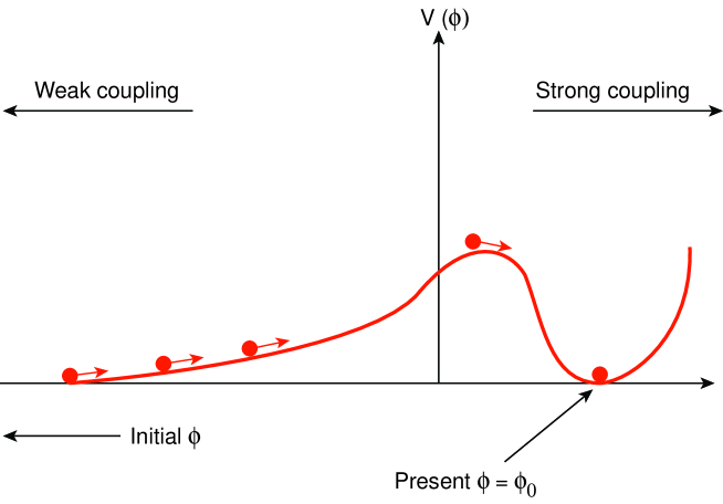
Figure 1:

DDI is not just possible. It exists as a class of (lowest-order) cosmological solutions thanks to the duality symmetries of string cosmology. Under a prototype example of these symmetries, the so-called scale-factor duality [5], a FRW cosmology evolving (at lowest order in derivatives) from a singularity in the past is mapped into a DDI cosmology going towards a singularity in the future. Of course, the lowest order approximation breaks down before either singularity is reached. A (stringy) moment away from their respective singularities, these two branches can easily be joined smoothly to give a single non-singular cosmology, at least mathematically. Leaving aside this issue for the moment (see Section V for more discussion), let us go back to DDI. Since such a phase is characterized by growing coupling and curvature, it must itself have originated from a regime in which both quantities were very small. We take this as the main lesson/hint to be learned from low-energy string theory by raising it to the level of a new cosmological principle [8] of “Asymptotic Past Triviality”.

3 Asymptotic Past Triviality

The concept of Asymptotic Past Triviality (APT) is quite similar to that of “Asymptotic Flatness”, familiar from General Relativity [9]. The main differences consist in making only assumptions concerning the asymptotic past (rather than future or space-like infinity) and in the additional presence of the dilaton. It seems physically (and philosophically) satisfactory to identify the beginning with simplicity (see e.g. entropy-related arguments concerning the arrow of time). What could be simpler than a trivial, empty and flat Universe? Nothing of course! The problem is that such a Universe, besides being uninteresting, is also non-generic. By contrast, asymptotically flat/trivial Universes are initially simple, yet generic in a precise mathematical sense. Their definition involves exactly the right number of arbitrary “integration constants” (here full functions of three variables) to describe a general solution (one with some general, qualitative features, though). This is why, by its very construction, this cosmology cannot be easily dismissed as being fine-tuned.

It is useful to represent the situation in a Carter–Penrose diagram, as in Fig. 2. Here past infinity consists of two pieces: time-like past infinity, which is shrunk to a point $I_{-}$, and past null-infinity, $\cal{I}_{-}$ represented by a line at $45$ degrees. Note that this region of the diagram is “non-physical” in FRW cosmology, since it lies behind (i.e. before) the big bang singularity (also shown in the diagram). Instead, we shall be giving initial data infinitesimally close to $I_{-}$ and $\cal{I}_{-}$, and ask whether they will evolve in such a way as to generate a physically interesting big bang-like state at some later time. Generating so much from so little looks a bit like a miracle. However, we will argue that it is precisely what should be expected, owing to well-known classical and quantum gravitational instabilities.

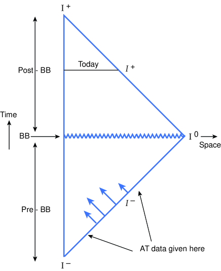
Figure 2:

4 Inflation as a classical gravitational instability

The assumption of APT entitles us to treat the early history of the Universe through the classical field equations of the low-energy (because of the small curvature) tree-level (because of the weak coupling) effective action of string theory. For simplicity, we will illustrate here the simplest case of the gravi-dilaton system already compactified to four space-time dimensions. Other fields and extra dimensions will be mentioned below, when we discuss observable consequences. The (string frame) effective action then reads:

$$\Gamma_{eff}=\frac{1}{2\lambda^{2}_{s}}\int d^{4}x\sqrt{-g}~{}e^{-\phi}~{}({\cal R}+\partial_{\mu}\phi\partial^{\mu}\phi)\;.$$ (5)

In this frame, the string-length parameter $\lambda_{s}$ is a constant and the same is true of the curvature scale at which we have to supplement eq. (5) with corrections. Similarly, string masses, when measured with the string metric, are fixed, while test strings sweep geodesic surfaces with respect to that metric. For all these reasons, even if we will allow metric redefinitions in order to simplify our calculations, we shall eventually turn back to the string frame for the physical interpretation of the results. We stress, however, that, while our intuition is not frame independent, physically measurable quantities are.

Even assuming APT, the problem of determining the properties of a generic solution to the field equations implied by (5) is a formidable one. Very luckily, however, we are able to map our problem into one that has been much investigated, both analytically and numerically, in the literature. This is done by going to the so-called “Einstein frame”. For our purposes, it simply amounts to the field redefinition

$$g_{\mu\nu}=g^{(E)}_{\mu\nu}e^{\phi-\phi_{0}}\;,$$ (6)

in terms of which (5) becomes:

$$\Gamma_{eff}=\frac{1}{2l^{2}_{P}}\int d^{4}x\sqrt{-g^{(E)}}~{}~{}\left({\cal R}^{(E)}-\hbox{1000$\frac{1}{2}$}g_{(E)}^{\mu\nu}\partial_{\mu}\phi\partial_{\nu}\phi\right)\;,$$ (7)

where $\phi_{0}$ ($l_{P}=\lambda_{s}e^{\phi_{0}/2}$) is the present value of the dilaton (of Planck’s length).

Our problem is thus reduced to that of studying a massless scalar field minimally coupled to gravity. Such a system has been considered by many authors, in particular by Christodoulou [10], precisely in the regime of interest to us. In line with the APT postulate, in the analogue gravitational collapse problem, one assumes very “weak” initial data with the aim of finding under which conditions gravitational collapse later occurs. Gravitational collapse means that the (Einstein) metric (and the volume of 3-space) shrinks to zero at a space-like singularity. However, typically, the dilaton blows up at that same singularity. Given the relation (6) between the Einstein and the (physical) string metric, we can easily imagine that the latter blows up near the singularity as implied by DDI.

How generically does this happen? In this connection it is crucial to recall the singularity theorems of Hawking and Penrose [11], which state that, under some general assumptions, singularities are inescapable in GR. One can look at the validity of those assumptions in the case at hand and finds that all but one are automatically satisfied. The only condition to be imposed is the existence of a closed trapped surface (a closed surface from where future light cones lie entirely in the region inside the surface). Rigorous results [10] show that this condition cannot be waived: sufficiently weak initial data do not lead to closed trapped surfaces, to collapse, or to singularities. Sufficiently strong initial data do. But where is the border-line? This is not known in general, but precise criteria do exist for particularly symmetric space-times, e.g. for those endowed with spherical symmetry. However, no matter what the general collapse/singularity criterion will eventually turn out to be, we do know that:

• it cannot depend on an over-all additive constant in $\phi$;

• it cannot depend on an over-all multiplicative factor in $g_{\mu\nu}$.

This is a simple consequence of the invariance (up to an over-all factor) of the effective action (7) under shifts of the dilaton and rescaling of the metric (these properties depend crucially on the validity of the tree-level low-energy approximation and on the absence of a cosmological constant).

We conclude that, generically, some regions of space will undergo gravitational collapse, will form horizons and singularities therein, but nothing, at the level of our approximations, will be able to fix either the size of the horizon or the value of $\phi$ at the onset of collapse. When this is translated into the string frame, one is describing, in the region of space-time within the horizon, a period of DDI in which both the initial value of the Hubble parameter and that of $\phi$ are left arbitrary. These two initial parameters are very important, since they determine the range of validity of our description. In fact, since both curvature and coupling increase during DDI, at some point the low-energy and/or tree-level description is bound to break down. The smaller the initial Hubble parameter (i.e. the larger the initial horizon size) and the smaller the initial coupling, the longer we can follow DDI through the effective action equations and the larger the number of reliable e-folds that we shall gain.

This does answer, in my opinion, the objections raised recently [12] to the PBB scenario according to which it is fine-tuned. The situation here actually resembles that of chaotic inflation [13]. Given some generic (though APT) initial data, we should ask which is the distribution of sizes of the collapsing regions and of couplings therein. Then, only the “tails” of these distributions, i.e. those corresponding to sufficiently large, and sufficiently weakly coupled regions, will produce Universes like ours, the rest will not. The question of how likely a “good” big bang is to take place is not very well posed and can be greatly affected by anthropic considerations.

In conclusion, we may summarize recent progress on the problem of initial conditions by saying that [8]: Dilaton-driven inflation in string cosmology is as generic as gravitational collapse in General Relativity. At the same time, having a sufficiently long period of DDI amounts to setting upper limits on two arbitrary moduli of the classical solutions.

Our scenario is illustrated in Figs. 3 and 4, both taken from Ref.[8]. In Fig. 3, I show, for the spherically symmetric case, a Carter–Penrose diagram in which generic (but asymptotically trivial) dilatonic waves are given around time-like ($I^{-}$) and null ($\cal{I}^{-}$) past-infinity. In the shaded region near $I^{-},\cal{I}^{-}$, a weak-field solution holds. However, if a collapse criterion is met, an apparent horizon, inside which a cosmological (generally inhomogeneous) PBB-like solution takes over, forms at some later time. The future singularity of the PBB solution at $t=0$ is identified with the space-like singularity of the black hole at $r=0$ (remember that $r$ is a time-like coordinate inside the horizon). Figure 4 gives a $(2+1)$-dimensional sketch of a possible PBB Universe: an original “sea” of dilatonic and gravity waves leads to collapsing regions of different initial size, possibly to a scale-invariant distribution of them. Each one of these collapses is reinterpreted, in the string frame, as the process by which a baby Universe is born after a period of PBB inflationary “pregnancy”, with the size of each baby Universe determined by the duration of its pregnancy, i.e. by the initial size of the corresponding collapsing region. Regions initially larger than $10^{-13}~{}{\rm cm}$ can generate Universes like ours, smaller ones cannot.

Figure 3:

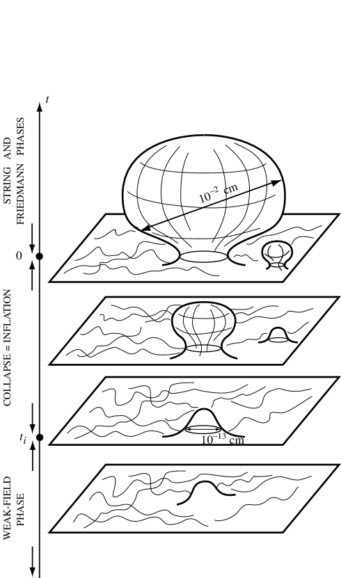
Figure 4:

A basic difference between the large numbers needed in (non-inflationary) FRW cosmology and the large numbers needed in PBB cosmology should be stressed at this point. In the former, the ratio of two classical scales, e.g. of total curvature to its spatial component, which is expected to be $O(1)$, has to be taken as large as $10^{60}$. In the latter, the above ratio is initially $O(1)$ in the collapsing/inflating region, and ends up being very large in that region thanks to DDI. However, the common order of magnitude of these two classical quantities is a free parameter, and is taken to be much larger than a classically irrelevant quantum scale.

We can visualize analogies and differences between standard and pre-big bang inflation by comparing Figs. 5a and 5b. In these, we sketch the evolution of the Hubble radius and of a fixed comoving scale (here the one corresponding to the part of the Universe presently observable to us) as a function of time in the two scenarios. The common feature is that the fixed comoving scale was “inside the horizon” for some time during inflation, and possibly very deeply inside at its onset. Also, in both cases, the Hubble radius at the beginning of inflation had to be large in Planck units and the scale of homogeneity had to be at least as large. The difference between the two scenarios is just in the behaviour of the Hubble radius during inflation: increasing in standard inflation (a), decreasing in string cosmology (b). This is what makes PBB’s “wine glass” more elegant, and stable! Thus, while standard inflation is still facing the initial-singularity question and needs a non-adiabatic phenomenon to reheat the Universe (a kind of small bang), PBB cosmology faces the singularity problem later, combining it to the exit and heating problems (discussed in Sections V and VIB, respectively).

In the end, what saves PBB cosmology from fine-tuning is (not surprisingly!) supersymmetry. This is what protects us from the appearance of a cosmological constant in the weak-coupling regime. Even a relatively small cosmological constant would invalidate our scale-invariance arguments and force DDI to be very short [5]. Thus, amusingly, while an effective cosmological constant is at the basis of standard (post-big bang) inflation, its absence in the weak coupling region is at the basis of PBB inflation. This may allow us to speculate that the absence (or extreme smallness) of the present cosmological constant may be related to a mysterious degeneracy between the perturbative and the non-perturbative vacuum of superstring theory.

5 The exit problem/conjecture

We have argued that, generically, DDI, when studied at lowest order in derivatives and coupling, evolves towards a singularity of the big bang type. Similarly, at the same level of approximation, the non-inflationary solutions emerge from a singularity. Matching these two branches in a smooth, non-singular way has become known as the (graceful) exit problem in string cosmology [14]. It is, undoubtedly, the most important theoretical problem facing the whole PBB scenario.

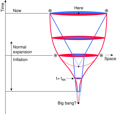
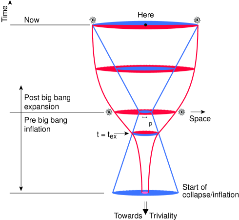
Figure 5:

There has been quite some progress recently on the exit problem. However, for lack of space, I shall refer the reader to the literature [14] for details. Generically speaking, toy examples have shown that DDI can flow, thanks to higher-curvature corrections, into a de-Sitter-like phase, i.e. into a phase of constant $H$ (curvature) and constant $\dot{\phi}$. This phase is expected to last until loop corrections become important (see next section) and give rise to a transition to a radiation-dominated phase. If these toy models serve as an indication, the full exit problem can only be achieved at large coupling and curvature, a situation that should be described by the newly invented M-theory [3].

It was recently pointed out [15] that the reverse order of events is also possible. The coupling may become large before the curvature. In this case, at least for some time, the low-energy limit of M-theory should be adequate: this limit is known [3] to give $D=11$ supergravity and is therefore amenable to reliable study. It is likely, though not yet clear, that, also in this case, strong curvatures will have to be reached before the exit can be completed. In the following, we will assume that:

• the big bang singularity is avoided thanks to the softness of string theory;

• full exit to radiation occurs at strong coupling and curvature, according to a criterion given in Section VIB.

6 Observable relics and heating the pre-bang Universe

6.1 PBB relics

Since there are already several review papers on this subject (e.g. [16]), I will limit myself to mentioning the most recent developments, after recalling the basic physical mechanism underlying particle production in cosmology [17]. A cosmological (i.e. time-dependent) background coupled to a given type of (small) inhomogeneous perturbation $\Psi$ enters the effective low-energy action in the form:

$$I={\small\frac{1}{2}}\int d\eta\ d^{3}x\ S(\eta)\left[\Psi^{\prime 2}-(\nabla\Psi)^{2}\right].$$ (8)

Here $\eta$ is the conformal-time coordinate, and a prime denotes $\partial/\partial\eta$. The function $S(\eta)$ (sometimes called the “pump” field) is, for any given $\Psi$, a given function of the scale factor $a(\eta)$, and of other scalar fields (four-dimensional dilaton $\phi(\eta)$, moduli $b_{i}(\eta)$, etc.), which may appear non-trivially in the background.

While it is clear that a constant pump field $S$ can be reabsorbed in a rescaling of $\Psi$, and is thus ineffective, a time-dependent $S$ couples non-trivially to the fluctuation and leads to the production of pairs of quanta (with equal and opposite momenta). One can easily determine the pump fields for each one of the most interesting perturbations. The result is:

$$\rm{Gravity~{}waves,~{}dilaton} : S=a^{2}e^{-\phi}$$

$$\rm{Heterotic~{}gauge~{}bosons} : S=e^{-\phi}$$

$$\rm{Kalb-Ramond,~{}axions} : S=a^{-2}e^{-\phi}\;.$$ (9)

A distinctive property of string cosmology is that the dilaton $\phi$ appears in some very specific way in the pump fields. The consequences of this are very interesting:

• For gravitational waves and dilatons, the effect of $\phi$ is to slow down the behaviour of $a$ (remember that both $a$ and $\phi$ grow in the pre-big bang phase). This is the reason why those spectra are quite steep [18] and give small contributions at large scales. Thus one of the most robust predictions of PBB cosmology is a small tensor component in the CMB anisotropy. The reverse is also true: at short scales, the expected yield in a stochastic background of gravitational waves is much larger than in standard inflationary cosmology. This is easily understood: in standard inflation the GW spectrum is either flat or slowly decreasing (as a function of frequency). Since COBE data [19] set a limit on the GW contribution at large scales, this bound holds a fortiori at shorter scales, as those of interest for direct GW detection. Thus, in standard inflation, one expects

  $$\Omega_{GW}<10^{-14}\;.$$ (10)

  Since the GW spectra of PBB cosmology are “blue”, the bound by COBE is automatically satisfied, with no implication on the GW yield at interesting frequencies. Values of $\Omega_{GW}$ in the range of $10^{-6}$–$10^{-7}$ are possible in some regions of parameter space, which, according to some estimates of sensitivities [20], could be inside detection capabilities in the near future.

• For gauge bosons there is no amplification of vacuum fluctuations in standard cosmology, since a conformally flat metric (of the type forced upon by inflation) decouples from the electromagnetic (EM) field precisely in $D=3+1$ dimensions. As a very general remark, apart from pathological solutions, the only background field which, through its cosmological variation, can amplify EM (more generally gauge-field) quantum fluctuations is the effective gauge coupling itself [21]. By its very nature, in the pre-big bang scenario the effective gauge coupling inflates together with space during the PBB phase. It is thus automatic that any efficient PBB inflation brings together a huge variation of the effective gauge coupling and thus a very large amplification of the primordial EM fluctuations [22, 23, 24]. This can possibly provide the long-sought origin for the primordial seeds of the observed galactic magnetic fields. Notice, however, that, unlike GW, EM perturbations interact quite considerably with the hot plasma of the early (post-big bang) Universe. Thus, converting the primordial seeds into those that may have existed at the proto-galaxy formation epoch is by no means a trivial exercise. Work is in progress to try to adapt existing codes [25] to the evolution of our primordial seeds.

• Finally, for Kalb–Ramond fields and axions, $a$ and $\phi$ work in the same direction and spectra can be large even at large scales [26]. An interesting fact is that, unlike the GW spectrum, that of axions is very sensitive to the cosmological behaviour of internal dimensions during the DDI epoch. On one side, this makes the model less predictive. On the other, it tells us that axions represent a window over the multidimensional cosmology expected generically from string theories, which must live in more that four dimensions. Curiously enough, the axion spectrum becomes exactly HZ (i.e. scale-invariant) when all the nine spatial dimensions of superstring theory evolve in a rather symmetric way [23]. In situations near this particularly symmetric one, axions are able to provide a new mechanism for generating large-scale CMB anisotropy and LSS.

  A recent calculation [27] of the effect gives, for massless axions,

  $$l(l+1)C_{l}\sim O(1)\left({H_{max}\over M_{P}}\right)^{4}(\eta_{0}k_{max})^{-2\alpha}{\Gamma(l+\alpha)\over\Gamma(l-\alpha)}\;,$$ (11)

  where $C_{l}$ are the usual coefficients of the multipole expansion of $\Delta T/T$

  $$\langle\Delta T/T(\vec{n})~{}~{}\Delta T/T(\vec{n}^{\prime})\rangle~{}=~{}\sum_{l}(2l+1)C_{l}P_{l}(\cos\theta)\;,$$ (12)

  and the parameters $H_{max},k_{max},\alpha$ are defined by the primordial axion energy spectrum in critical units as:

  $$\Omega_{ax}(k)=\left({H_{max}\over M_{P}}\right)^{2}(k/k_{max})^{\alpha}\;.$$ (13)

  In string theory, as repeatedly mentioned, we expect $H_{max}/M_{P}\sim M_{s}/M_{P}\sim 1/10$ and $\eta_{0}k_{max}\sim 10^{30}$, while the exponent $\alpha$ depends on the explicit PBB background with the above-mentioned HZ case corresponding to $\alpha=0$. The standard tilt parameter $n=n_{s}$ ($s$ for scalar) is given by $n=1+2\alpha$ and is found, by COBE, to lie between $0.9$ and $1.5$, corresponding to $0<\alpha<0.25$ (a negative $\alpha$ leads to some theoretical problems). With these inputs we can see that the correct normalization ($C_{2}\sim 10^{-10}$) is reached for $\alpha\sim 0.2$, which is just in the middle of the allowed range. In other words, unlike in standard inflation, we cannot predict the tilt, but when this is given, we can predict (again unlike in standard inflation) the normalization.

  Our model, being of the isocurvature type, bears some resemblance to the one recently advocated by Peebles [28] and, like his, is expected to contain some calculable amount of non-Gaussianity, which is being calculated and will be checked by the future satellite measurements (MAP, PLANCK).

• Many other perturbations, which arise in generic compactifications of superstrings, have also been studied, and lead to interesting spectra. For lack of time, I will refer to the existing literature [23, 24].

6.2 Heat and entropy as a quantum gravitational instability

Before closing this section, I wish to recall how one sees the very origin of the hot big bang in this scenario. One can easily estimate the total energy stored in the quantum fluctuations, which were amplified by the pre-big bang backgrounds. The result is, roughly,

$$\rho_{quantum}\sim N_{eff}~{}H^{4}_{max}\;,$$ (14)

where $N_{eff}$ is the effective number of species that are amplified and $H_{max}$ is the maximal curvature scale reached around $t=0$. We have already argued that $H_{max}\sim M_{s}=\lambda_{s}^{-1}$, and we know that, in heterotic string theory, $N_{eff}$ is in the hundreds. Yet this rather huge energy density is very far from critical, as long as the dilaton is still in the weak-coupling region, justifying our neglect of back-reaction effects. It is very tempting to assume [23] that, precisely when the dilaton reaches a value such that $\rho_{quantum}$ is critical, the Universe will enter the radiation-dominated phase. This PBBB (PBB bootstrap) constraint gives, typically:

$$e^{\phi_{exit}}\sim 1/N_{eff}\;\;,$$ (15)

i.e. a value for the dilaton close to its present value.

The entropy in these quantum fluctuations can also be estimated following some general results [29]. The result for the density of entropy $S$ is, as expected

$$S\sim N_{eff}H_{max}^{3}\;.$$ (16)

It is easy to check that, at the assumed time of exit given by (15), this entropy saturates a recently proposed holography bound [30]. This also turns out to be a physically acceptable value for the entropy of the Universe just after the big bang: a large entropy on the one hand (about $10^{90}$); a small entropy for the total mass and size of the observable Universe on the other, as often pointed out by Penrose [31]. Thus, PBB cosmology neatly explains why the Universe, at the big bang, looks so fine-tuned (without being so) and provides a natural arrow of time in the direction of higher entropy.

7 Conclusions

• Pre-big bang (PBB) cosmology is a “top–down” rather than a “bottom–up” approach to cosmology. This should not be forgotten when testing its predictions.

• It does not need to invent an inflaton, or to fine-tune its potential; inflation is “natural” thanks to the duality symmetries of string cosmology.

• It makes use of a classical gravitational instability to inflate the Universe, and of a quantum instability to warm it up.

• The problem of initial conditions “decouples” from the singularity problem; it is classical, scale-free, and unambiguously defined. Issues of fine tuning can be addressed and, I believe, answered.

• The spectrum of large-scale perturbations has become more promising through the invisible axion of string theory, while the possibility of explaining the seeds of galactic magnetic fields remains a unique prediction of the model.

• The main conceptual (technical?) problem remains that of providing a fully convincing mechanism for (and a detailed description of) the pre-to-post-big bang transition. It is very likely that such a mechanism will involve both high curvatures and large coupling and should therefore be discussed in the (yet to be fully constructed) M-theory [3]. New ideas borrowed from such theory and from D-branes [32, 15] could help in this respect.

• Once/if this problem will be solved, predictions will become more precise and robust, but, even now, with some mild assumptions, several tests are (or will soon become) possible, e.g.

  • the tensor contribution to $\Delta T/T$ should be very small (see, however, footnote Section VI);

  • some non-Gaussianity in $\Delta T/T$ correlations is expected, and calculable.

  • the axion-seed mechanism should lead to a characteristic acoustic-peak structure, which is being calculated;

  • it should be possible to convert the predicted seed magnetic fields into observables by using some reliable code for their late evolution;

  • a characteristic spectrum of stochastic gravitational waves is expected to surround us and could be large enough to be measurable within a decade or so.

References

- [1] E. W. Kolb and M. S. Turner, The Early Universe (Addison-Wesley, Redwood City, CA, 1990); A.D. Linde, Particle Physics and Inflationary Cosmology (Harwood, New York, 1990).
- [2] G. Veneziano, Europhys. Lett. 2 (1986) 133; The Challenging Questions, Erice, 1989, ed. A. Zichichi (Plenum Press, New York, 1990), p. 199.
-
[3]
See, e.g., E. Witten, Nucl. Phys. B443 (1995) 85;
P. Horawa and E. Witten, Nucl. Phys. B460 (1996) 506. - [4] T.R. Taylor and G. Veneziano, Phys. Lett. B213 (1988) 459.
- [5] G. Veneziano, Phys. Lett. B265 (1991) 287.
- [6] M. Gasperini and G. Veneziano, Astropart. Phys. 1 (1993) 317, Mod. Phys. Lett. A8 (1993) 3701, Phys. Rev. D50 (1994) 2519.
- [7] An updated collection of papers on the PBB scenario is available at http://www.to.infn.it/~gasperin/.
- [8] A. Buonanno, T. Damour and G. Veneziano, Pre-big bang bubbles from the gravitational instability of generic string vacua, hep-th/9806230; see also, G. Veneziano, Phys. Lett. B406 (1997) 297; A. Buonanno, K.A. Meissner, C. Ungarelli and G. Veneziano, Phys. Rev. D57 (1998) 2543, and references therein.
-
[9]
R. Penrose, Structure of space-time, in Battelle Rencontres,
ed. C. Dewitt and
J.A. Wheeler, Benjamin, New York, 1968. - [10] D. Christodoulou, Commun. Pure Appl. Math. 56 (1993) 1131, and references therein.
- [11] R. Penrose, Phys. Rev. Lett. 14 (1965) 57; S. W. Hawking and R. Penrose, Proc. Roy. Soc. Lond. A314 (1970) 529.
- [12] M. Turner and E. Weinberg, Phys. Rev. D56 (1997) 4604; N. Kaloper, A. Linde and R. Bousso, Pre-big bang requires the Universe to be exponentially large from the very beginning, hep-th/9801073.
- [13] A. Linde, Phys. Lett. 129B (1983) 177.
- [14] R. Brustein and G. Veneziano, Phys. Lett. B329 (1994) 429; N. Kaloper, R. Madden and K.A. Olive, Nucl. Phys. B452 (1995) 677, Phys. Lett. B371 (1996) 34; R. Easther, K. Maeda and D. Wands, Phys. Rev. D53 (1996) 4247; M. Gasperini, M. Maggiore and G. Veneziano, Nucl. Phys. B494 (1997) 315; R. Brustein and R. Madden, Phys. Lett. B410 (1997) 110, Phys. Rev. D57 (1998) 712.
-
[15]
M. Maggiore and A. Riotto, D-branes and Cosmology, hep-th/9811089;
see also T. Banks, W. Fishler and L. Motl, Duality versus Singularities, hep-th/9811194. - [16] G. Veneziano, in String Gravity and Physics at the Planck Energy Scale, Erice, 1995, eds. N. Sanchez and A. Zichichi (Kluver Academic Publishers, Boston, 1996), p. 285; M. Gasperini, ibid., p. 305.
- [17] See, e.g., V. F. Mukhanov, A. H. Feldman and R. H. Brandenberger, Phys. Rep. 215 (1992) 203.
- [18] R. Brustein, M. Gasperini, M. Giovannini and G. Veneziano, Phys. Lett. B361 (1995) 45; R. Brustein et al., Phys. Rev. D51 (1995) 6744.
- [19] G. F. Smoot et al., Ap. J. 396 (1992) L1; C. L. Bennet et al., Ap. J. 430 (1994) 423.
- [20] P. Astone et al., Phys. Lett. B385 (1996) 421; B. Allen and R. Brustein, Phys. Rev. D55 (1997) 970.
- [21] B. Ratra, Astrophys. J. Lett. 391 (1992) L1.
-
[22]
M. Gasperini, M. Giovannini and G. Veneziano, Phys. Rev. Lett. 75 (1995) 3796;
D. Lemoine and M. Lemoine, Phys. Rev. D52 (1995) 1955. - [23] A. Buonanno, K. A. Meissner, C. Ungarelli and G. Veneziano, JHEP 1 (1998) 4;
- [24] R. Brustein and M. Hadad, Phys. Rev. D57 (1998) 725.
- [25] R. M. Kulsrud, R. Cen, J. P. Ostriker and D. Ryu, Ap. J. 480 (1997) 481.
- [26] E.J. Copeland, R. Easther and D. Wands, Phys. Rev. D56 (1997) 874; E.J. Copeland, J.E. Lidsey and D. Wands, Nucl. Phys. B506 (1997) 407.
- [27] R. Durrer, M. Gasperini, M. Sakellariadou and G. Veneziano, Phys. Lett. B436 (1998) 66, Phys. Rev. D59 (1999) 043511; M. Gasperini and G. Veneziano, Phys. Rev. D59 (1999) 043503.
- [28] P. J. E. Peebles, An isocurvature CDM cosmogony. I and II, astro-ph/9805194, and astro-ph/9805212.
- [29] M. Gasperini and M. Giovannini, Phys. Lett. B301 (1993) 334; Class. Quant. Grav. 10 (1993) L133; R. Brandenberger, V. Mukhanov and T. Prokopec, Phys. Rev. Lett. 69 (1992) 3606; Phys. Rev. D48 (1993) 2443.
-
[30]
W. Fischler and L. Susskind, Holography and Cosmology, hep-th/9806039;
see also
D. Bak and S.-J. Rey, Holographic principle and string cosmology, hep-th/9811008;
A. K. Biswas, J. Maharana and R.K. Pradhan, The holography principle and pre-big bang cosmology, hep-th/9811051. - [31] see, e.g., R. Penrose, The Emperor’s new mind, (Oxford University Press, New York, 1989), Chapter 7.
- [32] A. Lukas, B.A. Ovrut and D. Waldram, Phys. Lett. B393 (1997) 65; Nucl. Phys. B495 (1997) 365; F. Larsen and F. Wilczek, Phys. Rev. D55 (1997) 4591; N. Kaloper, Phys. Rev. D55 (1997) 3394; H. Lu, S. Mukherji and C.N. Pope, Phys. Rev. D55 (1997) 7926; R. Poppe and S. Schwager, Phys. Lett. B393 (1997) 51; A. Lukas and B. A. Ovrut, Phys. Lett. B437 (1998) 291; N. Kaloper, I. Kogan and K. A. Olive, Phys. Rev. D57 (1998) 7340.