Quantum Field Theory in a Topology Changing Universe

Abstract

We propose a method to construct quantum theory of matter fields in a topology changing universe. Analytic continuation of the semiclassical gravity of a Lorentzian geometry leads to a non-unitary Schrödinger equation in a Euclidean region of spacetime, which does not have a direct interpretation of quantum theory of the Minkowski spacetime. In this Euclidean region we quantize the Euclidean geometry, derive the time-dependent Schrödinger equation and find the quantum states using the Liouville-Neumann method. The Wick rotation of these quantum states provides the correct Hilbert space of matter field in the Euclidean region of the Lorentzian geometry. It is found that the direct quantization of a scalar field in the Lorentzian geometry involves an unusual commutation rule in the Euclidean region. Finally we discuss the interpretation of the periodic solution of the semiclassical gravity equation in the Euclidean geometry as a finite temperature solution for the gravity-matter system in the Lorentzian geometry.

I Introduction

The open inflation model proposed recently by Hawking-Turok [1] revived an interest in the wave functions of quantum cosmology, and provoked a debate on the boundary conditions of the Universe [2]. The present Lorentzian spacetime is supposed to emerge quantum mechanically from a Euclidean spacetime. Leading proposals for such wave functions are the Hartle-Hawking’s no-boundary wave function [3], the Linde’s wave function [4] and the Vilenkin’s tunneling wave function [5]. Though there has not still been an unanimous agreement on the boundary condition of the Universe, it is generally accepted that the Universe which tunneled quantum mechanically the Euclidean spacetime should have either an exponentially growing or decaying wave function or a combination of both branches [6]. But the issue of quantum theory of matter fields in a topology changing universe such as the tunneling universe has not been raised seriously yet.

It is the purpose of this paper to investigate a consistent quantum theory of a scalar field in the Euclidean region of the topology changing universe such as the tunneling universe and to construct quantum states explicitly there. To treat the quantum field in a curved spacetime there have been used two typical methods: in the conventional approach the underlying spacetime is fixed as a background and matter field is quantized on it [7], and in the other approach known as the semiclassical (quantum) gravity the semiclassical Einstein equation with the quantum back-reaction of matter field and the time-dependent Schrödinger equation are derived from the Wheeler-DeWitt equation for the gravity-matter system [8, 9, 10, 11]. In both approaches the functional Schrödinger equation for the scalar field in the Euclidean region obeys a non-unitary (diffusion-like) evolution equation. So the quantization rules of the Minkowski spacetime may not be applied directly. To construct the consistent quantum theory in the Euclidean region we propose a method in which one first quantizes the Wick-rotated gravity-matter system of the Euclidean geometry, derives the time-dependent Schrödinger equation and then transforms back via the Wick rotation the quantum states into those of the Lorentzian geometry. This method is consistent because the Wick rotations are well defined and so does the time-dependent Schrödinger equation in the Euclidean region in the Euclidean geometry just as in the Lorentzian region of the Lorentzian geometry. It is also useful in that one is able to find the quantum states explicitly using the Liouville-Neumann method which has already been used to find quantum states of the scalar field in the Lorentzian regions of spacetime [12].

The organization of the paper is as follows. In Sec. II we quantize the gravity-scalar system in the Lorentzian geometry and derive the semiclassical Einstein equation and the time-dependent Schrödinger equation from the Wheeler-DeWitt equation in the Lorentzian region where the gravitational wave function oscillates. The region where the gravitational wave function exhibits an exponential behavior corresponds to a Euclidean region of spacetime. We focus in particular on the Schrödinger equation in the Euclidean region of spacetime. In Sec. III we quantize the Euclidean gravity (geometry) coupled to the minimal scalar field and derive the time-dependent Schrödinger equation together with the semiclassical Einstein equation in the region corresponding to the Euclidean region of the Lorentzian geometry. Quantum states are found using the Liouville-Neumann method. In Sec. IV the Wick rotation is employed to transform these quantum states defined in terms of the Euclidean geometry into those defined in terms of the Lorentzian geometry.

II Quantum Theory in Lorentzian Geometry

As a simple but interesting quantum cosmological model, let us consider the closed FRW universe minimally coupled to an inflaton, a minimal scalar field. The action for the gravity with a cosmological constant $\Lambda$ and the scalar field takes the form

$$I=\frac{m_{P}^{2}}{16\pi}\int d^{4}x\sqrt{-g}\Bigl{[}R-2\Lambda\Bigr{]}+\frac{m_{P}^{2}}{8\pi}\int d^{3}x\sqrt{h}K+\int d^{4}x\sqrt{-g}\Bigl{[}\frac{1}{2}g^{\mu\nu}\partial_{\mu}\phi\partial_{\nu}\phi-V(\phi)\Bigr{]},$$ (1)

where $m_{P}^{2}=1/G$ is the Planck mass squared. The surface term for the gravity has been introduced to yield the correct Einstein equation for the closed universe. In the Lorentzian FRW universe with the metric in the ADM formulation

$$ds^{2}_{L}=-N^{2}(t)dt^{2}+a^{2}(t)d\Omega_{3}^{2},$$ (2)

the action becomes

$$I_{L}=\int dt\Biggl{[}-\frac{3\pi m_{P}^{2}}{4}\Biggl{(}\frac{a}{N}\Bigl{(}\frac{\partial a}{\partial t}\Bigr{)}^{2}-NV_{g}(a)\Biggr{)}+2\pi^{2}a^{3}\Biggl{(}\frac{1}{2N}\Bigl{(}\frac{\partial\phi}{\partial t}\Bigr{)}^{2}-NV(\phi)\Biggr{)}\Biggr{]},$$ (3)

where

$$V_{g}(a)=a-\frac{\Lambda}{3}a^{3}.$$ (4)

In the above equation we dropped the second order derivative term, which is to be cancelled by a boundary action. By introducing the canonical momenta

$$\pi_{a}=-\frac{3\pi m_{P}^{2}a}{2\pi N}\frac{\partial a}{\partial t},~{}\pi_{\phi}=\frac{2\pi^{2}a^{3}}{N}\frac{\partial\phi}{\partial t},$$ (5)

one obtains the Hamiltonian constraint

$${\cal H}_{L}=\hat{H}_{g}(\pi_{a},a)+\hat{H}_{L}(\pi_{\phi},\phi,a)=0,$$ (6)

where

$$\hat{H}_{g}(\pi_{a},a) = -\frac{1}{3\pi m_{P}^{2}a}\pi_{a}^{2}-\frac{3\pi m_{P}^{2}}{4}V_{g}(a),$$ (7)

$$\hat{H}_{L}(\pi_{\phi},\phi,a) = \frac{1}{4\pi^{2}a^{3}}\pi_{\phi}^{2}+2\pi^{2}a^{3}V(\phi)$$ (8)

are the Hamiltonians for the gravity and scalar field, respectively. The Dirac quantization leads to the Wheeler-DeWitt equation for the Lorentzian geometry

$$\Biggl{[}-\frac{\hbar^{2}}{3\pi m_{P}^{2}a}\frac{\partial^{2}}{\partial a^{2}}+\frac{3\pi m_{P}^{2}}{4}V_{g}(a)+\frac{\hbar^{2}}{4\pi^{2}a^{3}}\frac{\partial^{2}}{\partial{\phi}^{2}}-2\pi^{2}a^{3}V(\phi)\Biggr{]}\Psi_{L}(a,\phi)=0,$$ (9)

where we neglected the operator ordering ambiguity.

Before we derive the equation for quantum fields in the Euclidean region, we review briefly how to obtain the time-dependent Schrödinger equation in the Lorentzian region from the semiclassical (quantum) gravity point of view. In the Lorentzian region, where the wave function for the gravitational field oscillates, we first adopt the Born-Oppenheimer idea to expand the total wave function according to different mass scales

$$\Psi_{L}(a,\phi)=\psi_{L}(a)\Phi_{L}(\phi,a),$$ (10)

and obtain the gravitational field equation with the back-reaction of matter field [10]

$$\Biggl{[}-\frac{\hbar^{2}}{3\pi m_{P}^{2}a}D^{2}+\frac{3\pi m_{P}^{2}}{4}V_{g}(a)+\langle\hat{H}_{L}\rangle-\frac{\hbar^{2}}{3\pi m_{P}^{2}a}\langle\bar{D}^{2}\rangle\Biggr{]}\psi_{L}(a)=0.$$ (11)

Here, $D$ and $\bar{D}$ denote the covariant derivatives

$$D=\frac{\partial}{\partial a}+iA(a),~{}~{}\bar{D}=\frac{\partial}{\partial a}-iA(a),$$ (12)

with an effective gauge potential from the scalar field

$$A(a)=-i\frac{\langle\Phi_{L}|\frac{\partial}{\partial a}|\Phi_{L}\rangle}{\langle\Phi_{L}|\Phi_{L}\rangle},$$ (13)

and $\langle\hat{H}_{L}\rangle$ and $\langle\bar{D}^{2}\rangle$ denote the expectation value of the corresponding operators

$$\langle\hat{H}_{L}\rangle=\frac{\langle\Phi_{L}|\hat{H}_{L}|\Phi_{L}\rangle}{\langle\Phi_{L}|\Phi_{L}\rangle},~{}~{}\langle\bar{D}^{2}\rangle=\frac{\langle\Phi_{L}|\hat{H}_{L}|\Phi_{L}\rangle}{\langle\Phi_{L}|\Phi_{L}\rangle}.$$ (14)

By putting Eq. (10) into Eq. (9) and by subtracting Eq. (11), one gets the equation for the matter field

$$-\frac{2\hbar^{2}}{3\pi m_{P}^{2}a}\frac{1}{\psi_{L}}\bigl{(}D\psi_{L}\bigr{)}\bigl{(}\bar{D}\Phi_{L}\bigr{)}+\bigl{(}\hat{H}_{L}-\langle\hat{H}_{L}\rangle\bigr{)}\Phi_{L}-\frac{\hbar^{2}}{3\pi m_{P}^{2}a}\bigl{(}\bar{D}^{2}-\langle\bar{D}^{2}\rangle\bigr{)}\Phi_{L}=0.$$ (15)

Since $A(a)$ is a gauge potential and a $c$-number, the geometric phases for the wave function and quantum state

$$\psi_{L}(a)=e^{-i\int A}\tilde{\psi}_{L},~{}~{}\Phi_{L}=e^{i\int A}\tilde{\Phi}_{L},$$ (16)

remove the gauge potentials from the covariant derivatives $D$ and $\bar{D}$, in Eqs. (11) and (15). However, the total wave function (10) keeps the same form $\Psi_{L}=\tilde{\psi}_{L}\tilde{\Phi}_{L}$. From now on we shall work with the wave function and quantum state (16), drop the tildes for simplicity and ignore the last terms in Eqs. (11) and (15), which are small compared with the other terms.

We then follow the de Broglie-Bohm interpretation and set the gravitational wave function in the form

$$\psi_{L(II)}(a)=F(a)\exp\Bigl{[}\pm\frac{i}{\hbar}S_{L(II)}(a)\Bigr{]},$$ (17)

Here, $(II)$ denotes an oscillatory region of Lorentzian geometry (see Fig.1) and $\pm$ signs correspond to the expanding and collapsing branches of the universe, respectively. The real part gives rise to the Hamilton-Jacobi equation

$$\frac{1}{3\pi m_{P}^{2}a}\Bigl{(}\frac{\partial S_{L(II)}}{\partial a}\Bigr{)}^{2}+\frac{3\pi m_{P}^{2}}{4}V_{g}-\frac{1}{3\pi m_{P}^{2}a}V_{q}-\langle\hat{H}_{m}\rangle=0,$$ (18)

where

$$V_{q}(a)=\hbar^{2}\frac{\partial^{2}F/\partial a^{2}}{F}$$ (19)

is the quantum potential. The imaginary part leads to the continuity equation

$$F\frac{\partial^{2}S_{L(II)}}{\partial a^{2}}+2\frac{\partial F}{\partial a}\frac{\partial S_{L(II)}}{\partial a}=0.$$ (20)

The contribution $V_{q}$ from the quantum potential will also be ignored, which is at most one-loop or higher orders. By integrating $c$-number $\langle\hat{H}_{L}\rangle$ and writing it as a phase factor of $\Phi_{L}=e^{i\int\langle\hat{H}_{L}\rangle}\tilde{\tilde{\Phi}}_{L}$ in Eq. (15) and once again dropping the tilde for simplicity, one also obtains the time-dependent Schrödinger equation for the scalar field

$$i\hbar\frac{\partial}{\partial t}\Phi_{L}(\phi,t)=\hat{H}_{L}\Bigl{(}\frac{\hbar}{i}\frac{\partial}{\partial\phi},\phi,t\Bigr{)}\Phi_{L}(\phi,t),$$ (21)

where $t$ is the cosmological (WKB) time

$$\frac{\partial}{\partial t}=\mp\frac{2}{3\pi m_{P}^{2}a}\frac{\partial S_{L(II)}}{\partial a}\frac{\partial}{\partial a}.$$ (22)

By identifying the cosmological time (22) with the comoving time in Eq. (2) and by making use of

$$\frac{\partial S_{L(II)}}{\partial a}=\mp\frac{3\pi m_{P}^{2}a}{2}\frac{\partial a}{\partial t},$$ (23)

one sees that Eq. (18) becomes indeed the semiclassical Einstein equation

$$\Biggl{(}\frac{\frac{\partial a}{\partial t}}{a}\Biggr{)}^{2}+\frac{1}{a^{2}}-\frac{\Lambda}{3}=\frac{4}{3\pi m_{P}^{2}a^{3}}\langle\hat{H}_{L}\rangle.$$ (24)

The spacetime regions are divided according as the effective potential for the gravitational field

$$V_{L}(a)=\frac{3\pi m_{P}^{2}}{4}V_{g}(a)-\langle\hat{H}_{L}\rangle$$ (25)

takes positive or negative values. For the sake of simplicity, we assume that the quantum back-reaction of the scalar field is insignificant compared with $V_{g}$, so that the effective potential $V_{L}$ has a simple form in Fig. 1. The region I of Fig. 1, where $V_{L}$ is positive, corresponds to a part of Euclidean spacetime, whereas the region II, where $V_{L}$ is negative, corresponds to a part of Lorentzian spacetime.

Being mostly interested in the quantum creation of the universe from the Euclidean region of the tunneling universe to the Lorentzian region, we focus on the region I of Fig. 1. Though the gravitational motion is prohibited classically in the region I, it is, however, permitted quantum mechanically. In this region one is tempted to continue analytically the wave function (17) to get

$$\psi_{L(I)}(a)=F(a)\exp\Bigl{[}\mp\frac{1}{\hbar}S_{L(I)}(a)\Bigr{]},$$ (26)

whose dominant contribution to Eq. (11) leads to the Hamilton-Jacobi-like equation

$$\Bigl{(}\frac{\partial S_{L(I)}}{\partial a}\Bigr{)}^{2}=3\pi m_{P}^{2}aV_{L}.$$ (27)

At the same time one is able to obtain from Eq. (15) the time-dependent Schrödinger equation

$$\hbar\frac{\partial}{\partial s}\Phi_{L}(\phi,s)=\hat{H}_{L}\Bigl{(}\frac{\hbar}{i}\frac{\partial}{\partial\phi},\phi,s\Bigr{)}\Phi_{L}(\phi,s),$$ (28)

where $s$ is a Euclidean analog of cosmological time defined by

$$\frac{\partial}{\partial s}=\pm\frac{2}{3\pi m_{P}^{2}a}\frac{\partial S_{L(I)}}{\partial a}\frac{\partial}{\partial a}.$$ (29)

But the scalar field Hamiltonian $\hat{H}_{L}$ keeps the same form.

Then the following questions are raised. What is the meaning of the parameter $s$? Is it an analytic continuation of the cosmological time or a Wick-rotated Euclidean time? How to solve Eq. (28), an apparently time-dependent diffusion-like equation? What are the quantization rule $\bigl{[}\hat{\phi},\hat{\pi}_{\phi}\bigr{]}$ and the meaning of quantum states of this non-unitary evolution? To answer these questions and to follow analogy with quantum theory of Lorentzian spacetime, we shall consider the quantum theory of the scalar field by quantizing the Euclidean geometry.

III Quantum Theory in Euclidean Geometry

To obtain the quantum cosmological model for the Euclidean spacetime, we perform the Wick rotation $t=i\tau$ and consider the Euclidean metric

$$ds^{2}=N^{2}(\tau)d\tau^{2}+a^{2}(\tau)d\Omega^{2}_{3}.$$ (30)

From the Euclidean action

$$I_{E}=\int d\tau\Biggl{[}\frac{3\pi m_{P}^{2}}{4}\Biggl{(}\frac{a}{N}\Bigl{(}\frac{\partial a}{\partial\tau}\Bigr{)}^{2}+NV_{g}(a)\Biggr{)}-2\pi^{2}a^{3}(\tau)\Biggl{(}\frac{1}{2N}\Bigl{(}\frac{\partial\phi}{\partial\tau}\Bigr{)}^{2}+NV(\phi)\Biggr{)}\Biggr{]},$$ (31)

we obtain the Hamiltonian constraint

$${\cal H}_{E}=\frac{1}{3\pi m_{P}^{2}a}\pi_{E,a}^{2}-\frac{3\pi m_{P}^{2}}{4}V_{g}(a)-\frac{1}{4\pi^{2}a^{3}}\pi_{E,\phi}^{2}+2\pi^{2}a^{3}V(\phi)=0,$$ (32)

where

$$\pi_{E,a}=\frac{3\pi m_{P}^{2}a}{2N}\frac{\partial a}{\partial\tau},~{}\pi_{E,\phi}=-\frac{2\pi^{2}a^{3}}{N}\frac{\partial\phi}{\partial\tau}.$$ (33)

The Hamiltonian constraint (32) leads to the Wheeler-DeWitt equation for the Euclidean geometry

$$\Biggl{[}-\frac{\hbar^{2}}{3\pi m_{P}^{2}a}\frac{\partial^{2}}{\partial a^{2}}-\frac{3\pi m_{P}^{2}}{4}V_{g}(a)+\frac{\hbar^{2}}{4\pi^{2}a^{3}}\frac{\partial^{2}}{\partial{\phi}^{2}}+2\pi^{2}a^{3}V(\phi)\Biggr{]}\Psi_{E}(a,\phi)=0.$$ (34)

It should be remarked that the Wick rotation changed both signs of the kinetic terms of the scalar and gravitational fields. This is the reason why the Euclidean action can not be made positive definite for the gravity-matter system.

We now wish to obtain the semiclassical Einstein equation and the time-dependent Schrödinger equation in the Euclidean region I of Fig. 1. Since the sign of the kinetic term of gravitational field was reversed due to the Wick rotation, the wave function $\Psi_{E}$ of the Wheeler-DeWitt equation (34) now oscillates in the region I. This is in contrast with the behavior of the wave function $\Psi_{L}$. Thus we may use the semiclassical quantum gravity approach in Sec. II and Ref. [11]. As in the Lorentzian spacetime we may expand the total wave function in the form of Eq. (10) and set the wave function for the gravity in the form

$$\psi_{E}(a)=F(a)\exp\Bigl{[}\pm\frac{i}{\hbar}S_{E}(a)\Bigr{]}.$$ (35)

The real part of the resultant gravitational field equation, which is similar to Eq. (11) with the reversed signs for both kinetic terms, gives rise to the Hamilton-Jacobi equation

$$\frac{1}{3\pi m_{P}^{2}a}\Bigl{(}\frac{\partial S_{E}}{\partial a}\Bigr{)}^{2}-\frac{3\pi m_{P}^{2}}{4}V_{g}+\langle\hat{H}_{E}\rangle=0,$$ (36)

where

$$\hat{H}_{E}=\frac{\hbar^{2}}{4\pi^{2}a^{3}}\frac{\partial^{2}}{\partial{\phi}^{2}}+2\pi^{2}a^{3}V(\phi)$$ (37)

is the scalar field Hamiltonian in the Euclidean geometry. As in the Lorentzian geometry, one can get the semiclassical Einstein equation in the Euclidean geometry

$$\Biggl{(}\frac{\frac{\partial a}{\partial\tau}}{a}\Biggr{)}^{2}-\frac{1}{a^{2}}+\frac{\Lambda}{3}=-\frac{4}{3\pi m_{P}^{2}a^{3}}\langle\hat{H}_{E}\rangle.$$ (38)

We note that the Euclidean region I corresponds to the region where the effective potential for the gravitational field

$$V_{E}(a)=\frac{3\pi m_{P}^{2}}{4}V_{g}-\langle\hat{H}_{E}\rangle$$ (39)

takes positive values. To consolidate this point further, let us remind that $\langle\hat{H}_{E}\rangle$ is a Wick rotation of $\langle\hat{H}_{L}\rangle$, as will be shown later. So the region where $V_{E}$ is positive, coincides with the region I where $V_{L}$ is positive, too. However, the wave function for the quantized Euclidean geometry oscillates in this region, in contrast with the exponential behavior of the wave function for the quantized Lorentzian geometry. Therefore, we are able to obtain the time-dependent unitary Schrödinger equation

$$i\hbar\frac{\partial}{\partial\tau}\Phi_{E}(\phi,\tau)=\hat{H}_{E}\Bigl{(}\frac{\hbar}{i}\frac{\partial}{\partial\phi},\phi,\tau\Bigr{)}\Phi_{E}(\phi,\tau),$$ (40)

where $\tau$ is the cosmological time defined as

$$\frac{\partial}{\partial\tau}=\mp\frac{2}{3\pi m_{P}^{2}a}\frac{\partial S_{E}}{\partial a}\frac{\partial}{\partial a}.$$ (41)

The cosmological time (41) coincides with the Euclidean time in Eq. (30).

Finally we turn to the task to find quantum states of the scalar field obeying Eq. (40) explicitly. In Ref. [12] the Liouville-Neumann method has been used to construct the Hilbert spaces for quantum inflatons in the FRW background exactly for a quadratic potential and approximately for a generic potential. Similarly we look for the operators that satisfy the Liouville-Neumann equation

$$i\hbar\frac{\partial}{\partial\tau}\left\{\matrix{\hat{A}^{\dagger}\cr\hat{A}\cr}\right\}+\left[\left\{\matrix{\hat{A}^{\dagger}\cr\hat{A}\cr}\right\},\hat{H}_{E}\right]=0.$$ (42)

Two independent Liouville-Neumann operators are found

$$\hat{A}^{\dagger}(\tau) = -i\Bigl{(}\varphi_{E}(\tau)\hat{\pi}_{\phi}-a^{3}(\tau)\frac{\partial\varphi_{E}(\tau)}{\partial\tau}\hat{\phi}\Bigr{)},$$ (43)

$$\hat{A}(\tau) = i\Bigl{(}\varphi^{*}_{E}(\tau)\hat{\pi}_{\phi}-a^{3}(\tau)\frac{\partial\varphi^{*}_{E}(\tau)}{\partial\tau}\hat{\phi}\Bigr{)},$$ (44)

where $\varphi_{E}$ is a complex solution to the equation

$$\frac{\partial^{2}\varphi_{E}(\tau)}{\partial\tau^{2}}+3\Bigl{(}\frac{\partial a(\tau)/\partial\tau}{a(\tau)}\Bigr{)}\frac{\partial\varphi_{E}(\tau)}{\partial\tau}-\frac{\delta^{2}V(\hat{\phi})}{\delta\hat{\phi}^{2}}\varphi_{E}(\tau)=0.$$ (45)

Gaussian states are obtained by taking the expectation value of Eq. (45) with respect to the ground state defined by $\hat{A}(\tau)|0(\tau)\rangle=0$, and by solving the following equation

$$\frac{\partial^{2}\varphi_{E}(\tau)}{\partial\tau^{2}}+3\Bigl{(}\frac{\partial a(\tau)/\partial\tau}{a(\tau)}\Bigr{)}\frac{\partial\varphi_{E}(\tau)}{\partial\tau}-\langle 0(\tau)|\frac{\delta^{2}V(\hat{\phi})}{\delta\hat{\phi}^{2}}|0(\tau)\rangle\varphi_{E}(\tau)=0.$$ (46)

It should be noted that Eq. (45) can also be obtained by the Wick rotation of the Lorentzian equation

$$\frac{\partial^{2}\varphi_{L}(t)}{\partial t^{2}}+3\Bigl{(}\frac{\partial a(t)/\partial t}{a(t)}\Bigr{)}\frac{\partial\varphi_{L}(t)}{\partial t}+\frac{\delta^{2}V(\hat{\phi})}{\delta\hat{\phi}^{2}}\varphi_{L}(t)=0.$$ (47)

Note also that the inverted potential in Eq. (46) can be obtained through mean-field approximation and Wick rotation of the Heisenberg equation of motion in the Lorentzian region

$$\frac{\partial^{2}\hat{\phi}_{L}}{\partial t^{2}}+3\Bigl{(}\frac{\partial a(t)/\partial t}{a(t)}\Bigr{)}\frac{\partial\hat{\phi}_{L}(t)}{\partial t}+\frac{\delta V(\hat{\phi}_{L})}{\delta\hat{\phi}_{L}}=0.$$ (48)

All these aspects are expected in the Wick rotation of quantum theory in the Minkowski spacetime.

IV Transformation between Lorentzian and Euclidean Quantum Geometries

In the tunneling universe of Fig. 1, the Lorentzian geometry is sewn to the Euclidean geometry. There should be a matching condition or surgery of two geometries. Classically to match smoothly across the boundary the extrinsic curvature should be continuous across the boundary. In the FRW universe where the Lorentzian spacetime is connected to the Euclidean spacetime, the extrinsic curvature is given by $\pi_{a}$. We also require that the geometric quantities $a,\pi_{a}$ and physical quantities $\phi,\pi_{\phi}$ be continuous. Sometimes all these are meant the continuity of wave function of the Wheeler-DeWitt equation across the boundary just as the wave function of a quantum mechanical system is continuous across the boundary of tunneling barrier. Though tempted to continue analytically Eq. (18) to describe quantum theory in the Euclidean region, we have seen that such a prescription does not provide a good picture for quantum theory particularly for a gravity-matter system.

In the quantum Lorentzian geometry, the quantum theory of the scalar field in the Euclidean region I is defined in an ad hoc manner via the non-unitary Schrödinger equation. Besides, the quantum operators $\hat{\pi}_{\phi}$ and $\hat{\phi}$, and all the quantization rules are defined in the exactly same manner as in Lorentzian region. This is not obviously a Wick-rotation. On the other hand, in the quantum Euclidean geometry the oscillatory behavior of the Wheeler-DeWitt equation in the same region I enables one to apply the semiclassical quantum gravity approach to obtain a well-defined quantum theory of the scalar field. To get a quantum picture for the scalar field in the Euclidean region there should be a transformation of the Hilbert space constructed in the quantum Euclidean geometry into that of the quantum Lorentzian geometry.

In the de Broglie-Bohm interpretation the canonical momenta are related to the actions

$$\pi_{a}=\frac{\partial S_{L(II)}}{\partial a},~{}\pi_{E,a}=\frac{\partial S_{E}}{\partial a}.$$ (49)

$\pi_{a}$ is well defined in the region II $(a\geq a_{0})$, since

$$\bigl{(}\pi_{a}\bigr{)}^{2}=-3\pi m_{P}^{2}aV_{L}(a)\geq 0,$$ (50)

whereas $\pi_{E,a}$ is well defined in the region I $(a\leq a_{0})$, since

$$\bigl{(}\pi_{E,a}\bigr{)}^{2}=3\pi m_{P}^{2}aV_{E}(a)\geq 0.$$ (51)

To find the momentum $\pi_{a}$ of the Lorentzian geometry in the Euclidean region I we transform back $\pi_{E,a}$ by the inverse Wick rotation $\tau=-is$. Hence, momenta in the Lorentzian and Euclidean geometries are related by the following transformations

$$\pi_{E,a} = i\pi_{a},$$ (52)

$$\pi_{E,\phi} = i\pi_{\phi}.$$ (53)

By making use of Eqs. (49) and (53) we recover the gravitational field wave function (26) of the Lorentzian geometry from that of the Euclidean geometry:

$$\Psi_{E}(a)=F(a)\exp\Bigl{[}\pm\frac{i}{\hbar}S_{E}(a)\Bigr{]}\Rightarrow\Psi_{L}(a)=F(a)\exp\Bigl{[}\mp\frac{1}{\hbar}S_{L(I)}(a)\Bigr{]}.$$ (54)

We turn to the transformation of quantum states of the scalar field. In the region II the scalar field has the energy expectation value with respect to the symmetric Gaussian state $\langle\hat{\phi}\rangle=\phi_{c}=0$

$$\langle\hat{H}_{L}\rangle=\pi^{2}\hbar^{2}a^{3}\frac{\partial\varphi_{L(II)}^{*}}{\partial t}\frac{\partial\varphi_{L(II)}}{\partial t}+2\pi^{2}a^{3}\Biggl{[}\exp\Bigl{(}\frac{\hbar^{2}}{2}\varphi_{L(II)}^{*}\varphi_{L(II)}\frac{\partial^{2}}{\partial\phi_{c}^{2}}\Bigr{)}-1\Biggr{]}V(\phi_{c}=0).$$ (55)

Similarly, in the region I of the Euclidean geometry the energy expectation value is given by

$$\langle\hat{H}_{E}\rangle=-\pi^{2}\hbar^{2}a^{3}\frac{\partial\varphi_{E}^{*}}{\partial\tau}\frac{\partial\varphi_{E}}{\partial\tau}+2\pi^{2}a^{3}\Biggl{[}\exp\Bigl{(}\frac{\hbar^{2}}{2}\varphi_{E}^{*}\varphi_{E}\frac{\partial^{2}}{\partial\phi_{c}^{2}}\Bigr{)}-1\Biggr{]}V(\phi_{c}=0).$$ (56)

Thus $\langle\hat{H}_{E}\rangle$ is the true Wick rotation of $\langle\hat{H}_{L}\rangle$. This justifies the fact that the region I of the Lorentzian geometry coincides with the region where $V_{E}$ is positive and the wave function oscillates. The Wick rotation transforms $H_{E}$ back into $H_{L}$ and recovers the positive signature of the kinetic term. Likewise, Eq. (28) is the Wick rotation of Eq. (40). Therefore, in the region I all quantum states of the scalar field in the Lorentzian geometry are obtained by Wick rotating those in the Euclidean geometry.

How can we find directly quantum states in the Lorentzian geometry? For this purpose we should find the quantization rule in the region I

$$\bigl{[}\hat{\phi},\hat{\pi}_{\phi}\bigr{]}=\hbar,$$ (57)

which follows from Eq. (49) and the standard quantization in the Euclidean geometry

$$\bigl{[}\hat{\phi}_{E},\hat{\pi}_{E,\phi}\bigr{]}=i\hbar.$$ (58)

Though not firmly established, we may use the non-unitary version of the Liouville-Neumann equation

$$\hbar\frac{\partial}{\partial s}\hat{\cal O}+\bigl{[}\hat{\cal O},\hat{H}_{L}\bigr{]}=0.$$ (59)

Two operators are found

$$\hat{A}_{+}(s) = \varphi_{L(I)}(s)\hat{\pi}_{\phi}-a^{3}\frac{\partial\varphi_{L(I)}(s)}{\partial s}\hat{\phi},$$ (60)

$$\hat{A}_{-}(s) = -\varphi_{L(I)}^{*}(s)\hat{\pi}_{\phi}+a^{3}\frac{\partial\varphi_{L(I)}^{*}(s)}{\partial s}\hat{\phi},$$ (61)

where $\varphi_{L(I)}$ is a complex solution to the equation

$$\frac{\partial^{2}\varphi_{L(I)}(s)}{\partial s^{2}}+3\Bigl{(}\frac{\partial a/\partial s}{a}\Bigr{)}\frac{\partial\varphi_{L(I)}(s)}{\partial s}+\frac{\delta^{2}V(\hat{\phi})}{\delta\hat{\phi}^{2}}\varphi_{L(I)}(s)=0.$$ (62)

The operators $\hat{A}_{+}(s)$ and $\hat{A}_{-}(s)$ play the same role as $\hat{A}^{\dagger}(\tau)$ and $\hat{A}(\tau)$, respectively. Note that Eq. (62) is the Wick rotation of Eq. (45).

Finally we discuss the interpretation of a bounce solution of the semiclassical Einstein equation (38) in the Euclidean geometry in terms of temperature for a tunneling regime in the Lorentzian geometry [9]. Without the back-reaction of matter, Eq. (38) has a periodic solution

$$a(\tau)=\sqrt{\frac{3}{\Lambda}}\cos\Bigl{(}\sqrt{\frac{\Lambda}{3}}\tau\Bigr{)}.$$ (63)

The periodic solution (63) is the analytic continuation of the de Sitter solution to the semiclassical Einstein equation (24) in the Lorentzian geometry

$$a(t)=\sqrt{\frac{3}{\Lambda}}\cosh\Bigl{(}\sqrt{\frac{\Lambda}{3}}t\Bigr{)}.$$ (64)

When we adopt the standard interpretation of finite temperature fields in the Minkowski spacetime, the period of Eq. (63) corresponds to an inverse temperature

$$\tau=\frac{1}{T}=\frac{2\pi}{\sqrt{\frac{\Lambda}{3}}}.$$ (65)

This coincides with the temperature for the de Sitter spacetime from other methods. However, with the back-reaction (56), Eq. (38) reads that

$$\Biggl{(}\frac{\frac{\partial a}{\partial\tau}}{a}\Biggr{)}^{2}-\frac{1}{a^{2}}+\frac{\Lambda}{3}=\frac{4\pi}{3m_{P}^{2}}\Biggl{\{}\hbar^{2}\frac{\partial\varphi_{E}^{*}}{\partial\tau}\frac{\partial\varphi_{E}}{\partial\tau}+2\Biggl{[}\exp\Bigl{(}\frac{\hbar^{2}}{2}\varphi_{E}^{*}\varphi_{E}\frac{\partial^{2}}{\partial\phi_{c}^{2}}\Bigr{)}-1\Biggr{]}V(\phi_{c}=0)\Biggr{\}}.$$ (66)

The task to find the temperature for the gravity-matter system is equivalent to solving both Eqs. (66) and (45) or (46) and finding a periodic solution. This requires a further study [13].

V Conclusion

We have studied quantum field theory of matter in the universe undergoing a topology change from the Euclidean region into the Lorentzian region. It is shown that the semiclassical gravity derived from canonical quantum gravity provides a consistent scheme for quantum field theory in such topology changing universes. The Lorentzian and Euclidean regions of spacetime are classified according to the behavior of the wave function of the gravitational field with the quantum back-reaction of matter included. In the Lorentzian region the gravitational wave function oscillates. Provided a cosmological time is properly chosen along the trajectory of oscillating gravitational wave function, the semiclassical Einstein equation has the same form as the classical Einstein equation with the quantum back-reaction of matter as a source. The time-dependent Schrödinger equation is identical to canonical quantum field equation.

On the other hand, in the Euclidean region the gravitational wave function shows either an exponentially growing or decaying behavior or a superposition of them. One may derive the semiclassical Einstein equation and time-dependent Schrödinger equation in the sense of analytic continuation. However, it is found that the Schrödinger equation evolves like a diffusion equation, not preserving unitarity, and the quantization rule differs from the usual one in the Lorentzian spacetime.

In order to construct a consistent quantum theory of matter field we have proposed a scheme in which the gravity-matter system is Wick-rotated in the Euclidean region of spacetime and the semiclassical (quantum) gravity is derived from the Wheeler-DeWitt equation for the Wick-rotated Euclidean geometry. The time-dependent Schrödinger equation is well defined as in the Lorentzian region and quantum states are found using the Liouville-Neumann method. Finally these quantum states are transformed via the inverse Wick rotation back into those of the Lorentzian geometry.

This quantum field theory applies to the Universe that emerged quantum mechanically from a Euclidean region of spacetime. It would be interesting to see the physical consequences of the quantum fields for different boundary conditions of the Universe. Another physically interesting problem requiring a further study is to find the period solution of both the semiclassical Einstein equation and matter field equation in the Euclidean geometry and to interpret the period as the inverse temperature for the gravity-matter system in the tunneling regime of the Lorentzian geometry [9].

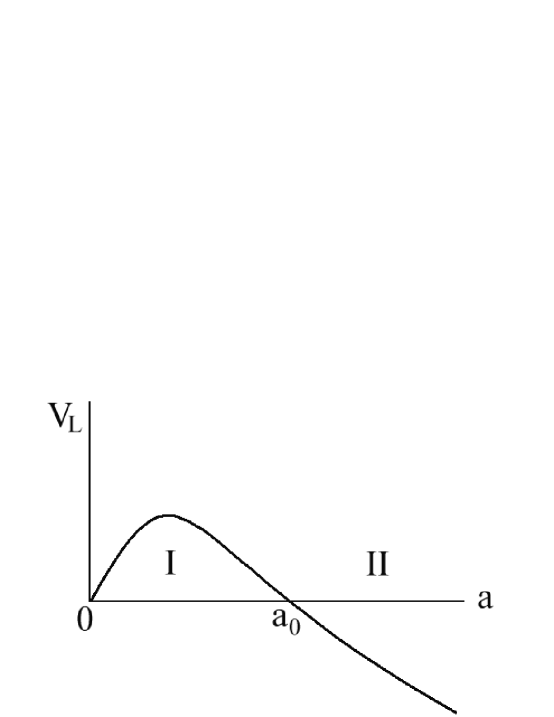
FIG. 1.: The effective potential $V_{L}$ vs. $a$ in the Lorentzian geometry. The gravitational field exhibits an exponential behavior in the Euclidean region I but oscillates in the Lorentzian region II.

- [1] S. W. Hawking and N. G. Turok, Phys. Lett. B 425, 25 (1998).
- [2] A. Linde, Phys. Rev. D 58, 083514 (1998); S. W. Hawking and N. Turok, ”Comment on ’Quantum Creation of an Open Universe’, by Andrei Linde”, gr-qc/9802062; Phys. Lett. B 432, 271 (1998).
- [3] J. B. Hartle and S. W. Hawking, Phys. Rev. D 28, 2960 (1983).
- [4] A. D. Linde, Lett. Nuovo Cimento 39, 401 (1984).
- [5] A. Vilenkin, Phys. Rev. D 30, 509 (1984); Phys. Rev. D 33, 3560 (1986).
- [6] A. Vilenkin, Phys. Rev. D 50, 2581 (1994); Phys. Rev. D 58, 067301 (1998); ”The quantum cosmology debate”, gr-qc/9812027.
- [7] N. D. Birrel and P. C. W. Davies, Quantum Fields in Curved Spacetime (Cambridge Univ. Press, Cambridge, United Kingdom, 1982).
- [8] For review and references see C. Kiefer, in Canonical Gravity: From Classical to Quantum, edited by J. Ehlers and H. Friedrich (Springer, Berlin, 1994).
- [9] R. Brout, Found. Phys. 17, 603, (1987); R. Brout, G. Horwitz, and D. Weil, Phys. Lett. B 192, 318 (1987); R. Brout, Z. Phys. B 68, 339 (1987); R. Brout and Ph. Spindel, Nucl. Phys. B348, 405 (1991).
- [10] R. Brout and G. Venturi, Phys. Rev. D 39, 2436 (1989); S. P. Kim and S.-W. Kim, Phys. Rev. D 49, R1679 (1994); C. Bertoni, and F. Finelli, and G. Venturi, Class. Quantum Grav. 13, 2375 (1996); R. Parentani, Phys. Rev. D 56, (1997).
- [11] S. P. Kim, Phys. Rev. D 52, 3382 (1995); Class. Quantum Grav. 13, 1377 (1996); Phys. Rev. D 55, 7511 (1997); Phys. Lett. A 236, 11 (1997).
- [12] S. P. Kim, J.-Y. Ji, H.-S. Shin, and K.-S. Soh, Phys. Rev. D 56, 3756 (1997); K. H. Cho, J. Y. Ji, S. P. Kim, C. H. Lee, and J. Y. Ryu, Phys. Rev. D 56, 4916 (1997).
- [13] S. P. Kim and S.-W. Kim, ”Quantum Tunneling Wave Functions of the Universe”, in preparation.