OUTP-99-09P, UPR-831T, PUPT-1837
hep-th/9902071
Boundary Inflation

Inflationary solutions are constructed in a specific five–dimensional model with boundaries motivated by heterotic M–theory. We concentrate on the case where the vacuum energy is provided by potentials on those boundaries. It is pointed out that the presence of such potentials necessarily excites bulk Kaluza–Klein modes. We distinguish a linear and a non–linear regime for those modes. In the linear regime, inflation can be discussed in an effective four–dimensional theory in the conventional way. We lift a four–dimensional inflating solution up to five dimensions where it represents an inflating domain wall pair. This shows explicitly the inhomogeneity in the fifth dimension. We also demonstrate the existence of inflating solutions with unconventional properties in the non–linear regime. Specifically, we find solutions with and without an horizon between the two boundaries. These solutions have certain problems associated with the stability of the additional dimension and the persistence of initial excitations of the Kaluza–Klein modes.

1 Introduction

Two important theoretical developments, the advent of M–theory and the discovery of branes have recently stimulated new ideas in early universe cosmology. There has been considerable activity on various cosmological aspects of M–theory over the past two years [1]–[24]. The cosmology of Hořava–Witten theory [25, 26, 27, 28], which describes M–theory on the orbifold $S^{1}/Z_{2}$, however, is much less studied so far [29, 30, 31, 32, 33]. This theory describes the strong coupling dual of the $E_{8}\times E_{8}$ heterotic string and is, therefore, of great importance for M–theory particle phenomenology. Clearly, this property makes it a very interesting starting point for cosmology as well.

Various aspects of branes might be important in early universe cosmology, such as their ability to smooth out singularities [5, 6, 11, 21, 22] and their thermodynamical properties [10, 12, 34, 35]. Most obviously, however, they play a role in the cosmology of particle physics models that have branes in their vacuum structure and, more specifically, that lead to low–energy theories arising from the worldvolumes of branes. Such models appear in the context of brane boxes [36, 37], type I string theory [38, 39, 40, 41] and M–theory on $S^{1}/Z_{2}$ [42, 43, 44, 45]. A characteristic feature of many of those models is the possibility of one or more compact dimensions being large compared to the fundamental length scale of the theory. Such a situation can be described by a Kaluza–Klein theory with gravity and possibly other fields in the bulk coupled to a four–dimensional “brane–like” object with the standard model fields on its worldvolume. A wide spectrum of scales has been proposed for such models. These range from fundamental scales around the GUT scale with the energy scale associated with the additional dimensions being an order of magnitude or so smaller, to models with a fundamental scale of order a TeV with macroscopic additional dimensions [46]. It is clearly interesting to explore the cosmology of these models and, recently, some work in this direction [47, 21, 31, 33, 48] has been done.

In this paper, we would like to study the important issue of how inflation relates to these new theoretical ideas. For recent related work on inflation see [20, 49, 50, 23, 24, 51]. Rather than presenting a general scenario, we will concentrate on a specific model which incorporates the M–theory as well as the brane aspects. This model can be interpreted as a part of the five–dimensional effective action of M–theory on $S^{1}/Z_{2}$ [42, 52, 43, 53] obtained by reducing the 11–dimensional theory on a Calabi–Yau three–fold. The five–dimensional space of this theory has the structure ${\cal M}_{5}=S^{1}/Z_{2}\times{\cal M}_{4}$ and contains two four–dimensional orbifold fixed planes (or boundaries) ${\cal M}_{4}^{(1)}$ and ${\cal M}_{4}^{(2)}$. It consists of gauged ${\cal N}=1$ supergravity plus vector– and hypermultiplets in the bulk coupled to ${\cal N}=1$ theories with gauge and chiral multiplets on the orbifold fixed planes. The vacuum solution of this theory [42] is a BPS double three–brane (domain wall) with the three–brane worldvolumes identified with the orbifold planes. Upon reduction to four dimensions on this vacuum solution, one arrives at an ${\cal N}=1$ supergravity theory which is a candidate for a realistic particle physics model from M–theory. The hidden and observable fields in this model arise from the “three–brane orbifold planes”. The theory, therefore, allows us to study cosmology in a potentially realistic particle physics environment and provides a concrete realization of the general idea of “getting the standard model from a brane”. Simple cosmological solutions of this theory have been found in ref. [31, 33]. In ref. [44, 45] non–perturbative vacua of heterotic M–theory containing five–branes have been constructed. In the five–dimensional effective theory, these five–branes appear as three–branes which, in addition to the two orbifold planes, are coupled to the bulk. It would clearly be interesting to study cosmological solutions of these more general theories with additional three–branes. In this paper, however, we restrict ourselves to the simple setting of two orbifold planes.

For the application to cosmology, we have (consistently) truncated this theory to a minimal field content suitable for inflationary models. Specifically, in the bulk we have kept gravity and a scalar field $\phi$ (the volume modulus of the internal Calabi–Yau space) with a potential $V$ of non–perturbative origin. In addition, on each orbifold plane we have also kept a scalar field $\phi_{i}$ with a potential $V_{4i}$. The theory is characterized by three scales, namely the fundamental scale $M_{5}$ of the five–dimensional theory, the separation $R$ of the orbifold planes and a scale $v$ that sets the height of certain explicit potentials for the bulk field $\phi$. These potentials are responsible for the existence of the domain wall solution.

Hence, we have a very simple setting with one additional dimension and one “candidate inflaton” with potential in each part of the space. In addition to the M–theory relation, we, clearly, also have a simple starting point to study inflation in the general context of models with large additional dimensions.

The goal of this paper is not to construct explicit inflationary models by choosing specific potentials for the scalar fields in the theory. Rather, we are interested in how the specific structure of the theory, that is, the coupling of the five–dimensional bulk to four–dimensional boundary theories, effects inflation. We distinguish two different types of inflation, which we call bulk (or moduli) and boundary (or matter field) inflation. For bulk inflation the vacuum energy is predominantly provided by the bulk potential $V$, whereas for boundary inflation the boundary potentials $V_{4i}$ dominate. In this paper, we concentrate on the second case of boundary inflation. This option is particularly interesting in that it directly relates to the presence of the characteristic boundary theories. Moreover, inflation from matter fields seems to be in better accord with current directions in four–dimensional inflationary model building [61] than modular inflation.

Let us summarize our main results. One of the main themes of this paper is that energy density on the orbifold planes provides source terms localized on the fixed points in the additional dimension and, hence, excites bulk fields. In particular, this applies to vacuum energy on these planes as needed for boundary inflation. Our first conclusion is that boundary inflation is necessarily inhomogeneous in the additional dimension, or, in other words, excites Kaluza–Klein modes. The magnitude of those excitations is controlled by the dimensionless parameter $\epsilon_{i}=V_{4i}R/M_{5}^{3}$. For $|\epsilon_{i}|\ll 1$ the excitations can be described by linearized gravity. This approximation breaks down if $|\epsilon_{i}|\gg 1$. One then has to use the full non–linear theory. Using the COBE normalization and the typical magnitude of heterotic M–theory scales, we argue that inflation in this theory may take place in both regimes. Interestingly, if the orbifold and Calabi–Yau scales during inflation are at their physical values [28], the theory becomes linear for $V_{4i}^{1/4}\ll 6\cdot 10^{16}$ GeV, right below the COBE scale.

The proportionality of $\epsilon_{i}$ to the size $R$ of the additional dimension can be understood from the linear behaviour of the one–dimensional Green’s function. For more than one additional dimension, the Green’s function is logarithmic or follows an inverse power law. As a consequence, in those cases, the theory is always in the linear regime. The case of heterotic M–theory with one large dimension is, therefore, the only one where inflation may take place in the non–linear regime.

In the linear regime, we can compute a sensible four–dimensional effective theory by integrating out the Kaluza–Klein modes induced by the boundary sources. We show explicitly how this leads to corrections in the four–dimensional theory. Our basic statement is that, in the linear regime, inflation can essentially be treated in the effective four–dimensional ${\cal N}=1$ supergravity theory. Nevertheless, to get a physical picture, we find it useful to lift a generic four–dimensional inflating solution up to a five–dimensional one. This five–dimensional solution represents a pair of inflating domain wall three–branes and it has inhomogeneities in the additional dimension caused by the boundary potentials. On the other hand, initial inhomogeneities not induced by boundary sources are damped away in the linear regime due to the inflationary expansion and should not play any role.

The situation is quite different in the non–linear regime, $\epsilon_{i}\gg 1$, where one has to solve the full five–dimensional theory. To do so, we assume that the bulk scalar field $\phi$ has been stabilized by its potential and the boundary potentials allow for slow roll behaviour of the boundary scalars. Under these assumptions we find, in a first attempt, a simple solution by separation of variables that exhibits inflation. This solution represents the heterotic M–theory version of an old four–dimensional domain wall solution [62, 63], recently advocated [50] in a somewhat different approach to brane inflation. Both boundaries expand in a de Sitter–like manner with the Hubble parameters $H_{i}$ related to the potentials in an unconventional way, $H_{i}\sim|V_{4i}|M_{5}^{-3}$. The physical size $R_{\rm phys}$ of the additional dimension is constant in time and fixed in terms of the boundary potentials. For $H_{1}$ and $H_{2}$ of the same order, $H_{1}\sim H_{2}\sim H$, one has $R_{\rm phys}\sim 1/H$. The Hubble parameter, therefore, equals the orbifold energy scale during inflation. We find solutions with and without an horizon at some point on the orbifold. The solutions without horizon require potentials with opposite sign satisfying $V_{41}+V_{42}<0$. Signals travel from one boundary to the other in a finite time and every signal emitted somewhere in the bulk will eventually reach one of the boundaries. For the solutions with horizon one needs both potentials to be positive, $V_{4i}>0$. In this case, the two boundaries are causally decoupled. A signal emitted on one boundary will never reach the other one.

In a second approach, we then find the general solution of the model without assuming separation of variables. This is done exploiting the similarity of our equations to those of two–dimensional dilaton gravity [70]. We recover the previous inflating solution as a special case if a certain continuous parameter in the general solution is set to zero. For all other values of this parameter, however, the solution is non–inflating and has a collapsing orbifold. This indicates an instability of the solution which might be cured by stabilizing the modulus of the additional dimension. The construction of a viable inflationary background in the non–linear regime is, therefore, tied to the question on how precisely such a stabilization is realized. We discuss various options and their consequences in our context. Another problem with the inflating solution which is made visible by its generalization is the appearance of an arbitrary periodic function in the solution. This function encodes the initial inhomogeneities in the additional dimension. Unlike in the linear case, here these inhomogeneities are not damped away. This seems to be in contradiction with the inflationary paradigm that all initial information should be wiped out. On the other hand, if sufficiently small, these inhomogeneities may lead to interesting predictions. Given those problems, we point out that conventional inflation in the linear regime remains a perfectly viable option for heterotic M–theory. For models with more than one large dimension it is the only possibility.

Based on the results of this paper, we would like to propose three scenarios for inflation in heterotic M–theory.

• The orbifold and the Calabi–Yau scales during inflation are at the specific values that at low-energy lead to coupling unification. In this case, the theory becomes linear for boundary potentials satisfying $V_{4i}^{1/4}\ll V_{\rm lin}^{1/4}\simeq 6\cdot 10^{16}$ GeV. At the unification point the Calabi–Yau scale and the fundamental 11–dimensional Planck scale are also of the order $10^{16}$ GeV. This theory undergoes a transition from a pure M–theory regime at energies above $10^{16}$ GeV (where no description in terms of 11–dimensional supergravity applies) directly to the linear regime. Inflation can then take place in the conventional way, presented in this paper. In this scenario, the energy density at the beginning of inflation is directly linked to the fundamental scales of the theory and is, in this sense, explained. It fits the COBE normalization $V_{4}^{1/4}\simeq\varepsilon^{1/4}\,6.7\cdot 10^{16}$ GeV if the slow–roll parameter $\varepsilon$ is not too small, or, in other words, if the inflaton potential is not too flat.

An alternative possibility is that the orbifold and Calabi–Yau scales are not be at the coupling unification values during inflation. Rather, they are such that the linear regime starts significantly below $10^{16}$ GeV, $V_{\rm lin}^{1/4}\ll 10^{16}$ GeV. In this case, there are two options.

• Inflation takes place in the non–linear regime and is based on the corresponding solutions given in this paper. This option is somewhat speculative as it depends on the successful stabilization of the orbifold modulus. It would have very unconventional properties. These include a linear relation between the Hubble parameter and the potential and inhomogeneities in the orbifold direction. Since space–time in this context is genuinely five–dimensional, analyzing density fluctuations requires some care and the standard equations may not apply.

• Non–linear inflation does not take place. This might happen for a number of reasons. For example, the potentials might not have the required properties, the initial conditions may not be appropriate or, simply, non–linear inflation might not work at all. Inflation could then start when the energy density drops below $V_{\rm lin}$ and the linear regime is reached. This could be consistent with the COBE normalization for a very small slow–roll parameter $\varepsilon$, that is, a very flat inflaton potential.

2 The action

In this section, we would like to present the five–dimensional action that we are going to use in this paper along with its most important properties. This includes a discussion of its origin and interpretation, its “vacuum” solution and the related four–dimensional effective low–energy theory that is obtained as a reduction on this vacuum solution. Making contact with the four–dimensional theory is particularly useful, in our context, whenever the relation to “conventional” four–dimensional inflation is analyzed.

Our starting point is the five–dimensional action 

$$S_{5} = -\frac{1}{2\kappa_{5}^{2}}\left\{\int_{{\cal M}_{5}}\sqrt{-g}\left[R+\frac{1}{2}\partial_{\alpha}\phi\partial^{\alpha}\phi+U(\phi)\right]\right.$$ (2.1)

$$\qquad\qquad\left.+\sum_{i=1}^{2}\int_{{\cal M}_{4}^{(i)}}\sqrt{-g}\left[\frac{1}{2}\partial_{\mu}\phi_{i}\partial^{\mu}\phi_{i}+U_{i}(\phi_{i},\phi)\right]\right\}$$

where the potentials are given by

$$U(\phi) = \frac{1}{3}v^{2}e^{-2\phi}+V(\phi)$$ (2.2)

$$U_{i}(\phi_{i},\phi) = \mp 2\sqrt{2}ve^{-\phi}+V_{i}(\phi_{i},\phi)\;.$$ (2.3)

Here $\kappa_{5}$ is the five–dimensional Newton constant. Coordinates $x^{\alpha}$ with indices $\alpha,\beta,\gamma,\dots=0,\dots,3,5$ are used for the five–dimensional space ${\cal M}_{5}$. We consider a space–time with structure ${\cal M}_{5}=S^{1}/Z_{2}\times{\cal M}_{4}$ where $S^{1}/Z_{2}$ is an orbifold and ${\cal M}_{4}$ a smooth four–manifold. The coordinates $x^{\mu}$ on ${\cal M}_{4}$ are labelled by indices $\mu,\nu,\rho,\dots=0,\dots,3$ while the remaining coordinate $y\equiv x^{5}$ parameterizes the orbifold. It is chosen in the range $y\in[-R,R]$ with the endpoints identified, where $R=\pi\rho$ and $\rho$ is the radius of the orbicircle. The $Z_{2}$ symmetry acts as $y\rightarrow-y$ and leaves two four–dimensional planes, characterized by $y_{1}=0$ and $y_{2}=R$, fixed. These planes, separated by a distance $R$, are denoted by ${\cal M}_{4}^{(i)}$, where $i=1,2$. The action (2.1) describes five–dimensional gravity plus a scalar field $\phi$ with potential $U$ in the bulk coupled to four–dimensional theories on the orbifold fixed planes each carrying a scalar field $\phi_{i}$ with potential $U_{i}$. The bulk fields have to be truncated in accordance with the $Z_{2}$ symmetry. Specifically, one should require

$$\phi(-y) = \phi(y)$$

$$g_{\mu\nu}(-y) = g_{\mu\nu}(y)$$

$$g_{\mu 5}(-y) = -g_{\mu 5}(y)$$ (2.4)

$$g_{55}(-y) = g_{55}(y)\;.$$

Hence, $\phi$, $g_{\mu\nu}$, $g_{55}$ are even under the $Z_{2}$ symmetry while $g_{\mu 5}$ is odd. Also note that the $y$–derivative of an even field is odd and vice versa. Whereas even fields are continuous across the orbifold planes, odd field jump from a certain value on one side to its negative on the other side. An alternative and equivalent way to think about the five–dimensional space, in contrast to the orbifold picture which we have used so far, is the boundary picture. In this picture, the coordinate $y$ is restricted to one half of the circle, $y\in I=[0,R]$ and five–dimensional space–time is written as ${\cal M}_{5}=I\times{\cal M}_{4}$. The orbifold fixed planes then turn into the boundaries of this five–dimensional space. We will sometimes find it more convenient to work in this boundary picture.

The potentials (2.2) and (2.3) have been split into explicit, exponential potentials for $\phi$ with a height set by the constant $v$ and potentials $V$ and $V_{i}$ which, at this point, are arbitrary. The $-$ sign in (2.3) refers to the plane $i=1$, the $+$ sign to the plane $i=2$. The reason for writing the potentials in this form will be explained shortly. It is useful to collect the mass dimensions of the various objects that we have introduced. In five dimensions, the Newton constant $\kappa_{5}^{-2}$ has dimension three and we write

$$\kappa_{5}^{-2}=M_{5}^{3}\;.$$ (2.5)

Here $M_{5}$ is the “fundamental” scale of the five–dimensional theory. In order to make subsequent equations simpler, we have pulled the Newton constant in front of the complete action. Hence, the bulk potentials $U$, $V$ have dimension two whereas the boundary potentials $U_{i}$, $V_{i}$ and the constant $v$ have dimension one.

Let us now discuss the interpretation of the action (2.1)–(2.3) in terms of M–theory. More specifically, we will consider Hořava–Witten theory; that is, 11–dimensional supergravity on the space $S^{1}/Z_{2}\times{\cal M}_{10}$ where ${\cal M}_{10}$ is a smooth ten–dimensional manifold. The two 10–dimensional orbifold fixed planes of this theory carry additional degrees of freedom that couple to the bulk supergravity, namely two $E_{8}$ gauge multiplets, one on each plane. Now consider reducing this theory on a Calabi–Yau three–fold assuming that the radius of the Calabi–Yau space is smaller than the orbifold radius. For the present values of these radii, such a relation is suggested by coupling constant unification [28]. We then arrive at a sensible five–dimensional theory on the space–time ${\cal M}_{5}=S^{1}/Z_{2}\times{\cal M}_{4}$, where the two four–dimensional fixed planes of the orbifold result from the original 10–dimensional planes. For the standard embedding of the spin connection into one of the $E_{8}$ gauge groups, this effective action has been computed in ref. [42, 52, 43]. The generalization to non–standard embedding has been described in ref. [54]. It turns out that the bulk theory is a five–dimensional ${\cal N}=1$ gauged supergravity coupled to vector– and hypermultiplets. This bulk theory is coupled to two four–dimensional ${\cal N}=1$ theories that reside on the now four–dimensional orbifold planes. More specifically, these boundary theories contain gauge multiplets as well as chiral (gauge matter) multiplets. Upon appropriate reduction on the orbifold to four dimensions (in a way to be specified below), one obtains a candidate for a “realistic” ${\cal N}=1$ supergravity theory with the observable sector coming from one plane and the hidden sector from the other.

The action (2.1) is a “universal” version of this five–dimensional effective theory truncated to the field content that seems essential to discuss cosmology. Let us try to make this statement more precise by explaining the meaning of the various objects in (2.1)–(2.3) in terms of the underlying 11–dimensional theory. In terms of the 11–dimensional Newton constant $\kappa$ and the Calabi–Yau volume $v_{\rm CY}$ the five–dimensional Newton constant is given by

$$\kappa_{5}^{2}=\frac{\kappa^{2}}{v_{\rm CY}}\;.$$ (2.6)

The bulk field $\phi$ is simply the modulus associated with the Calabi–Yau volume such that the “physical” volume is given by $e^{\phi}v_{\rm CY}$. Clearly, the Calabi–Yau space has, in general, many more moduli associated with its shape and complex structure. For simplicity, we have kept the volume modulus only, since it is the geometrical modulus common to all Calabi–Yau spaces. It is in this sense that we are referring to the action as universal. Also, for simplicity, we have dropped a number of other bulk fields such as the axions associated with $\phi$ and the vector fields in the vector multiplets. All these fields can be consistently set to zero in the full equations of motion. Therefore, our solutions will be solutions of the complete action of heterotic M–theory as well. We have, however, kept a feature of the action that arises from the gauging of the bulk supergravity and is essential to discuss cosmology; namely, the explicit bulk potential for $\phi$ in eq. (2.2). The constant $v$ in this potential is given by

$$v=-\frac{\pi}{\sqrt{2}}\left(\frac{\kappa}{4\pi}\right)^{2/3}\frac{n}{v_{\rm CY}^{2/3}}$$ (2.7)

where $n$ is an instanton number related to the tangent space and gauge instantons in the internal Calabi–Yau space. We have added another potential $V(\phi)$ in the bulk which one expects to arise from non–perturbative effects like internally wrapped membranes. The explicit computation of this potential for M–theory is not very well understood at present (see however [55, 56]). It is, however, clear that such a potential is eventually needed to stabilize the moduli. Given the lack of theoretical knowledge, we will not assume any specific origin for $V$ but, rather, try to specify what properties it should be required to have from a cosmological viewpoint.

Let us now move on to the four–dimensional theories on the orbifold planes and their M–theory origin. As already mentioned, these planes arise directly from the 10–dimensional planes of Hořava–Witten theory upon reduction on the Calabi–Yau space. On each of these planes, we have introduced a scalar field $\phi_{i}$ with potential $U_{i}$ that represents the scalar partners of the matter fields. In fact, for non–standard embedding such matter fields generally arise on both planes. Of course, restricting to one scalar field on each plane is a tremendous simplification from the particle physics point of view. Cosmologically, however, it seems reasonable to choose such a model with one “candidate inflaton” on each orbifold plane, especially in a first study of inflation in such models. Although the potentials $V_{i}$ in eq. (2.3) are known in principle for a given Calabi–Yau compactification, here we will not attempt to be more specific about their form. Instead of going into such detailed questions of model building, we will assume that they have the cosmologically desired properties. There is another, explicit part of the boundary potential in eq. (2.3) which depends on the projection of the bulk field $\phi$ onto the orbifold planes. These potentials originate directly from Hořava–Witten theory and are related to the explicit bulk potential for $\phi$. Note that, in particular, the height is set by the same constant $v$, defined in eq. (2.7). As we will see, they support a three–brane domain wall solution of the five–dimensional theory. In the following, we, therefore, refer to them as domain wall potentials. Of course, there will be gauge multiplets on the orbifold planes as well which we have not written in (2.1). They could play a role in cosmology via gaugino condensation. However, we will not consider this explicitly in the present paper. To summarize, the action (2.1)–(2.3) can be viewed as part of the five–dimensional effective theory of heterotic M–theory and it contains the basic cosmologically relevant ingredients of this theory.

The M–theory context is not obligatory here. Instead, the action (2.1) could be viewed in the general context of theories with large additional dimensions where the standard model arises from a brane worldvolume. In fact, in this context, our action is about the simplest appropriate to study inflationary cosmology. We have one “large” dimension (the orbifold) and two four–dimensional brane–like theories corresponding to an observable and a hidden sector. In addition to bulk gravity, we have a bulk scalar field with potential and a scalar field with potential on each plane; in other words, a minimal setting for inflation. The explicit potentials in (2.2), (2.3) that originate from M–theory can always be switched off by setting $v=0$, if desired. Our results are, therefore, not limited by their presence. What does limit our results is the presence of only one additional dimension, something that is appropriate for heterotic M–theory but not necessarily otherwise. We will comment on the modification of our results in the case of two or more large dimensions as we proceed.

For later reference, let us collect the equations of motion derived from the action (2.1). We have the Einstein equation

$$R_{\alpha\beta}-\frac{1}{2}g_{\alpha\beta}R=T_{\alpha\beta}+\sum_{i=1}^{2}T_{\alpha\beta}^{(i)}\delta(y-y_{i})$$ (2.8)

with the bulk and boundary energy momentum tensors

$$T_{\alpha\beta} = -\frac{1}{2}\left(\partial_{\alpha}\phi\partial_{\beta}\phi-\frac{1}{2}g_{\alpha\beta}(\partial\phi)^{2}\right)+\frac{1}{2}g_{\alpha\beta}U$$ (2.9)

$$T_{\mu\nu}^{(i)} = -\frac{1}{2}g_{55}^{-1/2}\left(\partial_{\mu}\phi_{i}\partial_{\nu}\phi_{i}-\frac{1}{2}g_{\mu\nu}(\partial\phi_{i})^{2}-g_{\mu\nu}U_{i}\right)$$ (2.10)

$$T_{\mu 5}^{(i)} = 0\;,\qquad T_{55}^{(i)}=0\;.$$ (2.11)

For the scalar fields we find

$$\Box_{5}\phi-\partial_{\phi}U-g_{55}^{-1/2}\sum_{i=1}^{2}\partial_{\phi}U_{i}\delta(y-y_{i}) = 0$$ (2.12)

$$\Box_{4}\phi_{i}-\partial_{\phi_{i}}V_{i} = 0$$ (2.13)

where $\Box_{5}$ and $\Box_{4}$ are the Laplacians associated with the five–dimensional metric $g_{\alpha\beta}$ and its four–dimensional part $g_{\mu\nu}$ projected onto one of the orbifold planes.

Which types of solutions to these equations are we interested in? For a cosmological solution, one would like to have a three–dimensional maximally symmetric subspace which, for simplicity, we take to be flat. Studying open and closed universes would be clearly interesting as well. Later, we will distinguish between a linear and a non–linear case. While the generalization to include spatial curvature is straightforward in the linear case, the non–linear case is significantly more complicated. Still, we do not expect our main conclusions to depend on the choice of spatial curvature. Clearly, the maximally symmetric subspace cannot contain the orbifold. Hence, the solutions are independent of ${\bf x}=(x^{1},x^{2},x^{3})$. They can, however, depend on the time $\tau=x^{0}$ as well as on the orbifold coordinate $y$. As we will see in a moment, the presence of fields and potentials on the boundaries in fact forces us to consider orbifold dependence. Therefore, we start with the ansatz

$$ds_{5}^{2} = -e^{2\nu}d\tau^{2}+e^{2\alpha}d{\bf x}^{2}+e^{2\beta}dy^{2}$$ (2.14)

$$\nu = \nu(\tau,y)$$ (2.15)

$$\alpha = \alpha(\tau,y)$$ (2.16)

$$\beta = \beta(\tau,y)$$ (2.17)

$$\phi = \phi(\tau,y)$$ (2.18)

$$\phi_{i} = \phi_{i}(\tau)\;.$$ (2.19)

Here $\alpha$ is the scale factor of the three–dimensional universe and $\beta$ is an additional scale factor that measures the orbifold size. In some cases, we will choose the conformal gauge $\nu=\beta$ in the above metric. Note that we can choose this gauge in the $(\tau,y)$ subspace in such a way that the boundaries are mapped to hypersurfaces $y=$ const. Usually, then, we can shift the boundaries back to $y=0,R$ so that our conventions for the coordinate system remain intact. A special case occurs if a boundary has been “mapped to infinity” due to a singularity in the reparameterization. To be able to deal with this case, we keep $\nu$ arbitrary in the subsequent formulae.

The equations of motion for the above ansatz are given by

$$3e^{-2\nu}(\dot{\alpha}^{2}+\dot{\alpha}\dot{\beta})-3e^{-2\beta}(\alpha^{\prime\prime}-\alpha^{\prime}\beta^{\prime}+2{\alpha^{\prime}}^{2})=\\ \frac{1}{4}e^{-2\nu}\dot{\phi}^{2}+\frac{1}{4}e^{-2\beta}{\phi^{\prime}}^{2}+\frac{1}{2}U+\frac{1}{2}e^{-\beta}\sum_{i=1}^{2}\left[\frac{1}{2}e^{-2\nu}\dot{\phi}_{i}^{2}+U_{i}\right]\delta(y-y_{i})$$ (2.20)

$$e^{-2\nu}(2\ddot{\alpha}+\ddot{\beta}+(3\dot{\alpha}+2\dot{\beta}-2\dot{\nu})\dot{\alpha}+(\dot{\beta}-\dot{\nu})\dot{\beta})-\\ e^{-2\beta}(2\alpha^{\prime\prime}+\nu^{\prime\prime}+(3\alpha^{\prime}-2\beta^{\prime}+2\nu^{\prime})\alpha^{\prime}+(\nu^{\prime}-\beta^{\prime})\nu^{\prime})\\ =-\frac{1}{4}e^{-2\nu}\dot{\phi}^{2}+\frac{1}{4}e^{-2\beta}{\phi^{\prime}}^{2}+\frac{1}{2}U-\frac{1}{2}e^{-\beta}\sum_{i=1}^{2}\left[\frac{1}{2}e^{-2\nu}\dot{\phi}_{i}^{2}-U_{i}\right]\delta(y-y_{i})$$ (2.21)

$$3e^{-2\nu}(\ddot{\alpha}-\dot{\nu}\dot{\alpha}+2\dot{\alpha}^{2})-3e^{-2\beta}({\alpha^{\prime}}^{2}+\nu^{\prime}\alpha^{\prime}) = -\frac{1}{4}e^{-2\nu}\dot{\phi}^{2}-\frac{1}{4}e^{-2\beta}{\phi^{\prime}}^{2}+\frac{1}{2}U$$ (2.22)

$$3(\dot{\alpha}^{\prime}+\dot{\alpha}\alpha^{\prime}-\dot{\alpha}\nu^{\prime}-\dot{\beta}\alpha^{\prime}) = -\frac{1}{2}\dot{\phi}\phi^{\prime}$$ (2.23)

$$e^{-2\nu}(\ddot{\phi}+(3\dot{\alpha}+\dot{\beta}-\dot{\nu})\dot{\phi})-e^{-2\beta}(\phi^{\prime\prime}+(3\alpha^{\prime}-\beta^{\prime}+\nu^{\prime})\phi^{\prime}) = -\partial_{\phi}U-e^{-\beta}\sum_{i=1}^{2}\partial_{\phi}U_{i}\delta(y-y_{i})$$ (2.24)

$$\ddot{\phi}_{i}+(3\dot{\alpha}-\dot{\nu})\dot{\phi}_{i}+e^{2\nu}\partial_{\phi_{i}}V_{i} = 0$$ (2.25)

where the dot and the prime denote the derivatives with respect to $\tau$ and $y$. Alternatively, one can formulate these equations in the boundary picture. Then all $\delta$ function terms in the above equations have to be dropped and are replaced by the following boundary conditions

$$e^{-\beta}\alpha^{\prime}\left.\right|_{y=y_{i}} = \mp\frac{1}{12}\left[\frac{1}{2}e^{-2\nu}\dot{\phi}_{i}^{2}+U_{i}\right]_{y=y_{i}}$$ (2.26)

$$e^{-\beta}\nu^{\prime}\left.\right|_{y=y_{i}} = \mp\frac{1}{12}\left[-\frac{5}{2}e^{-2\nu}\dot{\phi}_{i}^{2}+U_{i}\right]_{y=y_{i}}$$ (2.27)

$$e^{-\beta}\phi^{\prime}\left.\right|_{y=y_{i}} = \pm\frac{1}{2}\left[\partial_{\phi}U_{i}\right]_{y=y_{i}}\;.$$ (2.28)

Here the upper (lower) sign applies to the first boundary at $y=y_{1}$ (the second boundary at $y=y_{2}$). The $\delta$–function terms, or equivalently the right hand sides of the boundary conditions, are non–vanishing if there is any kinetic or potential energy on the boundaries. Hence, in this most interesting case, the solution is necessarily inhomogeneous in the orbifold coordinate $y$.

For the application to cosmology, one is also interested in the four–dimensional effective action of (2.1) that is, roughly speaking, valid when all energy scales are smaller than the orbifold scale $1/R$. Normally, this action could be derived by a simple truncation where all the bulk fields are taken to be independent of the orbifold coordinate. While, in our case, this gives the correct answer to lowest order, it neglects higher order corrections that can be relevant. These corrections appear because, strictly, we are not allowed to take the bulk fields independent of the orbifold coordinate, thereby neglecting all contributions from Kaluza–Klein modes. Instead, as we have just seen, every non–vanishing term in the boundary actions produces an orbifold dependence that needs to be integrated out and, typically, leads to corrections to the effective action. Let us explain how this works in our case, taking into account corrections up to the first non–trivial (linear) order. For a more detailed account see [57]. First, we split the bulk fields as

$$g_{\alpha\beta} = \bar{g}_{\alpha\beta}+\tilde{g}_{\alpha\beta}$$ (2.29)

$$\phi = \bar{\phi}+\tilde{\phi}$$ (2.30)

into their orbifold average plus an orbifold–dependent variation. Specifically, we have defined

$$\bar{g}_{\alpha\beta}=<g_{\alpha\beta}>_{5}\;,\qquad\bar{\phi}=<\phi>_{5}$$ (2.31)

where $<.>_{5}$ denotes the average in the orbifold direction. Hence, the average of the variations vanishes; that is,

$$<\tilde{g}_{\alpha\beta}>_{5}=0\;,\qquad<\tilde{\phi}>_{5}=0\;.$$ (2.32)

The averaged fields are in one to one correspondence with the low energy moduli fields. Aside from the modulus $\bar{\phi}$, we have the orbifold modulus $\bar{\beta}$ and the four–dimensional Einstein–frame metric $g_{4\mu\nu}$. The latter two quantities are related to the averaged metric by

$$e^{2\bar{\beta}} = \bar{g}_{55}$$ (2.33)

$$g_{4\mu\nu} = e^{\bar{\beta}}\bar{g}_{\mu\nu}\;.$$ (2.34)

Note that we have no graviphoton zero mode since $g_{\mu 5}$ is odd under $Z_{2}$ and, hence, $\bar{g}_{\mu 5}=0$. After expanding to linear order in the variations, the equations of motion can be decomposed into an averaged part and a part for the variations. The latter equations have the following solutions in the boundary picture 

$$\tilde{g}_{\alpha\beta} = e^{2\bar{\beta}}R\left[P_{1}(z)\bar{S}_{\alpha\beta}^{(1)}+P_{2}(z)\bar{S}_{\alpha\beta}^{(2)}\right]$$ (2.35)

$$\tilde{\phi} = \frac{1}{2}e^{\bar{\beta}}R\left[P_{1}(z)\overline{\partial_{\phi}U_{1}}+P_{2}(z)\overline{\partial_{\phi}U_{2}}\right]$$ (2.36)

where

$$S_{\alpha\beta}^{(i)}=T_{\alpha\beta}^{(i)}-\frac{1}{3}g_{\alpha\beta}g^{\gamma\delta}T_{\gamma\delta}^{(i)}$$ (2.37)

is the modified boundary stress energy. The bar indicates that the corresponding expressions are understood with the bulk fields replaced by their zero modes. Furthermore, we have defined the polynomials 

$$P_{1}(z)=-\frac{1}{2}z^{2}+z-\frac{1}{3}\;,\qquad P_{2}(z)=-\frac{1}{2}z^{2}+\frac{1}{6}$$ (2.38)

which depend on the normalized orbifold coordinate

$$z=\frac{y}{R}\in[0,1]\;.$$ (2.39)

This solution shows that each energy source on the boundary leads to a certain, generally quadratic, $z$–dependent variation of the bulk fields across the orbifold. This corresponds to coherent excitations of the Kaluzu–Klein modes in the orbifold direction. Let us consider an explicit example. We would like to determine the $z$–dependence of the bulk fields that arises from the explicit boundary potentials in (2.3) proportional to $v$. Inserting the corresponding part of the boundary stress energy into eq. (2.35) and (2.36) we find

$$ds_{5}^{2} = (\bar{g}_{\alpha\beta}+\tilde{g}_{\alpha\beta})dx^{\alpha}dx^{\beta}=\left(1+\frac{1}{3}\tilde{\phi}\right)e^{-\bar{\beta}}g_{4\mu\nu}dx^{\mu}dx^{\nu}+\left(1+\frac{4}{3}\tilde{\phi}\right)e^{2\bar{\beta}}dy^{2}$$ (2.40)

$$\phi = \bar{\phi}+\tilde{\phi}$$ (2.41)

$$\tilde{\phi} = -2e^{\bar{\beta}-\bar{\phi}}\epsilon_{\rm DW}\left(z-\frac{1}{2}\right)$$ (2.42)

where

$$\epsilon_{\rm DW}=-\frac{vR}{\sqrt{2}}\;.$$ (2.43)

Note that the explicit potentials have the same height but opposite sign on the two boundaries. Therefore, the $z$–dependent part of the solution is proportional to the difference $(P_{1}-P_{2})(z)$ of the polynomials (2.38) and, hence, is linear in $z$. This is to be contrasted to the general case of unrelated boundary potentials which leads to a quadratic variation. For constant moduli $g_{4\mu\nu}$, $\bar{\beta}$ and $\bar{\phi}$, eq. (2.40)–(2.43) represent the linearized version of an exact BPS domain wall (three–brane) solution of heterotic M–theory  in five dimensions that was found in ref. [42]. More precisely, the solution represents a pair of domain walls stretched across the orbifold planes and it can be viewed as the “vacuum” solution of the theory. At the same time, it is the five–dimensional version of Witten’s 11–dimensional linearized background [28]. In this way, the four–dimensional orbifold planes are identified with three–brane worldvolumes which carry the observable (and hidden) low energy fields as their zero modes. In this sense, our picture offers a concrete realization of the general idea that the world arises from the worldvolume of a brane. Observe that the size of the correction (2.40) is set by the dimensionless quantity $\epsilon_{\rm DW}$ in eq. (2.43), which is just the product of the boundary potential (measured in units of $\kappa_{5}^{-2}=M_{5}^{3}$) times the size of the orbifold dimension. Therefore, the linearized approximation that led us to the solution (2.35), (2.36) is only sensible as long as $|\epsilon_{\rm DW}|\ll 1$. We will discuss this in more detail in the next section.

By inserting the solution (2.29)–(2.36) into the action (2.1) and promoting the moduli $g_{4\mu\nu}$, $\bar{\beta}$ and $\bar{\phi}$ to four–dimensional fields, we can now compute the first order corrected action of the zero modes. We introduce the fields

$$S=e^{\bar{\phi}}\;,\qquad T=e^{\bar{\beta}}$$ (2.44)

which are just the real parts of the ordinary $S$– and $T$–moduli . Note that $S$ measures the volume of the internal Calabi–Yau space in units of $v_{\rm CY}$ whereas $T$ measures the size of the orbifold in units of $R$. We also introduce the four–dimensional Newton constant

$$G_{N}=\frac{\kappa_{5}^{2}}{16\pi R}=\frac{1}{16\pi RM_{5}^{3}}$$ (2.45)

and the rescaled boundary fields

$$C_{i}=\sqrt{\frac{M_{5}^{3}}{3}}\phi_{i}\;.$$ (2.46)

Then the four–dimensional effective action is given by

$$S_{4} = -\frac{1}{16\pi G_{N}}\int_{M_{4}}\sqrt{-g_{4}}\left[R_{4}+\frac{3}{2}T^{-2}\partial_{\mu}T\partial^{\mu}T+\frac{1}{2}S^{-2}\partial_{\mu}S\partial^{\mu}S\right]$$ (2.47)

$$-\int_{M_{4}}\sqrt{-g_{4}}\left[\frac{1}{2}\sum_{i=1}^{2}K_{i}\partial_{\mu}C_{i}\partial^{\mu}C_{i}+V_{4}\right]$$

with the “Kähler metrics”

$$K_{i}=\frac{3}{2T}\pm\frac{\epsilon_{\rm DW}}{2S}$$ (2.48)

and the four–dimensional potential

$$V_{4}=\frac{1}{2T^{2}}\sum_{i=1}^{2}V_{4i}+\frac{\epsilon_{\rm DW}}{2ST}\sum_{i=1}^{2}\left(\pm\frac{2}{3}V_{4i}\pm\partial_{\bar{\phi}}V_{4i}\right)+\frac{1}{T}RM_{5}^{3}V$$ (2.49)

where the boundary potentials $V_{4i}$ normalized to four mass dimensions are defined by

$$V_{4i}=M_{5}^{3}V_{i}\;.$$ (2.50)

Note that the Kähler metrics and the potential have corrections linear in $\epsilon_{\rm DW}$ that originate from the domain wall. Had we performed a simple truncation of the five–dimensional theory by taking the bulk fields independent of the orbifold we would have missed these corrections. What happened to the explicit potentials proportional to $v$ in the five–dimensional action, eq. (2.2) and (2.3)? These potentials were actually responsible for the existence of the domain wall solution in the first place. Performing a reduction on this solution, they are canceled so that there is no remnant potential for the $S$ and $T$ moduli in four dimensions. Given the form of our five–dimensional action (2.1)–(2.3), the bulk potential $V$ only depends on $S$ but not on $T$. The four–dimensional effective potential (2.49) shows that, in this case, the modulus $T$ cannot be stabilized. For the solutions based on the four–dimensional effective action we, therefore, have to slightly generalize our setup and assume that $V$ is a function of the orbifold modulus $T$ as well.

An alternative way to deal with the orbifold dependence of bulk fields in a reduction to four dimensions is to keep all the Kaluza–Klein modes instead of integrating them out. Recently, this has systematically been carried out in ref. [59]. In such a four–dimensional action, the zero mode part does not have the above corrections. Instead, there exist terms in the action which couple Kaluza–Klein modes linearly to zero mode fields. Hence the Kaluza–Klein modes cannot be set to zero consistently. In fact, solving for these Kaluza–Klein modes would lead to the Fourier decomposition of our orbifold–dependent corrections (2.35), (2.36).

Besides being useful to calculate the four–dimensional action, the method described above can also be used to find approximate solutions of the five–dimensional theory. This is actually the main reason why we have presented it here in some detail. Concretely, suppose one has found a solution of the four–dimensional theory with action (2.47). Then, by inserting this solution into eq. (2.29)–(2.36), we can simply “lift it up” to obtain a solution of the five–dimensional theory. Of course, for this solution to be sensible, the linearized approximation that led us to eq. (2.35), (2.36) should be valid. The condition for that to be true will be discussed in the next section in some detail.

3 Types of inflation and scales

Which type of inflation for the action (2.1) do we want to consider? First of all, in this paper we are interested in “conventional” potential–driven inflation rather than in a pre–big–bang–type scenario [60]. Some solutions of five–dimensional heterotic M–theory that might provide a basis for a pre–big–bang scenario have been found in ref. [31, 32, 33]. Given that we want to focus on potential energy, there are two obvious options.

• bulk potential energy: The potential energy is provided by the bulk potential $V$ and the field $\phi$ is the inflaton. This can also be called “modular inflation”.

• boundary potential energy: The potential energy is due to the boundary potentials $V_{i}$ (one of them or both) and the fields $\phi_{i}$ are the inflatons. This can be called “matter field inflation”.

Clearly, in general, one could also have a mixture of both types. In this paper, we concentrate on the second option of boundary potential energy, which appears to be more interesting for a number of reasons. Most importantly, the presence of the boundaries is the truely new ingredient in the action (2.1). Inflation from the boundary also seems to be in accord with the current mainstream in four–dimensional inflationary model–building [61]. On the other hand, modular inflation faces a number of problems associated with the steepness of typical non–perturbative moduli potentials [64, 65]. From the viewpoint of the recently proposed models [46] with a very low “fundamental” scale $M_{5}\sim$ TeV, bulk inflation might not be desirable because reheating from a bulk field might leave the additional dimension too inhomogeneous to be consistent with standard cosmology [47]. None of these arguments, of course, disproves bulk inflation and it might still be an interesting option. This will be discussed elsewhere.

Let us, from now on, concentrate on the case of potential energy on the boundary. Our assumption is, hence, that the bulk potential $V(\phi)$ is zero or negligible for all field values $\phi$ relevant during inflation (which does not mean, however, that $V$ is identical to zero). The potential energy is then dominated by the boundary potentials $V_{i}$ and the four–dimensional effective potential is given by

$$V_{4}\simeq\frac{1}{2T^{2}}\sum_{i=1}^{2}V_{4i}+O(\epsilon_{\rm DW})\;,\qquad V_{4i}=M_{5}^{3}V_{i}\;.$$ (3.1)

In the previous section, we have given a method to obtain approximate five–dimensional solutions from solutions of the four–dimensional effective action. Therefore, if we can find a four–dimensional inflationary solution (which we can if $V_{4}$ satisfies the usual slow roll conditions), we can lift it up to a solution of the $D=5$ action. When is this effective four–dimensional approach sensible? In the domain wall example of the previous section we have seen that the condition

$$|\epsilon_{\rm DW}|=\frac{|v|R}{\sqrt{2}}\ll 1$$ (3.2)

which involves the height $v$ of the domain wall potentials should be satisfied in order for the linearized solution to be valid. In the context of heterotic M–theory, the relation (3.2) is required anyway since the formulation of the theory is not well known beyond the linear level in $\epsilon_{\rm DW}$. In any case, (3.2) should be satisfied for the effective four–dimensional action (2.47) to be sensible.

Inspection of the general linearized solution (2.35), (2.36) shows that we should have a similar condition for the boundary potentials $V_{i}$; namely, for

$$\epsilon_{i}\equiv V_{i}R=\frac{V_{4i}R}{M_{5}^{3}}$$ (3.3)

we should have

$$|\epsilon_{i}|\ll 1.$$ (3.4)

What is the interpretation of these conditions? We have generally seen that boundary potentials (and any other form of boundary energy) lead to inhomogeneities in the additional dimension or, in other words, excite Kaluza–Klein modes associated with this dimension. If $|\epsilon_{i}|\ll 1$ this can be described in a linearized approximation, either by integrating out the Kaluza–Klein modes at the linear level as we have done to arrive at our four–dimensional action for the zero modes, or by keeping the linearized Kaluza–Klein modes in the four–dimensional action as in ref. [59]. If, on the other hand, $|\epsilon_{i}|\gg 1$ this linearized approximation breaks down. Then the simplest possibility is probably to work with the full five–dimensional action. Hence, we distinguish two cases.

• $|\epsilon_{i}|\ll 1$, the linear regime: We can solve the four–dimensional effective action (2.47) for the zero modes and lift up the solutions to five dimensions using the results of the previous section. We will discuss this case in the following section.

• $|\epsilon_{i}|\gg 1$, the non–linear regime: We should solve the full five–dimensional theory (2.1). This case will be considered in section 5 and 6.

What seems surprising about this criterion, at first, is that the quantities $\epsilon_{i}$ are linear in the size $R$ of the additional dimension. The larger the additional dimension, the earlier the system enters the non–linear regime. This can be understood as follows. Consider the one–dimensional space associated with the additional dimension. The orbifold planes appear as points sources in this space. On the linear level, the fields generated by these point sources are roughly described by the one–dimensional Green’s function which is simply the linear function $|y|$. The proportionality of $\epsilon_{i}$ to the orbifold size $R$ simply reflects this linear increase in $y$ of the one–dimensional Green’s function. This picture also suggests how the above criterion should be modified for more than one additional dimension. For example, for two additional dimensions the Green’s function is a logarithm and, hence, roughly a constant. Therefore, $\epsilon_{i}$ should be independent of the size of the additional dimensions. Generally, for $d$ additional dimensions, one expects the corresponding parameter $\epsilon_{d}$ (suppressing the index $i$) to be given by

$$\epsilon_{d}=\frac{V_{4}}{M_{4+d}^{2+d}R^{d-2}}$$ (3.5)

where $M_{4+d}$ is the fundamental scale of the $4+d$–dimensional theory. Since one would generally require that $V_{4}\ll M_{4+d}^{4}$ and $R^{-1}\ll M_{4+d}$ to have a field–theoretical description, it follows that $|\epsilon_{d}|\ll 1$ as long as $d>1$. We see, therefore, that the case of one additional dimension, which is the relevant one for heterotic M–theory, is special in that it is the only case where inflation might take place in the non–linear regime.

We would like to be somewhat more explicit about scales in order to get a feeling for when the above linearity criterion might be satisfied. In the Hořava–Witten context, one reference point is the “physical point” at which the gauge and gravitational couplings are matched [28]. At this point, one finds to lowest order

$$\kappa^{-2/9} \simeq x\,4\cdot 10^{16}\mbox{ GeV}$$

$$v_{\rm CY}^{-1/6} \simeq x\,2\cdot 10^{16}\mbox{ GeV}$$ (3.6)

$$R^{-1} \simeq x^{3}\,2\cdot 10^{15}\mbox{ GeV}$$

for the energy scales associated with the 11–dimensional theory, the Calabi–Yau space and the orbifold. Here $x$ is a quantity of order one which depends on the shape of the Calabi–Yau space and parameterizes our ignorance of the precise relation between the Calabi–Yau volume and the unification scale. Using eqs. (2.5) and (2.6), we find for the mass scale of the five–dimensional theory

$$M_{5}\simeq x\,2\cdot 10^{17}\mbox{ GeV}\;.$$ (3.7)

The linearity criterion (3.4) then translates into

$$V_{4i}^{1/4}\ll x^{3/2}\,6\cdot 10^{16}\mbox{ GeV}\;.$$ (3.8)

Hence, if during inflation the Calabi–Yau volume and the orbifold radius are at the values that lead to coupling constant unification, the Kaluza–Klein modes behave linearly as long as the boundary potentials satisfy the bound (3.8). This has to be compared with the COBE normalization which implies for the (four–dimensional) inflationary potential that

$$V_{4}^{1/4}\simeq\varepsilon^{1/4}\,6.7\cdot 10^{16}\mbox{ GeV}$$ (3.9)

where

$$\varepsilon=\frac{(V_{4}^{\prime})^{2}}{2G_{N}V_{4}^{2}}$$ (3.10)

is the usual slow roll parameter. The prime denotes the derivative with respect to the inflaton. Comparison of eq. (3.9) and eq. (3.8) shows an interesting coincidence of scales suggesting that inflation might start just when the theory leaves the non–linear regime. The bound (3.8) is, however, very close to the physical orbifold and Calabi–Yau scales in (3.6). Beyond energies of $v_{\rm CY}^{-1/6}$ the effective five–dimensional theory breaks down. Also, beyond energies of $\kappa^{-2/9}$ the description via 11–dimensional supergravity is no longer viable. Clearly, beyond those scales our analysis does not apply and there is no sense to talk about a non–linear regime as defined above. Most likely, therefore, the theory undergoes a transition from an M–theory regime directly into the linear regime. Of course, the “coincidence” of scales is due to the fact that the fundamental scales of our theory are much closer to the scale suggested by COBE than, for example, the Planck scale. To make this observation really meaningful one has to more closely analyze the transition to the linear regime, something that is beyond the scope of this paper. In any case, all these statements relate to the “physical point” associated with the present values of the Calabi–Yau volume and the orbifold radius. Clearly, those values could have been different in the early universe, so that we really do not know in which regime inflation took place. Consequently, in the context of Hořava–Witten theory, as well as in a wider context, we should investigate both the linear and the non–linear possibility.

Finally, we would like to discuss which part of the space should be allowed to inflate from a “phenomenological” point of view. There are two options. First, while the usual three–dimensional space inflates the additional dimension is basically fixed. Secondly, both the three–dimensional space and the additional dimension inflate. While there is obviously no problem with the first option, inflating the full space might lead to an additional dimension that is too large. In particular, inflating it for the full $55$ or so e-folds leaves one with a radius $R$ that would typically be some $24$ orders of magnitude larger than the fundamental length scale $M_{5}^{-1}$ of the theory. This is clearly unacceptable. It might be acceptable to inflate the additional dimension for a short period (depending on the precise value of the scales) and then stabilize it to its low energy value. This stabilization of an inflating modulus might, however, be hard to achieve theoretically. In this paper, we therefore favor the first option of a non–inflating additional dimension.

4 Linear case: The inflating domain wall

In this section, we would like to construct inflationary solutions in the linear case

$$|\epsilon_{i}|\ll 1\;.$$ (4.1)

Following the general method presented in section 2, we should first find an inflating solution of the four–dimensional effective theory (2.47). The existence of such a solution depends, of course, crucially on the properties of this theory and its potential in particular. Rather than going into model building, we will simply assume suitable properties. Since we are interested in boundary inflation, we assume that the moduli $S$ and $T$ have been stabilized by the four–dimensional effective bulk potential (2.49). As discussed earlier, this requires a non–perturbative bulk potential $V$ that depends on $S$ and $T$. To simplify formulae, we choose the coordinate Calabi–Yau volume $v_{\rm CY}$ and the coordinate orbifold radius $R$ such that this stable point is at

$$\bar{\phi}=\ln S=0\;,\qquad\bar{\beta}=\ln T=0\;.$$ (4.2)

Furthermore, since we would like the vacuum energy to be dominated by the boundary potentials, we assume that the bulk potential vanishes at this point; that is

$$V(\bar{\phi}=0,\bar{\beta}=0)=0\;.$$ (4.3)

Finally, we need our candidate inflatons, the boundary fields $C_{i}$, to be slowly rolling. This requires the inequalities

$$\frac{(\partial_{C_{i}}V_{4})^{2}}{G_{N}V_{4}^{2}}\ll 1\;,\qquad\frac{\partial_{C_{i}}\partial_{C_{j}}V_{4}}{G_{N}V_{4}}\ll 1$$ (4.4)

to be satisfied for all $i,j=1,2$. Then, starting with the usual four–dimensional metric

$$ds_{4}^{2}=g_{4\mu\nu}dx^{\mu}dx^{\nu}=-d\tau^{2}+e^{2\alpha_{4}}d{\bf x}^{2}$$ (4.5)

for a spatially flat Robertson–Walker universe with scale factor $\alpha_{4}$, the four–dimensional equations of motion from the action (2.47) reduce to

$$H^{2} \equiv \dot{\alpha}_{4}^{2}=\frac{8\pi G_{N}}{3}V_{4}$$ (4.6)

$$\dot{C}_{i} = -\frac{1}{V_{4}}\partial_{C_{i}}V_{4}\;.$$ (4.7)

The usual inflating solution is then

$$\alpha_{4}=H(\tau-\tau_{0})$$ (4.8)

with an arbitrary integration constant $\tau_{0}$. The slow roll motion $C_{i}(\tau)$ of the inflatons can be obtained from eq. (4.7) once an explicit potential has been specified. Note that with the conventional relation (4.6) between the potential and the Hubble parameter and using eq. (2.45), the quantities $\epsilon_{i}$ can be written as $\epsilon_{i}\sim H^{2}R^{2}$. The condition $\epsilon_{i}\ll 1$ then corresponds to the “intuitive” criterion that the Hubble parameter $H$ should be smaller than the mass $R^{-1}$ of the first Kaluza–Klein excitation. In ref. [49] this criterion has been used to constrain the Hubble parameter during inflation for TeV–scale gravity models.

We can now lift this solution up to five dimensions using the formulae of section 2, in particular eq. (2.29)–(2.36). We find 

$$ds_{5}^{2} = -e^{2\nu}d\tau^{2}+e^{2\alpha}d{\bf x}^{2}+e^{2\beta}dy^{2}$$ (4.9)

$$\alpha = H(\tau-\tau_{0})+\tilde{\alpha}$$ (4.10)

$$\nu = \tilde{\alpha}$$ (4.11)

$$\beta = 4\tilde{\alpha}$$ (4.12)

$$\phi = \tilde{\phi}$$ (4.13)

where the orbifold dependent corrections $\tilde{\alpha}$ and $\tilde{\phi}$ are given by

$$\tilde{\alpha} = -\frac{\epsilon_{\rm DW}}{3}\left(z-\frac{1}{2}\right)-\frac{R}{12M_{5}^{3}}\sum_{i=1}^{2}P_{i}(z)V_{4i}(\bar{\phi}=0,C_{i}(\tau))$$ (4.14)

$$\tilde{\phi} = -2\epsilon_{\rm DW}\left(z-\frac{1}{2}\right)+\frac{R}{2M_{5}^{3}}\sum_{i=1}^{2}P_{i}(z)\partial_{\phi}V_{4i}(\bar{\phi}=0,C_{i}(\tau))\;.$$ (4.15)

Recall that $P_{i}(z)$ are quadratic polynomials in the normalized orbifold coordinate $z=y/R\in[0,1]$ that have been defined in eq. (2.38). In the metric (4.9) we should, of course, only consider terms linear in $\tilde{\alpha}$ and $\tilde{\phi}$, in accordance with our approximation.

Let us discuss the form of this solution. First we note that, neglecting the very mild time dependence introduced by the slow roll of the inflatons for the moment, the solution separates into a time–dependent and an orbifold–dependent part. The time–dependent part just corresponds to the inflationary expansion of the three–dimensional universe. This expansion does not occur just on one boundary, as one might naively expect, but uniformly across the whole orbifold. To discuss the corrections, let us concentrate on the scale factor $\alpha$. Although it expands at the same Hubble rate $H$ everywhere across the orbifold, its actual value depends on the orbifold point as specified in eq. (4.14). The first term in this equation is the familiar linear contribution from the domain wall proportional to $\epsilon_{\rm DW}$. The second term arises from the boundary potentials and is proportional to $\epsilon_{i}$, as expected. It has a mild time–dependence through the slow–roll change of the potentials.

The bottom line of this section is, that the problem of finding inflationary backgrounds in the linear regime can be adequately approached in the four–dimensional effective action obtained by integrating out the Kaluza–Klein modes. For our simple model, this action is given in (2.47). More realistic four–dimensional effective actions from Hořava–Witten theory can be found in [66, 58, 68, 54, 69]. The full five–dimensional solution is then obtained by lifting the four–dimensional solution up, using the correspondence established in section 2. This leads to the corrections (4.14) and (4.15) corresponding to Kaluza–Klein modes that are coherently excited by the non–vanishing sources on the orbifold planes. One might also worry about other excitations of the Kaluza–Klein modes unrelated to the orbifold sources, such as remnants from an initial state. This could be described by adding the tower of Kaluza–Klein modes to the four–dimensional effective action (2.47). Since we have integrated out the orbifold sources, those modes would be free source–less particles with masses $n/R$, where $n$ is an integer. During inflation, oscillations of these modes are simply damped away by the expansion. The condition for this to happen efficiently coincides with our linearity criterion $|\epsilon_{i}|\ll 1$ and is, hence, satisfied. In the linear regime, the only relevant excitations of Kaluza–Klein modes after a short period of inflation are, therefore, the ones caused by the orbifold sources computed above. As we will see, this changes in the non–linear regime where $|\epsilon_{i}|\gg 1$.

We would briefly like to mention some generalizations. It is clear that the above method can be applied to other types of four–dimensional cosmological solutions, for example to a preheating solution with the energy density dominated by coherent oscillations or to a radiation dominated solution, straightforwardly. Basically, all one has to do is to replace the potentials in eq. (4.14) by the appropriate energy density. What about the case of more than one large dimension? In such a case, the variation across the orbifold would not increase as a polynomial any more, as we have seen earlier. Instead, for two additional dimensions we expect a logarithmic behaviour and for more than two dimensions a power law fall–off. Common to all these cases is, however, that energy density on the four–dimensional plane coherently excites the bulk modes.

5 Non–linear case: A solution by separation of variables

We would now like to study the non–linear case; that is, we assume

$$|\epsilon_{i}|\gg 1\;.$$ (5.1)

In this case, we should solve the full five–dimensional equations of motion given in eq. (2.20)–(2.28). We will use the boundary picture to do this. In general, we have two types of potentials on the boundaries, namely the domain wall potentials and the potentials $V_{i}$, corresponding to the two terms in (2.3). We have already stated that $\epsilon_{\rm DW}$, the dimensionless quantity that measures the strength of the domain wall corrections, should be smaller than one in order for the M–theory description via supergravity to be valid. The condition (5.1), therefore, states that the potentials $V_{i}$ will be dominating over the domain wall. To simplify our problem, we will therefore neglect the domain wall potentials. Certainly, there will be an intermediate region between the non–linear and linear regime where both potentials are significant. It will, however, be very difficult to find explicit solutions in this regime. We, therefore, concentrate on the case (5.1). As a further simplification, let us assume that the Calabi–Yau volume modulus $\phi$ has been stabilized by the bulk potential $V$; that is

$$\phi=\mbox{const}\;.$$ (5.2)

Of course, we have to be careful that this assumption is consistent with the boundary condition on $\phi$, eq. (2.28). We have already neglected the first term in this condition which originates from the domain wall. The second term is related to the boundary potentials $V_{i}$ and vanishes if those are taken to be independent of $\phi$. We will assume this in the following. In accordance with our general assumption of boundary inflation, the potential energy from the bulk potential should be negligible,

$$V(\phi)\simeq 0\;.$$ (5.3)

Finally, we assume that the boundary potentials $V_{i}(\phi_{i})$ are suitable slow–roll potentials so that the boundary fields $\phi_{i}$ act as the inflatons. Practically, this means that we treat $V_{i}$ simply as constants. We recall from section 2 that the metric has the form

$$ds_{5}^{2}=-e^{2\nu}d\tau^{2}+e^{2\alpha}d{\bf x}^{2}+e^{2\beta}dy^{2}$$ (5.4)

where $\alpha$ and $\beta$ are the scale factors of the three–dimensional universe and the orbifold respectively. We also remark that, from eq. (2.26), (2.27), the boundary conditions take the form

$$e^{-\beta}\alpha^{\prime}\left.\right|_{y=y_{i}}=e^{-\beta}\nu^{\prime}\left.\right|_{y=y_{i}}=\mp\frac{1}{12}V_{i}\;.$$ (5.5)

Even though the equations of motion (2.20)–(2.28) have now considerably simplified, they are still not easily soluble. The reason is, of course, that we are dealing with partial differential equations as opposed to ordinary ones that one usually encounters in cosmology. The simplest strategy to solve partial differential equations is separation of variables and this is what we are going to do next. The general solution will be given in the following section.

To simplify the problem we first choose the conformal gauge $\nu=\beta$. We will assume for the time being that the coordinate transformation that led to conformal gauge leaves the boundaries at finite values of the coordinate $y$. In this case, we can restore the conventions for our coordinate system by shifting the boundaries back to $y=0,R$. We are, then, looking for all solutions of (2.20)–(2.28) (subject to the above assumptions) consistent with the separation ansatz

$$\alpha = \alpha_{0}(\tau)+\alpha_{5}(y)$$ (5.6)

$$\beta = \beta_{0}(\tau)+\beta_{5}(y)\;.$$ (5.7)

The general solution to the equations of motion (2.20)–(2.23) in the boundary picture is

$$\alpha = K(y\pm\tau)+A$$ (5.8)

$$\beta = K((1-\tilde{K})y\pm\tilde{K}\tau)+B$$ (5.9)

where $K$, $\tilde{K}$, $A$ and $B$ are integration constants. We still have to apply the boundary conditions (5.5). This leads to

$$K=\frac{1}{R}\ln\left(-\frac{V_{1}}{V_{2}}\right)\;,\qquad\tilde{K}=0\;,\qquad B=\ln\left(-\frac{12K}{V_{1}}\right)$$ (5.10)

while $A$ remains arbitrary. For the arguments of the logarithms to be positive, we have to further demand that $V_{1}$ and $V_{2}$ have opposite signs such that $V_{1}+V_{2}<0$. It is not yet clear, whether these restrictions on $V_{i}$ are general or whether they are related to our choice of the coordinate system. We have assumed that in conformal gauge the boundaries are at finite values. This need not be the case if the coordinate transformation that led to conformal gauge had a singularity. To cover such a case, we introduce a general orbifold coordinate $\tilde{y}$ by

$$y=\frac{1}{K}\ln(Kg(\tilde{y}))-B\;,$$ (5.11)

where $g(\tilde{y})$ is a monotonic, continuously differentiable function for $\tilde{y}\in[y_{1},y_{2}]$. Rewriting the solution (5.8), (5.9) in terms of this new coordinate and applying the boundary conditions (5.5) leads to

$$ds_{5}^{2}=-K^{2}g(\tilde{y})^{2}d\tau^{2}+K^{2}g(\tilde{y})^{2}e^{\pm 2K(\tau-\tau_{0})}d{\bf x}^{2}+g^{\prime}(\tilde{y})^{2}d\tilde{y}^{2}\;,$$ (5.12)

where $g$ should satisfy at the boundaries

$$g(y_{1})=\mp\frac{12}{V_{1}}\;,\qquad g(y_{2})=\pm\frac{12}{V_{2}}\;.$$ (5.13)

The upper (lower) sign applies to an increasing (decreasing) function $g$. Here $K$ and $\tau_{0}$ are arbitrary constants .

Let us discuss some properties of this solution. As is well known [62, 63], the metric (5.12) is flat everywhere in the bulk. What makes the metric nevertheless non–trivial is the presence of the boundaries. While those boundaries are hypersurfaces with $y=$ const in our coordinate frame, they would be mapped to de Sitter hypersurfaces in coordinates where the metric (5.12) takes Minkowski form. Indeed, if we define comoving times $t_{i}$ on each boundary by setting $dt_{i}^{2}=K^{2}g(y_{i})^{2}d\tau^{2}$, the four–dimensional boundary metrics take the form

$$ds_{4,i}^{2}=-dt_{i}^{2}+K^{2}g(y_{i})^{2}e^{2H_{i}(t_{i}-t_{i0})}d{\bf x}^{2}$$ (5.14)

with the Hubble parameters $H_{i}$ given by

$$H_{i}=\pm\frac{V_{i}}{12}=\pm\frac{V_{4i}}{12M_{5}^{3}}\;.$$ (5.15)

The above linear relation between the Hubble parameters and the potentials is quite unconventional. Usually the square of the Hubble parameter is proportional to the potential, as in our linear case, eq. (4.6). We should distinguish two cases for the function $g$.

• $g(\tilde{y})\neq 0$ for all $\tilde{y}\in[0,R]$: In this case, the metric (5.12) is regular everywhere on the orbifold, as in our original form (5.8), (5.9) of the solution in conformal gauge. Since $g$ is continuous, $g(y_{1})$ and $g(y_{2})$ have to have the same sign. From eq. (5.13), it then follows that

  $$V_{1}V_{2}<0\;,\qquad V_{1}+V_{2}<0\;.$$ (5.16)

  This are indeed the relations we found in conformal gauge above.

• $g(y_{0})=0$ for some $y_{0}\in[0,R]$: In this case, the metric (5.12) has a horizon at $y=y_{0}$. Now $g(y_{1})$ has to be negative and $g(y_{2})$ positive (or vice versa) and we conclude from (5.13) that

  $$V_{1}>0\;,\qquad V_{2}>0\;.$$ (5.17)

  This case could not be obtained from the solution in conformal gauge.

In fig. 1 two–dimensional Minkowski space corresponding to the $(\tau,y)$ plane is depicted. We have indicated the portions of this space that correspond to the above two types of solutions. As explained earlier, if the metric (5.12) is written in Minkowsi form by applying an appropriate coordinate transformation the $y=$ const orbifold planes are mapped into de Sitter hypersurfaces. In the two–dimensional pictures they appear as hyperbolas. The space between those hyperbolas in fig. 1 represents the orbifold and the lines indicate the locations of constant time, $\tau=$ const. In case 1 (left figure 1), both bondaries are on the same side of the light cone. Signals that travel in the bulk will always reach the boundary after a finite time. In particular, a signal sent from one plane will always reach the other one in a finite time. These causal properties are somewhat counterintuitive in that one would expect the existence of signals that travel exclusively in the bulk without ever hitting a boundary. The figure shows that, in fact, such signals do not exist. On the other hand, in case 2 (right figure 1), a signal emitted from one of the boundaries will never reach the other one. In this sense the two boundaries are causally decoupled. Again, this property is somewhat unexpected intuitively.

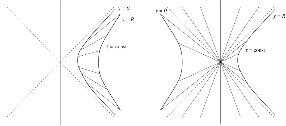
Figure 1: Parts of Minkowski space corresponding to the solution in case 1 (left figure) and case 2 (right figure).

The physical length of the orbifold (obtained by integrating $\sqrt{g_{55}}$ over the coordinate interval $[0,R]$, as usual) is static and in both cases given by

$$R_{\rm phys}=12\left(\frac{1}{V_{1}}+\frac{1}{V_{2}}\right)\;.$$ (5.18)

This is positive due to the conditions (5.16) and (5.17), as it should. In view of eq. (5.15), this leads to

$$H_{i}\sim\frac{1}{R_{\rm phys}}$$ (5.19)

for potentials $V_{i}$ of the some order of magnitude. This relation is quite promising, since it directly relates the Hubble parameters to the size of the additional dimension. We would like to point out that, unlike in the linear case, we did not assume the non–perturbative bulk potential $V$ to depend on the orbifold modulus. Nevertheless, the orbifold size $R_{\rm phys}$ turns out to be time–independent. Moreover, it is fixed by eq. (5.18) in terms of the boundary potentials.

We have already mentioned that the above solution is the only separating solution compatible with our initial assumptions of a stabilized modulus $\phi$ and slow roll of the boundary fields $\phi_{i}$. There is yet another sense in which this solution is unique. Suppose one is interested in solutions where the bulk moduli fields $\beta$ and $\phi$ are constant in time or slowly moving (with a negligible contribution from the bulk potential $V$ to the vacuum energy), the boundary fields are slowly rolling in their potentials $V_{i}$ and the Hubble parameter $H\equiv\dot{\alpha}$ changes only slowly in time. Practically, one can then neglect terms containing $\dot{\beta}$, $\dot{\phi}$, $\dot{\phi_{i}}$ and $\dot{H}$ in the equations of motion. Heuristically, these properties are what one expects from an inflating solution in five dimensions, in analogy with the four–dimensional case. Then, one can show that all solutions with these properties are approximated (in the sense that slow–roll corrections have been neglected) by (5.8)–(5.10). To do this, one does not need the technical assumption of separability that we have used so far. In this sense, we have found the unique solution with boundary inflation in five dimensions.

Can this solution, then, be used as the basis for an inflationary model in five dimensions? We have to keep in mind that we have not solved the equations of motion in general yet, but rather found a specific solution by imposing separability or, equivalently, “reasonable” physical conditions of what an inflationary solution should look like. Therefore, our solution might be very special in the sense that it, perhaps, can only be obtained from a set of initial conditions with measure zero. In other words, the solution could be unstable against small perturbations. We will analyze this question in the following section.

6 Non–linear case: General solution

In this section, we present the general solution. We start with the same setup as in the beginning of section 5. Since we are in the non–linear regime

$$|\epsilon_{i}|\gg 1$$ (6.1)

we can neglect the domain wall potentials. Furthermore, we assume that $\phi$ has been stabilized by the bulk potential $V$ at a point with vanishing potential energy $V(\phi)=0$ (also, as a technical assumption, we have to require the boundary potentials to be independent on $\phi$). Furthermore, the boundary potentials $V_{i}$ should lead to slow roll of the fields $\phi_{i}$. We will, however, not assume separability or slow time evolution of any other field.

It is useful to introduce light–cone coordinates

$$x^{\pm}=\tau\pm y$$ (6.2)

and rewrite the equations of motion (2.20)–(2.23) in terms of these coordinates choosing conformal gauge $\nu=\beta$. Using the simplifications that follow from the above setup, one finds

$$\partial_{+}^{2}\alpha-2\partial_{+}\alpha\partial_{+}\beta+\partial_{+}\alpha^{2} = 0$$ (6.3)

$$\partial_{-}^{2}\alpha-2\partial_{-}\alpha\partial_{-}\beta+\partial_{-}\alpha^{2} = 0$$ (6.4)

$$\partial_{+}\partial_{-}\alpha+3\partial_{+}\alpha\partial_{-}\alpha = 0$$ (6.5)

$$2\partial_{+}\partial_{-}\alpha+\partial_{+}\partial_{-}\beta+3\partial_{+}\alpha\partial_{-}\alpha = 0\;.$$ (6.6)

The boundary conditions (2.26) and (2.27) specialize to

$$e^{-\beta}\alpha^{\prime}\left.\right|_{y=y_{i}}=e^{-\beta}\beta^{\prime}\left.\right|_{y=y_{i}}=\mp\frac{V_{i}}{12}\;,$$ (6.7)

where the upper (lower) sign applies to the boundary at $y=y_{1}$ ($y=y_{2}$). The equations of motion (6.3)–(6.6) are quite similar (although not identical) to those of two–dimensional dilaton gravity [70] with vanishing cosmological constant. In fact, (6.3)–(6.6) can be obtained from the two–dimensional action

$$S_{2}=-\int\sqrt{-g_{2}}e^{3\alpha}\left[R_{2}-24\,\partial_{a}\alpha\partial^{a}\alpha\right]$$ (6.8)

with the two–dimensional metric in conformal gauge given by $g_{ab}=e^{2\beta}\eta_{ab}$. Here we have used indices $a,b,\dots=0,5$ for the space $(\tau,y)$. Using the methods of ref. [70], we can find the following general solution of (6.3)–(6.6)

$$\begin{array}[]{lllllll}\alpha&=&\frac{1}{3}\ln u&,&\beta&=&w-\frac{1}{3}\ln u\\ u&=&u_{+}(x^{+})+u_{-}(x^{-})&,&w&=&w_{+}(x^{+})+w_{-}(x^{-})\end{array}$$ (6.9)

where $u$ and $w$ are free fields, as indicated. The “left– and right–movers” $u_{\pm}(x^{\pm})$ and $w_{\pm}(x^{\pm})$ are not completely independent but, rather, subject to certain relations that originate from the constraint equations (6.3) and (6.4). Three cases can be distinguished

• Case 1: If $\partial_{+}u_{+}\neq 0$ and $\partial_{-}u_{-}\neq 0$ then

  $$w_{\pm}=\frac{1}{2}\ln(\partial_{\pm}u_{\pm})+C_{\pm}\;.$$ (6.10)

• Case 2: If $\partial_{+}u_{+}\neq 0$ and $\partial_{-}u_{-}=0$ then

  $$w_{+}=\frac{1}{2}\ln(\partial_{+}u_{+})+C_{+}\;.$$ (6.11)

  and $w_{-}$ is arbitrary.

• Case 3: If $\partial_{+}u_{+}=0$ and $\partial_{-}u_{-}\neq 0$ then

  $$w_{-}=\frac{1}{2}\ln(\partial_{-}u_{-})+C_{-}\;.$$ (6.12)

  and $w_{+}$ is arbitrary.

Here $C_{\pm}$ are arbitrary integration constants. In each of the three cases, we still have two arbitrary functions at our disposal. While this constitutes the most general solution of the equations of motion (6.3)–(6.6), we have not yet taken into account the boundary conditions (6.7). As we will see, this determines one of the functions and imposes a periodicity constraint on the other one. Before we come to that, we observe that in case 1 we have the relation

$$\beta=2\alpha+\frac{1}{2}\ln(9\partial_{+}\alpha\partial_{-}\alpha)+C_{+}+C_{-}$$ (6.13)

between the scale factors $\alpha$ and $\beta$. Suppose that we have found a solution with an inflating three–dimensional universe in this case. Neglecting $y$–dependence, the scale factor $\alpha$ is then roughly given by $\alpha\sim H\tau$ where $H$ is the Hubble parameter. In this case, the second term on the right hand side of eq. (6.13) is approximately constant since $\partial_{\pm}\alpha$ should be related to the Hubble parameter. Hence, up to an overall normalization we have $\beta\sim 2\alpha$. This shows that, without assuming any initial fine–tuning, at the end of inflation, the orbifold orbifold has expanded twice as much as the three–dimensional universe. For the reasons discussed at the end of section 3 we, therefore, disregard this possibility. We remark that solving the boundary condition (6.7) for case 1 leads to periodicity constraints in terms of elliptic functions.

Let us now turn to cases 2 and 3. Fortunately, the boundary conditions can be explicitly solved in these cases. We find that $\alpha$ and $\beta$ can be expressed in terms of a single real function $f$ as

$$\alpha = \frac{1}{3}\ln f(x^{\pm})$$ (6.14)

$$\beta = \ln\left[\frac{4(f^{\prime}(x^{\pm}))^{1/2}(f^{\prime}(x^{\mp}))^{1/2}}{(\mp V_{1})(f(x^{\mp}))^{2/3}(f(x^{\pm}))^{1/3}}\right]$$ (6.15)

where $f^{\prime}$ denotes the derivative of $f$ and, as usual, $x^{\pm}=\tau\pm y$. The function $f$ should have the periodicity property

$$f(x+2R)=\left[e^{\mp 2RK}(f(x))^{-1/3}+\tilde{k}\right]^{-3}$$ (6.16)

for all $x$, where

$$K=\frac{1}{R}\ln\left(-\frac{V_{1}}{V_{2}}\right)$$ (6.17)

and $\tilde{k}$ is a constant. The condition (6.16) can be solved in terms of a periodic function $p(x)$ satisfying

$$p(x+2R)=p(x)$$ (6.18)

for all $x$. One finds

$$f(x) = \left[p(x)e^{\mp Kx}+k\right]^{-3}\qquad\mbox{for }K\neq 0$$ (6.19)

$$f(x) = \left[kx+p(x)\right]^{-3}\qquad\qquad\mbox{for }K=0$$ (6.20)

where $k$ is another constant. The upper sign in the above solutions always corresponds to case 2, the lower one to case 3. The definition of $K$, eq. (6.17), shows that the boundary potentials need to have opposite sign for the solution to exist. We are, therefore, in the first case (5.16) of the previous section which is as expected since we have used conformal gauge. We will stick to this case, for simplicity, in the following. The analog of the second case (5.17) can again be obtained by employing a more general coordinate system. Our main conclusions apply to this case as well. Furthermore, the periodic function $p(x)$ and the constant $k$ have to be chosen such that the logarithms in (6.14) and (6.15) are well–defined. Apart from those restrictions, $p(x)$ and $k$ are arbitrary. Eq. (6.14)–(6.20) is the most general solution of the system (6.3)–(6.7) for the cases 2 and 3 which, as we have seen, are the interesting ones in the present context. Since we can more or less freely choose one periodic function we have, in fact, found a very large class of solutions.

Depending on the value of $K$ we have two different possible forms of the function $f$, given in eq. (6.19) and (6.20). The second option, $K=0$, is realized for a vanishing “total potential energy”, $V_{1}+V_{2}=0$. Not surprisingly, in this case, the scale factor $\alpha$ does not inflate but (roughly) shows a power law behaviour, as can be seen by inserting (6.20) into eq. (6.14). Consequently, this second option is only of limited interest to us and we will concentrate on the first one, $K\neq 0$. This case should contain our simple separating solution (5.8)–(5.10) of the previous section. Indeed, if we choose

$$p(x)=\mbox{const}\;,\qquad k=0$$ (6.21)

in eq. (6.19) we recover this solution. What happens for other choices? Let us consider the case $k\neq 0$ and $p(x)$ periodic but otherwise arbitrary. If the argument of the exponential in eq. (6.19) is negative (the case that would lead to an inflationary expansion if $k$ were zero) then, after a very short time $f$ will be approximately constant, unless $k$ is exponentially small. Inserting such an approximately constant $f$ into the expressions (6.14), (6.15) for the scale factors $\alpha$ and $\beta$ shows that the three–dimensional universe becomes static while the orbifold collapses. In the opposite case, where the argument of the exponential is positive, $f$ falls exponentially and, hence, from eq. (6.14), the three–dimensional universe collapses. Either way, to have a stable configuration, we should choose $k=0$. In this case, the scale factors read explicitly

$$\alpha = \pm Kx^{\pm}-\ln p(x^{\pm})$$ (6.22)

$$\beta = Ky+\ln\left[\left(\frac{\mp 12}{V_{1}}\right)\left(\pm K-\frac{p^{\prime}}{p}(x^{\pm})\right)^{1/2}\left(\pm K-\frac{p^{\prime}}{p}(x^{\mp})\right)^{1/2}\frac{(p(x^{\mp}))^{1/2}}{(p(x^{\pm}))^{1/2}}\right]\;.$$ (6.23)

We still have the freedom to choose the periodic function $p$. In the above expressions this function always depends on $x^{\pm}=\tau\pm y$. It, therefore, leads to an oscillation in time with a period $2R$. If we do not want the scale factor $\alpha$ to be significantly effected by this, we should choose the maximum amplitude of $p$ to be sufficiently small, so that $p(x)\simeq$ const. This basically brings us back to our separating solution of the previous section. In essence, this solution is the only one with the desired properties within our setup.

The discussion of this section has revealed two serious problems with the separating solution. First of all, it corresponds to a very specific choice of initial conditions satisfying either $k=0$ or $k$ being exponentially small. All other values of $k$ lead to a collapsing solution. This implies that the case $k=0$, as it stands, corresponds to an unstable situation. A small perturbation that leads to a non–vanishing $k$ will cause a collapse of the universe. The other problem is related to the presence of the periodic function $p$. This function, in fact, encodes the information about the initial inhomogeneity in the orbifold direction and this inhomogeneity survives the whole period of inflation. Of course, this is related to the fact that we are not inflating the orbifold as well which would dilute those inhomogeneities. In the effective four–dimensional linear case of section 4, oscillations of Kaluza–Klein modes were damped away quickly due to the inflationary expansion. Apparently this is no longer true in the non–linear five–dimensional regime. Although those modes do not affect the homogeneity of the three–dimensional universe directly, they could potentially be harmful. For example, eq. (6.22) shows that the “Hubble parameter” $\dot{\alpha}$ contains the periodic function $p(\tau\pm y)$ and consequently oscillates in times. Hence, the modes could have some influence on density fluctuations. Also, their eventual decay into gravitons could leave unwanted relics. In any case, the presence of the function $p$ contradicts somewhat the philosophy of inflation which is supposed to wipe out any initial information.

Is there a possible cure for the stability problem? So far, we did not attempt to stabilize the orbifold in any way. It is clear that this fact is related to the instability that we encounter. While stabilizing the orbifold modulus in a four–dimensional effective theory by simply inventing a potential is relatively straightforward (although understanding the origin of this potential is not), this is not the case in five dimensions. The orbifold size in five dimensions is basically measured by the component $g_{55}$ of the metric. A bulk potential for this component would break general five–dimensional covariance in a very strong way. Also, since $g_{55}$ typically varies across the orbifold it could not be everywhere in a minimum of that potential. Alternatively, one could postulate a bulk potential that only depends on the zero mode of $g_{55}$; that is, the length of the orbifold. This would break general covariance not more seriously than it already is broken by the presence of the orbifold. Suppose such a potential had a minimum for a certain orbifold length $R_{0}$. Could an orbifold modulus stabilized at this minimum be made consistent with our solution? The apparent problem is that the orbifold size is already fixed by eq. (5.18) in terms of the boundary potentials $V_{i}$. There is no obvious reason why $R_{0}$ and $R_{\rm phys}$ should, a priori, coincide. If we assume they do, for some reason, at a certain time, this situation could only be maintained if the boundary inflatons slow–roll in a very specific way so as to leave

$$R_{0}=12\left(\frac{1}{V_{1}(\phi_{1})}+\frac{1}{V_{2}(\phi_{2})}\right)$$ (6.24)

unchanged. This would correspond to a strong correlation of the motion of the two inflatons. Without a detailed analysis of the dynamics, which probably has to be carried out numerically, it is hard to tell whether this would actually happen or whether, instead, the orbifold modulus would start to strongly oscillate around its minimum thereby destroying inflation.

Another way to stabilize the orbifold which avoids these problems is to have a potential for $g_{55}$ on the boundary. Although such a potential cannot appear directly in the boundary actions in (2.1), it may appear in one of the Bianchi identities of heterotic M–theory in five dimensions [27, 71, 68] which contain sources located on the orbifold plane. Particularly, a potential from gaugino condensation would manifest itself in the Bianchi identity. Generically, however, it seems to be difficult to stabilize moduli with potentials from gaugino condensation, in particular in the context of cosmology [64] (see however [72]). In ref. [73] stabilization of the orbifold was achieved by a combination of gaugino condensation and other non–perturbative effects resulting from internally wrapped membranes. Although worth investigating in our context, all those options go beyond our simple toy model and will not be explicitly considered here.

To summarize, while there seem to be interesting solutions with boundary inflation in the non–linear, five–dimensional regime, a closer investigation shows that they have problems related to the stabilization of the orbifold and to inhomogeneities in the orbifold direction that are not diluted. The stabilization problem is, of course, very general and we should not be surprised to encounter it in our cosmological context. It is conceivable that whatever eventually stabilizes the orbifold, also saves our non–linear cosmological solution. While the persistence of the orbifold inhomogeneities appears to be in contradiction with the inflationary paradigm they might, under certain conditions, be acceptable and give rise to interesting predictions. It certainly needs more work to finally decide these questions. Probably one also has to go beyond the simple model we have used in this paper.

Acknowledgments A. L. would like to thank Bruce Bassett, Arshad Momen and Graham Ross for helpful discussions. A. L. is supported by the European Community under contract No. FMRXCT 960090. B. A. O. is supported in part by DOE under contract No. DE-AC02-76-ER-03071 and by a Senior Alexander von Humboldt Award. D. W. is supported in part by DOE under contract No. DE-FG02-91ER40671.

References

- [1] A. Lukas, B. A. Ovrut and D. Waldram, Phys. Lett. B393 (1997) 65.
- [2] N. Kaloper, Phys. Rev. D55 (1997) 3394.
- [3] H. Lü, S. Mukherji, C.N. Pope and K.W. Xu, Phys. Rev. D55 (1997) 7926.
- [4] R. Poppe and S. Schwager, Phys. Lett. B393 (1997) 51.
- [5] F. Larsen and F. Wilczek, Phys. Rev. D55 (1997) 4591.
- [6] A. Lukas, B. A. Ovrut and D. Waldram, Nucl. Phys. B495 (1997) 365.
- [7] A. Lukas, B. A. Ovrut and D. Waldram, Nucl. Phys. B509 (1998) 169.
- [8] H. Lu, S. Mukherji, C.N. Pope, From p–branes to cosmology, CTP-TAMU-65-96, hep-th/9612224.
- [9] E. J. Copeland, R. Easther and D. Wands, Phys. Rev. D56 (1997) 874; Nucl. Phys. B506 (1997) 407.
- [10] S. K. Rama, Phys. Lett. B408 (1997) 91.
- [11] K. Behrndt, Stefan Forste and S. Schwager, Nucl. Phys. B508 (1997) 391.
- [12] C. Park, S. Sin, Phys. Rev. D57 (1998) 4620.
- [13] H. Lu, J. Maharana and S. Mukherj, Phys. Rev. D57 (1998) 2219.
- [14] E.J. Copeland, J. E. Lidsey, D. Wands, Phys. Rev. D57 (1998) 625.
- [15] A. Lukas, B. A. Ovrut and D. Waldram, Phys. Lett. B437 (1998) 291.
- [16] N. Kaloper, I. I. Kogan and K. A. Olive, Phys. Rev. D57 (1998) 7340.
- [17] S. Forste, Phys. Lett. B428 (1998) 44.
- [18] E.J. Copeland, J. E. Lidsey, D. Wands, Phys. Rev. D58 (1998) 043503.
- [19] E.J. Copeland, J. E. Lidsey, D. Wands, Phys. Lett. B443 (1998) 97.
- [20] J. Ellis, N. Kaloper, K. A. Olive and J. Yokoyama, Topological Inflation, CERN-TH-98-217, hep-ph/9807482.
- [21] M. Maggiore and A. Riotto, D–branes and Cosmology, CERN-TH/98-361, hep-th/9811089.
- [22] T. Banks, W. Fischler, L. Motl, Dualities versus Singularities, RU-98-58, hep-th/9811194.
- [23] G. Dvali and S. H. H. Tye, Brane Inflation, NYU-TH-12-98-01, hep-ph/9812483.
- [24] C. Kolda and D. H. Lyth, D–term Inflation and M–theory, LBNL-42577, hep-ph/9812234.
- [25] P. Hořava and E. Witten, Nucl. Phys. B460 (1996) 506.
- [26] P. Hořava and E. Witten, Nucl. Phys. B475 (1996) 94.
- [27] P. Hořava, Phys. Rev. D54 (1996) 7561.
- [28] E. Witten, Nucl. Phys. B471 (1996) 135.
- [29] K. Benakli, Cosmological Solution in M–Theory on , hep-th/9804096.
- [30] K. Benakli, Scales and Cosmological Applications of M–Theory, hep-th/9805181.
- [31] A. Lukas, B.A. Ovrut and Daniel Waldram, Cosmological Solutions of Hořava-Witten Theory, hep-th/9806022.
- [32] A. Lukas, B.A. Ovrut and Daniel Waldram, Cosmology and Heterotic M–theory in Five Dimensions, UPR-825T, hep-th/9812052.
- [33] H. S. Reall, Open and Closed Cosmological Solutions of Hořava–Witten Theory, DAMTP-1998-133, hep-th/9809195.
- [34] J. L. F. Barbon, I.I. Kogan and E. Rabinovici, On stringy thresholds in SYM/AdS thermodynamics, CERN-TH-98-206,hep-th/9809033.
- [35] S. A. Abel, J. L. F. Barbon, I.I. Kogan and E. Rabinovici, String thermodynamics in D–brane backgrounds, CERN-TH-98-375, hep-th/9902058.
- [36] A. Hanany and A. Zafferoni, J. High Energy Phys. 05 (1998) 001.
- [37] A. Hanany and A. M. Uranga, J. High Energy Phys., 05 (1998) 013.
- [38] G. Aldazabal, A. Font, L.E. Ibanez and G. Violero, Nucl. Phys. B536 (1998) 29.
- [39] J. Lykken, E. Poppitz and S. P. Trivedi, Branes with GUTs and supersymmetry breaking, UCSD-PTH-98-16, hep-th/9806080.
- [40] Z. Kakushadze and S. H. H. Tye, Phys. Rev. D58 (1998) 126001.
- [41] C. Burgess, L.E. Ibanez and F. Quevedo, Strings at the Intermediate Scale or is the Fermi Scale Dual to the Planck Scale?, FTUAM-98-21, hep-ph/9810535.
- [42] A. Lukas, B. A. Ovrut, K.S. Stelle and D. Waldram, The Universe as a Domain Wall, UPR-797T, hep-th/9803235, to be published in Phys. Lett. B.
- [43] A. Lukas, B. A. Ovrut, K. S. Stelle and D. Waldram, Heterotic M–theory in Five Dimensions, UPR-804T, hep-th/9806051.
- [44] R. Donagi, A. Lukas, B. A. Ovrut and D. Waldram, Non–perturbative Vacua and Particle Physics in M–theory, UPR-823T, hep-th/9811168.
- [45] R. Donagi, A. Lukas, B. A. Ovrut and D. Waldram, Holomorphic Vector Bundles and Non–perturbative Vacua in M–theory, UPR-827T, hep-th/9901009.
- [46] N. Arkani-Hamed, S. Dimopoulos and Gia Dvali, Phys. Lett. B429 (1998) 263.
- [47] N. Arkani-Hamed, S. Dimopoulos and G. Dvali, Phenomenology, astrophysics and cosmology of theories with submillimeter dimensions and TeV scale quantum gravity, SLAC-PUB-7864, hep-ph/9807344.
- [48] K. R. Dienes, E. Dudas, T. Gherghetta and A. Riotto, Cosmological phase transitions and radius stabilization in higher dimensions, CERN-TH-98-259, hep-ph/9809406.
- [49] D. H. Lyth, Inflation with TeV–scale gravity needs supersymmetry, LANCS-TH/9821, hep-ph/9810320.
- [50] N. Kaloper and A. Linde, Inflation and Large Internal Dimensions, SU-ITP-98-60, hep-th/9811141.
- [51] O. Bertolami and R. Schiappa, Modular Quantum Cosmology, DF-IST-1-98, gr-qc/9810013 and references therein.
- [52] J. Ellis, Z. Lalak, S. Pokorski and W. Pokorski, Five–dimensional Aspects of M–theory and Supersymmetry Breaking, CERN-TH-98-118, hep-ph/9805377.
- [53] J. Ellis, Z. Lalak, S. Pokorski and W. Pokorski, Five–Dimensional Gauged Supergravity and Supersymmetry Breaking in M Theory, CERN-TH-98-359, hep-th/9811133.
- [54] A. Lukas, B. A. Ovrut and D. Waldram, Non–Standard Embedding and Five–Branes in Heterotic M–Theory, UPR-815T, hep-th/9808101.
- [55] E. Witten, Nucl. Phys. B474 (1996) 343.
- [56] R. Donagi, A. Grassi and E. Witten, Mod. Phys. Lett. A11 (1996) 2199.
- [57] A. Lukas, B. A. Ovrut and D. Waldram, The Ten-dimensional Effective Action of Strongly Coupled Heterotic String Theory, UPR-789-T, hep-th/9801087, to be published in Phys. Rev. D.
- [58] A. Lukas, B. A. Ovrut and D. Waldram, On the Four-Dimensional Effective Action of Strongly Coupled Heterotic String Theory, UPR-771T, hep-th/9710208, to be published in Nucl. Phys. B.
- [59] T. Han, J. D. Lykken and R. Zhang On Kaluza–Klein States from Large Extra Dimensions, MADPH-98-1092, hep-ph/9811350.
- [60] M. Gasperini and G. Veneziano, Astroparticle Phys. 1 (1993) 317; for an introduction see for example: G. Veneziano, A simple/short introduction into pre–big–bang physics/cosmology, CERN-TH-98-43, hep-th/9802057.
- [61] For a recent review see: D. H. Lyth and A. Riotto, Particle Physics Models of Inflation and the Cosmological Density Perturbation, LANCS-TH-9720, hep-ph/9807278.
- [62] A. Vilenkin, Phys. Lett. B133 (1983) 177.
- [63] J. Ipser and P. Sikivie, Phys. Rev. D30 (1984) 712.
- [64] R. Brustein and P. J. Steinhardt, Phys. Lett. B302 (1993) 196.
- [65] T. Banks, M. Berkooz, S.H. Shenker, G. Moore and P.J. Steinhardt, Phys.Rev. D52 (1995) 3548.
- [66] H. P. Nilles, M. Olechowski and M. Yamaguchi, Phys. Lett. B415 (1997) 24.
- [67] H. P. Nilles, M. Olechowski and M. Yamaguchi, Supersymmetry Breakdown at a Hidden Wall, BONN-TH-97-10, hep-th/9801030.
- [68] A. Lukas, B. A. Ovrut, K.S. Stelle and D. Waldram, Heterotic M–theory in Five Dimensions, UPR-804T, hep-th/9806051.
- [69] A. Lukas, B.A. Ovrut and Daniel Waldram, Five-branes and supersymmetry breaking in M theory, UPR-828T, hep-th/9901017.
- [70] C. G. Callan, S. B. Giddings, J. A. Harvey and A. Strominger, Phys. Rev. D45 (1992) 1005.
- [71] A. Lukas, B.A. Ovrut and Daniel Waldram, Phys. Rev. D57 (1998) 7529.
- [72] T. Barreiro, B. de Carlos and E.J. Copeland, Phys.Rev. D58 (1998) 083513.
- [73] K. Choi, H. B. Kim and, H. Kim, Moduli stabilization in heterotic M theory, KAIST-TH-98-02A, hep-th/9808122.