UCB-PTH-99/04

hep-th/9902067 LBNL-42813

CERN-TH/99-18

Supergravity Models for $3+1$ Dimensional QCD

Csaba Csáki^a,b,,   Jorge Russo^c,   Konstadinos Sfetsos^d   and John Terning^a,b

^a Department of Physics

University of California, Berkeley, CA 94720, USA

^b Theoretical Physics Group

Ernest Orlando Lawrence Berkeley National Laboratory

University of California, Berkeley, CA 94720, USA

^c Departamento de Física, Universidad de Buenos Aires,

Ciudad Universitaria, Pabellón I, 1428 Buenos Aires.

^d Theory Division, CERN

CH-1211 Geneva 23, Switzerland

ccsaki@lbl.gov, russo@df.uba.ar
sfetsos@mail.cern.ch, terning@alvin.lbl.gov

The most general black M5-brane solution of eleven-dimensional supergravity (with a flat ${\bf R^{4}}$ spacetime in the brane and a regular horizon) is characterized by charge, mass and two angular momenta. We use this metric to construct general dual models of large-$N$ QCD (at strong coupling) that depend on two free parameters. The mass spectrum of scalar particles is determined analytically (in the WKB approximation) and numerically in the whole two-dimensional parameter space. We compare the mass spectrum with analogous results from lattice calculations, and find that the supergravity predictions are close to the lattice results everywhere on the two dimensional parameter space except along a special line. We also examine the mass spectrum of the supergravity Kaluza–Klein (KK) modes and find that the KK modes along the compact D-brane coordinate decouple from the spectrum for large angular momenta. There are however KK modes charged under a $U(1)\times U(1)$ global symmetry which do not decouple anywhere on the parameter space. General formulas for the string tension and action are also given.

[2, 3, 4, 5, 6, 7, 8, 9]

1 Introduction

The conjectured dualities between gauge and string theories [1] have been recently exploited in [2]-[9] to construct and investigate models of pure QCD in 3+1 dimensions, whose main component is the black M5-brane solution of eleven-dimensional supergravity, which near the branes corresponds to an anti-de Sitter (AdS) space. The no-hair theorem implies that the most general model of this kind that can be constructed (i.e. based on a regular geometry with M5-brane charge) is obtained from a rotating black M5-brane parameterized by its charge, mass and two angular momenta. The scope of this paper is to calculate the mass spectrum of scalar modes of this general model in the supergravity approximation, and study its behavior in the parameter space. The parameter space is four dimensional, but the mass parameter can be set to 1 by a choice of mass units; the charge is related to the ’t Hooft coupling $\lambda=g^{2}N$ (where $g$ is the Yang–Mills coupling and $N$ is the number of branes). It is assumed that $\lambda$ is very large so that the radius of curvature is much larger than the string scale; this is necessary for supergravity to be a good approximation to string theory (M theory). In this regime glueball masses are independent of $\lambda$, so what remains is a two-dimensional space spanned by the angular momentum parameters. When one of the angular momenta vanishes, the model reduces to the one angular momentum model examined in Refs. [6, 8]. In our investigation we will use both analytic methods (within the WKB approximation, as developed in Refs. [9, 10]) as well as numerical ones based on Ref. [4].

The static M5-brane has an $SO(5)$ symmetry associated with the internal $S^{4}$. Turning on the angular momentum parameters, this symmetry group breaks down to the Cartan subgroup as $SO(5)\to SO(2)\times SO(2)\sim U(1)\times U(1)$. The spectrum of the supergravity field fluctuations can be organized in representations of $SO(5)$ or $SO(2)\times SO(2)$. The proposal of Refs. [2]-[4] is to identify the $SO(5)$-singlet modes propagating on the Minkowski boundary of the spacetime with large-$N$ QCD glueballs. The dilaton modes correspond to $J^{PC}=0^{++}$ glueballs ($J$, $P$, and $C$ being the spin, parity and charge conjugation quantum numbers). In non-supersymmetric, pure $SU(N)$ Yang–Mills theory, there is no counterpart of the $SO(5)$ global symmetry, so one would expect that at weak Yang–Mills coupling those Kaluza–Klein (KK) particles which transform non-trivially under this group are very massive and decouple. This problem was studied for ${\rm QCD}_{3}$ in [11] where it was shown that the first correction (beyond the $\lambda=\infty$ limit) to the masses of these states does not lead to their decoupling in the case of vanishing angular momenta. A general study for ${\rm QCD}_{3}$ supergravity models with three angular momenta was recently given in [10]. In this paper, using both analytic (within the WKB approximation) and numerical methods, we calculate the spectrum of glueballs and of KK states. We find that the KK modes on $S^{4}$ do not decouple in the large $\lambda$ regime in any region of the two dimensional parameter space (within the supergravity approximation). In contrast, the KK modes on the circle associated with the compact Euclidean time (on the M5-brane worldvolume) decouple in the limit of large angular momentum.

Some interesting effects concerning thermodynamical aspects of rotating D-branes have been recently pointed out in Refs. [12]-[14]. Here we will be considering the slightly different construction of Refs. [2, 6] for zero-temperature QCD, where the Euclidean time parameterizes an internal circle, and the Minkowski time is one of the brane volume coordinates.

2 The Supergravity Model

2.1 The metric

The maximal number of angular momentum parameters for the rotating M5-brane (dictated by the rank of the $SO(5)$ isometry group of rotations of the static M5-brane) is equal to two. This metric was constructed in [15], though the expression given there contains a few minor mistakes which we correct below. The metric of the rotating M5-brane is given by

$$ds_{11}^{2}= f^{-\frac{1}{3}}(-hdt^{2}+dx_{1}^{2}+\ldots+dx_{5}^{2})+\frac{f^{\frac{2}{3}}}{\tilde{h}}dr^{2}+f^{\frac{2}{3}}r^{2}\big{[}(1+\frac{l_{1}^{2}\cos^{2}\theta}{r^{2}}+$$

$$\frac{l_{2}^{2}\sin^{2}\theta\sin^{2}\psi}{r^{2}})d\theta^{2}+(1+\frac{l_{2}^{2}\cos^{2}\psi}{r^{2}})\cos^{2}\theta d\psi^{2}-2\frac{l_{2}^{2}}{r^{2}}\cos\theta\sin\theta\cos\psi\sin\psi d\theta d\psi$$

$$-4m\frac{\cosh\delta}{r^{5}\Delta f}dt(l_{1}\sin^{2}\theta d\varphi_{1}+l_{2}\cos^{2}\theta\sin^{2}\psi d\varphi_{2})+\frac{4ml_{1}l_{2}\cos^{2}\theta\sin^{2}\theta\sin^{2}\psi}{r^{5}\Delta f}d\varphi_{1}d\varphi_{2}$$

$$+\sin^{2}\theta(1+\frac{l_{1}^{2}}{r^{2}}+\frac{2ml_{1}^{2}\sin^{2}\theta}{r^{5}\Delta f})d\varphi_{1}^{2}+\cos^{2}\theta\sin^{2}\psi(1+\frac{l_{2}^{2}}{r^{2}}+\frac{2ml_{2}^{2}\cos^{2}\theta\sin^{2}\psi}{r^{5}\Delta f})d\varphi_{2}^{2}\Big{]},$$

where

$$\Delta=1+\frac{l_{1}^{2}}{r^{2}}\cos^{2}\theta+\frac{l_{2}^{2}}{r^{2}}(\sin^{2}\theta+\cos^{2}\theta\cos^{2}\psi)+\frac{l_{1}^{2}l_{2}^{2}}{r^{4}}\cos^{2}\theta\cos^{2}\psi\ ,$$ (2.2)

$$f=1+\frac{2m\sinh^{2}\alpha}{\Delta r^{3}}\ ,$$ (2.3)

$$h=1-\frac{2m}{\Delta r^{3}}\ ,$$ (2.4)

$$\tilde{h}=\frac{1+\frac{l_{1}^{2}}{r^{2}}+\frac{l_{2}^{2}}{r^{2}}+\frac{l_{1}^{2}l_{2}^{2}}{r^{4}}-\frac{2m}{r^{3}}}{\Delta}\ .$$ (2.5)

The horizon is located at $r=r_{H}$, where $r_{H}$ is the largest real root of

$$\big{(}r^{2}+l_{1}^{2}\big{)}\big{(}r^{2}+l_{2}^{2}\big{)}-2mr=0\ .$$ (2.6)

One can obtain the following formulas for the ADM mass, entropy and angular momentum:

$$M_{\rm ADM} = {V_{5}V(\Omega_{4})\over 4\pi G_{N}}\ 2m(1+{3\over 4}\sinh^{2}\alpha)\ ,\ \ \ \ \ V(\Omega_{4})={8\pi^{2}\over 3}\ ,$$ (2.7)

$$S = {V_{5}V(\Omega_{4})\over 4G_{N}}\ 2m\ r_{H}\cosh\alpha\ ,$$ (2.8)

$$J_{1,2} = {V_{5}V(\Omega_{4})\over 4\pi G_{N}}\ m\ l_{1,2}\cosh\alpha\ ,$$ (2.9)

$$G_{N}={\kappa_{11}^{2}\over 8\pi}=2^{4}\pi^{7}l_{\rm P}^{9}\ ,$$ (2.10)

where $G_{N}$ is Newton’s constant in 11 dimensions, and $l_{\rm P}$ is the 11 dimensional Planck length. The parameter $\alpha$ is related to the (magnetic) charge $N$ and $m$ by

$$\sinh^{2}\alpha={1\over 2}\left(\sqrt{(\pi Nl_{\rm P}^{3}/m)^{2}+1}-1\right)\ .$$ (2.11)

The Hawking temperature and angular velocities are given by

$$T_{H}={3r_{H}^{4}+(l_{1}^{2}+l_{2}^{2})r_{H}^{2}-l_{1}^{2}l_{2}^{2}\over 8\pi mr_{H}^{2}\cosh\alpha}\ ,\ \ \ \ \ \Omega_{1,2}={l_{1,2}\over\cosh\alpha\ (r_{H}^{2}+l_{1,2}^{2})}\ .$$ (2.12)

These quantities satisfy the first law of black hole thermodynamics:

$$dM_{\rm ADM}=T_{H}dS+\Omega_{1}dJ_{1}+\Omega_{2}dJ_{2}\ .$$ (2.13)

Let us now go to Euclidean space $\tau=-it$, $l_{1,2}\to il_{1,2}$, and take the field theory limit as in [1, 6]:

$$r=U^{2}l_{\rm P}^{3},\ \ \ \ 2m=U_{0}^{6}l_{\rm P}^{9},\ \ \ \ l_{1,2}=a_{1,2}^{2}l_{\rm P}^{3}\ ,$$ (2.14)

so that $2m\sinh^{2}\alpha\to\pi Nl_{\rm P}^{3}$. We obtain the metric

$$ds_{11}^{2} = \frac{\Delta^{\frac{1}{3}}U^{2}l_{\rm P}^{2}}{(\pi N)^{\frac{1}{3}}}\Big{[}(1-\frac{U_{0}^{6}}{U^{6}\Delta})d\tau^{2}+dx_{1}^{2}+\ldots dx_{5}^{2}\Big{]}+l_{\rm P}^{2}\frac{\Delta^{\frac{1}{3}}(\pi N)^{\frac{2}{3}}4dU^{2}}{U^{2}[(1-\frac{a_{1}^{4}}{U^{4}})(1-\frac{a_{2}^{4}}{U^{4}})-\frac{U_{0}^{6}}{U^{6}}]}+$$ (2.15)

$$\frac{l_{\rm P}^{2}(\pi N)^{\frac{2}{3}}}{\Delta^{\frac{2}{3}}}\Big{[}\Delta_{1}d\theta^{2}+\Delta_{2}\cos^{2}\theta d\psi^{2}+2\frac{a_{2}^{4}}{U^{4}}\cos\theta\sin\theta\cos\psi\sin\psi d\theta d\psi$$

$$-\frac{2U_{0}^{3}}{U^{4}(\pi N)^{\frac{1}{2}}}(a_{1}^{2}\sin^{2}\theta d\tau d\varphi_{1}+a_{2}^{2}\cos^{2}\theta\sin^{2}\psi d\tau d\varphi_{2})+\sin^{2}\theta(1-\frac{a_{1}^{4}}{U^{4}})d\varphi_{1}^{2}+$$

$$\cos^{2}\theta\sin^{2}\psi(1-\frac{a_{2}^{4}}{U^{4}})d\varphi_{2}^{2}\Big{]},$$

where

$$\Delta_{1}=1-\frac{a_{1}^{4}\cos^{2}\theta}{U^{4}}-\frac{a_{2}^{4}\sin^{2}\theta\sin^{2}\psi}{U^{4}}\ ,$$ (2.16)

$$\Delta_{2}=1-\frac{a_{2}^{4}\cos^{2}\psi}{U^{4}}\ ,$$ (2.17)

$$\Delta=1-\frac{a_{1}^{4}\cos^{2}\theta}{U^{4}}-\frac{a_{2}^{4}(\sin^{2}\theta+\cos^{2}\theta\cos^{2}\psi)}{U^{4}}+\frac{a_{1}^{4}a_{2}^{4}\cos^{2}\theta\cos^{2}\psi}{U^{8}}\ .$$ (2.18)

Note that the component $g_{\varphi_{1}\varphi_{2}}$ vanishes in the field theory limit, and so do the last terms in $g_{\varphi_{1}\varphi_{1}}$ and $g_{\varphi_{2}\varphi_{2}}$.

The coordinate $\tau$ describes a circle of radius $R_{0}$, where $R_{0}$ is related to the Hawking temperature $T_{H}$ by $R_{0}=(2\pi T_{H})^{-1}$, with

$$T_{H}={3u_{0}\over 2\pi A}\ ,\ \ \ \$$ (2.19)

$$A=\frac{u_{H}^{4}u_{0}^{4}}{u_{H}^{8}-\frac{1}{3}(a_{1}^{4}+a_{2}^{4})u_{H}^{4}-\frac{1}{3}a_{1}^{4}a_{2}^{4}}={3u_{0}^{4}u_{H}^{2}\over(u_{H}^{2}-u_{IH}^{2})(u_{H}^{2}-u_{1}^{2})(u_{H}^{2}-u_{2}^{2})}\ ,$$ (2.20)

where we have introduced the coordinate $u$ by $U=2(\pi N)^{1/2}u$, and rescaled $a_{1,2}\to$ $2(\pi N)^{1/2}a_{1,2}$. The constants $u_{H}^{2},u_{IH}^{2},u_{1}^{2},u_{2}^{2}$ represent the four different solutions for $u^{2}$ of the equation

$$(u^{4}-a_{1}^{4})(u^{4}-a_{2}^{4})-u_{0}^{6}u^{2}=0~{}.$$ (2.21)

There are two positive ($u_{H}^{2}$, $u_{IH}^{2}$, $u_{H}^{2}>u_{IH}^{2}$), and two negative (or complex) solutions ($u_{1}^{2},u_{2}^{2}$), with $u_{H}^{2}$ and $u^{2}_{IH}$ representing the outer and inner horizons respectively. When $a_{1}=a_{2}=a$, the equation simplifies to

$$u^{4}-a^{4}=\pm u_{0}^{3}u~{},$$ (2.22)

where the signs $\pm$ corresponds to the inner and outer horizons. From Eq. (2.22) one sees that when $a\gg u_{0}$ the two positive solutions get closer to each other, thus the inner horizon approaches the outer horizon.

The gauge coupling $g_{4}^{2}$ in the $3+1$ dimensional Yang–Mills theory is given by the ratio between the periods of the eleven-dimensional coordinates $x_{5}$ and $\tau$, i.e.

$$\tau=R_{0}\theta_{2},\ \ \ x_{5}={g_{4}^{2}\over 2\pi}R_{0}\theta_{1}=\frac{\lambda}{N}R_{0}\theta_{1}\ ,\ \ \ \ \ \theta_{1,2}=\theta_{1,2}+2\pi\ ,$$ (2.23)

where $\lambda\equiv{g_{4}^{2}N\over 2\pi}$ is the ’t Hooft coupling. Dimensional reduction in $\theta_{1}$ gives the type IIA metric representing the field theory limit of the rotating D4-brane metric with two angular momentum parameters:

$$ds_{\rm IIA}^{2} = \frac{2\pi\lambda A}{3u_{0}}u\Delta^{\frac{1}{2}}\big{[}4u^{2}(-dx_{0}^{2}+dx_{1}^{2}+dx_{2}^{2}+dx_{3}^{2})+\frac{4A^{2}}{9u_{0}^{2}}u^{2}(1-\frac{u_{0}^{6}}{u^{6}\Delta})d\theta_{2}^{2}+$$ (2.24)

$$+\frac{4du^{2}}{u^{2}((1-\frac{a_{1}^{4}}{u^{4}})(1-\frac{a_{2}^{4}}{u^{4}})-\frac{u_{0}^{6}}{u^{6}})}+\frac{\Delta_{1}}{\Delta}d\theta^{2}+\frac{\Delta_{2}}{\Delta}\cos^{2}\theta d\psi^{2}$$

$$+2\frac{a_{2}^{4}}{u^{4}\Delta}\cos\theta\sin\theta\cos\psi\sin\psi d\theta d\psi+\sin^{2}\theta\frac{(1-\frac{a_{1}^{4}}{u^{4}})}{\Delta}d\varphi_{1}^{2}+\cos^{2}\theta\sin^{2}\psi\frac{(1-\frac{a_{2}^{4}}{u^{4}})}{\Delta}d\varphi_{2}^{2}$$

$$-\frac{4Au_{0}^{2}}{3u^{4}\Delta}(a_{1}^{2}\sin^{2}\theta d\theta_{2}d\varphi_{1}+a_{2}^{2}\cos^{2}\theta\sin^{2}\psi d\theta_{2}d\varphi_{2})\Big{]}\ ,$$

where the dilaton field is given by

$$e^{2\Phi}=\frac{8\pi A^{3}\lambda^{3}u^{3}\Delta^{\frac{1}{2}}}{27u_{0}^{3}N^{2}}\ .$$ (2.25)

In these coordinates, the metric is independent of $N$, and the string coupling is of order $1/N$, as expected. The ’t Hooft coupling $\lambda$ appears as an overall factor of the metric. For $u_{0}\neq 0$, curvature invariants have a finite value at the horizon, and they are suppressed by inverse powers of $\lambda$.

The metric (2.24) has a $U(1)^{3}$ isometry associated with translations in $\theta_{2},\varphi_{1},\varphi_{2}$. This should appear as a global symmetry in the corresponding dual Yang–Mills theory. Since the pure $SU(N)$ QCD has no such symmetries, one may expect that states which have charges with respect to $U(1)^{3}$ have a large mass compared to the glueball masses. In Section 4 we calculate the different mass spectra and investigate this possibility.

2.2 String tension and action

The string tension is given by $1/2\pi$ times the coefficient of $\sum dx_{i}^{2}$, evaluated at the horizon, at the angles where it takes its minimum value [2, 6]. This follows by minimizing the Nambu–Goto action of the string configuration. The absolute minimum occurs at $\theta=\psi=0$ or $\pi$. We obtain

$$\sigma={4\over 3}\lambda Au_{0}^{2}\ .$$ (2.26)

String excitations should have masses of order $\sigma^{1/2}$. The spin $\leq 2$ glueballs that remain in the supergravity approximation – whose masses are determined from the Laplace equation – have masses which are independent of $\lambda$.

In the field theory limit, the free energy $F$ ($={\rm Action}\times T_{H}$) takes the simple form

$$\ F=E-T_{H}S-\Omega_{1}J_{1}-\Omega_{2}J_{2}=-{V_{5}\over 3\pi^{3}}\ N^{3}\ u_{0}^{6}\ ,$$ (2.27)

where $E=M_{\rm ADM}-M_{\rm extremal}\ ,M_{\rm extremal}=M_{\rm ADM}(u_{0}=0)$. Using that the M5-brane coordinate $x_{5}$ is compactified on a circle with radius $R_{0}\lambda/N$, one has the relation

$$V_{5}={V_{4}\lambda\over T_{H}N}\ .$$ (2.28)

Expressing $u_{0}$ in terms of the string tension (2.26) we obtain the intriguing relation

$$-{{\rm Action}\over V_{4}}={1\over 12\pi}{N^{2}\over\lambda}\sigma^{2}\ ,$$ (2.29)

that generalizes the result found in [8] for the case of one angular momentum. Thus, in terms of the string tension, the action is independent of $a_{1,2}$. It would be very interesting to have a derivation of (2.29) from the Yang–Mills side as a non-perturbative contribution to the partition function (related to the expectation value of the gluon condensate $\langle{1\over 4g_{YM}^{2}}{\rm Tr\ }F_{\mu\nu}^{2}(0)\rangle$).

2.3 The supersymmetric limit $u_{0}=0$

Metrics of rotating branes with non-extremality parameter $m=0$ greatly simplify upon introducing Cartesian-type coordinates [6]. For the extremal ($m=0$) M5-brane metric (2.1), one introduces [13]

$$y_{1}=\sqrt{r^{2}+l_{1}^{2}}\sin\theta\cos\varphi_{1}\ ,\ \ \ \ \ \ \ \ \ \ \ y_{2}=\sqrt{r^{2}+l_{1}^{2}}\sin\theta\sin\varphi_{1}\ ,\ \ \ \$$

$$y_{3}=\sqrt{r^{2}+l_{2}^{2}}\cos\theta\sin\psi\cos\varphi_{2}\ ,\ \ \ \ y_{4}=\sqrt{r^{2}+l_{2}^{2}}\cos\theta\sin\psi\sin\varphi_{2}\ ,\ \ \ \$$

$$y_{5}=r\cos\theta\cos\psi\ .$$ (2.30)

Using these coordinates we obtain

$$ds^{2}_{\rm IIA}=f^{-1/2}\big{[}-dx_{0}^{2}+\sum_{i=1}^{4}dx_{i}^{2}\big{]}+f^{1/2}\sum_{j=1}^{5}dy_{j}^{2}\ ,$$ (2.31)

where $f$ is obtained from Eq. (2.3) by taking the limit $\alpha\to\infty,\ m\to 0$ at fixed $N$ using (2.11): $f=1+{\pi Nl_{\rm P}^{3}\over\Delta r^{3}}$, with $r$, $\theta,\ \psi$ expressed in terms of $y_{j}$ by Eq. (2.30). In this limit the BPS bound is saturated, $M_{\rm ADM}={\rm const}\ N$. It can be shown that the function $f(y_{j})$ satisfies the equation $\partial_{j}\partial^{j}f=0$, i.e. it is a harmonic function in the 5-space parameterized by $y_{j}$. The metric (2.31) has unbroken supersymmetries, which can also be understood by interpreting the metric (2.31) as a multicenter distribution of BPS D4-branes, by constructing the harmonic function $f$ as a linear superposition of harmonic functions corresponding to each D4-brane [13, 16].

The field theory limit of (2.31) can be obtained by replacing $f\to f-1$, and properly rescaling coordinates. Alternatively, we can return to the metric (2.24) written in spherical coordinates, and set $u_{0}=0$. The resulting metric has a curvature singularity in $u=a_{1}$ (we are assuming $a_{1}>a_{2}>0$), which cannot be removed by any choice of periodicity in the $\tau$ coordinates (the horizon region of the extremal $u_{0}=0$ metric is not a Rindler space). Because of the singularity, the supergravity approximation breaks down in the $u_{0}=0$ case; in order to understand the corresponding supersymmetric gauge theory, one needs to understand the full string theory. At the supergravity level, it is meaningless to associate a temperature to this metric.

One can have control over the string-theory corrections if we regularize the metric by taking $u_{0}\neq 0$ and consider the limit of small $u_{0}$ (or equivalently, $a_{1,2}/u_{0}$ large). For any value of $a_{1,2}/u_{0}$, one can choose $\lambda$ sufficiently large so that all curvature invariants are arbitrarily small. This is the technique used in the next section when discussing the large $a_{1,2}/u_{0}$ limit. Note that in this limit $T_{H}\to\infty$. In this theory, all fermions—which have masses ${\cal O}(T_{H})$—decouple. On the other hand, the spectrum of the $u_{0}=0$ theory must be supersymmetric with the usual degeneracy between fermions and bosons. The supersymmetric $u_{0}=0$ theory cannot coincide with the theory obtained by taking the limit $u_{0}\to 0$ (in the fashion described above), since the latter theory does not have fermions in the spectrum. Nevertheless, since the corresponding background metrics are essentially the same (at $a_{1,2}\gg u_{0}$) it is possible that a part of the structure of the theory with $a_{1}/u_{0}\gg 1$ may be dictated by the structure of the $u_{0}=0$ supersymmetric model. We shall return to this point in our conclusions.

3 Glueballs and the Related KK Modes

The $0^{++}$ glueballs are related to spherically symmetric modes of the dilaton fluctuations, of the form

$$\Psi=\phi(u)e^{ik\cdot x}\ ,$$ (3.1)

where $M^{2}=-k^{2}$ [2]. The differential equation determining the mass eigenvalues is obtained by substituting this into the dilaton equation of motion

$${1\over\sqrt{g}}\partial_{\mu}\left[e^{-2\Phi}\sqrt{g}g^{\mu\nu}\partial_{\nu}\Psi\right]=0\ ,$$ (3.2)

using the background metric (2.24), and the formula

$$\sqrt{g}=C\ u^{9}\Delta\cos^{2}\theta\sin\theta\sin\psi\ ,\ \ \ \ \ C={1\over 2\pi\lambda}\left({4\pi\lambda A\over 3u_{0}}\right)^{6}\ .$$ (3.3)

In addition to the $0^{++}$ glueballs we consider particles with non-vanishing $U(1)$ charge associated with the circle parameterized by $\theta_{2}$. The corresponding solutions of (3.2) will be of the form

$$\Psi=\phi(u)e^{ik\cdot x}e^{in\theta_{2}}\ .$$ (3.4)

We will show both analytically (within the WKB approximation) and numerically that these states do decouple for a particular range of parameters. We will also consider the KK states associated with the $l=1$ modes of the $S^{4}$. For the static ($a_{1}=a_{2}=0$) M5 metric, these transform in the ${\bf 5}$ representation of $SO(5)$. After introducing angular momentum, this decomposes into ${\bf(2,1)}\oplus{\bf(1,2)}\oplus{\bf(1,1)}$ of the Cartan subgroup $SO(2)\times SO(2)$. According to this decomposition, the corresponding solutions of (3.2) for the two doublets will be given by

$$\Psi=\phi(u)e^{ik\cdot x}\sin\theta\pmatrix{\cos\varphi_{1}\cr\sin\varphi_{1}}\ ,$$ (3.5)

$$\Psi=\phi(u)e^{ik\cdot x}\cos\theta\sin\psi\pmatrix{\cos\varphi_{2}\cr\sin\varphi_{2}}\ ,$$ (3.6)

whereas for the singlet it is of the form

$$\Psi=\phi(u)e^{ik\cdot x}\cos\theta\cos\psi\ .$$ (3.7)

In ordinary (finite $\lambda,N$) Yang–Mills theory there is no $SO(2)\times SO(2)$ symmetry, so one would expect that at least the states which transform non-trivially under $SO(2)\times SO(2)$ become very massive and decouple in the weak-coupling limit. It is clear that the singlet state (3.7) should also decouple. If it did not decouple at small $\lambda$, it would then be represented by some (gluon field) operator in the gauge theory. In the zero angular momentum case, this state combines with the other four components to form a multiplet (a ${\bf 5}$) of $SO(5)$. Thus the singlet state cannot correspond to a purely gluonic operator (since the gluon field is a singlet under $SO(5)$), and must decouple.

Finally, we shall also consider $0^{-+}$ glueballs, which couple to the operator $\tilde{\cal O}_{4}={\rm Tr}\ F\tilde{F}$. On the D4-brane worldvolume, the field that couples to this operator is the R–R 1-form $A_{\mu}$, which satisfies the equation of motion

$$\partial_{\nu}\big{[}\sqrt{g}g^{\mu\rho}g^{\nu\sigma}(\partial_{\rho}A_{\sigma}-\partial_{\sigma}A_{\rho})\big{]}=0\ ,\qquad\mu,\nu=1,\dots,10\ .$$ (3.8)

Finding angular-independent solutions is complicated, because of the non-diagonal components of the metric. The metric becomes diagonal in the two opposite limits $a_{1,2}\ll u_{0}$ and $a_{1,2}\gg u_{0}$. In these cases one can consider solutions of the form

$$A_{\rm\theta_{2}}=\chi_{\theta_{2}}(u)\ e^{ik\cdot x}\ ,\ \ \ \ \ \ \ A_{\mu}=0\ \ {\rm if}\ \ \mu\neq\theta_{2}\ .$$ (3.9)

In the following we will first present the mass spectra of these states obtained in the WKB approximation, and then the same spectra obtained by using numerical methods. We present tables for each state comparing the WKB with the numerical results and find that they are in a very good agreement. We also compare them to the lattice results for the glueball states which were computed for $N=3$ and small $\lambda$.

3.1 Mass spectrum in the WKB approximation

In the following we use the WKB approach of [10] (which generalizes the WKB approach of [9]) to calculate the different mass spectra (including KK modes) in the present case of QCD₄ with two angular momenta. Consider differential equations of the form

$$\partial_{\rho}\left(f(\rho)\partial_{\rho}\phi\right)+\left(M^{2}h(\rho)+p(\rho)\right)\phi=0\ ,$$ (3.10)

where $M$ represents a mass parameter, and $f(\rho)$, $h(\rho)$ and $p(\rho)$, $\rho\in[\rho_{H},\infty)$, are three arbitrary functions which are independent of $M$ and have the following behavior:

$$f\approx f_{1}(\rho-\rho_{H})^{s_{1}}\ ,\quad h\approx h_{1}(\rho-\rho_{H})^{s_{2}}\ ,\quad p\approx p_{1}(\rho-\rho_{H})^{s_{3}}\ ,\qquad{\rm as}\quad\rho\to\rho_{H}\ ,$$ (3.11)

$$f\approx f_{2}\rho^{r_{1}}\ ,\quad h\approx h_{2}\rho^{r_{2}}\ ,\quad p\approx p_{2}\rho^{r_{3}}\ ,\qquad{\rm as}\quad\rho\to\infty\ ,$$ (3.12)

where $r_{1,2,3}$, $s_{1,2,3}$, $f_{1,2}$, $h_{1,2}$ and $p_{1,2}$ are (real) numerical constants. For large masses $M$, the WKB method can be applied to obtain the approximate spectrum. One finds [10]

$$M^{2}={\pi^{2}\over\xi^{2}}\ m\left(m+\Big{(}\!-\!1+{\alpha_{2}\over\alpha_{1}}+{\beta_{2}\over\beta_{1}}\Big{)}\right)\ +\ {\cal O}(m^{0})\ ,\qquad m\geq 1\ .$$ (3.13)

where

$$\xi=\int_{\rho_{H}}^{\infty}d\rho\ \sqrt{h\over f}\ ,$$ (3.14)

is a constant which scales like a length, and

$$\alpha_{1}=s_{2}-s_{1}+2\ ,\qquad\beta_{1}=r_{1}-r_{2}-2\ ,$$ (3.15)

$$\alpha_{2}=|s_{1}-1|\quad{\rm or}\quad\alpha_{2}=\sqrt{(s_{1}-1)^{2}-4{p_{1}\over f_{1}}}\ \ ({\rm if}\ s_{3}-s_{1}+2=0)\ ,$$

$$\beta_{2}=|r_{1}-1|\quad{\rm or}\quad\beta_{2}=\sqrt{(r_{1}-1)^{2}-4{p_{2}\over f_{2}}}\ \ ({\rm if}\ r_{1}-r_{3}-2=0)\ .$$ (3.16)

Consistency requires that $\alpha_{1}$ and $\beta_{1}$ are strictly positive numbers whereas $s_{3}-s_{1}+2$ and $r_{1}-r_{3}-2$ can be either positive or zero. Typically the validity of the WKB approximation requires that the quantum number $m$ be much larger than 1 (for precise conditions see [10]).

3.1.1 Masses of the $0^{++}$ glueballs

The masses of the $0^{++}$ glueballs are determined from the differential equation (3.2) with the ansatz (3.1). Introducing $\rho=u^{2}$ one gets Eq. (3.10) with

$$f(\rho)=(\rho^{2}-b_{1}^{2})(\rho^{2}-b_{2}^{2})-\rho_{0}^{3}\rho\equiv(\rho-\rho_{H})(\rho-\rho_{1})(\rho-\rho_{2})(\rho-\rho_{3})\ ,$$

$$h(\rho)={\rho\over 4}\ ,\ \ \ \ p(\rho)=0\ .$$ (3.17)

This gives for the various constants

$$s_{1}=1\ ,\quad s_{2}=0\ ,\quad r_{1}=4\ ,\quad r_{2}=1\ ,$$

$$\alpha_{1}=1\ ,\quad\alpha_{2}=0\ ,\quad\beta_{1}=1\ ,\quad\beta_{2}=3\ .$$ (3.18)

Using (3.13) one obtains the following mass spectrum

$$M^{2}={\pi^{2}\over\xi^{2}}\ m(m+2)+{\cal O}(m^{0})\ ,\qquad m\geq 1\ ,$$

$$\xi={1\over 2}\int_{\rho_{H}}^{\infty}{d\rho\ \sqrt{\rho}\over\sqrt{(\rho-\rho_{H})(\rho-\rho_{1})(\rho-\rho_{2})(\rho-\rho_{3})}}\ ,$$ (3.19)

This formula implies that mass ratios between resonances are, in the WKB approximation, independent of the angular momentum parameters $b_{1},b_{2}$. This is similar to ${\rm QCD}_{3}$, where the general rotating D3-brane solution with three angular momenta parameters was used [10]. As in [10], the WKB approximation breaks down in the region near $b_{1}=b_{2}$, $u_{0}=0$.

3.1.2 The KK modes on the circle

For the KK modes with non-vanishing $U(1)$ charge corresponding to the periodic variable $\theta_{2}$ we look for solutions of (3.2) with the ansatz (3.4). In this case we obtain Eq. (3.10) with $M^{2}$ replaced by $M^{2}-4\pi^{2}n^{2}T_{H}^{2}$ and

$$f(\rho)=(\rho^{2}-b_{1}^{2})(\rho^{2}-b_{2}^{2})-\rho_{0}^{3}\rho\ ,$$

$$h(\rho)={\rho\over 4}\ ,\qquad p(\rho)=-{\pi^{2}n^{2}\rho_{0}^{3}T_{H}^{2}\rho^{2}\over f(\rho)}\ .$$ (3.20)

This gives for the various constants

$$s_{1}=1\ ,\quad s_{2}=0\ ,\quad s_{3}=-1\ ,\quad r_{1}=4\ ,\quad r_{2}=1\ ,\quad r_{3}=-2\ ,$$

$$\alpha_{1}=1\ ,\quad\alpha_{2}={2\pi n\rho_{0}^{3/2}\rho_{H}T_{H}\over(\rho_{H}-\rho_{1})(\rho_{H}-\rho_{2})(\rho_{H}-\rho_{3})}\ ,\quad\beta_{1}=1\ ,\quad\beta_{2}=3\ .$$ (3.21)

Using (2.19) and (2.20) we see that $\alpha_{2}=n$. Then (3.13) (with $M^{2}\to M^{2}-4\pi^{2}n^{2}T_{H}^{2}$) gives the following mass spectrum

$$M^{2}=4\pi^{2}n^{2}T_{H}^{2}\ +\ {\pi^{2}\over\xi^{2}}\ m(m+2+n)+{\cal O}(m^{0})\ ,\qquad m\geq 1\ .\\$$

We would like to examine the way that these states decouple in two limiting cases. First consider the case with $b_{1}\gg\rho_{0}\ {\rm and}\ b_{2}$. Then we see from (2.19) that

$$T_{H}\simeq{b_{1}^{2}\over\pi\rho_{0}^{3/2}}~{}.$$ (3.22)

On the other hand, in the same limit,

$$\xi\simeq{1.31\over b_{1}^{1/2}}~{}.$$ (3.23)

Therefore the ratios of the masses of the glueballs to those of the $U(1)$ charged particles behave as

$${M_{\rm glueb.}\over M_{\rm circ.}}\simeq 1.20{\sqrt{m(m+2)}\over n}\left({\rho_{0}\over b_{1}}\right)^{3/2}\ ,\qquad{\rm for}\quad b_{1}\gg\rho_{0}\ {\rm and}\ b_{2}\ .$$ (3.24)

Hence, the KK modes on the circle decouple with a power law. Now consider the case $b_{1}=4b_{2}\gg\rho_{0}$. Then

$$T_{H}\simeq{15b_{1}^{2}\over 16\pi\rho_{0}^{3/2}}$$ (3.25)

and

$$\xi\simeq{1.33\over b_{1}^{1/2}}~{}.$$ (3.26)

Therefore the ratios of the masses of the glueballs to those of the $U(1)$ charged particles behave as

$${M_{\rm glueb.}\over M_{\rm circ.}}\simeq 1.26{\sqrt{m(m+2)}\over n}\left({\rho_{0}\over b_{1}}\right)^{3/2}\ ,\qquad{\rm for}\quad b_{1}=4b_{2}\gg\rho_{0}\ ,$$ (3.27)

showing that in this case there is also decoupling with the same power law as in (3.24) (up to a slightly different numerical factor).

3.1.3 The KK modes of $S^{4}$

Let us now compute the mass spectrum for the KK states with non-trivial angular dependence on $S^{4}$. The two equations corresponding to the doublets must be related by an interchange of $a_{1}$ and $a_{2}$, whereas the one corresponding to the singlet should be invariant under such an interchange. For the $({\bf 2},{\bf 1})$ doublet we make the ansatz (3.5). Inserting into Eq. (3.2) one finds equation (3.10) with

$$f(\rho)=(\rho^{2}-b_{1}^{2})(\rho^{2}-b_{2}^{2})-\rho_{0}^{3}\rho\ ,\qquad h(\rho)\ =\ {\rho\over 4}\ ,$$

$$p(\rho)=-4\rho^{2}\left(1-{b_{2}^{2}\over 2\rho^{2}}\right)-{b_{1}^{2}\rho^{4}\over f(\rho)}\ \left(1-{b_{2}^{2}\over\rho^{2}}\right)^{2}\ .$$ (3.28)

For the various constants we find

$$s_{1}=1\ ,\quad s_{2}=0\ ,\quad s_{3}=-1\ ,\quad r_{1}=4\ ,\quad r_{2}=1\ ,\quad r_{3}=2\ ,$$

$$f_{1}=(\rho_{H}-\rho_{1})(\rho_{H}-\rho_{2})(\rho_{H}-\rho_{3})\ ,\quad f_{2}=1\ ,\quad p_{1}=-{b_{1}^{2}\rho_{H}^{4}\over f_{1}}\left(1-{b_{2}^{2}\over\rho_{H}^{2}}\right)^{2}\ ,$$

$$p_{2}=-4\ ,\quad\alpha_{1}=1\ ,\quad\alpha_{2}=2{b_{1}\rho_{H}^{2}\over f_{1}}\left(1-{b_{2}^{2}\over\rho_{H}^{2}}\right)\ ,\quad\beta_{1}=1\ ,\quad\beta_{2}=5\ .$$ (3.29)

Hence, the mass is given by

$$M^{2}={\pi^{2}\over\xi^{2}}\ m\left(m+4+{2b_{1}\rho_{H}^{2}\over f_{1}}\Big{(}1-{b_{2}^{2}\over\rho_{H}^{2}}\Big{)}\right)\ +\ {\cal O}(m^{0})\ ,\qquad m\geq 1\ ,$$ (3.30)

where $\xi$ is given by (3.19). Consider the mass formula in the region $b_{1}\gg\rho_{0}$ where the KK modes on the circle decouple, as in the case of one angular momentum [6, 8]. Using $\rho_{H}\cong b_{1}$, the mass formula takes the form

$$M^{2}\simeq{\pi^{2}\over\xi^{2}}\ m(m+5)\ +\ {\cal O}(m^{0})\ ,\qquad m\geq 1\ .$$ (3.31)

This shows that for $b_{1}\gg\rho_{0}$ the mass of these KK states is of the same order as the glueball masses (3.19).

For the $({\bf 1},{\bf 2})$ doublet we make the ansatz (3.6) We obtain the same results as (3.28)–(3.30) with $b_{1}$ and $b_{2}$ interchanged. For completeness we include the mass formula

$$M^{2}={\pi^{2}\over\xi^{2}}\ m\left(m+4+{2b_{2}\rho_{H}^{2}\over f_{1}}\Big{(}1-{b_{1}^{2}\over\rho_{H}^{2}}\Big{)}\right)\ +\ {\cal O}(m^{0})\ ,\qquad m\geq 1\ .$$ (3.32)

For $\rho_{H}\cong b_{1}$ this becomes

$$M^{2}\simeq{\pi^{2}\over\xi^{2}}\ m(m+4)\ +\ {\cal O}(m^{0})\ ,\qquad m\geq 1\ ,$$ (3.33)

where $\xi$ is given by (3.19). This shows that for $b_{1}\gg\rho_{0}$ the mass of these KK states is of the same order as glueball masses and a little lighter than the modes corresponding to the KK doublet (3.5). As a general rule (which applies in particular to QCD₃ [10]), states with $\varphi$-dependence corresponding to the largest angular parameter are slightly heavier. In addition to the two doublets there is also a singlet $({\bf 1},{\bf 1})$, represented by Eq. (3.7). We find that the function $\phi(\rho)$ obeys (3.10) with

$$f(u)=(\rho^{2}-b_{1}^{2})(\rho^{2}-b_{2}^{2})-\rho_{0}^{3}\rho\ ,\qquad h(\rho)={\rho\over 4}\ ,$$

$$p(\rho)=2(b_{1}^{2}+b_{2}^{2}-2\rho^{2})\ .$$ (3.34)

For the various constants necessary to compute the corresponding masses we find

$$s_{1}=1\ ,\quad s_{2}=0\ ,\quad s_{3}=0\ ,\quad r_{1}=4\ ,\quad r_{2}=1\ ,\quad r_{3}=2\ ,$$

$$p_{2}=-4\ ,\quad f_{2}=1\ ,\quad\alpha_{1}=1\ ,\quad\alpha_{2}=0\ ,\quad\beta_{1}=1\ ,\quad\beta_{2}=5\ .$$ (3.35)

Using (3.13) the mass formula for the singlet (3.7) reads

$$M^{2}={\pi^{2}\over\xi^{2}}\ m(m+4)\ +\ {\cal O}(m^{0})\ ,\qquad m\geq 1\ ,$$ (3.36)

where $\xi$ is again given in (3.19). Clearly, the masses of these modes are of the same order as the glueball masses (3.19), albeit slightly heavier.

3.1.4 Masses of the $0^{-+}$ glueballs

Let us finally also consider $0^{-+}$ glueballs. As we have mentioned, finding angular-independent solutions is complicated, because of the non-diagonal components of the metric. The metric becomes diagonal in the two opposite limits $b_{1,2}\ll\rho_{0}$ and $b_{1,2}\gg\rho_{0}$. In these cases one can consider solutions of the form (3.9). Substituting this into (3.8), we obtain a second order ordinary differential equation which, upon introducing $\rho=u^{2}$ and writing $a^{2}_{1,2}=b_{1,2}$, can be written as Eq. (3.10) (with $\phi(\rho)\to\chi_{\theta_{2}}(\rho)$ ) with

$$f(\rho)=(\rho^{2}-b_{1}^{2})(\rho^{2}-b_{2}^{2})\ ,\qquad p(\rho)=0\ ,$$

$$h(\rho)={1\over 4}{\rho(\rho^{2}-b_{1}^{2})(\rho^{2}-b_{2}^{2})\over(\rho^{2}-b_{1}^{2})(\rho^{2}-b_{2}^{2})-\rho_{0}^{3}\rho}\ .$$ (3.37)

This gives for the various constants

$$s_{1}=0\ ,\quad s_{2}=-1\ ,\quad r_{1}=4\ ,\quad r_{2}=1\ ,$$

$$\alpha_{1}=1\ ,\quad\alpha_{2}=1\ ,\quad\beta_{1}=1\ ,\quad\beta_{2}=3\ .$$ (3.38)

Using (3.13) one obtains the following mass spectrum

$$M^{2}={\pi^{2}\over\xi^{2}}m(m+3)+{\cal O}(m^{0})\ ,\qquad m\geq 1\ ,\\$$

where, it turns out, the constant $\xi$ is still given by the corresponding expression in (3.19). In the limit when $b_{1},b_{2}\gg\rho_{0}$, the singularity structure of Eq. (3.10) changes [9]. In this limit however, the equation coincides with the equation for the $0^{++}$ glueballs, and therefore the mass formula should be changed to

$$M^{2}={\pi^{2}\over\xi^{2}}(m+1)(m+3)+{\cal O}(m^{0})\ ,\qquad m\geq 1\ ,\\$$

corresponding to the mass formula (3.19) of the $0^{++}$ glueballs shifted by one (since the lowest state should correspond to the zero mode of Eq. (3.10) and not to a glueball state [17]). This will be the formula used for comparison to the numerical results for $a\gg u_{0}$.

3.2 Numerical evaluation of the mass spectra

In the following, we present the results of the numerical evaluation of the mass spectra corresponding to the states described in Section 3.1. For every state, we will illustrate the dependence of the masses on the angular momentum parameter along a generic direction (chosen to be $a_{1}=2a_{2}$), along the special direction $a_{1}=a_{2}$, and a table comparing the numerical and WKB results (and the lattice results for glueball states).

3.2.1 Masses of the $0^{++}$ glueballs

The equation for the $0^{++}$ glueballs can also be written as

$$\partial_{u}\left[\frac{1}{u}\left((u^{4}-a_{1}^{4})(u^{4}-a_{2}^{4})-u^{2}u_{0}^{6}\right)\partial_{u}f(u)\right]-k^{2}u^{3}f(u)=0.$$ (3.39)

This equation is symmetric under the interchange of $a_{1}$ and $a_{2}$, and reproduces Eq. (2.14) of Ref. [8] for $a_{2}\to 0$. This differential equation can be solved numerically using the shooting method as described in Ref. [4]. We require that the solution be normalizable (that is for $u\to\infty$ $f(u)$ should vanish), and regular at the horizon $u_{H}$. These conditions restrict the possible values of $M^{2}$ to a discrete set, which can be identified with the glueball masses. The analysis of [8] demonstrated that the $0^{++}$ glueball masses are very stable against the variation of a single angular momentum parameter. The numerical solutions of Eq. (3.39) show that this statement remains valid for the whole range of angular parameters $(a_{1},a_{2})$, except in the region $a_{1}=a_{2}\gg u_{0}$. This is consistent with the fact that in the WKB approximation (to order $1/m$) the ratio of masses are independent of $a_{1},a_{2}$ everywhere except at $a_{1}=a_{2}\gg u_{0}$, where the approximation breaks down. As mentioned before, $a_{1}=a_{2}$, $u_{0}=0$ is the special region where the inner horizon coincides with the outer horizon. As a result, the factor multiplying the second derivative term in (3.39) has a double zero (instead of simple zero), and the behavior of the solutions is different.

In Fig. 3.1 we show the behavior of the lowest eigenvalue of Eq. (3.39). The valley along $a_{1}=a_{2}$ is related to the fact that the differential equation (and the physics of the model) is symmetric under the interchange $a_{1}\leftrightarrow a_{2}$. Note that the function is smooth except at the point $a_{1}=a_{2}=\infty$ (or $a_{1}=a_{2}$, $u_{0}=0$). In Fig. 3.2 we show the behavior of the ratio of the glueball masses along the direction $a_{1}=2a_{2}$, which illustrates the fact that along a generic direction (by a generic direction we mean that it does not asymptote to $a_{1}=a_{2}$) the glueball mass ratios behave just like for the case with only one angular momentum, that is they change only slightly and take on their asymptotic value very quickly. The fact that the behavior of the glueball masses does not change can be seen comparing Fig. 3.2 to Fig. (2.1) of Ref. [8]. Table 3.1 contains the comparison of the lattice results, the numerical solutions and the WKB results along a generic direction (chosen to be $a_{1}=2a_{2}$).

In Fig. 3.3 we show a ratio of masses along the special direction $a_{1}=a_{2}$, where the inner and outer horizons come together as $a_{1}/u_{0}\to\infty$ (this is also the region where the WKB approximation breaks down). In this region the mass ratios behave very differently than anywhere else and depart from the lattice results (for example, the weak-coupling lattice value for $M_{0^{++*}}/M_{0^{++}}$ for $N=3$ is about $1.74$, which is notably bigger than the numbers of Fig. 3.3 at large $a$).

                                                                                                                                 

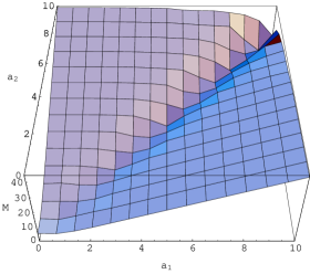
Figure 3.1: The unnormalized values of the $0^{++}$ glueball mass (the lowest eigenvalues of Eq. (3.39)) as a function of the two angular momenta. Note that this function is smooth everywhere except in the region $a_{1}=a_{2}\rightarrow\infty$.

                                                                                                                     

Figure 3.2: The ratio of the $0^{++*}$ mass to the $0^{++}$ mass along a generic direction, chosen here to be $a_{1}=2a_{2}=a$. Note, that the change in the ratio is tiny, and the asymptotic value of the ratio is the same as in Ref. [8] in the case of $a_{1}\rightarrow\infty$, $a_{2}=0$.

                                                                                                                     

Figure 3.3: The behavior of the ratio $r$ of the mass of the excited $0^{++*}$ glueball mass to the $0^{++}$ mass along the line $a_{1}=a_{2}$. Note, that along this direction the solutions behave very differently than anywhere else in the parameter space and depart significantly from the lattice results.

$$\begin{array}[]{|l|c|c|c|}\hline\cr\mbox{state}&\mbox{lattice}&\mbox{numerical}&WKB\\ \hline\cr 0^{++}&1.61\pm 0.15&1.61\;\mbox{(input)}&1.55\\ \hline\cr 0^{++*}&2.8&2.57&2.53\\ \hline\cr 0^{++**}&-&3.49&3.46\\ \hline\cr 0^{++***}&-&4.40&4.37\\ \hline\cr 0^{++****}&-&5.30&5.28\\ \hline\cr 0^{++*****}&-&6.20&6.18\\ \hline\cr\end{array}$$

Table 3.1: The masses of the first few $0^{++}$ glueballs in GeV. The first column gives the available lattice results [18, 19, 20], the second the asymptotic value of the supergravity calculation using the numerical method (the point is chosen to be $a_{1}=2a_{2}=20u_{0}$), while the third column the WKB result for the same supergravity approximation.

3.2.2 Masses of the $0^{-+}$ glueballs

The differential equation for $0^{-+}$ glueballs can be written as

$${1\over u^{3}}\partial_{u}\big{[}{1\over u}(u^{4}-a^{4}_{1})(u^{4}-a^{4}_{2})\partial_{u}\chi_{\theta_{2}}(u)\big{]}=-M^{2}{(u^{4}-a^{4}_{1})(u^{4}-a^{4}_{2})\over(u^{4}-a^{4}_{1})(u^{4}-a^{4}_{2})-u_{0}^{6}u^{2}}\ \chi_{\theta_{2}}(u)\ .$$ (3.40)

The corresponding mass spectrum can be obtained using a similar numerical method as for the $0^{++}$ glueballs. The dependence of the lightest $0^{-+}$ glueball mass on the angular momentum along a generic direction (chosen again to be $a_{1}=2a_{2}$) is given in Fig. 3.4. One can see that while the masses are fairly stable against variations of the angular momentum, just like in the case of $a_{2}=0$ discussed in [8], the actual values of the mass ratios compared to $0^{++}$ increase by a sizeable ($\sim 25\%$) value. The change is in the right direction as suggested by recent improved lattice simulations [20]. The actual asymptotic value of the mass ratio $\frac{m_{0^{-+}}}{m_{0^{++}}}=1.59$ is the same as for the $a_{2}=0$ case everywhere except very close to the region $a_{1}=a_{2}\gg u_{0}$. Table 3.2 contains the comparison of the lattice results to the supergravity results evaluated using the numerical and the WKB methods.

Just as for the case of the $0^{++}$ glueballs, this ratio behaves very differently along the special $a_{1}=a_{2}$ direction, and departs significantly from the lattice result $(\frac{m_{0^{-+}}}{m_{0^{++}}})_{lattice}=1.46$ as it can be seen in Fig. 3.5.

                                                                                                                     

Figure 3.4: The ratio of the lowest $0^{-+}$ mass to the lowest $0^{++}$ mass along a generic direction, chosen here to be $a_{1}=2a_{2}=a$. Note, that the ratio is very stable against the variations of the parameters. The actual change in the ratio is sizeable, and independent of the direction chosen in the $(a_{1},a_{2})$ parameter space (except the line $a_{1}=a_{2}$) and agrees with the ratio found in Ref. [8] for the case of $a_{1}\rightarrow\infty$, $a_{2}=0$. As explained in the text, this figure is only reliable for the regions $a\ll u_{0}$ and $a\gg u_{0}$ which are shown by solid lines, while for the intermediate region denoted by a dashed line there are corrections due to the non-vanishing off-diagonal components of the metric.

                                                                                                                     

Figure 3.5: The behavior of the ratio $r$ of the mass of the lowest $0^{-+}$ glueball mass to the lowest $0^{++}$ mass along the line $a_{1}=a_{2}$. As explained in the text, this figure is only reliable for the regions $a\ll u_{0}$ and $a\gg u_{0}$ which are shown by solid lines.

$$\begin{array}[]{|l|c|c|c|c|}\hline\cr\mbox{state}&\mbox{lattice}&\mbox{Num.}(a_{1,2}=0)&\mbox{Num.}(a_{1}=2a_{2}=20)&\mbox{WKB}\\ \hline\cr 0^{-+}&2.59\pm 0.13&2.00&2.57&2.53\\ \hline\cr 0^{-+*}&3.64\pm 0.18&2.98&3.49&3.46\\ \hline\cr 0^{-+**}&-&3.91&4.40&4.37\\ \hline\cr 0^{-+***}&-&4.83&5.30&5.28\\ \hline\cr 0^{-+****}&-&5.74&6.20&6.18\\ \hline\cr 0^{-+*****}&-&6.64&7.10&7.09\\ \hline\cr\end{array}$$

Table 3.2: The masses of the first few $0^{-+}$ glueballs in GeV. Unlike $0^{++}$ glueballs, the supergravity masses for these glueballs are sensitive to the values of $a_{1},a_{2}$. Two cases are displayed, illustrating the typical values that one gets for small and large $a_{1},a_{2}$ (the asymptotic values for large $a_{1},a_{2}$ are the same for any generic direction, i.e. with $a_{1}\neq a_{2}$). The lattice results are from [19, 20].

3.2.3 Masses of the KK modes of $S^{4}$

In terms of $u=\sqrt{\rho}$, equation (3.28) for the first KK doublet (3.5) reads

$$\partial_{u}\left[\frac{1}{u}\left((u^{4}-a_{1}^{4})(u^{4}-a_{2}^{4})-u^{2}u_{0}^{6}\right)\partial_{u}f(u)\right]-u^{3}\left(k^{2}+{4u^{2}\over h_{0}}H(u)\right)f(u)=0.$$ (3.41)

where

$$h_{0}(u)=\big{(}1-{a_{1}^{4}\over u^{4}}\big{)}\big{(}1-{a_{2}^{4}\over u^{4}}\big{)}-{u_{0}^{6}\over u^{6}}\ ,$$ (3.42)

$$H(u)=4h_{0}(u)\ \big{(}1-{a_{2}^{4}\over 2u^{4}}\big{)}+{a_{1}^{4}\over u^{4}}\big{(}1-{a_{2}^{4}\over u^{4}}\big{)}^{2}\ .$$ (3.43)

The components of the second doublet (3.6) give the same equation with $a_{1}$ and $a_{2}$ interchanged. Finally, the equation that determines the mass spectrum of the singlet (3.7) is

$$u^{2}\partial_{u}\left[\frac{1}{u}\left((u^{4}-a_{1}^{4})(u^{4}-a_{2}^{4})-u^{2}\right)f^{\prime}(u)\right]+u^{3}(8a_{1}^{4}+8a_{2}^{4}-k^{2}u^{2}-16u^{4})f(u)=0.$$ (3.44)

This is symmetric under the interchange of $a_{1}$ and $a_{2}$. One can again numerically determine the solutions of these equations using the shooting method. In Figs. 3.6 and 3.7 we show the behavior of the $SO(2)\times SO(2)$ singlet mode first along a generic direction (which was again chosen to be $a_{1}=2a_{2}$), and then along the special direction $a_{1}=a_{2}$. One can see that this mode does not decouple on any region of the parameter space. Figs. 3.8 and 3.9 show the similar plots for the non-singlet KK modes (for (3.41)), which similarly do not decouple anywhere in the parameter space. Tables 3.3 and 3.4 show the comparison of the first few KK modes evaluated using the numerical and the WKB methods.

                                                                                                                     

Figure 3.6: The mass ratio $r$ of the $SO(2)\times SO(2)$ singlet KK mode to the lowest $0^{++}$ glueball along the generic direction $a_{1}=2a_{2}$.

                                                                                                                     

Figure 3.7: The mass ratio $r$ of the $SO(2)\times SO(2)$ singlet KK mode to the lowest glueball mass $0^{++}$ along the special direction $a_{1}=a_{2}$.

$$\begin{array}[]{|l|c|c|}\hline\cr\mbox{state}&\mbox{numerical}&WKB\\ \hline\cr KK&2.15&2.00\\ \hline\cr KK^{*}&3.23&3.09\\ \hline\cr KK^{**}&4.20&4.09\\ \hline\cr KK^{***}&5.15&5.05\\ \hline\cr KK^{****}&6.07&5.99\\ \hline\cr KK^{*****}&6.99&6.91\\ \hline\cr\end{array}$$

Table 3.3: The masses of the first few singlet KK modes in GeV. The first column gives the asymptotic value of the supergravity calculation using the numerical method (the point is chosen to be $a_{1}=2a_{2}=20u_{0}$), while the second column the WKB result for the same supergravity approximation.

                                                                                                                     

Figure 3.8: The mass ratio $r$ of the $SO(2)\times SO(2)$ doublet KK mode to the lowest glueball masses along the generic direction $a_{1}=2a_{2}$.

                                                                                                                     

Figure 3.9: The mass ratio $r$ of the lightest glueball to the $SO(2)\times SO(2)$ doublet KK modes along the special direction $a_{1}=a_{2}$.

$$\begin{array}[]{|l|c|c|}\hline\cr\mbox{state}&\mbox{numerical}&WKB\\ \hline\cr KK&2.84&2.19\\ \hline\cr KK^{*}&3.80&3.34\\ \hline\cr KK^{**}&4.73&4.37\\ \hline\cr KK^{***}&5.54&5.36\\ \hline\cr KK^{****}&6.57&6.31\\ \hline\cr KK^{*****}&7.47&7.25\\ \hline\cr\end{array}$$

Table 3.4: The masses of the first few non-singlet KK modes in GeV. The first column gives the asymptotic value of the supergravity calculation using the numerical method (the point is chosen to be $a_{1}=2a_{2}=20u_{0}$), while the second column the WKB result for the same supergravity approximation.

3.2.4 Masses of the KK modes on the circle

Next we consider the KK modes coming from the compact D-brane coordinate. These modes have the form (3.4), where $\phi(u)$ obeys the differential equation

$$\partial_{u}\left[\frac{1}{u}\left((u^{4}-a_{1}^{4})(u^{4}-a_{2}^{4})-u^{2}\right)\partial_{u}\phi(u)\right]=\phi(u)u^{3}\bigg{(}k^{2}+\frac{9n^{2}(a_{1}^{4}-u^{4})(a_{2}^{4}-u^{4})}{A^{2}(u^{8}-u^{4}(a_{1}^{4}+a_{2}^{4})-u^{2}+a_{1}^{4}a_{2}^{4})}\bigg{)}\ .$$

One can again numerically solve these equations. For a generic direction (chosen to be again $a_{1}=2a_{2}$) we find that these modes decouple very quickly from the spectrum, just like in the case with one angular momentum parameter discussed in Ref. [8]. This is illustrated in Fig. 3.10. For the case of the special direction $a_{1}=a_{2}$, the numerical analysis of the decoupling is inconclusive. The masses of these KK modes grow much slower than for the generic case. At the point when our numerical solutions become unreliable, these modes are not decoupled yet, however one can not rule out the possibility that for $a\to\infty$ they eventually do decouple (see Fig. 3.11).

                                                                                                                     

Figure 3.10: The mass ratio $r$ of the lightest glueball to the KK mode on the compact D-brane coordinate $\theta_{2}$ along the generic direction $a_{1}=2a_{2}=a$. Just as for the case with only one angular momentum, these states decouple very quickly from the spectrum.

                                                                                                                     

Figure 3.11: The mass ratio $r$ of the lightest glueball to the KK mode on the compact D-brane coordinate $\theta_{2}$ along the special direction $a_{1}=a_{2}$.

$$\begin{array}[]{|l|c|c|}\hline\cr\mbox{state}&\mbox{numerical}&WKB\\ \hline\cr KK&11.27&11.24\\ \hline\cr KK^{*}&11.48&11.45\\ \hline\cr KK^{**}&11.76&11.72\\ \hline\cr KK^{***}&12.09&12.06\\ \hline\cr KK^{****}&12.48&12.45\\ \hline\cr KK^{*****}&12.92&12.89\\ \hline\cr\end{array}$$

Table 3.5: The masses of the first few KK modes on the circle in GeV. Along a generic direction these KK modes decouple, thus we have chosen an arbitrary point $a_{1}=2a_{2}=2.5u_{0}$ for the comparison of the numerical and WKB results. which are given in the first and second column.

4 Conclusions

In this paper we have presented a two-parameter family of supergravity models of non-supersymmetric $3+1$ dimensional $SU(N)$ Yang–Mills theory, based on regular geometries with D4-brane charge. In these models, we have evaluated the mass spectra of the scalar glueballs and some of the related KK modes everywhere on the two dimensional parameter space using both numerical and analytic (WKB) methods. We find that the glueball mass ratios are very stable against the variation of the angular momentum parameters. The asymptotic values of these ratios for large angular momenta are in good agreement with the most recent lattice results everywhere in the parameter space except along a special line $a_{1}=a_{2}\gg u_{0}$ (which is exactly the region where the WKB approximation breaks down, and also the region where the inner and outer horizons approach each other and the supergravity approximation approaches a discontinuous limit). The KK modes on the compact D-brane coordinate decouple for large angular momenta everywhere (except perhaps along $a_{1}=a_{2}$, where our analysis of decoupling is inconclusive). The KK modes on the $S^{4}$ however do not decouple from the spectrum anywhere in the parameter space in the supergravity approximation used in this paper.

The masses evaluated in this paper in the supergravity approximation can in principle get large corrections when extrapolating from the strong coupling (large $\lambda$) regime to the weak-coupling regime of the Yang–Mills theory. If the spectrum of the corresponding string models at small $\lambda$ do indeed reproduce the Yang–Mills spectrum, a natural question to ask is why the glueball masses (or perhaps only the glueball mass ratios) would get small corrections, while the KK masses get large corrections. Since in the limit $a_{1},a_{2}\gg u_{0}$ the metric approaches the supersymmetric space (2.31), it is possible that a subset of the masses may be protected by supersymmetry (as explained in Sec. 2.3, the naive limit $u_{0}\to 0$ does not lead to a supersymmetric theory, since it does not have fermions in the spectrum). A problem of interest is thus to investigate the supersymmetric model with $u_{0}=0$, and determine which scalars belong to short BPS multiplets, and which ones are in long multiplets. Since the masses of the scalars belonging to short multiplets should not be changed in the $\lambda\ll 1$ regime, this could explain why the $0^{-+}$ glueball masses are so close to the lattice values, and it may be used as a highly non-trivial quantitative test of the conjectured relation of supergravity to non-supersymmetric $SU(N)$ Yang–Mills theory.

References

• [1] J. M. Maldacena, “The Large $N$ Limit of Superconformal Field Theories and Supergravity”, Adv. Theor. Math. Phys. 2 (1998) 231, hep-th/9711200; S. S. Gubser, I. R. Klebanov, and A. M. Polyakov, “Gauge theory correlators from noncritical string theory,” Phys. Lett. B428 (1998) 105, hep-th/9802109; E. Witten, “Anti-de Sitter space and holography,”, Adv. Theor. Math. Phys. 2 (1998) 253, hep-th/9802150.
• [2] E. Witten, “Anti-de Sitter space, thermal phase transition, and confinement in gauge theories”, Adv. Theor. Math. Phys. 2 (1998), hep-th/9803131.
• [3] D. J. Gross and H. Ooguri, “Aspects of large-$N$ gauge theory dynamics as seen by string theory”, Phys. Rev. D58 (1998) 106002, hep-th/9805129.
• [4] C. Csáki, H. Ooguri, Y. Oz, and J. Terning, “Glueball mass spectrum from supergravity”, hep-th/9806021.
• [5] R. de Mello Koch, A. Jevicki, M. Mihailescu and J. Nunes, “Evaluation of glueball masses from supergravity”, Phys. Rev. D58 (1998) 105009, hep-th/9806125; M. Zyskin, “A note on the glueball mass spectrum”, Phys. Lett. B439 (1998) 373, hep-th/9806128.
• [6] J.G. Russo, “New compactifications of supergravities and large $N$ QCD”, hep-th/9808117.
• [7] A.  Hashimoto and Y. Oz, “Aspects of QCD dynamics from string theory”, hep-th/9809106.
• [8] C. Csáki, Y. Oz, J. Russo and J. Terning, “Large $N$ QCD from rotating branes”, hep-th/9810186.
• [9] J.A. Minahan, “Glueball Mass Spectra and Other Issues for Supergravity Duals of QCD Models”, hep-th/9811156.
• [10] J.G. Russo and K. Sfetsos, “Rotating D3 branes and QCD in three dimensions”, hep-th/9901056.
• [11] H. Ooguri, H. Robins and J. Tannenhauser, “Glueballs and Their Kaluza–Klein Cousins”, Phys. Lett. B437 (1998) 77, hep-th/9806171.
• [12] S.S. Gubser, “Thermodynamics of spinning D3-branes”, hep-th/9810225.
• [13] P. Kraus, F. Larsen and S.P. Trivedi, “ The Coulomb Branch of Gauge Theory from Rotating Branes”, hep-th/9811120.
• [14] R.G. Cai and K.S. Soh, “Critical behavior in the rotating D-branes”, hep-th/9812121.
• [15] M. Cvetič and D. Youm, “Rotating intersecting M-branes”, Nucl. Phys. B499 (1997) 253, hep-th/9612229.
• [16] K. Sfetsos, “Branes for Higgs phases and exact conformal field theories”, hep-th/9811156.
• [17] E. Witten, Phys. Rev. Lett. 81 (1998) 2862, hep-th/9807109.
• [18] M. J. Teper, “Physics from the lattice: Glueballs in QCD: Topology: $SU(N)$ for all $N$,” hep-lat/9711011.
• [19] C. Morningstar and M. Peardon, “Efficient glueball simulations on anisotropic lattices,” Phys. Rev. D56 (1997) 4043, hep-lat/9704011.
• [20] M.Peardon, “Coarse lattice results for glueballs and hybrids,” Nucl.Phys. B (Proc.Suppl.) 63, 22 (1998), hep-lat/9710029; C. Morningstar and M. Peardon, “The glueball spectrum from an anisotropic lattice study,” hep-lat/9901004.