CERN-TH/98-375

OUTP-98-81-P

SPIN-98-7

hep-th/9902058

String Thermodynamics in D-Brane Backgrounds

S.A. Abel^a,, J.L.F. Barbón^b,, I.I. Kogan^c,, E. Rabinovici^d,

$a$ Theory Division, CERN, CH-1211 Geneva 23, Switzerland
$b$ Spinoza Institute, Leuvenlaan 4, 3584 CE, Utrecht, The Netherlands
$c$ Theoretical Physics, 1 Keble Road, Oxford OX1 3NP, UK
$d$ Racah Institute of Physics, The Hebrew University, Jerusalem, Israel

Abstract

We discuss the thermal properties of string gases propagating in various D-brane backgrounds in the weak-coupling limit, and at temperatures close to the Hagedorn temperature. We determine, in the canonical ensemble, whether the Hagedorn temperature is limiting or non-limiting. This depends on the dimensionality of the D-brane, and the size of the compact dimensions. We find that in many cases the non-limiting behaviour manifest in the canonical ensemble is modified to a limiting behaviour in the microcanonical ensemble and show that, when there are different systems in thermal contact, the energy flows into open strings on the ‘limiting’ D-branes of largest dimensionality. Such energy densities may eventually exceed the D-brane intrinsic tension. We discuss possible implications of this for the survival of D$p$-branes with large values of $p$ in an early cosmological Hagedorn regime. We also discuss the general phase diagram of the interacting theory, as implied by the holographic and black-hole/string correspondence principles.

CERN-TH/98-375

1 Introduction and Background

Models in which the particle spectrum has the Hagedorn form [1],

$$\rho(m)\sim m^{a}\,\,e^{bm}$$ (1)

are of great interest because of their thermodynamic properties. For example, for $a<-5/2$ (in four dimensions) and, at sufficient energy density, a system like this has a negative specific heat. Thermodynamic quantities are not extensive and two such sytems cannot establish an equilibrium [2].

This type of spectrum first arose in the context of statistical bootstrap models [1, 3] and, for hadrons, such behaviour indicates that they are composed of more fundamental constituents [4]. In fundamental string theories we find the same kind of spectrum [5, 6, 7, 8], and a search for hints to the existence of ‘string constituents’ is of great interest.

On a more practical level, regimes of Hagedorn behaviour of weakly-coupled strings are interesting in the context of stringy cosmological models [7]. In particular, there has been much work recently in models where the string scale can be significantly lower than the Planck scale [9], perhaps even as low as the  TeV scale [11, 12]. These models involve string theory in backgrounds in which the gauge sector is confined to extended topological defects (branes) of various kinds. Particularly tractable are models constructed with Dirichlet $p$-branes [13]. The visible universe could, for example, correspond to a D3-brane, and the cosmological behaviour of such systems is only beginning to be studied  [11, 12, 14].

In this paper we study various aspects of the thermodynamics of fundamental strings in backgrounds with webs of intersecting D-branes. For any particular brane structure (i.e. number and spatial arrangement of the D-branes), there are open strings in different sectors, labeled by the D-brane sets to which they are attached, as well as closed strings propagating in the bulk. We determine the thermodynamic properties of the different D-brane sectors at energy densities larger than the fundamental string scale, to leading order in string perturbation theory, and paying special attention to the dependence on the various T-moduli (volumes). For early work on various aspects of Hagedorn behaviour with D-branes see for example [15, 16, 17, 18, 19].

One particularly interesting fact is that for ordinary ten-dimensional superstrings (including the heterotic) the closed-string sector has a Hagedorn temperature which is ‘non-limiting’ (in that it requires a finite amount of energy to reach it, in the description provided by the canonical ensemble), whilst Type–I open strings have a ‘limiting’ Hagedorn temperature [5, 12]. It was pointed out recently in Ref. [19] that open-string sectors in D$p$-branes show ‘limiting’ behaviour provided $p\geq 5$. On the other hand, for $p<5$, open strings seem to show ‘non-limiting’ behaviour, similar to that of closed strings. It should be noted that different sectors have the same Hagedorn temperature in perturbation theory, since the critical behaviour can be related to the onset of infrared divergences due to a closed-string state becoming massless at the Hagedorn temperature [20, 21]. Provided this ‘tachyonic’ closed-string state couples to all D-branes, all the topologically distinct open-string sectors will share the same critical temperature.

We begin our discussion in section 2 by calculating the canonical (single-string) density of states of an open string propagating in various D-brane backgrounds. In particular we generalize the analysis to the case where the dimensions are large but compact and pay special attention to whether the Hagedorn temperature appears to be ‘limiting’ or ‘non-limiting’. When dealing with finite and large dimensions, the experience with closed strings (c.f. [8]) tells us that the thermodynamic properties ought to change as the energy is raised through ‘thresholds’. These thresholds correspond to the string being able to ‘feel’ extra dimensions by producing winding or heavy momentum modes and we shall find that this is indeed the case with open strings. Any dependence on the finite size of extra dimensions is of particular interest because phenomenologically viable D-brane scenarios typically require large compact dimensions in order to explain why the weak scale is so much lower than the Planck scale.

In section 3 we derive the thermodynamic properties in the microcanonical ensemble. As with closed strings, this analysis is required once the canonical ensemble exhibits esoteric features such as supposedly negative specific heat, and leads to a better understanding of the thermodynamic properties. The more limited information encoded in the free energy (the canonical ensemble) concerning the properties of non-limiting strings is greatly enhanced by studying the microcanonical ensemble.

Most importantly the universal presence of gravity in any string system means that the infinite volume limit (the thermodynamic limit) at finite energy density does not exist in a strict sense, due to the Jeans instability [22, 21], and the holographic bound [23]. Thus, consistency requires working in finite volume, and investigating whether there are regimes of approximate thermodynamic behaviour for each individual case.

To do this, we shall work in the simplest finite-volume backgrounds, i.e. toroidal compactifications. For closed strings in the ideal-gas approximation, it was found in [7, 8] that winding modes tend to work in favour of positive specific heat. Indeed, if winding modes carry a sizeable proportion of the energy, a superficially non-limiting behaviour according to the canonical ensemble may turn into a limiting behaviour in the true microcanonical analysis.

We find many examples of this phenomenon in the brane backgrounds. As the microcanonical discussion can be rather technical, it is worth previewing the resulting physical picture. Imagine heating up open-string excitations on a thermally isolated D-brane wrapped on a finite-volume torus. Consider a D$p$-brane for which the canonical ensemble predicts a non-limiting behaviour. Eventually the critical Hagedorn energy density is reached on the brane and open strings begin looping into the bulk volume although their ends must stay attached to the brane. The D-brane is now surrounded by an open-string cloud which spreads as we raise the temperature. At some point a few energetic strings emerge and, as we raise the temperature still further, the spectrum of a canonically non-limiting open-string system becomes resolved into a peak of low-energy excitations and a few energetic excitations which carry most of the energy. Eventually these modes are able to wind in the Dirichlet directions and their number grows rapidly once they start winding. The thermal properties begin to resemble those of the system in a small, totally compact volume. As we approach the Hagedorn temperature, the specific heat increases dramatically, and we find that we cannot supply enough energy to raise the temperature to the Hagedorn temperature. The limiting behaviour has been restored.

In the more general multibrane configurations there are several types of open strings depending on how these strings stretch between branes attached at their end-points. We calculate the entropy for each such class. We find that the critical behaviour is very similar in all open-string sectors.

The thermal interaction of two or more Hagedorn systems then follows directly (in section 4) from the microcanonical discussion and turns out to be quite unusual. In particular, we will show that systems which are ‘non-limiting’ tend to give their energy up to ‘limiting’ systems. Thus if we take our previously isolated D-brane and place it in a bath of closed strings, the energy of the former increases in the manner described above, almost without limit. This curious and possibly violent disequilibrium is due to differently diverging specific heats and is reminiscent of systems with negative specific heat (although we stress that most specific heats are found to be positive below the Hagedorn temperature).

We then speculate on how such a process might end. We suggest that eventually the energy density of the open-string gas becomes greater than the D-brane tension. At this point the system is unstable towards the thermal nucleation of D-brane–antiD-brane pairs of various dimensions and topological structures. We make some estimates of the production rate under the assumption that the brane–antibrane pairs form a dilute plasma.

Finally, in section 5, we suggest a phase diagram including the effects of string interactions. Most notably, we use the correspondence principle of [24] to derive high-energy generalizations of previously studied phase diagrams in the context of the SYM/AdS correspondence [25, 26, 19, 36]. It is suggested that, at weak string coupling, the Hagedorn regime is always bounded by a black-hole-dominated phase, which subsequently saturates the holographic bound [23]. Indeed, black holes seem to emerge quite often when the Hagedorn regime is probed [6, 27, 28, 24, 19].

2 The Canonical Ensemble in the Presence of D-branes

We shall consider models of Type–II strings on tori, with a number of D-branes wrapped in a possibly complicated intersection pattern, together with orientifold planes ensuring the appropriate cancellation of tadpoles and anomalies.

In addition to the closed strings propagating in the bulk, we have different sectors of open strings, defined by the classes of branes to which they are attached. A given class of open strings will be labeled $(p,q)$ if they connect a D$p$-brane and a D$q$-brane. The relative orientation of the branes is in principle arbitrary, although we will only consider supersymmetric intersections, i.e. those for which the $(p,q)$ strings propagating along the intersection submanifold have a supersymmetric ground state.

Each $(p,q)$ system is characterized by a different partition of the 10 space-time dimensions into Neumann–Neumann (NN), Dirichlet–Dirichlet (DD), or mixed (Dirichlet–Neumann (DN) plus Neumann–Dirichlet (ND)):

$$10=d_{NN}+d_{DD}+d_{ND}+d_{DN},$$ (2)

where $d_{ND}+d_{NN}=p+1$ and $d_{DN}+d_{NN}=q+1$. Accordingly, we denote the radii of the torus in these directions by $R_{NN},R_{DD},R_{ND}$ and $R_{DN}$ (some of which could be infinite). Notice that this labeling of the torus radii depends on the particular $(p,q)$ system of open strings we focus on.

The total number of directions with mixed boundary conditions for a given $(p,q)$ system is denoted by

$$\nu\equiv d_{ND}+d_{DN},$$ (3)

and for a supersymmetric intersection it must take values

$$\nu=0\,({\rm mod}\;4).$$ (4)

The simplest case of $\nu=0$ corresponds to parallel branes. Intersections with $\nu=4$ are all D$p$–D$(p+4)$ systems and their T-duals. Finally, a prototype of $\nu=8$ system is the D0–D8 intersection and all T-duals. So, for example a Type–I model with wrapped D5- and D1-branes contains closed strings and open strings in all $\nu=0,4,8$ sectors.

We always assume that the system is at weak coupling so that the mass of the D-branes is large and perturbation theory around the D-brane background is a good approximation. In particular in this limit we can neglect brane creation in the vacuum and can neglect the effects of perturbations of the brane itself on the thermodynamics. In later sections we discuss the meaning of this assumption in more detail, and in particular the thermodynamic systems in which it might be expected to break down.

One additional point. For calculations in purely perturbative closed-string theories, an important question was whether to take winding number and momentum to be conserved in the compact dimensions. Indeed, the thermodynamic properties are typically found to be qualitatively different if these quantum numbers are conserved. In this paper we are ultimately interested in the thermodynamic properties of two or more systems in equilibrium in a D-brane background. Hence in all of our calculations we do not conserve winding number or momentum in the compact dimensions, since for example D-branes can absorb and emit momentum, and winding number can be transferred from a gas of open strings on the brane to a gas a closed strings in the bulk.

2.1 Single-String Density of States

The open strings in the $(p,q)$ sector have NN momenta, DD windings, and oscillators in all transverse directions. Notice that they do not have momentum or winding quantum numbers in the ND or DN directions. As a result, the thermodynamic quantities of the $(p,q)$ system are independent of the ND, DN moduli $R_{ND},R_{DN}$. Using T-duality, we assume that all radii are larger or equal than the T-selfdual radius: $R_{NN},R_{ND},R_{DN},R_{DD}\geq 1$ in string units. In fact, when the radii are of stringy size, the NN or DD character is not sharply defined, but then we shall see that thermodynamics depends only on $\nu$ as a dimensional parameter, which is T-duality invariant.

The single-string energy is given by

$$\varepsilon^{2}=({\vec{p}}\,)^{2}+\left({\rm Osc}_{\sigma}-a_{\sigma}\right).$$ (5)

The constant $a_{\sigma}$ is the normal ordering intercept with the spin structure $\sigma$: $a=1$ for bosonic strings, $a_{\rm NS}=1/2$ for Neveu–Schwarz spin structure and $a_{\rm R}=0$ for the Ramond sector, in the case of superstrings. Open strings on D-branes have $a_{\rm R}=0$ and $a_{\rm NS}=(\nu-4)/8$. Here ${\vec{p}}$ is the momentum in the spatial NN directions plus the contributions from the open-string windings in the DD directions,

$$({\vec{p}}\,)^{2}=\sum_{i\in NN}\frac{n_{i}^{2}}{R_{i}^{2}}+\sum_{i\in DD}l_{i}^{2}R_{i}^{2},$$ (6)

where $R_{i}$ are the torus radii. The oscillator part ${\rm Osc}_{\sigma}$ receives integer contributions from world-sheet bosons in NN or DD directions, but half-integer contributions from the bosons in ND and DN directions. World-sheet fermions contribute according to the spin structure (which is correlated with the bosonic modding, i.e. fermions have the same modding as bosons in the R sector, and opposite in the NS sector).

The number of states with a particular value of the oscillator level, ${\rm Osc}=n$, is obtained from

$$d(n)=\frac{1}{2\pi i}\oint{\mbox{d}q\over q^{n+1}}\;f(q),$$ (7)

with the function

$$f(q)=\mbox{Tr}_{\rm osc}\,q^{\rm Osc}$$ (8)

denoting the oscillator trace generating function. In a manifestly supersymmetric treatment, such as the Green-Schwarz formalism, the modding of fermionic and bosonic oscillators must be the same: integer in NN+DD directions and half-integer in ND+DN directions. Thus, we get a factor of

$$\prod_{m=0}^{\infty}\left({1+q^{m}\over 1-q^{m}}\right)$$ (9)

for each of the $8-\nu$ transverse NN+DD directions, and a factor of

$$\prod_{m=0}^{\infty}\left({1+q^{m+\frac{1}{2}}\over 1-q^{m+\frac{1}{2}}}\right)$$ (10)

for each of the $\nu$ directions with ND or DN boundary conditions. In addition, we have the degeneracy from fermionic zero modes, which can be determined from the size of the corresponding massless multiplets. It is given by $C_{\nu}=2^{4-\nu/2}$, i.e. a ten-dimensional vector multiplet $(C_{0}=16)$ for $\nu=0$, a half-hypermultiplet $(C_{4}=4)$ for $\nu=4$, and a single state for $\nu=8$. These degeneracies may be affected by ‘flavour’ factors, such as a factor of $N^{2}$ for $N$ parallel D-branes in $\nu=0$, a factor of $2$ for both orientations (i.e. $(p,q)$ and $(q,p)$ strings) in $\nu\neq 0$ sectors, or factors of $1/2$ due to orientifold projections.

Putting all factors together, and using Jacobi’s and Dedekind’s functions, we find, for each single orientation and flavour sector:

$$f(q)=\left({\theta_{2}(q)\over\eta(q)^{3}}\right)^{4-{\nu\over 2}}\,\left({\theta_{3}(q)\over\theta_{4}(q)}\right)^{\nu\over 2}.$$ (11)

A crucial property of (11) is that the contribution from ND and DN directions has no modular anomaly under modular transformations, consistent with the absence of zero modes in those directions.

Using the modular properties of $f(q)$ the integrand of (7) can be approximated for $q\rightarrow 1$ [29]. If we define $q=1-\xi$ then

$$\frac{f(q)}{q^{n+1}}\sim\left(\frac{\xi}{2\pi}\right)^{4-\nu/2}\,\exp\left(2\pi^{2}/\xi+(n+1)\xi\right).$$ (12)

There is a saddle point at $\xi_{0}=\sqrt{2}\pi/\sqrt{n+1}$. Upon expanding about this and doing the Gaussian integral which results, one finds that the following level-density, a generalization of results in [5, 6, 8],

$$d(n,n_{i},l_{i})\sim n^{(\nu-11)/4}\;e^{\beta_{c}\sqrt{n}},$$ (13)

where $\beta_{c}=2\sqrt{2}\pi$. The level density tells us the number of oscillator modes in a given momentum and winding sector. The single-string density of states is then obtained by summing over all zero-mode quantum numbers, with the constraint of Eq. (5)

$$\omega(\varepsilon)\mbox{d}\varepsilon\sim\sum_{l_{i},n_{i}}\varepsilon^{(\nu-9)/2}e^{\beta_{c}\sqrt{n(\varepsilon)}}\;\mbox{d}\varepsilon,$$ (14)

with the function $n(\varepsilon)$ defined by (5) upon setting ${\rm Osc}=n(\varepsilon)$. Note that, since all dimensions are taken to be compact, there are no integrations over continuous momenta and no volume factors. These are recovered once we let the dimensions become large and perform a large-$\varepsilon$ expansion of $n(\varepsilon)$;

$$\sqrt{n(\varepsilon)}=\varepsilon-\sum_{i\in NN}\frac{n_{i}^{2}}{2\,\varepsilon\,R_{i}^{2}}-\sum_{i\in DD}\frac{l_{i}^{2}R_{i}^{2}}{2\,\varepsilon}+\ldots$$ (15)

The summations over $n_{i}$ and $l_{i}$ can be approximated by Gaussian integrals when each successive term in Eq. (15) is small and the summations are nearly continuous, which requires

$$R_{NN}^{2} \gg 1/\varepsilon$$

$$R_{DD}^{2} \ll \varepsilon\,.$$ (16)

The first condition is always satisfied (by assumption, since we have T-dualized the small directions and since $\varepsilon\gg 1$ for the asymptotic approximation (14) to be accurate at all). The second condition gives a threshold energy, above which the string is energetic enough to wind around Dirichlet directions which we shall define (for later convenience) as,

$$\varepsilon_{0}=2R^{2}_{DD}/\beta_{c}.$$ (17)

When $\varepsilon\ll\varepsilon_{0}$ the Dirichlet directions can only contribute when $l_{i}$ is zero. The single-string density of states in the limits of high and low energy is

$$\omega(\varepsilon)\mbox{d}\varepsilon=\left\{\begin{array}[]{ll}\beta_{c}\;V_{NN}(\beta_{c}\,\varepsilon)^{-d_{DD}/2}\;e^{\beta_{c}\,\varepsilon}\;\mbox{d}\varepsilon&\varepsilon\ll\varepsilon_{0}\\ \\ f\;\beta_{c}\;e^{\beta_{c}\,\varepsilon}\;\mbox{d}\varepsilon&\varepsilon\gg\varepsilon_{0}.\end{array}\right.$$

where $V_{NN}$ is the volume of the spatial Neumann directions, and where we have defined the ratio of volumes as

$$f=\frac{V_{NN}}{V_{DD}}.$$ (18)

Note that the density of states changes as we go through the energy threshold and strings are able to wind in the Dirichlet direction. The exponent in Eq. (2.1) counts the number of DD directions in which strings are not able to wind and hence it can be generalized to the case where the Dirichlet directions have varying sizes; one instead finds a series of thresholds and an $\omega(\varepsilon)$ which interpolates between the two extremes in Eq. (2.1). To accomodate this possibility, we define an effective dimension for open strings $d_{o}(\varepsilon)$ which is the number of DD dimensions around which the strings cannot wind (i.e. which do not obey Eq. (2.1)),

$$0\leq d_{o}\leq d_{DD}.$$ (19)

We define the volume of these dimensions to be $V_{o}$ and then have

$$\omega({\varepsilon})=\beta_{c}\,f\;V_{o}\frac{e^{\beta_{c}\varepsilon}}{(\beta_{c}\,\varepsilon)^{\gamma_{o}+1}},$$ (20)

where the critical exponent $\gamma_{o}$ is given by

$$\gamma_{o}=\frac{d_{o}}{2}-1.$$ (21)

We can, at this point, also define an effective number of large space-time dimensions which is a function of $\varepsilon$,

$$D_{o}(\varepsilon)=d_{NN}+d_{o}(\varepsilon)\leq 10-\nu.$$ (22)

Notice that, in this definition, we have excluded possible ‘large’ ND+DN directions, as they play no role in opening thresholds.

Examples

For what is normally meant by a D$p$-brane (i.e. a $(p+1)$-dimensional world-volume with $9-p$ non-compact Dirichlet directions and $p$ spatial non-compact Neumann directions), we would recover $d_{NN}=p+1$ and always have $\varepsilon<\varepsilon_{0}=\infty$, and hence

$$\omega(\varepsilon)\,\mbox{d}\varepsilon=\beta_{c}\;V_{NN}\;(\beta_{c}\,\varepsilon)^{-(10-d_{NN})/2}\;e^{\beta_{c}\,\varepsilon}\,\mbox{d}\varepsilon=\beta_{c}\;V_{p}\;(\beta_{c}\,\varepsilon)^{(p-9)/2}\;e^{\beta_{c}\,\varepsilon}\mbox{d}\varepsilon,$$ (23)

in accord with Ref. [19]. However Eq. (20) carries useful additional information about what happens to the density of states as dimensions expand or contract. In particular we see a kind of behaviour that is familiar from closed-string thermodynamics. When a Dirichlet direction becomes sufficiently small or strings become sufficiently energetic (given by Eq. (2.1)), open strings are able to wind around it. This is reflected in the density of states by that dimension becoming ‘compact’; when all the Dirichlet directions are compact, and $\varepsilon\gg\varepsilon_{0}$ we instead find

$$\omega(\varepsilon)\,\mbox{d}\varepsilon=\beta_{c}\;\frac{V_{p}}{V_{D-p-1}}\;e^{\beta_{c}\,\varepsilon}\;\mbox{d}\varepsilon.$$ (24)

Open strings in Type–I theories propagate through the whole Neumann volume, and hence the calculation is the same as for open strings on the $(d_{NN}-1)$-brane in Type–II theory; if the space is non-compact we would again take $\varepsilon\ll\varepsilon_{0}$ in which case we recover the non-compact result of Ref. [12] when $\gamma_{o}=(D_{o}-d_{NN})/2-1=-1$. However when any of the dimensions are compact, there is an energy dependence in the density of states in this case as well. In particular, we could consider the case where there are 3+1 directions which are much larger than the string scale, $c$ compactified directions of order the string scale and $6-c$ compactified directions which are much smaller than the string scale. (After a duality transformation these become $6-c$ Dirichlet directions much larger than the string scale with heavy winding modes.) In this case the density of states depends on how many of the compact dimensions the strings are able to probe. That is, when the internal energy is very large the open strings are able to propagate throughout the whole space and we have $\gamma_{o}+1=0$. However, when $\varepsilon\ll\varepsilon_{0}$ we instead have $\gamma_{o}+1=d_{DD}/2=3-c/2$ (since in the T-dualized theory the very small Neumann directions have become Dirichlet directions with winding modes which are too heavy to excite). For cases of phenomenological interest there may be varying radii and hence a complicated energy dependence in $\gamma_{o}$.

Free Energy

The canonical free energy $F=-{1\over\beta}\,{\rm log}\,Z$ is now given by the Laplace transform of $\omega(\varepsilon)$. The different energy thresholds in (2.1) translate into analogous thresholds in temperature, since $\langle\varepsilon\rangle\sim(\beta-\beta_{c})^{-1}$, we can regard $V_{o}$ as the volume of the DD directions satisfying

$$1\gg{\beta-\beta_{c}\over\beta_{c}}\gg{1\over R_{DD}^{2}}.$$

In this region, we have the approximate behaviour

$${\rm log}\,Z \sim \int\mbox{d}\varepsilon\,\omega(\varepsilon)\,e^{-\beta\varepsilon}$$ (25)

$$= f\,V_{o}\,\left(\frac{\beta-\beta_{c}}{\beta_{c}}\right)^{{d_{o}\over 2}-1}.$$

Notice that, as soon as we assume compact dimensions, we require additional information about the system as a whole (i.e. its total energy) in order to calculate the free energy. When all dimensions are assumed to be non-compact from the outset this problem of course never arises since it would require an infinite amount of energy for a string to wind so that the above is always valid. However, the thermodynamic limit means taking an infinite volume and filling it with a finite energy density. Consequently, in a compact space of any size, there can in principle be enough energy available for strings to wind.

2.2 Euclidean Approach

This question of the effect of compact dimensions on the thermodynamic limit (which was just stated in rather simple minded terms) is of central importance and was addressed for closed strings in Ref. [8]. It will require a proper understanding of the microcanonical ensemble which will be the main goal of the next section. As a first step, let us recalculate the density of states using the method of Refs.  [15, 17, 19] in which the free energy is determined by compactifying in an imaginary time direction with periodicity $\beta$. The particular benefit of this method is that it identifies the leading and subleading contributions to the free energy as singularities of the partition function in the complex $\beta$ plane, as a result of ‘massless’ closed-string exchange between the branes. Our main task therefore is to find the structure of these singularities.

In the $(p,q)$ sector the free energy is a sum of terms for different spin structures $\{\sigma\}$, each one of the form

$${\rm log}\,Z_{(p,q,\sigma)}=\frac{1}{2}\int{dt\over t}\mbox{Tr}_{\rm open}\,\,\,{\cal O}_{\rm GSO}^{(\sigma)}\,\,\,e^{-t\Delta_{\rm open}},$$ (26)

where ${\cal O}_{\rm GSO}$ is (a piece of) the GSO projector, i.e. $\pm 1$ or $\pm(-1)^{F}$ depending on the particular spin structure. The open-string world-sheet hamiltonian is

$$\Delta_{\rm open}=4\pi^{2}n_{\sigma}^{2}/\beta^{2}+({\vec{n}}/R_{NN})^{2}+({\vec{l}}\,R_{DD})^{2}+({\rm Osc}-a)_{\sigma},$$ (27)

with $n_{\sigma}$ an integer or half-integer depending on the bosonic or fermionic statistics of the space-time states being traced over. For notational simplicity, we are assuming here equal radii within each NN or DD class of directions. The generalization to arbitrary radii is straightforward.

Upon Poisson resummation in $n_{\sigma}$, ${\vec{n}}$ and ${\vec{l}}$ we find

$${\rm log}\,Z_{(p,q,\sigma)} \sim \beta\cdot f\cdot\int{dt\over t}t^{-(d_{NN}+d_{DD})/2}\,\mbox{Tr}_{\rm osc}\,{\cal O}_{\rm GSO}^{(\sigma)}\,e^{-t({\rm Osc}-a)_{\sigma}}\times$$ (28)

$$\hskip 170.71652pt\sum_{n,{\vec{n}},{\vec{l}}}(-1)^{n{\bf F}_{\sigma}}\,e^{-{2\pi^{2}\over t}\Delta^{(0)}_{\rm closed}},$$

where $n$ is now an integer and ${\bf F}$ is the space-time fermion number. The zero-mode action now reads

$$2\;\Delta^{(0)}_{\rm closed}=({\vec{n}}\,R_{NN})^{2}+({\vec{l}}/R_{DD})^{2}+n^{2}\beta^{2}/4\pi^{2}.$$ (29)

This notation suggests that the appropriate modular transformation to the closed-string channel is given by the change of variables $t=2\pi^{2}/s$, which acts on the theta functions from the oscillator traces in the following universal form:

$$\mbox{Tr}_{\rm open\,\,osc}\,{\cal O}_{\rm GSO}^{(\sigma)}\,e^{-t({\rm Osc}-a)_{\sigma}}\sim s^{-4+\nu/2}\,\langle{\rm D}p_{\rm osc}|{\cal O}_{\rm GSO}^{(\sigma)}\,e^{-s({\rm Osc}_{L}+{\rm Osc}_{R}-a_{L}-a_{R})_{\sigma}}|{\rm D}q_{\rm osc}\rangle.$$ (30)

The power of $s^{-4+\nu/2}$ in this formula comes from the modular transformation of eight-dimensional transverse oscillator traces as in (11). The closed strings propagating between D-brane boundary states (as given for example in [30]) do not have windings and momenta at the same time in any direction, so that we can assume trivial level matching for all spin structures when evaluating Eq. (30):

$$({\rm Osc}-a)_{L}=({\rm Osc}-a)_{R}.$$ (31)

Now, putting everything together, one obtains an expression with the form of a closed-string propagator:

$${\rm log}\,Z\sim+f\int ds\,\sum_{\lambda}g_{\lambda}\,e^{-s\lambda},$$ (32)

where the quantities

$$2\,\lambda=n^{2}\beta^{2}/4\pi^{2}+({\vec{l}}/R_{DD})^{2}+({\vec{n}}\;R_{NN})^{2}+4\left({\rm Osc}-a\right)$$ (33)

are those eigenvalues of the full closed-string kernel, $\Delta_{\rm closed}$, with non-vanishing overlap with both D-brane states:

$$\langle\lambda|{\rm D}p,{\rm D}q\rangle\neq 0$$ (34)

and $g_{\lambda}$ denotes the multiplicity of a given eigenvalue. The spectrum is discrete at finite volume, which justifies writing the free energy as a discrete sum.

This result admits some simple generalizations. In the presence of orientifold planes, analogous considerations hold, replacing the D-brane boundary states by orientifold boundary states $|{\rm O}p\rangle$, and introducing the orientation projection in the open-string sector. The result is an expression of the same general form as Eq. (32), with a different modding of quantum numbers in the closed-string sector (see Ref. [17]). For example, a crosscap restricts the winding numbers to be even.

One can also generalize the previous formulas to the case where various D-branes and orientifold planes have some transverse separation $L_{DD}$. This simply introduces a stretching energy for the open strings of the form $L_{DD}/2\pi$, which translates into a new term in the closed-string channel expression Eq. (32), an insertion of $e^{-L^{2}/2s}$ in the proper-time integral.

Critical Behaviour

Formula (32) is ideally suited for estimating the critical behaviour of the free energy. At finite volume, singularities appear only when some eigenvalue vanishes as a function of the temperature, which in turn can be extracted from the behaviour of the integral (32) for large proper times $s\rightarrow\infty$. A natural ultraviolet cut-off for the $s$-integral corresponds to $s\sim 1$ in string units, leading to a representation in terms of an incomplete Gamma function

$${\rm log}\,Z\sim f\,\sum_{\lambda}g_{\lambda}\;\lambda^{-1}\;\Gamma\left[1\,;\,\lambda\right],$$ (35)

with the simple scaling

$${\rm log}\,Z\sim f\,\sum_{\lambda}{g_{\lambda}\over\lambda}\;e^{-\lambda}\approx f\sum_{\lambda<{\cal O}(1)}{g_{\lambda}\over\lambda}.$$ (36)

Notice that the cut-off in the Schwinger parameter at $s\sim 1$ effectively restricts the eigenvalue sum to $|\lambda|<{\cal O}(1)$ in string units.

From Eq. (33), we find that $\lambda$ is an increasing function of $\beta^{2}$. In all cases of interest, the NS–NS scalar with thermal winding number $n=\pm 1$ [20, 21, 7] survives the GSO projection, and therefore has a tadpole on the D-brane state:

$$\langle{\rm D}p|n=\pm\rangle\neq 0$$ (37)

with degeneracy $g=2$. In this sector, there is a negative Casimir energy (from $a_{\rm NS}=1/2$) and the thermal scalar becomes massless at the leading (lowest temperature) zero of the eigenvalues $\lambda(n=\pm 1)$. The origin of the thermal scalar in the closed-string sector is responsible for the universality of this singularity:

$$\beta_{c}^{2}=8\pi^{2},$$ (38)

the standard Hagedorn temperature of Type–II strings. The most important subleading terms correspond to a family of nearby singularities for $R_{DD}\gg 1$ given by

$$\beta^{2}_{c}(l)=\beta^{2}_{c}\left(1-\frac{l^{2}}{2R_{DD}^{2}}\right).$$ (39)

The multiplicity for large $l$ is given by

$$g_{l}\simeq 2\,{\rm Vol}({\bf S}^{d_{DD}-1})\,l^{d_{DD}-1}.$$ (40)

Notice that the large world-volume of the D-brane, $R_{NN}\gg 1$, does not introduce any new singularities at ‘low’ temperatures.

If a given eigenvalue vanishes at $\beta=\beta_{\alpha}$,

$$\lambda_{\rm critical}=2n^{2}\left({\beta_{\alpha}\over\beta_{c}}\right)^{2}\,\left({\beta-\beta_{\alpha}\over\beta_{\alpha}}\right)+{\cal O}\left(\beta-\beta_{\alpha}\right)^{2},$$ (41)

the free energy in the vicinity of $\beta_{\alpha}$ has a leading singular piece (from the analytic structure of the incomplete Gamma function)

$${\rm log}\,Z_{{\rm sing},\alpha}\sim f\,\left({\beta-\beta_{\alpha}\over\beta_{\alpha}}\right)^{-1}.$$ (42)

The Taylor expansion of the regular part around $\beta=\beta_{\alpha}$ is of some interest for the calculations in the next section. It can be parametrized in the form

$${\rm log}\,Z_{{\rm reg},\alpha}\sim a_{\alpha}\,V_{NN}-\rho_{\alpha}\,V_{NN}(\beta-\beta_{\alpha})+{\cal O}\left(V_{NN}\,(\beta-\beta_{\alpha})^{2}\right),$$ (43)

where $a_{\alpha}$ and $\rho_{\alpha}$ respectively have dimensions of number and energy density on the world-volume of the intersection. It is convenient to extract a power of $V_{NN}$ when studying large world-volumes, so that $a_{\alpha},\rho_{\alpha}={\cal O}(1)$ in string units. In particular, this is also true when the transverse volume is also large in string units $V_{DD}\gg 1$, since both $a_{\alpha}$ and $\rho_{\alpha}$ get most of their contribution from the sum over non-critical eigenvalues in Eqs. (35) and (36). The eigenvalues (33) are densely distributed with spacing $\Delta\lambda\sim 1/R^{2}_{DD}$, and the sum over non-critical eigenvalues is itself of ${\cal O}(V_{DD})$. Furthermore, although $a_{\alpha}$ and $\rho_{\alpha}$ can be complex in general, explicit inspection of Eqs. (35) and (36) shows that the critical density at the leading Hagedorn singularity $\beta_{\alpha}=\beta_{c}$ is real and positive $\rho_{c}>0$ in the same limit, as well as the critical entropy density $a_{c}>0$ (one uses the fact that all $\lambda\neq\lambda_{0}$ are positive at $\beta_{c}$, and that the function

$$\lambda^{-1}\,\Gamma\left[1\,;\,\lambda\right]$$

is positive and monotonically decreasing for $\lambda>0$).

It is worth emphasizing, since this will be crucial later on, that all the quantities which govern the physics are defined on the world-volume of the intersection. Thus, for an isolated brane, Hagedorn behaviour (long string dominance for example) ‘switches on’ when critical densities are reached on the brane.

If the transverse space in DD directions is non-compact the singularity structure displayed in Eq. (42) changes. The singularities (42) coalesce with the Hagedorn singularity, changing the analytic properties of the free energy. Going back to Eq. (32) and converting the sum over ${\vec{l}}$ into a continuous integral, we obtain the result of Eq. (25) with $d_{o}=d_{DD}$,

$${\rm log}\,Z_{\rm sing}\sim\Gamma(1-d_{DD}/2)\,\left(\beta-\beta_{c}\over\beta_{c}\right)^{-1+d_{DD}/2},$$ (44)

with a logarithmic correction if $d_{DD}$ is an even integer. This is in accord with our previous estimate from $\omega(\varepsilon)$ with $\varepsilon\ll\varepsilon_{0}$. In particular, for $\nu=0$, we recover the result of Ref.  [19]; $\gamma=(7-p)/2$.

These results contain all the required information to pass to the microcanonical ensemble, including the dependence on energy thresholds. For example in a compact space we can simply leave the free energy as a sum;

$${\rm log}\,Z\approx f\,\beta_{c}^{2}\sum_{l<{\cal O}(R_{DD})}c_{l}\,{g_{l}\over\beta^{2}-\beta_{c}(l)^{2}}.$$ (45)

The analytic structure is characterized by a set of isolated singularities at $\beta=\beta_{l}$.

It can be verified that upon taking the inverse Laplace transform of Eq. (45) one recovers the full single-string density of states, $\omega(\varepsilon)$, of Eq. (54). The relevant contour in $\beta$ may be deformed to give a sum over poles, so that $\omega(\varepsilon)$ may be written

$$\omega(\varepsilon)=\beta_{c}\,e^{\beta_{c}\,\varepsilon}f\sum_{l}g_{l}\;e^{-l^{2}{\varepsilon/\varepsilon_{0}}}.$$ (46)

Only the first term contributes when $\varepsilon\gg\varepsilon_{0}$. When $\varepsilon\ll\varepsilon_{0}$ we can instead approximate the sum over $l$ by an integral which gives a factor $(\varepsilon/\varepsilon_{0})^{-d_{DD}/2}=V_{DD}(\beta_{c}\varepsilon)^{-d_{DD}/2}$ as required. At intermediate energies we recover the full energy-dependent effective dimensions of Eq. (20).

2.3 Random Walks

In this subsection we rederive the previous results on the single-string density of states from the heuristic random walk picture of a highly excited string (see for example [31]). In addition to providing a nice physical interpretation and checks of the calculations, this point of view leads to some possible generalizations beyond toroidal backgrounds.

As a warm-up, we derive the distribution function $\omega(\varepsilon)$ for closed strings in $D$ large space-time dimensions. The energy $\varepsilon$ of the string is proportional to the length of the random walk. The number of walks with a fixed starting point and a given length $\varepsilon$ grows exponentialy as $\exp\,(\beta_{c}\,\varepsilon)$. Since the walk must be closed, this overcounts by a factor of the volume of the walk, which we shall denote by $V({\rm walk})=W$. Finally, there is a factor of $V_{D-1}$ from the translational zero mode, and a factor of $1/\varepsilon$ because any point in the closed string can be a starting point. The final result is

$$\omega(\varepsilon)_{\rm closed}\sim V_{D-1}\cdot{1\over\varepsilon}\cdot{e^{\beta_{c}\,\varepsilon}\over W}.$$ (47)

Now, the volume of the walk is proportional to $\varepsilon^{(D-1)/2}$ if it is well-contained in the volume $(R\gg\sqrt{\varepsilon})$, or roughly $V_{D-1}$ if it is space-filling $(R\ll\sqrt{\varepsilon})$. From here we get the standard result [5, 6, 7, 8]. We have

$$\omega(\varepsilon)_{\rm closed}\sim V_{D-1}\,{e^{\beta_{c}\,\varepsilon}\over\varepsilon^{(D+1)/2}}$$ (48)

in $D$ effectively non-compact space-time dimensions, and

$$\omega(\varepsilon)_{\rm closed}\sim{e^{\beta_{c}\,\varepsilon}\over\varepsilon}$$ (49)

in an effectively compact space.

We can generalize this analysis to open strings in a general $(p,q)$ sector by a slight modification of the combinatorics. The leading exponential degeneracy of a random walk of length $\varepsilon$ with a fixed starting point in say the D$p$-brane is the same as for closed strings: $\exp(\beta_{c}\,\varepsilon)$. Fixing also the end-point at a particular point of the D$q$-brane requires the factor $1/W$ to cancel the overcounting, just as in the closed string case. Now, both end-points move freely in the part of each brane occupied by the walk. This gives a further degeneracy factor

$$(W_{NN}\,W_{ND})\cdot(W_{NN}\,W_{DN})$$ (50)

from the positions of the end-points. Finally, the overall translation of the walk in the excluded NN volume gives a factor $V_{NN}/W_{NN}$. The final result is:

$$\omega(\varepsilon)_{\rm open}\sim{V_{NN}\over W_{NN}}\cdot W_{NN+ND}\cdot W_{NN+DN}\cdot{1\over W}\cdot\exp\,(\beta_{c}\,\varepsilon)\sim{V_{NN}\over W_{DD}}\;\exp\,(\beta_{c}\,\varepsilon).$$ (51)

Thus, we find that the density of states is only sensitive to the effective volume of the random walk in DD directions. If the walk is well-contained in DD directions $(R_{DD}\gg\sqrt{\varepsilon})$, we find $W_{DD}\sim\varepsilon^{d_{DD}/2}$ and

$$\omega(\varepsilon)_{\rm open}\sim{V_{NN}\over\varepsilon^{d_{DD}/2}}\;\exp\,(\beta_{c}\,\varepsilon).$$ (52)

On the other hand, if it is space-filling in DD directions $(R_{DD}\ll\sqrt{\varepsilon})$, the DD-volume of the walk is just $W_{DD}\sim V_{DD}$ and we find

$$\omega(\varepsilon)_{\rm open}\sim{V_{NN}\over V_{DD}}\;\exp\,(\beta_{c}\,\varepsilon),$$ (53)

in agreement with (2.1) and (20).

The random walk picture gives a geometric rationale for the similarity between non-compact closed-string and open-string densities of states. It is related to the fact that the random walk must ‘close on itself’ in some effective co-dimension (the full space for closed strings and the DD space for open strings).

A further interesting aspect of the random walk derivation is that it naively generalizes to arbitrary backgrounds. In principle, one could take for example a group manifold without non-contractible cycles, showing that it is ‘available volume’, rather than ‘winding modes’ that really determines the physics of the Hagedorn ensembles. For toroidal backgrounds these two features cannot be disentangled, and the Poisson resummation performed in the previous section leads to a nice interpretation of the relevant singularities as associated to winding modes in the open-string sector. Since we lack exact results in other backgrounds, we shall continue working with the language appropriate for toroidal backgrounds, refering to the opening of the winding thresholds as synonymous with the general ‘volume saturation’ property described in this section.

2.4 Summary

We complete this section by collecting the expressions for the densities of states of single strings. For the open strings we found

$$\omega({\varepsilon})=\beta_{c}\,f\;V_{o}\frac{e^{\beta_{c}\,\varepsilon}}{(\beta_{c}\,\varepsilon)^{\gamma_{o}+1}},$$ (54)

where

$$\gamma_{o}={d_{o}\over 2}-1=\frac{D_{o}-d_{NN}}{2}-1,$$ (55)

and $D_{o}$ is the effective number of large dimensions we defined above (i.e. the total number of NN+DD dimensions minus the dimensions in which open strings have sufficient energy to wind).

The analytic structure of the free energy at the Hagedorn singularity is given by

$${\rm log}\,Z_{\rm sing}\sim\left\{\begin{array}[]{ll}\Gamma(-\gamma)\;f\;(\beta-\beta_{c})^{\gamma}\;,&\gamma\notin{\bf Z}^{+}\cup\{0\}\\ \\ {(-1)^{\gamma+1}\over\Gamma(\gamma+1)}\;f\;(\beta-\beta_{c})^{\gamma}\;{\rm log}\,(\beta-\beta_{c})\;,&\gamma\in{\bf Z}^{+}\cup\{0\}.\end{array}\right.$$

with the critical exponent $\gamma=-1$ for compact DD directions. If a number $d_{\infty}$ of DD dimensions are strictly non-compact, the form (2.4) is still valid with the replacements $\gamma\rightarrow\gamma+d_{\infty}/2$ and $f\rightarrow f\cdot V_{\infty}$.

The density of states in the closed-string sector has already been calculated in the context of weakly-coupled strings [5, 6, 7, 8]. For this we need to define another energy-dependent effective space-time dimension, $D_{c}$, which is the total number of dimensions minus the number of dimensions around which closed strings can wind (given by the equivalent of Eq. (2.1)). If we also define the volume of this dimension, $V_{c}$, we then have

$$\omega(\varepsilon)=\beta_{c}\,V_{c}\;\frac{e^{\beta_{c}\,\varepsilon}}{(\beta_{c}\,\varepsilon)^{\gamma_{c}+1}},$$ (56)

where

$$\gamma_{c}=\frac{D_{c}-1}{2}$$ (57)

is the $\varepsilon$-dependent critical exponent for the closed strings.

According to [8], the analytic structure of the partition function at finite volume is given by a set of poles of even multiplicity $g_{\alpha}=2k_{\alpha}$:

$$Z_{\rm sing,cl}\sim\prod_{\alpha}\left({\beta_{\alpha}\over\beta-\beta_{\alpha}}\right)^{k_{\alpha}},$$ (58)

with $k_{\alpha}=k_{c}=1$ for the leading Hagedorn singularity $\beta_{\alpha}=\beta_{c}$. If $D_{\infty}$ space-time dimensions are non-compact, one obtains the same expression as in (2.4) with $\gamma\rightarrow(D_{\infty}-1)/2$ and $f\rightarrow V_{\infty}$.

3 Thermodynamic Properties from the Microcanonical Ensemble

We now progress to a discussion of the thermodynamic properties of isolated and coupled systems in the Hagedorn regime. The first part of this section will be mostly taxonomy; we shall categorize the systems according to the classical (non-stringy) analysis of Carlitz [2] into those for which the Hagedorn temperature is a limiting temperature in the canonical (Gibbs) approach, and those for which the temperature is non-limiting. The non-limiting systems should be further analyzed since it is these systems for which the canonical and microcanonical ensembles are found to be inequivalent. Indeed in general (although not, as it turns out, for most of the cases we shall be examining here) the microcanonical ensemble can have regions of negative specific heat, indicating the possible onset of some phase transition.

Clearly then, in order to discuss the thermodynamic behaviour of string gases, we ought to work in the microcanonical ensemble and this is the subject of the second part of this section. For this we shall have to tackle some additional, purely stringy aspects of the thermodynamics. The most important question, as we have already mentioned, is how to take the thermodynamic limit when the space has compact but large dimensions [8]. The thermodynamic limit involves letting the volume go to infinity whilst keeping the energy density finite. The analysis of Ref. [8] shows that for closed strings there is a rather peculiar dependence on dimension; when there are more than two space dimensions which are just large rather than non-compact, taking the thermodynamic limit always results in winding modes. Consequently the thermodynamic properties depend on whether one assumes space to be compact and supporting winding modes, or assumes space to be non-compact from the outset (see however [32]). For open strings attached to D-branes we shall see that the issue is further complicated by the fact that the strings can only wind in the subspace with DD boundary conditions. We shall find an additional parameter, the ratio of NN to DD volumes, which plays a central role, determining the effects of winding modes.

Various results for the different brane backgrounds obtained in both the canonical and microcanonical ensembles are tabulated. Table (1) shows the dependence on $(\beta-\beta_{c})$ of the internal energy, $E$, and the pressure, $P$, for both cases, where $\gamma$ stands for $\gamma_{o}$ and $\gamma_{c}$ (the entries are the values of $X$ in $(\beta-\beta_{c})^{X}$ whenever the thermodynamic function diverges as a power, and denote the value of the function itself otherwise, i.e. logarithmic for $X=0$ and constant for $X>0$). Thus, for example, the pressure for open strings scales with temperature at a fixed volume in the same way as the free energy;

$$P\sim\left({\beta-\beta_{c}\over\beta_{c}}\right)^{\gamma_{o}}=\left({\beta-\beta_{c}\over\beta_{c}}\right)^{(D_{o}-2-d_{NN})/2}.$$ (59)

We stress that the table is written for the thermodynamic limit where $D_{o}$ and $D_{c}$ dimensions are non-compact with the rest of the dimensions being string scale. Thus, no effects of winding modes are reflected in the table. The leftarrows in the table indicate that the non-stringy microcanonical ensemble has the same internal energy as the canonical. In addition the microcanonical ensemble expression for $\gamma>1$ is valid at high internal energies [2]; approximately

$$\beta_{c}\,E\gg 1.$$ (60)

At lower energies the microcanonical and canonical ensembles coincide. Note that parameter $a$ appearing in Eq. (1) is given by

$$a=-\gamma_{o,c}-\frac{D_{o,c}+1}{2}.$$ (61)

The difference between open and closed strings can be understood as being due to integrating $\rho(m)$ only over dimensions in which the centre of mass of the strings can propagate [19]. This dimension can be different for open and closed strings as we saw in the preceding section.

$\gamma$ open closed $P\sim(\beta-\beta_{c})^{X}$ $E_{c}$ $E_{mc}$ $\gamma<0$ $d_{NN}>D_{o}-2$ $D_{c}<1$ $\gamma$ $\gamma-1$ $\leftarrow$ $\gamma=0$ $d_{NN}=D_{o}-2$ $D_{c}=1$ $\log$ $\gamma-1$ $\leftarrow$ $0<\gamma<1$ $D_{o}-2>d_{NN}>D_{o}-4$ $1<D_{c}<3$ constant $\gamma-1$ $\leftarrow$ $\gamma=1$ $d_{NN}=D_{o}-4$ $D_{c}=3$ constant $\log$ $\leftarrow$ $\gamma>1$ $d_{NN}<D_{o}-4$ $D_{c}>3$ constant constant $-1$

Table 1: Thermodynamic regimes for open and closed strings with $D_{o}$ and $D_{c}$ non-compact space-time dimensions. The remaining dimensions are string scale.

According to the table, all systems which have $\gamma\leq 1$ are unable to reach the Hagedorn temperature since they require an infinite amount of energy to do so. In these cases the Hagedorn temperature is limiting, and this is true for all open strings with $d_{NN}\geq D_{o}-4$. In addition, from this table, one might conclude that the Hagedorn temperature is non-limiting for the closed strings in any realistic model (i.e. one which has $D_{c}\geq 4$). When we place a system with $\gamma\leq 1$ in a heat bath, it will however behave as a normal gas in the sense that it is able to come to equilibrium with it.

On the other hand, when $\gamma>1$, the canonical and microcanonical expressions disagree at high internal energies. This is an indication that there are large fluctuations in the microcanonical system. For these systems, Carlitz estimates

$$E\approx\frac{\gamma+1}{(\beta_{c}-\beta)},$$ (62)

and so we see that the specific heat is negative. In addition the energy itself is negative below $T_{c}$. Thus in these cases it is difficult to ascertain what is going on as we approach the Hagedorn temperature from below, and this is where stringy effects become important.

In the original Carlitz analysis, it was suggested that the temperature rises above the Hagedorn temperature at some intermediate energy and approaches it from above. However, for stringy systems at least, the picture must be very different since the string ensemble in contact with a heat bath above $T_{c}$ is not well-defined [6]. Systems which are non-limiting can be taken up to $T_{c}$ by a heat bath but, in the case of an ensemble of strings in a non-compact space, additional energy simply goes into one very long string. In either picture of course the broad conclusion is the same – the non-limiting string ensembles cannot come into equilibrium, and conventional thermodynamics breaks down near $T_{c}$. However when, as here, we wish to consider two or more such systems in thermal contact, a detailed understanding is required.

The problems in defining a reasonable thermodynamics of non-limiting systems can be bypassed by working in finite volume. In fact, string interactions contain gravity, which necessarily ruins any thermodynamic limit due to the Jeans instability. Thus, consistency also demands that we work in a sufficiently small volume, which still could be large enough to admit an approximate thermodynamic description. We shall address the question of string interactions and their effects on the spectrum of the theory in the last section of the paper. For the time being, we shall work in finite volume and investigate to what extent purely perturbative stringy effects affect the definition of the thermodynamic limit.

For weakly-coupled closed-string theories, a more complete physical picture in this vein was provided by Deo et al  [8] who pointed out the pitfalls in taking the thermodynamic limit. The main argument of Ref. [8] can be understood as follows. Consider attempting to recover table (1) by letting $D$ space-time dimensions become much larger than the string scale. (We stress that $D$ is not to be confused with $D_{o}$ or $D_{c}$; it is not a function of string energy $\varepsilon$.) By giving the large dimensions a common radius $R\gg 1$ whilst keeping the density $\rho$ constant, we might expect to obtain behaviour consistent with $D_{c}=D$ in the table. However, on letting the radius become large, the energy scales as $R^{D-1}$, whereas the (sufficient) condition that there should be no windings in the $D-1$ large dimensions is that the total energy obeys $E\ll\varepsilon_{0}=2R^{2}/\beta_{c}$. Clearly this condition is always violated when $D>3$ in the infinite volume limit, and it seems that the larger the radius becomes the more energy there is to excite winding modes. This argument indicates that we should instead find behaviour consistent with $D_{c}=1$ in a large but compact space with $D>3$ space-time dimensions. (This is why we stressed that the table is only correct for $D_{o}$ and $D_{c}$ non-compact effective dimensions.)

What goes wrong with the naive expectation for the above example of closed strings, is that it gives the wrong value of $\gamma$, which depends on the macroscopic properties of the system such as windings. These heuristic arguments can only be confirmed by looking at the multiple string density of states where, for example, we can find the energy distribution and count the number of winding modes.

So, it is clear that there are two important issues that we should now address. The first, which we tackle in the following subsection, is how to calculate the density of states for a given value of $\gamma$. A method based on analytic continuation to complex temperatures was developed in Ref. [8] in order to find the density of states of closed strings. We shall extend this method to include D-branes by introducing two approximations (the saddle point and the branch-cut approximations) which can be used in different volume and energy limits.

The second issue, which is more subtle, is of course the correct value of $\gamma$ for particular physical systems in particular limits. This is discussed in subsections 3.2 and 3.3 where we consider examples of various different closed- and open-string systems. In particular in 3.3 we study open strings in a finite box (equivalent to $\gamma=-1$) where we can also find a more complete expression for the density of states (i.e. one which is valid for any choice of volumes and energies).

3.1 Complex Temperature Formalism

In order to have a well-defined system, we consider a finite-volume nine-torus with $D-1$ large space dimensions of radius $R_{\rm large}\gg 1$, and $10-D$ remaining spatial dimensions of string-scale size $R_{\rm small}\sim{\cal O}(1)$. The total volume is then

$$V_{D-1}\sim\prod_{\rm large}R_{\rm large}.$$ (63)

In the presence of intersecting D-brane configurations, the string Hilbert space splits into different sectors: closed strings propagating in the full torus of volume $V_{D-1}$, and open-string sectors characterized by the number of ND$+$DN directions, the T-duality invariant index $\nu$, in addition to the world-volume dimensionality $d_{NN}$, and the remaining $d_{DD}$ DD directions. For each open-string sector, we denote by $d_{\parallel}\leq d_{NN}-1$ the number of spatial NN directions, of size $R_{\parallel}$, which are also large, and likewise $d_{\perp}\leq d_{DD}$ the number of large DD directions of size $R_{\perp}$. One always has

$$d_{\parallel}+d_{\perp}=D-1-\nu.$$ (64)

It is important to keep in mind that each open-string sector has a particular factorization of the total volume in NN and DD components.

On general grounds, the microcanonical density of states of a gas of strings with total energy $E$ can be obtained as an inverse Laplace transform of $Z(\beta)$ (see Ref. [6] for a review);

$$\Omega(E)=\int_{C_{\infty}}{\mbox{d}\beta\over 2\pi i}\,e^{\beta E}\,Z(\beta),$$ (65)

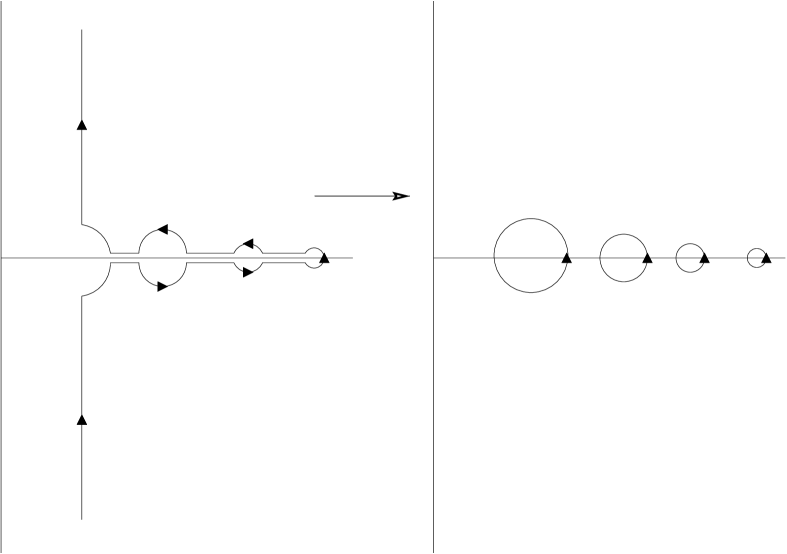
Figure 1: Contour deformation for isolated singularities.

with the contour $C_{\infty}$ encircling $\beta=\infty$ clockwise. Given the analytic structure of the canonical partition function as explained in the previous section, we can estimate $\Omega(E)$ in a high-energy expansion by contour deformation through the singularities of $Z(\beta)$. The original contour $C_{\infty}$ can be split into pieces running close to the singularities (encircling counter-clockwise the singularities if they are isolated, as in figure (1), or the cuts if they are branch-points), $C_{\infty}=\cup_{\alpha}C(\beta_{\alpha})$.

In the ideal-gas or one-loop approximation the total density of states factorizes in sectors:

$$\Omega=\Omega_{\rm closed}\cdot\prod_{(p,q)}\Omega_{{\rm D}p-{\rm D}q}+2\;{\rm loop}.$$ (66)

In a given sector, the density of states is then written as a sum $\Omega=\sum_{\alpha}\Omega_{\alpha}$, each term being dominated by the behaviour of $Z(\beta)$ near the singularity $\beta_{\alpha}$

$$\Omega_{\alpha}\approx e^{\beta_{\alpha}\,E+a_{\alpha}\,V_{\parallel}}\;\int_{C_{\alpha}}{\mbox{d}\beta\over 2\pi i}\;e^{(\beta-\beta_{\alpha})(E-\rho_{\alpha}\,V_{\parallel})}\;Z_{{\rm sing},\alpha}$$ (67)

where we have used the Taylor expansion (43) of the regular part of the free energy ${\rm log}\,Z_{{\rm reg},\alpha}$ to leading order

$${\rm log}\,Z_{{\rm reg},\alpha}\sim a_{\alpha}\,V_{\parallel}-\rho_{\alpha}\,V_{\parallel}\,(\beta-\beta_{\alpha})+{\cal O}\left(V_{\parallel}\,(\beta-\beta_{\alpha})^{2}\right).$$ (68)

The quantity $\rho_{\alpha}\sim{\cal O}(1)$ in string units, is a critical Hagedorn density on the relevant volume for each sector. The smallness of the neglected higher order terms in (68) must be checked in each situation.

The singular part for open-string systems takes the form

$${\rm log}\,Z_{{\rm sing},\alpha}\sim\frac{1}{2}\,C_{\gamma}\,g_{\alpha}\,f\,\left(\beta-\beta_{\alpha}\right)^{\gamma}\;\left[{\rm log}\,\left(\beta-\beta_{\alpha}\right)\right]^{\delta},$$ (69)

with $g_{\alpha}$ is the degeneracy of the critical eigenvalue $\lambda_{\alpha}$, $\delta=1$ if $\gamma$ is a positive (or zero) integer, and $\delta=0$ otherwise. The constant

$$C_{\gamma}\propto\left\{\begin{array}[]{ll}\Gamma(-\gamma)\;,&\gamma\notin{\bf Z}^{+}\cup\{0\}\\ \\ {(-1)^{\gamma+1}\over\Gamma(\gamma+1)}\;,&\gamma\in{\bf Z}^{+}\cup\{0\}.\end{array}\right.$$

The volume factor

$$f={V_{\parallel}\over V_{\perp}},$$ (70)

and the critical exponent $\gamma=-1$. Formula (69) may also be used for closed strings, where $\gamma=0,\delta=1$, and the absolute normalization is obtained setting $f=1$.

The Dominance Rule of the Hagedorn Singularity

The condition that the full density of states is dominated by the contribution from the Hagedorn singularity $\beta_{0}=\beta_{c}=2\pi\sqrt{2}$ is

$${\rm log}\,(\Omega_{c}/\Omega_{1})\gg 1,$$ (71)

with $\Omega_{1}$ the contribution to the density of states from the closest singularity to $\beta_{c}$, which we shall denote $\beta_{1}$. In all the situations considered in the present work, $\beta_{1}$ is real and $\beta_{1}<\beta_{c}$. A necessary condition is obtained from the leading exponential behaviour of (67)

$$\beta_{c}\,E+a_{c}\,V_{\parallel}\gg\beta_{1}\,E+{\rm Re}(a_{1})\,V_{\parallel}$$ (72)

or, estimating the coefficient ${\rm Re}(a_{1})\approx a_{0}+\rho_{c}^{\prime}\,(\beta_{c}-\beta_{1})$ in a Taylor expansion around $\beta_{c}$, with $\rho_{c}^{\prime}={\cal O}(1)$ in string units,

$$(\beta_{c}-\beta_{1})(E-\rho_{c}^{\prime}\,V_{\parallel})\gg 1.$$ (73)

This is a necessary condition, albeit not sufficient, as we will learn later on in this section. Again note that this is a condition involving the energy density on the brane (or intersection).

If the next-to-leading singularity $\beta_{1}$ is independent of the T-moduli, then $\beta_{c}-\beta_{1}\sim{\cal O}(1)$ and condition (73) reduces to the requirement of large energy densities in the relevant world-volume ($V_{D-1}$ for closed strings or $V_{\parallel}$ for open strings):

$$\rho\equiv{E\over V_{\parallel}}\gg{\cal O}(1)$$ (74)

in string units. We shall always work in this regime.

However, in many cases $\beta_{1}$ depends on the T-moduli. For example, if some $R_{\perp}\gg 1$ in open-string systems, we have $\beta_{c}-\beta_{1}\sim 1/R_{\perp}^{2}$ as in (39), and (73) depends non-trivially on the DD moduli. If $R_{\perp}$ is sufficiently large for a given total energy, the condition (73) is violated. In this case, it is a better approximation to evaluate the density of states in the non-compact limit $R_{\perp}\sim\infty$, which corresponds to the radius-dependent singularities coalescing with the Hagedorn singularity, changing the critical exponent according to

$$\gamma\rightarrow\gamma_{\infty}=\gamma+{d_{\infty}\over 2},$$ (75)

with $d_{\infty}$ the number of such ‘non-compact’ dimensions. The volume factor in (69) also changes by removing from $V_{\perp}$ the volume of the ‘non-compact’ dimensions. For example, if all $d_{\perp}$ large DD directions are to be approximated as non-compact, we have

$$f\rightarrow f_{\infty}\sim V_{\parallel}.$$ (76)

Thus, we handle the violation of (73) by a change in the critical exponent $\gamma$. After this, the remaining closest singularity is independent of the DD radius and is separated a distance of ${\cal O}(1)$ in string units.

In the context of these approximation techniques, we shall discuss the evaluation of the basic integral (67) for a general value of the critical exponent $\gamma$. A change of variables gives the following expression for the Hagedorn singularity contribution:

$$\Omega_{c}\approx e^{\beta_{c}\,E+a_{c}\,V_{\parallel}}\cdot\omega_{\gamma}\cdot\int_{C(\beta_{c})}{\mbox{d}z\over 2\pi i}\,{\rm exp}\left\{x_{\gamma}\,(z+C_{\gamma}\,z^{\gamma}\,[{\rm log}\,(z\,\omega_{\gamma})]^{\delta})\right\},$$ (77)

where

$$\omega_{\gamma}\equiv\left({x_{\gamma}\over f}\right)^{1/\gamma}\qquad z={\beta-\beta_{c}\over\omega_{\gamma}}$$ (78)

and the parameter $x_{\gamma}$ is defined by

$$x_{\gamma}\equiv f\,\left({E-\rho_{c}\,V_{\parallel}\over f}\right)^{\gamma\over\gamma-1}=f\,[V_{\perp}\,(\rho-\rho_{c})]^{\gamma\over\gamma-1}.$$ (79)

It is important to keep in mind that, while $\beta_{c}$ is a universal constant for all open and closed sectors, the ‘ground state degeneracy’ $a_{c}$, and the critical energy density $\rho_{c}$ are sector-dependent, both dimensionally and numerically.

The representation (77) of the Hagedorn singularity contribution is well-suited for the presentation of the two most useful approximation techniques in the evaluation of $\Omega(E)$, which we now discuss.

Saddle Point

Written in the form (77), we see that the saddle-point approximation is good if $x_{\gamma}\gg 1$, provided the neglected terms in the Taylor expansion of the regular free energy, of order

$$V_{\parallel}\,(\beta-\beta_{c})^{2+n}\sim V_{\parallel}\cdot{(x_{\gamma})^{2+n}\over(E-\rho_{c}\,V_{\parallel})^{2+n}}\,z^{2+n}$$ (80)

are small. These terms produce a negligible shift of the saddle point at $z=z_{s}\sim{\cal O}(1)$ if

$${V_{\parallel}\;(x_{\gamma})^{1+n}\over(E-\rho_{c}\,V_{\parallel})^{2+n}}\sim V_{\perp}\,[V_{\perp}\,(\rho-\rho_{c})]^{2+n-\gamma\over\gamma-1}\ll 1.$$ (81)

So, given that we are interested in Hagedorn densities in the world-volume $\rho>\rho_{c}$, and $V_{\perp}\geq 1$ by construction, we see that, as soon as $\gamma>1$, (81) is violated at sufficiently high order in the Taylor expansion. Thus, the saddle-point approximation is not applicable to the full integral for $\gamma>1$, even if $x_{\gamma}\gg 1$.

On the other hand, for $\gamma<1$ and $x_{\gamma}\gg 1$, the analytic corrections are under control and the saddle-point approximation is good, leading to a Hagedorn-dominated density of states of the form

$$\Omega(\gamma<1)_{\rm saddle}\approx{\omega_{\gamma}\;e^{\beta_{c}\,E+a_{c}\,V_{\parallel}+{\gamma-1\over\gamma}\,z_{s}\,x_{\gamma}+\Delta_{s}}\over\sqrt{x_{\gamma}}}\;\left[1+{\cal O}\left({\Delta_{s}\over x_{\gamma}}\right)+{\cal O}\left({1\over x_{\gamma}}\right)\right]$$ (82)

for $\gamma\neq 0$. The quantity $\Delta_{s}$ in the exponent is of order

$$\Delta_{s}\sim V_{\parallel}\,(\beta_{s}-\beta_{c})^{2}\sim{(x_{\gamma})^{2}\over V_{\parallel}(\rho-\rho_{c})^{2}}\sim{V_{\parallel}\over[V_{\perp}(\rho-\rho_{c})]^{2-\gamma\over 1-\gamma}},$$ (83)

and accounts for the small shift (81) of the saddle-point at $\beta_{s}$ by the neglected analytic corrections to the free energy. The first correction term in square brackets comes from the effect of these analytic terms in the evaluation of the saddle-point integral, while the second one is a ‘two-loop’ correction term, controlled by the small parameter $1/x_{\gamma}$.

The saddle-point approximation leads to the equivalence with the canonical ensemble, so that these results are compatible with the contents of table (1), where $\gamma=1$ is the maximum critical exponent admitting a canonical analysis.

By explicit inspection of the saddle-point equation, one can check that the dominant saddle point (the one with largest real part) for all values of $\gamma<1$ of the form (75) has $z_{s}$ real and positive, so that there are large exponential contributions to $\Omega_{c}$ for $\gamma<0$ in the saddle-point, $x_{\gamma}\gg 1$, limit. This implies a refinement of the condition (73). The contribution from the next-to-leading singularity $\beta=\beta_{1}$ to the entropy is also linear in $x_{\gamma}$ and it differs from the Hagedorn one by the replacement

$$x_{\gamma}\rightarrow(g_{1})^{1/1-\gamma}\,x_{\gamma},$$ (84)

with $g_{1}$ the multiplicity of the singularity at $\beta_{1}$. For the DD-moduli-dependent singularities (45) we have $g_{1}>1$ and the condition (73) must be refined to

$$(\beta_{c}-\beta_{1})(E-\rho_{c}^{\prime}\,V_{\parallel})\gg\left\{\begin{array}[]{ll}{\rm max}\,(1,x_{\gamma})&{\rm if}\;\;\;\;{\gamma<0}\\ 1&{\rm if}\;\;\;\;{\gamma\geq 0.}\end{array}\right.$$

We shall refer to this condition as the Hagedorn-dominance-rule (H.d.r.). Notice that it is equivalent to the requirement that the saddle-point (canonical) temperature be ‘close’ to the Hagedorn temperature: $|\beta_{c}-\beta_{s}|\ll|\beta_{c}-\beta_{1}|$. If condition (3.1) is violated, one has to change the critical exponent $\gamma$ according to (75) and the conditions for single-singularity dominance in the new regime must be considered.

If $\gamma=0$, the ‘loop-expansion parameter’ $x_{0}=x_{\gamma=0}=f$, independent of the energy, and we find

$$\Omega(\gamma=0)_{\rm saddle}\approx{e^{\beta_{c}\,E+a_{c}\,V_{\parallel}+f+\Delta_{s}}\over\sqrt{f}}\;\left({E-\rho_{c}\,V_{\parallel}\over f}\right)^{f-1}\;\left[1+{\cal O}\left({\Delta_{s}\over x_{0}}\right)+{\cal O}\left({1\over x_{0}}\right)\right],$$ (85)

with $\Delta_{s}$ as in (83) with $\gamma=0$.

All the systems with $\gamma<1$, whose behaviour is well approximated by a saddle point, $x_{\gamma}\gg 1$, show canonical thermodynamic behaviour, as in table (1). For these systems the internal energy diverges at the Hagedorn temperature, which can be considered as limiting. We shall denote these systems as ${\bf L}[\gamma]$.

No Saddle Point

If the conditions for the saddle-point approximation are not satisfied, that is, we have $\gamma>1$ or we have $x_{\gamma}\ll 1$ for $\gamma<1$, then we can try a complementary approximation to the integral, with effective expansion parameter $(x_{\gamma})^{1-\gamma}$. That is, we have an expansion which is good if $x_{\gamma}\ll 1$ for $\gamma<1$, and $x_{\gamma}\gg 1$ if $\gamma>1$. In all cases of interest except $\gamma=-1$, the partition function has a branch-point at the Hagedorn singularity. By evaluating the discontinuity of the integrand across the cut, we can transform the $z$-integral (77) into (for $\gamma$ not an integer)

$${1\over x_{\gamma}}\,\int_{0}^{u_{1}}{\mbox{d}u\over\pi}\,{\rm exp}\left\{-u+C_{\gamma}\,(x_{\gamma})^{1-\gamma}\,{\rm cos}\,(\pi\gamma)\,u^{\gamma}\right\}\;\;{\rm sin}\,\left\{C_{\gamma}\,{\rm sin}\,(-\pi\gamma)\,(x_{\gamma})^{1-\gamma}\,u^{\gamma}\,\right\},$$ (86)

with

$$u_{1}\equiv(\beta_{c}-\beta_{1})(E-\rho_{c}\,V_{\parallel})\gg 1,$$ (87)

within the Hagedorn-singularity-dominance regime. On approximating (77) by (86) we are neglecting the contribution of a small circle in the contour around $\beta=\beta_{c}$. This is justified for $\gamma>0$, where the partition function is bounded near the singularity. The cases $\gamma=-1,0$ will be dealt with exactly below, while $x_{-1/2}\gg 1$ in all practical cases treated below, so that $\gamma=-1/2$ is calculable in the saddle-point approximation.

The integral (86) admits a perturbative expansion in $(x_{\gamma})^{1-\gamma}$ with a leading term of order $1/(x_{\gamma})^{\gamma}$. The result is equivalent to the single-long-string picture in table (1), with a density of states:

$$\Omega_{\rm long}\approx f\cdot{e^{\beta_{c}\,E+a_{c}\,V_{\parallel}}\over(E-\rho_{c}\,V_{\parallel})^{1+\gamma}}\;\left[1+{\cal O}\left({1\over V_{\parallel}(\rho-\rho_{c})^{2}}\right)+{\cal O}\left({f\over(E-\rho_{c}\,V_{\parallel})^{\gamma}}\right)\right].$$ (88)

If the critical exponent is an integer, $\gamma=k\geq 2$, the integral (86) is replaced by

$${1\over x_{k}}\,\int_{0}^{u_{1}}{\mbox{d}u\over\pi}\,{\rm exp}\left\{-u+(x_{k})^{1-k}\,u^{k}\,{\rm log}\left({E-\rho_{c}\,V_{\parallel}\over u}\right)\right\}\;\;{\rm sin}\,\left\{\pi\,(x_{k})^{1-k}\,u^{k}\,\right\},$$ (89)

with the same leading behaviour as (88), but now with corrections of

$${\cal O}\left((x_{k})^{1-k}\,{\rm log}\,(E-\rho_{c}\,V_{\parallel})\right)\sim{\cal O}\left({f\over(E-\rho_{c}\,V_{\parallel})^{k}}\;{\rm log}\,(E-\rho_{c}\,V_{\parallel})\right).$$

This regime is equivalent to Eq. (62), or table (1) with $\gamma>1$. The formally defined temperature $\beta=\partial{\rm log}(\Omega)/\partial E$ is larger than the Hagedorn temperature. Although the thermodynamics of these systems is ill-defined, there is nothing wrong in principle with the density of states (88) at finite volume, and we will use the ‘thermodynamic’ language and denote these systems as ‘non-limiting’, or ${\bf NL}[\gamma]$.

As well as these approximations, there are a number of special cases which can be evaluated for all $x_{\gamma}$. The first and most interesting for our discussion is $\gamma=-1$. Since this case corresponds to open strings in a finite volume, which is naturally of central importance to our discussion, we shall evaluate this case separately in subsection 3.3. The two other interesting cases we shall consider now; they are $\gamma=0$ and $\gamma=1$.

Special Case $\gamma=0$

The special case $\gamma=0$ admits exact evaluation of the integral (77), resulting in

$$\Omega(\gamma=0)_{c}\sim{1\over\Gamma(f)}\,{e^{\beta_{c}\,E+a_{c}\,V_{\parallel}}\over(E-\rho_{c}\,V_{\parallel})^{1-f}}\,\left[1+{\cal O}\left({f\over V_{\perp}\,(\rho-\rho_{c})^{2}}\right)-{\cal O}\left(e^{-u_{1}}\right)\right],$$ (90)

the first correction factor coming from the analytic terms around the Hagedorn singularity, and the second one coming from the next-to-leading singularity $\beta_{1}$. This formula interpolates between the saddle-point result (85), ${\bf L}[0]$, valid at $x_{0}=f\gg 1$, and the form (88) of ${\bf NL}[0]$ type, for $f\ll 1$.

In the marginal case $f=1$, corresponding to closed strings, the limiting or non-limiting behaviour is controlled by the sign of the correction terms. In this case, the singularities are isolated poles of the partition function, and the sign of the next-to-leading singularity correction should be negative, leading to a weakly limiting behaviour that will be studied in more detail in the next subsection.

Special Case $\gamma=1$

Finally, we consider the special case $\gamma=1$, where the parametrization (77) fails. The singular part of the free energy takes the form

$${\rm log}\,Z_{\rm sing}\sim f\,(\beta-\beta_{c})\,{\rm log}\,(\beta-\beta_{c}).$$ (91)

In the saddle-point approximation, the critical point is located at

$${\rm log}\,(\beta_{s}-\beta_{c})=-{E-\rho_{c}\,V_{\parallel}\over f}-1,$$ (92)

and the resulting canonical determination of the density of states is:

$$\Omega(\gamma=1)_{\rm saddle}\approx{1\over\sqrt{f}}\;{\rm exp}\,\left\{\beta_{c}\,E+a_{c}\,V_{\parallel}-f\,e^{-{E-\rho_{c}\,V_{\parallel}\over f}-1}-\frac{1}{2}\left(1+{E-\rho_{c}\,V_{\parallel}\over f}\right)+\Delta_{s}\right\}.$$ (93)

On evaluating $\beta$, one finds the marginal case of logarithmically limiting behaviour seen in table (1). We shall refer to this type of density of states as ${\bf L}[1]$.

In fact, the saddle-point approximation has a limited range of applicability, since ‘higher-loop’ corrections are of ${\cal O}(1/f(\beta_{s}-\beta_{c}))$ and thus we may define the saddle-point control parameter $x_{1}\sim f(\beta_{s}-\beta_{c})$:

$$x_{1}\equiv f\;e^{-{E-\rho_{c}\,V_{\parallel}\over f}}=f\,e^{-V_{\perp}(\rho-\rho_{c})},$$ (94)

the saddle-point approximation being good for $x_{1}\gg 1$. The analytic corrections are of order

$${\Delta_{s}\over x_{1}}\sim{\cal O}\left(V_{\perp}\,e^{-V_{\perp}(\rho-\rho_{c})}\right).$$

In the opposite limit, $x_{1}\ll 1$, a similar treatment to the one in Eq. (89) gives

$$\Omega(\gamma=1)_{\rm long}\approx{f\over(E-\rho_{c}\,V_{\parallel}-f\,{\rm log}\,f\,)^{2}}\;{\rm exp}\left\{\beta_{c}\,E+a_{c}\,V_{\parallel}\right\},$$ (95)

which is of ‘non-limiting’ type: ${\bf NL}[1]$, with corrections of

$${\cal O}\left({1\over V_{\parallel}(\rho-\rho_{c}-V_{\perp}^{-1}\,{\rm log}\,(f))^{2}}\right)+{\cal O}\left[\left({f\over E-\rho_{c}V_{\parallel}-f{\rm log}(f)}\right){\rm log}\left({E-\rho_{c}V_{\parallel}-f{\rm log}(f)\over f}\right)\right].$$

3.2 Closed Strings in a Finite Box

Using these methods, we can now review the results of Ref. [8] for closed strings. Let us consider a box of radius $R\geq 1$, with volume $V_{D-1}\sim R^{D-1}$. The corresponding analytic structure is given in Eq. (58), and we can explicitly evaluate the integral (67) with the result

$$\Omega_{\rm closed}=\sum_{\alpha}(\beta_{\alpha})^{k_{\alpha}}\,{e^{\beta_{\alpha}\,E+a_{\alpha}\,V_{D-1}}\over(k_{\alpha}-1)!}\;(E-\rho_{\alpha}\,V_{D-1})^{k_{\alpha}-1}\;\left[1+{\cal O}\left({(k_{\alpha}-1)(k_{\alpha}-2)\over V_{D-1}(\rho-\rho_{\alpha})^{2}}\right)\right].$$ (96)

The corrections come from the analytic terms around each pole, and are absent for the leading Hagedorn singularity, since $k_{c}=1$. From the analysis of Ref. [8] we learn that the next-to-leading singularity of the partition function $\beta_{1}$ is a pole of order $k_{1}=2D-2$, located at

$$\beta_{c}-\beta_{1}=\eta/R^{2},$$ (97)

with $\eta\sim+{\cal O}(1)$ in string units. The Hagedorn-dominance-rule (H.d.r.) of Eq. (3.1) is given by

$$(\rho-\rho_{c}^{\prime})\,R^{D-3}\gg 1,$$ (98)

which is satisfied for moderately high energy density $\rho>\rho_{c}^{\prime}$ and large radius, provided $D>3$, or for small radius but very high energy density $\rho\gg 1$. In these conditions, the density of states is approximated by

$$\Omega_{\rm closed}\approx\beta_{c}\;e^{\beta_{c}\,E+a_{c}\,V_{D-1}}\left[1-\frac{(\beta_{c}\,V_{D-1})^{2D-3}}{(2D-3)!}\,\rho^{2D-3}\;{\rm exp}\left\{-\eta\,R^{D-3}\,(\rho-\rho^{\prime}_{c})\right\}\right],$$ (99)

Now, in accord with our heuristic argument, in the limit of large $R$ and provided that the energy density is larger than the Hagedorn density, the energy dependence of the microcanonical density of states always resembles that for a small compact system no matter how large the volume we consider. Eq. (98) is precisely the condition $E\gg\varepsilon_{0}$, and tells us the energy scale above which some of the strings are able to feel the compactness of the large dimensions by winding.

On using the microcanonical density of states to find the temperature (from $\beta=\partial\log\Omega/\partial E$) we find

$$E\approx\rho^{\prime}_{c}V_{D-1}-R^{2}\,\log\left((\beta_{c}E)^{3-2D}\,R^{2}(\beta-\beta_{c})\right).$$ (100)

In particular the specific heat,

$$C_{V}\approx{R^{2}\over\beta-\beta_{c}},$$ (101)

is always positive and the Hagedorn temperature is approached monotonically from below. Therefore, for closed strings in finite volume, the Hagedorn temperature is logarithmically limiting, even in the thermodynamic limit for $D>3$. Notice that this limiting behaviour is very weak, since we can rise the temperature arbitrarily close to the Hagedorn temperature, while maintaining a moderately low energy density, provided $R$ is large enough. For future reference, we shall denote this behaviour as ‘marginally limiting’: ${\bf ML}$.

When $D\leq 3$ the H.d.r. is violated at sufficiently large $R$. In this case we must use the approximation of non-compact $D_{\infty}-1\leq 2$ dimensions, the saddle-point approximation is good, and we get standard ${\bf L}[(D_{\infty}-1)/2]$ behaviour, in agreement with the canonical ensemble, and the results of table (1). For these lower-dimensional systems there is not enough energy available to excite winding modes.

3.3 Open Strings on D-branes in a Finite Box

Now we are ready to present new results for D-brane systems. Since the critical exponent $\gamma=-1$ and the volume factors are independent of the ND$+$DN moduli, the discussion can be done in general for all values of $\nu$, as a function of the number of large DD directions, $d_{\perp}$, and the volumes $V_{\perp},V_{\parallel}$.

The control parameter for the saddle-point approximation is

$$x_{-1}\equiv x=V_{\parallel}\sqrt{\rho-\rho_{c}\over V_{\perp}}$$ (102)

and the H.d.r. (3.1) for $x\gg 1$ is

$$1\ll{u_{1}\over x}\sim\sqrt{\rho-\rho_{c}}\;\left(R_{\perp}\right)^{-2+d_{\perp}/2}.$$ (103)

So, for the very high-energy regime

$${\rm max}\,\left(\rho_{c}\,,{V_{\perp}\over V_{\parallel}^{2}}\,,R_{\perp}^{4-d_{\perp}}\right)\ll\rho$$ (104)

we find ${\bf L}[-1]$ behaviour. In particular, this includes all systems with $d_{\perp}=0$.

On the other hand, for $x\ll 1$, the $\gamma=-1$ H.d.r. condition reads

$$1\ll u_{1}\sim{(\rho-\rho_{c})\,V_{\parallel}\over R_{\perp}^{2}},$$ (105)

so that the intermediate range

$${\rm max}\,\left(\rho_{c}\,,{R_{\perp}^{2}\over V_{\parallel}}\right)\ll\rho\ll{V_{\perp}\over V_{\parallel}^{2}}$$ (106)

shows a new behaviour characterized by $\gamma=-1$ but $x\ll 1$. In fact, we can study the density of states at all values of $x$, since the integral (77) can be evaluated in closed form by deforming the contour to the steepest descent contour as shown in figure 1:

$$\Omega(\gamma=-1)_{c}=\beta_{c}\,f\;x^{-1}\;I_{1}(2x)\;e^{\beta_{c}\,E+a_{c}\,V_{\parallel}}\,\left[1+{\cal O}\left({x^{2}\over V_{\parallel}(\rho-\rho_{c})^{2}}\right)+{\cal O}\left(e^{-u_{1}}\right)\right],$$ (107)

where $I_{1}$ is the modified Bessel function of the first kind. The saddle-point regime $x\gg 1$ is equivalent to (82), and is therefore of ${\bf L}[-1]$ type, whereas the $x\ll 1$ region is marginal from the point of view of the long string picture (88). In fact, the exact expression (107) leads to rather standard thermodynamics in both extreme regimes in terms of the parameter $x$, with $x\sim 1$ marking a cross-over from long-string dominance on the brane to many windings in the transverse directions.

We can see this when we calculate the temperature. Defining

$$y=\frac{\beta-\beta_{c}}{f\beta_{c}},$$ (108)

we find

$$y=\frac{1}{2x}\left(\frac{I_{0}(2x)+I_{2}(2x)}{I_{1}(2x)}-\frac{1}{x}\right).$$ (109)

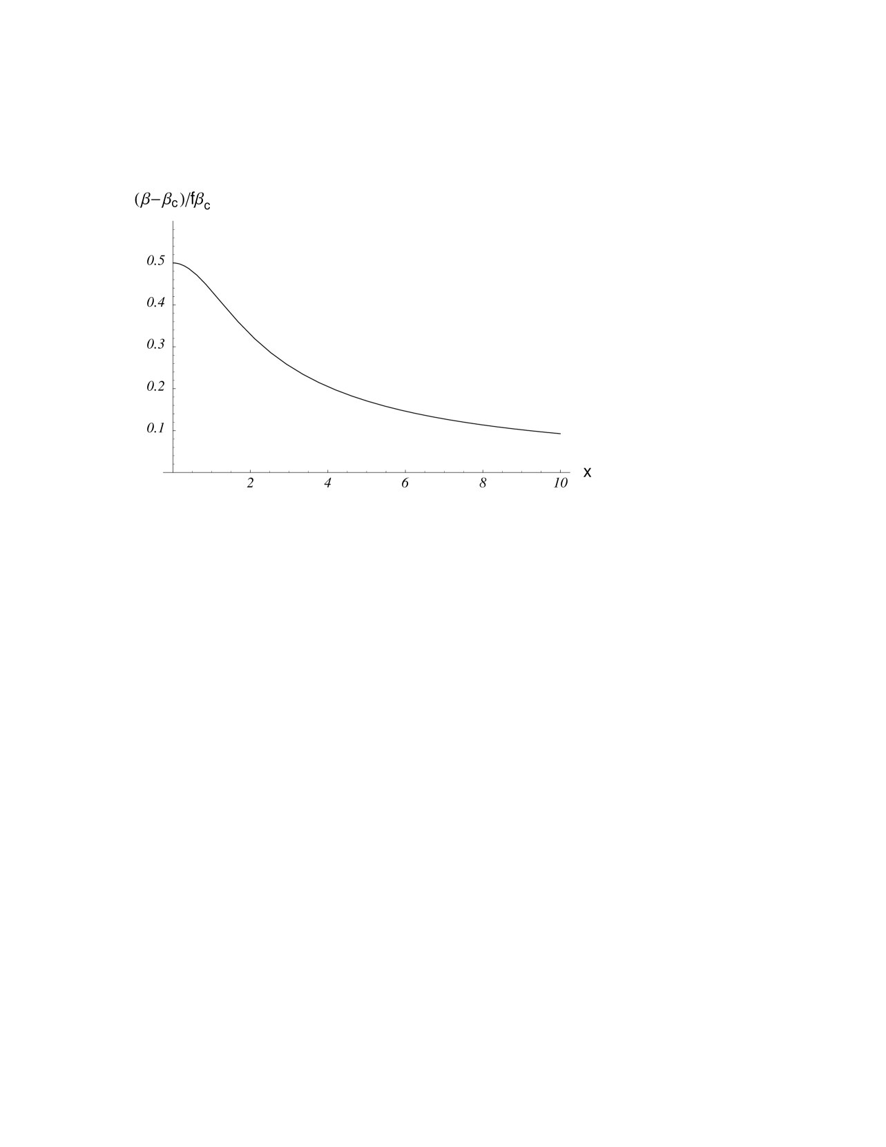
Figure 2: Variation of $\beta-\beta_{c}$ with $x=\sqrt{f\,(E-\rho_{c}\,V_{\parallel})}$ for open strings.

This function, shown in figure (2), has a tail towards large $x$ giving

$$\beta_{c}\,E\approx{f\beta_{c}^{2}\over(\beta-\beta_{c})^{2}}.$$ (110)

In the notation of table (1), this is equivalent to $\gamma=-1$ or $D_{o}=d_{NN}$. It is the behaviour of an open-string system which has all DD directions small and compact $(d_{\perp}=0)$, with both the energy and specific heat diverging as we approach the Hagedorn temperature. This was to be expected from the closed-string case, however small $x$ gives us a region of different behaviour.

When $x\,\raisebox{-2.58334pt}{$\buildrel<\over{\sim}$}\,1$, we find

$$E\approx\rho_{c}\,V_{\parallel}+\frac{6}{f\beta_{c}}-12\frac{(\beta-\beta_{c})}{f^{2}\beta_{c}^{2}}.$$ (111)

This has a small specific heat as we approach the Hagedorn temperature provided we can maintain small $x$. This new type of behaviour is equivalent to keeping the ${\cal O}(x^{2})+{\cal O}(x^{4})$ corrections in (88), and can be described as ‘weakly limiting’, due to its small specific heat at Hagedorn temperatures. We shall denote it by ${\bf WL}[-1]$.

We can obtain a microscopic understanding of this behaviour by examining the fraction of strings which have energy greater than the single-string threshold energy $\varepsilon_{0}$, and hence are able to wind. The energy distribution (i.e. the average number of strings in the gas with an energy in the interval $\varepsilon\rightarrow\varepsilon+\mbox{d}\varepsilon$ when the total energy of the system is $E$) is given by [8]

$${\cal D}(\varepsilon;E)\;\mbox{d}\varepsilon=\frac{\omega(\varepsilon)\Omega(E-\varepsilon)}{\Omega(E)}\mbox{d}\varepsilon.$$ (112)

The exponent appearing in $\omega$ depends on the effective dimension and hence on whether $\varepsilon$ is greater than or less than $\varepsilon_{0}$. Below $\varepsilon_{0}$, the distribution is peaked with a power law decay that is familiar from the closed-string case. Above $\varepsilon_{0}$ and for $x\gg 1$ we can approximate

$${\cal D}(\varepsilon;E)=f\;\beta_{c}\;e^{-\varepsilon\;x/E}.$$ (113)

Integrating this expression from $\varepsilon_{0}$ to $E$ gives the total number of energetic strings;

$$x\;e^{-\varepsilon_{0}\;x/E}.$$ (114)

Eq. (3.1) is equivalent to $E\gg\varepsilon_{0}$ and $x\ll E/\varepsilon$. Thus the total energy must always be larger than the nominal threshold energy required to excite winding modes. However the number of energetic strings is roughly proportional to $x$ and for $x\ll 1$ there are no winding modes, with all the energy being concentrated in short string excitations close to the D-brane. As we increase the value of $x$, by raising the energy for example, we find that a few of the open strings on the brane accumulate most of the energy in a manner which is similar to closed-string behaviour. As we increase $x$ still further, these strings are able to wind, and the spectrum becomes increasingly resolved into a low-energy peak and highly energetic winding modes. The average energy carried by strings in the low-energy peak becomes saturated as $x$ becomes large and $x\approx 1$ marks a cross-over in behaviour.

It is interesting to see what happens if we increase the volume of the brane. Since $\Omega$ is a monotonically increasing function of $V_{\parallel}$, there is always an entropic advantage in maximizing it. Hence the string gas is expected to spread itself over the whole available D-brane volume and the volume is expected to increase. As one might have expected (since there are no winding modes in the NN directions), for 9-branes the result is in accord with Ref. [12] (based on minimizing the free energy for 9-branes). However the windings in the DD-directions play an interesting role as can be seen by the fact that there is an entropic disadvantage in increasing $V_{\perp}$. Winding modes (and more generally finite size effects) are seen to prevent DD-directions expanding. A natural proposal is then that an interplay of these effects can stabilize some directions whilst allowing others to expand without limit. This is a topic we shall leave for future study.

If the H.d.r. with $\gamma=-1$ is not satisfied, i.e. if the inequalities (103) and (105) are violated, then we must approximate the density of states by that of a $\gamma_{\infty}=-1+d_{\infty}/2$ system. In this case, the control parameter for ${\bf L}/{\bf NL}$ behaviour is

$$x_{\infty}\sim\left\{\begin{array}[]{ll}V_{\parallel}\,(\rho-\rho_{c})^{\gamma_{\infty}/\gamma_{\infty}-1}&\gamma_{\infty}\neq 1\\ \\ V_{\parallel}\,e^{-(\rho-\rho_{c})}&\gamma_{\infty}=1.\end{array}\right.$$

One has ${\bf NL}[\gamma_{\infty}\leq 1]$ if $x_{\infty}\ll 1$, and ${\bf L}[\gamma_{\infty}\leq 1]$ if $x_{\infty}\gg 1$. On the other hand, for $\gamma_{\infty}>1$, one always has $x_{\infty}\gg 1$ and ${\bf NL}[\gamma_{\infty}>1]$.

There are two main regimes of this kind. The range

$${\rm max}\,\left(\rho_{c}\,,{V_{\perp}\over V_{\parallel}^{2}}\right)\ll\rho\ll R_{\perp}^{4-d_{\perp}},$$ (115)

which is only possible for $0<d_{\perp}<4$, leads to ${\bf L}[-1+d_{\perp}/2]$ with the exception of the regime $\rho\gg V_{\parallel}$ in $d_{\perp}=3$, which is ${\bf NL}[1/2]$ instead. Finally, for ‘low’ densities

$$\rho_{c}\ll\rho\ll{\rm min}\,\left({V_{\perp}\over V_{\parallel}^{2}}\,,{R_{\perp}^{2}\over V_{\parallel}}\right)$$ (116)

one gets ${\bf NL}[-1+d_{\perp}/2]$ for $d_{\perp}>4$ and ${\bf L}[-1+d_{\perp}/2]$ for $0<d_{\perp}\leq 4$, with two exceptions: the regimes $\rho\gg V_{\parallel}$ in $d_{\perp}=3$ and $\rho\gg{\rm log}\,(V_{\parallel})$ in $d_{\perp}=4$, where one finds also ${\bf NL}[-1+d_{\perp}/2]$ behaviour.

3.4 Summary

We may summarize the broad lines of our analysis by distinguishing the two main high-energy limits of interest.

Extreme High-Energy Limit

The extreme high-energy regime can be analyzed in simple terms for all systems. Physically, we expect that at energies much larger than any scale formed from the T-moduli parameters, the physics should be similar to the one of a nine-torus of string-scale size and $\beta_{c}\,E\gg 1$. Then, the H.d.r. condition (3.1) is trivially satisfied, since $\beta_{1}-\beta_{c}\sim{\cal O}(1)$. In such a situation, there is no clear distinction between NN and DD directions, as both are of the order of the string scale and are exchanged by T-duality. We have $\gamma=-1$ for the three basic systems of supersymmetric intersections: $\nu=0,4,8$. Thus, the high-energy regime $\beta_{c}\,E\gg 1$ corresponds universally to the ${\bf L}[-1]$ behaviour. Closed strings are described by the ${\bf ML}$ form (99). Therefore the entropies $S={\rm log}(\Omega_{c})$ read

$$S_{\rm open} \approx \beta_{c}\,E+2\sqrt{f\,E}+{\rm const.}-{\cal O}({\rm log}\,E)$$

$$S_{\rm closed} \approx \beta_{c}\,E+{\rm const.}-E^{16}\,e^{-\eta E}+{\cal O}(E^{15}\,e^{-\eta E}),$$ (117)

with $f,\eta\sim+{\cal O}(1)$. So, the open-string systems clearly dominate the finite-volume asymptotic entropy:

$$S_{\rm open}\gg S_{\rm closed}.$$ (118)

Thermodynamic Limit

In the thermodynamic limit, we scale $V_{\parallel}\rightarrow\infty$ with $\rho\equiv E/V_{\parallel}$ fixed and large in string units. Although this limit does not exist in a strict sense, we shall see in section 5 that very stringent conditions can be imposed on the string coupling constant such that regimes of approximate thermodynamic behaviour can be defined. So we proceed with the analysis and find a large variety of behaviours, depending on the role played by the winding modes. Roughly speaking, if the winding modes are sufficiently quenched, one gets agreement with the results presented in table (1). On the other hand, if the scaling of the DD directions is such that winding modes store a sizeable portion of the energy, the behaviour differs from table (1) and one finds a general tendency towards restoration of limiting behaviour.

The two main types of behaviour are the single-long-string or ${\bf NL}$ behaviour, with entropy density $\sigma\equiv S/V_{\parallel}$ of the form (we keep only the leading terms in the thermodynamic limit)

$$\sigma_{{\bf NL}[\gamma]}\approx\beta_{c}\,\rho-{1+\gamma\over V_{\parallel}}\,{\rm log}\,(\rho),$$ (119)

and the various types of ‘limiting’ behaviour ${\bf L}[\gamma]$ (dominated by a saddle point)

$$\sigma_{{\bf L}[\gamma]}\approx\left\{\begin{array}[]{ll}\beta_{c}\,\rho+2\sqrt{\rho/V_{\perp}}&{\rm if}\;\;\;\;{\gamma=-1}\\ \\ \beta_{c}\,\rho\,+\,{\gamma-1\over\gamma}\,\rho^{\gamma\over\gamma-1}&{\rm if}\;\;\;\;{\gamma=-\frac{1}{2},\frac{1}{2}}\\ \\ \beta_{c}\,\rho+{\rm log}\,(\rho)&{\rm if}\;\;\;\;{\gamma=0}\\ \\ \beta_{c}\,\rho-e^{-\rho}&{\rm if}\;\;\;\;{\gamma=1,}\end{array}\right.$$

up to positive constants of ${\cal O}(1)$ in string units.

The case $d_{\perp}=0$ is always ${\bf L}[-1]$. There is universal agreement with the canonical ensemble results of table (1) for $0<d_{\perp}<4$, (for example, a D$p$-brane in ten dimensions with $p\geq 6$, or a D0–D8 intersection in ten non-compact dimensions). For $d_{\perp}>4$ however (D$p$-branes in ten dimensions with $p<5$), it matters whether the winding modes are quenched, $V_{\parallel}\ll R_{\perp}^{2}$, giving ${\bf NL}$ behaviour, or activated into a ${\bf L}[-1]$ system for $V_{\parallel}\,\raisebox{-2.58334pt}{$\buildrel>\over{\sim}$}\,\sqrt{V_{\perp}}$. There is an interesting intermediate window, $R_{\perp}^{2}\,\raisebox{-2.58334pt}{$\buildrel<\over{\sim}$}\,V_{\parallel}\ll\sqrt{V_{\perp}}$, of ${\bf WL}[-1]$ behaviour (106), with entropy density

$$\sigma_{{\bf WL}[-1]}\approx\beta_{c}\,\rho+{\beta_{c}\,f\over 2}\,\rho-{\beta_{c}^{2}\,V_{\parallel}\,f^{2}\over 24}\,\rho^{2}.$$ (120)

The critical case $d_{\perp}=4$ (a D5-brane in ten dimensions), is ${\bf L}[1]$, as in table (1) for sufficiently large transverse volume, namely $V_{\parallel}\ll\sqrt{V_{\perp}}$, and is ${\bf L}[-1]$ in the opposite regime $\sqrt{V_{\perp}}\,\raisebox{-2.58334pt}{$\buildrel<\over{\sim}$}\,V_{\parallel}$.

Finally, closed strings in the thermodynamic limit have a critical dimension $D=3$. For $D\leq 3$, we get standard canonical behaviour as in the table (1), ${\bf L}[(D-1)/2]$. On the other hand, for $D>3$ winding modes are important enough to turn the naive ${\bf NL}$ behaviour announced in table (1) into the ‘marginally limiting’ behaviour ${\bf ML}$ with entropy density

$$\sigma_{\bf ML}\approx\beta_{c}\,\rho-\rho^{2D-3}\,(V_{D-1})^{2D-4}\,e^{-\rho\,R^{D-3}}.$$ (121)

We see a tendency of the microcanonical, finite-volume analysis to restore limiting behaviour in the thermodynamic limit, even if the naive canonical ensemble determination predicted non-limiting features. There are a number of exceptions though, in which ${\bf NL}$ behaviour survives. Because negative specific heat systems are often signals of the breakdown of a given microscopic picture, it is worth collecting here all instances in which they appear. At finite ten-dimensional volume, ${\bf NL}$ behaviour only shows up for moderately ‘low’ energies, such that winding modes are quenched, i.e. the situation is analogous to that of closed strings. Examples are transient regimes with $d_{\perp}\geq 3$ (which restricts to $\nu=0,4$):

$${\rm max}\,\left(\rho_{c}\,,\,V_{\parallel}\,,{V_{\perp}\over V_{\parallel}^{2}}\right)\ll\rho\ll R_{\perp}$$ (122)

in a $d_{\perp}=3$ system (a D6-brane). It disappears if the transverse space is non-compact from the outset. The generic ${\bf NL}$ behaviour appears in the regime

$$\rho_{c}\ll\rho\ll{\rm min}\,\left({V_{\perp}\over V_{\parallel}^{2}}\,,{R_{\perp}^{2}\over V_{\parallel}}\right)$$ (123)

with $d_{\perp}>4$. The prototype system is a finite D$p$-brane in non-compact transverse space with $p<5$ (as in [19]). The very high energy-density regime of D6-branes $(\rho\gg V_{\parallel})$, and D7-branes $(\rho\gg{\rm log}\,(V_{\parallel}))$ in non-compact transverse space is also ${\bf NL}$. It is important to notice that all the ${\bf NL}$ regimes described here are transients for finite ten-dimensional volume. They become truly asymptotic regimes only in the case that DD directions are strictly non-compact (which is unphysical unless we manage to decouple closed strings).

We would like to note that the ${\bf L}$ behaviour, in which many long strings form, could indicate that, in an effective manner, the string tension vanishes.

4 Thermodynamic Balance

In this section we consider the behaviour of these systems when two or more of them are in thermal contact. For a given total energy $E_{\rm tot}$, we would like to find the most probable partition into components $E_{i}$, with

$$\sum_{i}E_{i}=E_{\rm tot}.$$ (124)

In the free approximation, we must maximize the total entropy

$$S(E_{\rm tot})=\sum_{i}S_{i}(E_{i})$$ (125)

under the constraint (124).

We have presented in the previous sections approximations for the functions $S_{i}(E_{i})$, valid in a given range of energies, so that the maximization problem is further restricted by the constraints:

$$E_{{\rm min},i}\ll E_{i}\ll E_{{\rm max},i}.$$ (126)

Conditions (124) and (126) determine the set ${\cal D}$ where a given form of the entropy functions is valid, and the maximization problem is defined. For example, we always restrict our treatment at least to the Hagedorn regime, $\rho_{i}>\rho_{c}$ for all components.

If a local maximum exists in the interior of ${\cal D}$, we have $\nabla S=0$ and the standard equilibrium condition of equality of temperatures,

$$T_{i}=T_{j},$$ (127)

with $T^{-1}_{i}=\beta_{i}=\partial S_{i}/\partial E_{i}$. In addition $\nabla^{2}S<0$, i.e. the specific heats are positive. If no local maximum is found in the interior of ${\cal D}$, the total entropy is maximized then on the boundary $\partial{\cal D}$. In this case, one or several components are pushed to extreme values of the energy, and the maximization process must be continued with the extension of the entropy functions to a different patch.

In principle, thermodynamic equilibrium of a single component with negative specific heat is possible when it is sufficiently large in magnitude, $|C^{-}_{V}|>C^{+}_{V}$, compared with that of normal systems [33]. Examples of this situation are familiar: large stars and black holes in equilibrium with radiation in a finite volume.

Therefore, it is tempting to suppose that our ${\bf NL}$ systems, with negative specific heats, can be in equilibrium with the normal systems under some conditions. However, the formally computed temperatures satisfy

$$T_{{\bf L}}<T_{c}<T_{\bf NL}.$$ (128)

Thus, they cannot be in equilibrium and the maximum entropy must occur on the boundary of ${\cal D}$. In particular, for the combined system with $S_{\rm tot}=S_{\bf L}+S_{\bf NL}$:

$${\partial S_{\rm tot}\over\partial E_{\bf NL}}=\beta_{\bf NL}-\beta_{\bf L}<0,$$ (129)

and $S_{\rm tot}$ is a monotonically decreasing function of $E_{\bf NL}$ throughout the entire Hagedorn regime. Therefore, the entropy is maximized by depleting ${\bf NL}$ energy in favor of the L system. Since we have at least one universal limiting system in any background: the closed strings, we can say that ${\bf NL}$ systems will have energy densities of the order of the string scale, which is the minimum energy density for which formula (119) holds. At this point the system of ${\bf NL}$ strings matches to the gas of massless states at Hagedorn densities.

Given that ${\bf NL}$ systems will be suppressed, we now turn to discuss the equilibrium conditions for the various ${\bf L}$ systems. From (3.4) we find the energy densities, as a function of the temperature

$$\rho_{{\bf L}[\gamma]}\approx\left\{\begin{array}[]{ll}V_{\perp}^{-1}\;(\beta-\beta_{c})^{-2}&{\rm if}\;\;\;\;{\gamma=-1}\\ \\ (\beta-\beta_{c})^{\gamma-1}&{\rm if}\;\;\;\;{-1<\gamma<1}\\ \\ -{\rm log}\,(\beta-\beta_{c})&{\rm if}\;\;\;\;{\gamma=1.}\end{array}\right.$$

So, close to the Hagedorn temperature, the ${\bf L}[\gamma]$ systems with smaller $\gamma$ have hierarchically larger energy densities.

The energy density of the ${\bf WL}[-1]$ system

$$\rho_{{\bf WL}}\approx{V_{\perp}\over V_{\parallel}^{2}}-2{V_{\perp}^{2}\over V_{\parallel}^{3}}\,(\beta-\beta_{c})$$ (130)

has a maximum of order $V_{\perp}/V_{\parallel}^{2}\gg 1$, according to (106). If this limit is exceeded, the density of states of such systems takes the ${\bf L}[-1]$ form. So, ultimately, very close to the Hagedorn temperature, the energy density in the form of ${\bf WL}$ systems is negligible compared to that in ${\bf L}$ systems.

The remaining system with a weak limiting behaviour is the closed-string sector with $D>3$, whose energy density satisfies

$$\rho_{{\bf ML}}\approx(2D-3)R^{3-D}\,{\rm log}\,\left(V_{D-1}\,\rho_{\bf ML}\right)-R^{3-D}\,{\rm log}\,\left(R^{2}(\beta-\beta_{c})\right).$$ (131)

This system is by far the weaker limiting system if $R$ is large enough, since Hagedorn temperatures can be achieved with $\rho\,\raisebox{-2.58334pt}{$\buildrel>\over{\sim}$}\,\rho_{c}\sim{\cal O}(1)$. The same condition for all the other systems requires $\rho_{\bf L}\rightarrow\infty$ or $\rho_{\bf WL}\sim V_{\perp}/V_{\parallel}^{2}\gg 1$. Therefore, we find the following hierarchy of energy densities in the thermodynamic limit:

$${\cal O}(1)\sim\rho_{\bf NL}\ll\rho_{\bf ML}\ll\rho_{\bf WL}\ll\rho_{\bf L}.$$ (132)

Within ${\bf L}$ systems, the one with smaller $\gamma$ wins. Similarly, within ${\bf NL}$ systems, the one with larger $\gamma$ is expected to lose energy faster when put in thermal contact with a ${\bf L}$ system.

In the extremely high-energy regime, both open and closed sectors are limiting. Using the forms in (3.4), we have again a clear dominance of the open-string sector. The energies in equilibrium satisfy

$$E_{\rm open}\approx{e^{2\,\eta\,E_{\rm cl}}\over(E_{\rm cl})^{34}},$$ (133)

so that we get the hierarchy

$${\cal O}(1)\ll E_{\rm closed}\ll E_{\rm open},$$ (134)

for $E>{\cal O}(10^{2})$. In the conclusions we shall discuss the possible implication for models of early cosmology.

There is another situation not covered by the previous discussion with some theoretical interest. Suppose we can completely decouple the closed-string and D-brane sectors at all energy scales (in particular at Hagedorn energy densities). This can be achieved by taking $N$ D$p$-branes in the large $N$ limit, with $g_{s}\,N<1$ and fixed. The effective open-string coupling remains finite while the open-closed and closed-closed coupling vanishes. In this case all extensive quantities in the open-string sector scale to leading order as ${\cal O}(N^{2})$ in the large $N$ limit. Then, if the transverse space is effectively non-compact and $\gamma_{\infty}>1$ we have a truly dominating ${\bf NL}$ system, because now it makes sense to concentrate only on the open-string sector, as totally decoupled from closed strings. In this situation we can consider the balance between two such ${\bf NL}$ systems. For example, in D0–D4 intersections with infinite DD directions, there is a balance between $\nu=0$ strings and $\nu=4$ strings, all of them ${\bf NL}$ in infinite transverse volume.

The maximization of the entropy of such a pair

$$S(E)\approx\beta_{c}\,E-(1+\gamma_{1})\,{\rm log}\,E_{1}-(1+\gamma_{2})\,{\rm log}\,E_{2},$$ (135)

under the condition $E_{1}\,,\,E_{2}>{\cal O}(1)$, at fixed $E=E_{1}+E_{2}$, is achieved with almost all the energy in the component with smallest $\gamma$. So, in the previous examples, $\nu=0$ systems with the largest possible world-volume dimensionality still store almost all the energy even if they are ${\bf NL}$.

5 Beyond the Ideal Gas Regime

In the previous sections we have studied aspects of Hagedorn regimes in various string systems, always in the ideal-gas approximation, given by the one-loop string diagrams. The question of the effect of interactions in the string thermodynamic ensemble is a notorious one. From a fundamental point of view, it is important to know what lies ‘beyond’ Hagedorn, under the assumption that there is some analogy with the QCD deconfining transition. Namely, is there a phase transition to a regime where ‘string constituents’ are liberated?

In the context of fundamental string theories this question is particularly elusive. For example, the presence of gravity automatically invalidates any naive discussion based on the canonical ensemble, or even the microcanonical ensemble in the thermodynamic (infinite volume) limit. Gravitational forces have long range and cannot be screened, so that extensivity cannot be taken for granted. Also, a finite energy density causes a back-reaction of the geometry. For a given total energy $E$, the largest volume that can be considered approximately static is the Jeans volume:

$$V_{\rm Jeans}\sim(G_{D}\,E)^{D-1\over D-3}$$ (136)

in $D-1$ spatial dimensions, with effective Newton constant $G_{D}$. The associated length scale $(V_{\rm Jeans})^{1/D-1}$ is the equivalent Schwarzschild radius for this energy. So, the idea that a black-hole phase lies ‘beyond’ Hagedorn (in the sense of large coupling or large energy) is rather natural. We shall pursue here this line of thought, without a precise specification of what the implications would be for a ‘constituent picture’ of the string.

A step in this direction is the correspondence principle of Ref. [24]. A wide variety of black holes in string theory can be adiabatically matched to various perturbative string states by appropriately choosing the string coupling constant. The matching point can be locally defined by the condition that the supergravity description of the black-hole horizon breaks down due to large $\alpha^{\prime}$-corrections. Then, both the mass and the entropy of the black hole can be matched at this point within ${\cal O}(1)$ accuracy of the coefficients. Under this correspondence, Schwarzschild black holes match onto highly excited (long) fundamental strings, whereas D-branes match onto qualitatively different kinds of black holes depending on the amount of energy on the D-brane world-volume. For a system of $N$ D$p$-branes at the same point in transverse space, the classical black-brane solution is characterized by two radii: a charge radius

$$(r_{Q})^{7-p}=g_{s}\,N$$ (137)

in string units, and the standard horizon radius $r_{0}$. In the near-extremal regime, $r_{0}\ll r_{Q}$, the black-brane state matches onto a thermal state of open-string massless excitations, i.e. the Yang–Mills gas on the D-brane world-volume. On the other hand, in the opposite Schwarzschild limit $r_{0}\gg r_{Q}$, the black brane matches onto a long-open-string state on the D-brane world-volume. The correspondence principle works in a variety of cases, and agrees with exact microscopic determinations of the black-hole entropy in those cases protected by supersymmetry.

These arguments are intended to apply to finite-energy states of the string theory defined by an asymptotic Minkowski vacuum. In particular, the perturbative long-string states are assumed to be mostly single-string states. On the other hand, the single-string-dominance picture of a stringy thermal ensemble suggests that perhaps the correspondence principle could be applied to the full thermal ensemble. Strictly speaking, such a statement cannot be literally true because of the ill-defined nature of the thermal ensemble in the presence of gravity. However, the microcanonical density of states calculated for all Hagedorn ensembles studied in this paper shows a leading linear behaviour for the entropy:

$$S(E)_{\rm Hag}=\beta_{c}\,E+{\rm subleading,}$$ (138)

just as in the single-string picture. Based on this, we shall propose that the correspondence principle applies provided the typical thermal state in the Hagedorn regime can be defined as an approximately stable state. The minimal requirement for this is to work at finite volume, well within the Jeans bound, and to use the microcanonical description. One then finds that at sufficiently high energy, for a given fixed value of the string coupling, the most likely state of the system is a black-brane or black-hole state. The condition that the energy does not exceed the Jeans bound is then equivalent to the requirement that a black hole of that mass fits inside the given volume. Thus, the Jeans bound, when applied to a finite-volume system, becomes roughly equivalent to the holographic bound (a black hole fills all the available volume, and the corresponding entropy gives the maximal information capacity of this background):

$$E<E_{\rm Hol}\sim{V^{D-3\over D-1}\over G_{D}}.$$ (139)

The interesting aspect of this mild extension of the correspondence principle is that the matching point (the transition from the perturbative string states to the black-states) is different from the Jeans bound. The correspondence point is defined by the matching of the entropies:

$$S(E)_{\rm Hag}\sim S(E)_{\rm black}.$$ (140)

This condition defines a critical energy as a function of the string coupling, different from the Jeans curve. Naively, this curve is just the transition line between a single long string and a single black hole. In the thermal gas however, we have seen many instances in which the thermal ensemble is not dominated by a single long string but the energy is distributed in a gas of long strings. In these cases, it may be reasonable to apply the correspondence principle to each individual string in the thermal gas. However, these subtleties are irrelevant to the level of accuracy we can achieve, because the correspondence matching itself is only known up to ${\cal O}(1)$ factors in the entropy and the energy. The distinctions between single-long-strings and multi-long-strings (${\bf NL}$ versus ${\bf L}$), or single- versus multi-black-holes, only show up in the subleading terms in the entropy, and are thus beyond our matching accuracy.

For a system of $N$ D$p$-branes with longitudinal volume $V_{\parallel}$ in a torus of nine-volume $V=V_{\parallel}V_{\perp}$, there are a number of ‘phases’ that can be identified on the basis of the correspondence principle, applied to the typical states both in the bulk and in the world-volume. That is, we label a ‘phase’ by those degrees of freedom with highest entropy, among those that coexist in the thermal ensemble for a given value of the moduli and the total energy.

5.1 Bulk Phase Diagram

A supergravity gas in ten dimensions has entropy

$$S(E)_{\rm sgr}\sim V^{1/10}\,E^{9/10}$$ (141)

and can be matched to a bulk black hole with entropy

$$S(E)_{\rm bh}\sim E\,(g_{s}^{2}\,E)^{1/7}.$$ (142)

The coexistence line $S_{\rm sgr}\sim S_{\rm bh}$ gives a black hole in equilibrium with radiation in a finite volume, with energy of order

$$E({\rm sgr}\leftrightarrow{\rm bh})\sim{1\over g_{s}^{2}}\,(g_{s}^{2}\,V)^{7/17},$$ (143)

and microcanonical temperature

$$T({\rm sgr}\leftrightarrow{\rm bh})\sim\left({1\over g_{s}^{2}\,V}\right)^{1/17}.$$ (144)

Since the black-hole-dominated region has negative specific heat, this temperature is maximal in the vicinity of the transition. This configuration is microcanonically stable in finite volume, in a range of energies between the matching point and the Jeans bound [34].

The graviton gas can also be matched to a gas of long closed strings. The coexistence curve $S_{\rm sgr}\sim S_{\rm Hag}$ at temperatures $T\sim{\cal O}(1)$ in string units, is independent of the string coupling and is given by the Hagedorn energy density:

$$E({\rm sgr}\leftrightarrow{\rm Hag})\sim V.$$ (145)

This Hagedorn phase can be exited at high energy or large coupling through the correspondence curve $S_{\rm Hag}\sim S_{\rm bh}$ (140):

$$E({\rm bh}\leftrightarrow{\rm Hag})\sim{1\over g_{s}^{2}},$$ (146)

into a black-hole dominated phase at lower temperatures. The resulting phase diagram for the bulk or closed-string sector is depicted in figure (3).

An interesting feature of this diagram is the existence of a triple point at the intersection of the phase boundaries of the massless supergravity gas, Hagedorn, and black-hole-dominated regimes. This point lies at Hagedorn energy density $E_{c}\sim V$, string scale temperatures $T\sim{\cal O}(1)$, and considerably weak coupling $g_{s}\sim 1/\sqrt{V}$ and, somewhat optimistically, we would like to interpret its existence as evidence for completeness of this phase structure. Namely, we are not missing any major set of degrees of freedom. According to this picture, the Hagedorn phase goes into a black-hole-dominated phase at large energy or coupling, well within the Jeans or holographic bound:

$$E<E_{\rm Hol}\sim{V^{7/9}\over g_{s}^{2}},$$ (147)

provided we are at weak string coupling $g_{s}<1$. We see that the Hagedorn regime has no thermodynamic limit whatsoever. If we scale the total energy $E$ linearly with the volume, we run into the black-hole phase, which ends when the horizon crushes the walls of the box (i.e. the black hole fills the box). Moreover, if the string coupling is larger that $1/\sqrt{V}$, we miss the Hagedorn phase altogether, as the supergravity gas goes into the black-hole-dominated phase directly. In this case, the system has a sub-stringy maximum temperature

$$T_{\rm max}\sim T({\rm sgr}\leftrightarrow{\rm bh})<1.$$ (148)

5.2 World-Volume Phase Diagram

Similar remarks apply to the open-string sector in the vicinity of the D-branes. Here, the details of the correspondence principle depend on the excitation energy of the D-brane, i.e. in the geometric picture, we must distinguish between the near-extremal $(r_{0}\ll r_{Q})$ and non-extremal or Schwarzschild $(r_{0}\gg r_{Q})$ regimes.

Before proceeding further, it is important to notice that D$p$-branes with $p>6$ cannot be considered as well-defined asymptotic states in weakly-coupled string theory. The massless fields specifying the closed-string vacuum, including the dilaton, grow with transverse distance to the D-brane. As a consequence, introducing a $p>6$ D$p$-brane in a given perturbative background inevitably results in a non-perturbative modification of the vacuum itself. Thus, consistency with the requirement of weak string coupling throughout the system means that such branes are never far from orientifold boundaries, and should be better considered as part of the specification of the background geometry. In the following, we shall restrict to $p<7$, unless specified otherwise.

The matching of the near-extremal $(r_{0}\ll r_{Q})$ black-brane entropy or Anti- de Sitter (AdS) throats

$$S(E)_{{\rm AdS}_{p+2}}\sim N^{1/2}\,(V_{\parallel})^{5-p\over 2(7-p)}\,g_{s}^{p-3\over 2(7-p)}\,E^{9-p\over 2(7-p)}$$ (149)

to a weakly-coupled Yang–Mills gas on the world-volume:

$$S(E)_{{\rm SYM}_{p+1}}\sim N^{2\over p+1}\,(V_{\parallel})^{1\over p+1}\,E^{p\over p+1},$$ (150)

is the content of the generalized SYM/AdS correspondence [25], and was studied in detail in [26, 19, 36].

There are interesting finite-size effects at low temperatures, $T\,\raisebox{-2.58334pt}{$\buildrel<\over{\sim}$}\,1/R_{\parallel}$, in the form of large $N$ phase transitions of the gauge theory. For $p=3$ and spherical topology of the brane world-volume, the gravitational counterpart is the Hawking–Page transition [37, 38] between the AdS black-hole geometry and the AdS vacuum geometry (intermediate metastable phases can be found [39]). For our case ($p<7$ and toroidal topology of the branes) the finite-size effects setting in at the energy threshold $E\,\raisebox{-2.58334pt}{$\buildrel<\over{\sim}$}\,N^{2}/R_{\parallel}$ are associated to the transition to zero-mode dynamics in the Yang–Mills language and to finite-volume localization [40] in the black-hole language. At sufficiently low temperatures one must use a T-dual description of the throat, resulting in an effective geometry of ‘smeared’ D0-branes. When these D0-branes localize as in [40] the description involves an AdS-type throat with $p=0$, which we denote by ${\rm AdS}_{2}$. In this case of toroidal topology, there is no regime of vacuum AdS dominance, provided $N$ is large enough [19, 41]. We refer the reader to [19, 36, 41] for a detailed discussion of such low-temperature phenomena.

At temperatures $T>1/R_{\parallel}$ these finite-size effects can be neglected, and the SYM/AdS transition is determined by the matching of (149) and (150). The transition temperature,

$$T({\rm SYM}_{p+1}\leftrightarrow{\rm AdS}_{p+2})\sim(g_{s}\,N)^{1\over 3-p},$$ (151)

is smaller than the Hagedorn temperature as long as stringy energy densities are not reached in the world-volume.

At this point, it should be noted that the interpretation of the AdS throats as SYM dynamics at large ’t Hooft coupling (the standard AdS/SYM correspondence) is problematic for $p=5,6$. For $p=5$, the AdS regime has a density of states typical of a string theory, with renormalized tension $T_{\rm eff}=1/\alpha^{\prime}\,g_{s}\,N$ (see [42]). For $p=6$ the qualitative features of the thermodynamics of the near-extremal and Schwarzschild regimes are essentially the same, so that the boundary $r_{0}\sim r_{Q}$ does not mark a significant change in behaviour. The holography properties required to interpret the AdS physics only in terms of gauge-theory dynamics seem to break down for these cases [43, 44, 45, 19, 46]. However, the SYM/AdS correspondence line in the sense of [24] can always be defined, independently of whether there is a candidate microscopic interpretation for the entropy (149) in the AdS regime.

At stringy energy densities $E\sim N^{2}\,V_{\parallel}$, the SYM/AdS correspondence line joins the open-string Hagedorn regime. The transition from a Yang–Mills gas on the world-volume to a Hagedorn regime of open strings $(S_{\rm SYM}\sim S_{\rm Hag})$ occurs at the energy

$$E({\rm SYM}_{p+1}\leftrightarrow{\rm Hag})\sim N^{2}\,V_{\parallel}.$$ (152)

This line joins the SYM/AdS correspondence curve at a triple point (see figure (4)), the other phase boundary being the correspondence curve between the long open strings in the Hagedorn phase, and the non-extremal black-brane phase. Black D$p$-branes in the Schwarzschild regime $(r_{0}\gg r_{Q})$ have entropy:

$$S(E)_{{\rm B}p}\sim E\,\left({g_{s}^{2}E\over V_{\parallel}}\right)^{1\over 7-p}.$$ (153)

and match the world-volume Hagedorn phase along the curve:

$$E({\rm Hag}\leftrightarrow{\rm B}p)\sim{V_{\parallel}\over g_{s}^{2}}.$$ (154)

Notice that the boundary line separating the near-extremal (AdS) and Schwarzschild (B$p$) regimes of the black branes, given by $r_{0}\sim r_{Q}$, or

$$E({\rm AdS}_{p+2}\leftrightarrow{\rm B}p)\sim N\;{V_{\parallel}\over g_{s}},$$ (155)

also joins the triple point located at $E\sim N^{2}\,V_{\parallel}$ and $g_{s}\,N\sim 1$. The temperature along this line is

$$T({\rm AdS}_{p+2}\leftrightarrow{\rm B}p)\sim\left({1\over g_{s}\,N}\right)^{1\over 7-p}.$$ (156)

This temperature is locally maximal for small energy variations if $p<5$.

All these phases lie well within the holographic bound, defined by the condition that the horizon of the black brane saturates the available transverse volume:

$$E<E_{\rm Hol}\sim{V_{\parallel}\over g_{s}^{2}}\cdot(V_{\perp})^{7-p\over 9-p}.$$ (157)

Notice that this holographic condition is numerically equivalent to the bulk holographic bound (147) for an isotropic box $V\sim R^{9}$.

A major difference from the closed-string sector studied in the previous subsection is the possibility of defining a world-volume thermodynamic limit, provided the holographic bound (157) is satisfied, i.e. if the world-volume energy density $\rho_{\parallel}=E/V_{\parallel}$ satisfies

$$1\ll\rho_{\parallel}\ll{1\over g_{s}^{2}},$$ (158)

there is a thermodynamic limit $V_{\parallel}\rightarrow\infty$ with $V_{\perp}$ fixed and a Hagedorn regime in the world-volume. On the other hand, if

$${1\over g_{s}^{2}}\ll\rho_{\parallel}\ll{(R_{\perp})^{7-p}\over g_{s}^{2}},$$ (159)

there is a thermodynamic limit with the open-string system described by an infinite black brane. As pointed out before, the closed-string sector does not have such thermodynamic limits at fixed coupling, and there is no way we can decouple it completely unless we also scale the string coupling to zero. Therefore, the combined system does not have thermodynamic limits at fixed string coupling, no matter how small. An effective decoupling of open- and closed-string sectors can be achieved however in the large $N$ limit with the effective open-string coupling $g_{s}\,N$ held fixed.

A Brane Plasma Phase?

Notice that the transition between the near-extremal and non-extremal metrics (155), if continued into the Hagedorn regime, leads to a line where the energy density on the D-brane world-volume is of the order of the intrinsic tension of the brane:

$$E\sim N\;{V_{\parallel}\over g_{s}}.$$ (160)

The accumulation of energy in the D-brane world-volume at the expense of the bulk is more efficient for the case of limiting D$p$-branes with $\gamma<1$. For these systems, the world-volume energy density in long open strings near the Hagedorn temperature diverges as in Eq. (4), $\rho\sim(\beta-\beta_{c})^{\gamma-1}$. Comparing with the intrinsic tension [13] (in string units $\alpha^{\prime}=1$)

$$T_{{\rm D}p}={1\over(2\pi)^{p}\,g_{s}},$$ (161)

we can see that at

$$\left(\frac{\beta-\beta_{c}}{\beta_{c}}\right)^{\gamma-1}\approx{1\over g_{s}}$$ (162)

the thermal energy is of the same order of magnitude as the rest mass. At this point our treatment of D-branes as semiclassical objects, quantized in a non-relativistic approximation, may break down. So, any physical picture of this region is neccesarily very conjectural.

A possible mechanism setting in at these energy densities is the production of a plasma of branes and antibranes effectively screening the R-R charge. In principle this screening could be described by a Higgs-like phase in the low-energy theory of forms. However, since we are at weak coupling, creating such a plasma would seem to be an energetically very expensive way to disperse the charge. Nevertheless one can see that it might be possible, at least for D-branes with divergent free energy near the Hagedorn temperature. The thermodynamic condition for chemical potentials of D-branes $\mu_{+}$ and anti D-branes $\mu_{-}$ in equilibrium $D+\bar{D}\leftrightarrow X$, where $X$ are massless NS-NS and R-R fields, is determined in a standard way

$$\mu_{+}+\mu_{-}=0,$$ (163)

because chemical potentials for massless fields in equilibrium are zero. If we have a large number of pairs produced we can assume that $\mu_{+}=\mu_{-}=0$, so our plasma must have zero chemical potential. Treating branes as some kind of particles with internal structure (which is given by an excitation spectrum of open strings) one can calculate the chemical potential

$$\mu\sim{\rm log}\,\left(\frac{V_{\perp}}{N}\sum_{{\vec{p}}_{\perp},n}\,e^{-\beta E({\vec{p}}_{\perp},n)}\right),$$ (164)

where we have assumed that branes are described by Boltzman statistics [47]. One can show that Fermi or Bose statistics are not going to qualitatively change the picture in the weak-coupling limit. Here the sum is over all quantum numbers of a single brane including momentum ${\vec{p}}_{\perp}$ in DD directions and open-string quantum numbers $n$. $E({\vec{p}}_{\perp},n)\approx M_{{\rm D}p}+{\vec{p}}_{\perp}^{\,2}/2M_{{\rm D}p}+\epsilon_{n}$, where $M_{{\rm D}p}=T_{{\rm D}p}V_{\parallel}$ is the rest mass of the D$p$-brane. If $\mu=0$ we have

$$\frac{N}{V_{\perp}}\sim e^{-\beta M_{{\rm D}p}}\;\sum_{n}e^{-\beta\,\epsilon_{n}}\;\int\mbox{d}{\vec{p}}_{\perp}\;e^{-\beta\,{\vec{p}}_{\perp}^{\ 2}/2M_{{\rm D}p}},$$ (165)

where $\sum_{n}e^{-\beta\,\epsilon_{n}}=e^{-\beta F_{p}}$ is a statistical sum of open strings on the D$p$-brane we are considering. After integration we have

$$\frac{N}{V_{\perp}}\sim e^{-\beta(M_{{\rm D}p}+F_{p})}\;\left({M_{{\rm D}p}\over\beta}\right)^{d_{\perp}/2}.$$ (166)

Because both $M_{{\rm D}p}$ and $F_{p}$ are proportional to $V_{\parallel}$ they both survive in the thermodynamic limit of large world-volume and may be suppressed only when $M_{{\rm D}p}+F_{p}$ is positive. It is clear that for all systems with divergent $F_{p}$ (which is negative !) this is not true near the Hagedorn temperature and we can have unsuppressed production of pairs. This is the case of $p>6$ branes. The situation with other branes depends on a balance between $M_{{\rm D}p}$ and $F_{p}$ – in a very similar way (but not exactly the same) as for the energy density. We can speculate that for some still small couplings there is unsuppressed production of other branes too.

The present analysis of pair-production processes used a dilute-gas picture in the transverse directions. Therefore, in the light of the comments at the begining of section 5.2, it might require very stringent conditions on the string coupling in order to consistently apply to $p>6$ D$p$-branes.

5.3 Thermodynamic Balance

With these results at hand we can discuss the general features of the thermodynamic balance between the bulk and world-volume components in the full weak-coupling parameter space.

When the combined system enters the Hagedorn phase in equilibrium, at temperatures of order $T\sim{\cal O}(1)$, our main result in the previous sections

$$S_{\rm Hag\;open}\gg S_{\rm Hag\;closed},$$ (167)

implies that most of the energy is stored in long open strings, with the energy density of closed strings kept close to the critical density $E_{\rm closed}\,\raisebox{-2.58334pt}{$\buildrel>\over{\sim}$}\,V$ (if the volume is large enough). Thus, as long as the temperature is of the order of the string scale, the closed-string sector has a maximal energy density of the order of the string scale. This means that the system will have a tendency to exit the Hagedorn phase with most of the energy concentrated in the world-volume sector, into the black-brane phase rather than the bulk black-hole phase.

Since the black-phases have negative specific heat, the maximal temperature of the combined system is achieved in the Hagedorn regimes and is $T_{\rm max}\sim{\cal O}(1)$. The condition for the combined system to enter the Hagedorn phase is that the coupling be sufficiently small:

$$g_{s}<{\rm min}\,\left({1\over\sqrt{V}}\,,\,{1\over N}\right).$$ (168)

If the string coupling violates this bound, the combined system fails to enter the Hagedorn regime and have a sub-stringy maximal temperature as we increase the total energy. The maximal temperature of the bulk is

$$T_{\rm closed\;max}\sim\left({1\over g_{s}^{2}V}\right)^{1/17}<1$$ (169)

if (168) holds, while the maximal temperature of the boundary sector is

$$T_{\rm open\;max}\sim{\rm max}\,\left((g_{s}\,N)^{1/3-p}\,,\,(g_{s}\,N)^{1/p-7}\right)<1.$$ (170)

Since both sectors are supposedly in equilibrium, which of the two maximal temperatures is attained depends on the detailed values of the moduli and coupling.

For phenomenological applications based on weakly-coupled brane-models we always demand the brane sector to be perturbative, due to the phenomenological requirement of weak gauge couplings in the Standard Model gauge group, and the technical requirement of calculability. So, in this context we always work with brane sectors satisfying $g_{s}\,N<1$. Under these conditions, the bound (168) depends only on the total volume for closed-string propagation. The critical point at $g_{s}^{2}\,V\sim 1$ was derived in subsection 5.1 for a nine-dimensional box. In fact, it is independent of the number of large dimensions available for closed-string propagation. The equilibrium between a supergravity gas in $D$ space-time dimensions with entropy

$$S(E)_{\rm sgr}\sim(V_{D-1})^{1\over D}\,E^{D-1\over D}$$ (171)

and a black hole,

$$S(E)_{\rm bh}\sim E\,(g_{s}^{2}E)^{1\over D-3},$$ (172)

occurs at energies

$$E({\rm sgr}\leftrightarrow{\rm bh})\sim{1\over g_{s}^{2}}\,\left(V_{D-1}\right)^{D-3\over 2D-3},$$ (173)

and the resulting maximal temperature is of order

$$T({\rm sgr}\leftrightarrow{\rm bh})\sim\left({1\over g_{s}^{2}\,V_{D-1}}\right)^{1\over 2D-3},$$ (174)

leading to the same critical coupling for all values of $D$. Thus, we see that a cosmological weakly-coupled Hagedorn regime, with temperatures of ${\cal O}(1)$ in string units, is only possible for a sufficiently small universe. We would be led then to a scenario of the type studied in [7], with the difference that open strings dominate the Hagedorn regime.

6 Concluding remarks

In this paper we have presented a general study of the thermodynamics of strings propagating in D-branes backgrounds. Particular attention has been paid to the Hagedorn regime and the associated long-string behaviour at weak string coupling where the free (ideal gas) approximation is accurate.

We have stressed that, in any well defined ensemble, winding modes are central to the behaviour of the system. This is because the classic problems one faces in defining a satisfactory thermal ensemble (the Jeans instability for example) can only be bypassed by working at finite volume. Only at finite volume does it make sense to define an approximate thermodynamic limit.

We discussed the thermodynamic behaviour in a toroidally compactified space by applying the powerful calculational techniques of Ref. [8] to general string sectors in D-brane backgrounds. As expected we find that a pivotal role is played by the effect of winding modes. For example, in a gas of open strings on an isolated D-brane, if the volume of large winding-supporting dimensions (DD directions) is sufficently large compared to the world-volume (NN directions), namely $V_{\parallel}<\sqrt{V_{\perp}}$, then the windings are ‘deactivated’ and the thermodynamics is well described by the non-compact approximation [19], with limiting behaviour for D$p$-branes with $p\geq 5$, and non-limiting, negative specific heat for $p<5$. On the other hand when $V_{\parallel}>\sqrt{V_{\perp}}$ windings tend to be ‘activated’ and the Hagedorn temperature is limiting with positive specific heat. Moreover, the Hagedorn behaviour switches on when a critical density is reached on the brane (or intersection).

We also compared the thermodynamics of different systems and showed that those which are approximated by a non-limiting density of states are thermodynamically subleading compared to limiting systems. Since closed strings are a universal limiting system (in a finite volume), we find that all non-limiting transient behaviour is suppressed in the full thermal ensemble. Also we found that, in a given intersection, open strings on parallel branes ($\nu=0$) of the largest dimensionality dominate the thermodynamics.

Armed with the correspondence principle of Ref. [24] and its generalizations, we ventured into the speculative terrain beyond the ideal-gas approximation. Under some assumptions, we were able to build a consistent qualitative phase diagram, which used the degrees of freedom present in weakly-coupled string theory (fundamental strings and D-branes), together with the necessary ingredient to satisfy the holographic bound (i.e. a black-hole-dominated phase). The main feature of these phase diagrams is that Hagedorn phases are bounded by black-hole-dominated phases at large energy or coupling.

A remaining bone of contention is the fact that the non-relativistic approximation for the D-brane quantization could break down within the Hagedorn regime, before the energy density is large enough to match to a black brane. This question might depend on a detailed study of the contribution of collective coordinates of the D-branes to the thermodynamics. Such a study is for the moment beyond our capabilities, although some ingredients were laid out at the end of section 5. We argued that, for sufficiently small string coupling, a plasma of brane-antibrane pairs might be produced, with local screening of R-R charge.

Our results may have some relevance to cosmology of D-brane backgrounds so let us conclude with some more speculative remarks concerning earlier and possible future work in this area. One interesting issue which was discussed in the context of closed strings was the possibility of explaining the choice of four dimensions from Hagedorn behaviour. How does the presence of D-branes effect this question? First, we should emphasize that the dominance of open strings is true even in the most extreme case of an initially small universe where all the dimensions are of ${\cal O}(1)$. Such a case was examined in Ref. [7] where it was suggested that a small universe dominated by closed-string winding modes would have been unable to expand unless the winding modes annihilated. For closed strings, annihilation is virtually impossible unless $D\leq 4$ space-time dimensions are large. Here we have seen that when there are D-branes, at least in the weak coupling approximation that we have been using here, most of the energy flows into open strings on the brane even for modest energies. In addition, it is only possible to be in the long-string regime at very weak coupling where the cosmology is expected to be dominated by the tension of the D-brane itself. Hence there seem to be no regions where this type of scenario is applicable.

This is probably the appropriate point to introduce an alternative (and equally speculative) idea to explain four (or at least the low number of) space-time dimensions. This might be called the ‘melting’ scenario. We have seen that when the DD directions are large, the thermodynamic behaviour is very different for $p<5$ and $p\geq 5$ branes. Hence, in a universe full of different dimensionality D-branes, the higher-dimensional limiting D-branes attract all the energy of the system until they ‘melt’, when the energy density in their world-volumes is sufficiently large. This would leave only the low-dimensional $p<5$ branes which, as we have seen, are non-limiting in the Hagedorn regime (i.e. they can be close to the Hagedorn temperature with only a finite energy density) and therefore able to survive. There are however two possibly fatal objections to this scenario. First, for it to make sense one should be able to build the D-branes themselves as ‘bound states’ of fundamental strings. The R-R charge could disappear if it has only a dynamical, low-energy, meaning. A nice example of this would be the thermal ‘un-wrapping’ of the magnetic charge of a ’t Hooft–Polyakov monopole gas at sufficiently high temperatures. Unfortunately, in the case of R-R charge and D-branes, we have no evidence that the corresponding conserved charges can be dynamically ‘unwrapped’, at least in a context where the bare string coupling is kept small. The reason is that R-R charges are related to Kaluza–Klein momenta through dualities, and the ‘unwrapping’ of Kaluza–Klein momenta requires some non-perturbative background dynamics (topology change). As well as this technical problem, there is a more serious conceptual problem with the ‘melting’ idea. If we are willing to believe that D6-branes ‘melt’ as the universe contracts and energy densities become very large, we have to accept that D6-branes can ‘condense’ out as the universe expands and cools down from a very dense stage. Hence, without a rigorous knowledge of what happens to the D-branes after they ‘melt’, this idea remains extremely speculative.

More generally, however, it is clear that the Hagedorn regime is a rich source of cosmological possibilities and in particular gives an interesting new kind of disequilibrium; a D-brane ‘formed’ in a hot gas of closed strings will inevitably attract all the bulk entropy onto its surface. Any new source of disequilibrium is of great interest for both baryogenesis and inflation.

Acknowledgements

We would like to thank Karim Benakli, Keith Dienes, Emilian Dudas, Sanjay Jain, Keith Olive, Graham G. Ross, Subir Sarkar and Miguel A. Vázquez-Mozo for conversations. The work of E. R. is partially supported by the Israel Academy of Sciences and Humanities Centres of Excellence Programme, and the American Israel Bi-National Science Foundation.

Figure 3: Bulk phase diagram. Only the region $g_{s}<1$ is represented. The triple point separating the supergravity gas, black hole, and Hagedorn-dominated regimes is located at $g_{s}\sim 1/\sqrt{V}$, and $E\sim V$. The rightmost region is excluded by the holographic bound (147).

Figure 4: World-Volume phase diagram for $g_{s}<1$. Thick lines represent semiclassical phase transitions or correspondence curves with a major change in the degrees of freedom, whereas dashed lines represent smooth cross-overs within the same basic description. The triple point at low energies was studied in [19]; it lies at $g_{s}\sim R_{\parallel}^{p-3}/N$, $E\sim N^{2}/R_{\parallel}$, and is due to finite-size effects in the Yang–Mills theory. The triple point at Hagedorn energies is located at $g_{s}\sim 1/N$ and $E\sim N^{2}\,V_{\parallel}$. The dotted line within the Hagedorn region represents the D-brane bare-mass threshold, $E\sim N\,V_{\parallel}/g_{s}$. Again, the rightmost region is excluded by the holographic bound (157).

References

- [1] R. Hagedorn, Suppl. Nuovo Cimento 3 (1965) 147.
- [2] S. Frautschi, Phys. Rev. D3 (1971) 2821; R.D. Carlitz, Phys. Rev. D5 (1972) 3231.
- [3] S. Fubini and G. Veneziano, Nuovo Cimento 64A (1969) 1640; K. Huang and S. Weinberg, Phys. Rev. Lett. 25 (1970) 895.
- [4] N. Cabibbo and G. Parisi, Phys. Lett. B59 (1975) 67.
- [5] E. Alvarez, Phys. Rev. D31 (1985) 418; Nucl. Phys. B269 (1986) 596; M. Bowick and L.C.R. Wijewardhana, Phys. Rev. Lett. 54 (1985) 2485; B. Sundborg, Nucl. Phys. B254 (1985) 883; S.N. Tye, Phys. Lett. B158 (1985) 388; E. Alvarez and M.A.R. Osorio, Phys. Rev. D36 (1987) 1175; P. Salomonson and B. Skagerstam, Nucl. Phys. B268 (1986) 349; Physica A158 (1989) 499; D. Mitchell and N. Turok, Phys. Rev. Lett. 58 (1987) 1577; Nucl. Phys. B294 (1987) 1138; I. Antoniadis, J. Ellis and D.V. Nanopoulos, Phys. Lett. B199 (1987) 402; M. Axenides, S.D. Ellis and C. Kounnas, Phys. Rev. D37 (1988) 2964; A.A. Abrikosov Jr. and Ya. I. Kogan Int. J. Mod. Phys. A6 (1991) 1501 (submitted 1989), Sov. Phys. JETP 69 (1989) 235; F. Englert and J. Orloff, Nucl. Phys. B334 (1990) 472; S.A. Abel, Nucl. Phys. B372 (1992) 189.
- [6] M.J. Bowick and S.B. Giddings, Nucl. Phys. B325 (1989) 631; S.B. Giddings, Phys. Lett. B226 (1989) 55.
- [7] R. Brandenberger and C. Vafa, Nucl. Phys. B316 (1989) 391.
- [8] N. Deo, S. Jain and C.-I. Tan, Phys. Lett. B220 (1989) 125; Phys. Rev. D40 (1989) 2646; N. Deo, S. Jain, O. Narayan and C.-I. Tan, Phys. Rev. D45 (1992) 3641.
- [9] P. Horava and E. Witten, Nucl. Phys. B460 (1996) 506, hep-th/9510209; Nucl. Phys. B475 (1996) 94, hep-th/9603142; E. Witten, Nucl. Phys. B471 (1996) 135, hep-th/9602070.
- [10] I. Antoniadis, Phys. Lett. B246 (1990) 377.
- [11] See the following and citations thereof: J.D. Lykken, Phys. Rev. D54 (1996) 3693, hep-th/9603133; K.R. Dienes, E. Dudas and T. Gherghetta, Phys. Lett. B436 (1998) 55, hep-ph/9803466; Nucl. Phys. B537 (1999) 47, hep-ph/9806292; hep-ph/9807522; I. Antoniadis, N. Arkani-Hamed, S. Dimopoulos and G. Dvali, hep-ph/9804398; G. Shiu and S.H.H. Tye, hep-th/9805157; N. Arkani-Hamed, S. Dimopoulos and J. March-Russell, hep-th/9809124; S.A. Abel and S.F. King, hep-th/9809467.
- [12] K.R. Dienes, E. Dudas, T. Gherghetta and A. Riotto, hep-ph/9809406.
- [13] For reviews see: J. Polchinski, “TASI lectures on D-branes”, hep-th/9611050; “String Theory”, vol 1,2. (CUP) 1998; C. Bachas, “Lectures on D-branes”, hep-th/9806199.
- [14] See for example: A. Lukas, B.A. Ovrut, K.S. Stelle and D. Waldram, hep-th/9803235; R. Sundrum, hep-ph/9805471; hep-ph/9807348; K. Benakli, hep-ph/9809582; K. Benakli and S. Davidson, hep-ph/9810280; M. Maggiore and A. Riotto, hep-th/9811089; D. Lyth, hep-ph/9810320; N. Kaloper and A. Linde, hep-th/9811141.
- [15] M.B. Green, Nucl. Phys. B381 (1992) 201; Phys. Lett. B282 (1992) 380, hep-th/9201054.
- [16] D.A. Lowe and L. Thorlacius, Phys. Rev. D51 (1995) 665, hep-th/9408134; S. Lee and L. Thorlacius, Phys. Lett. B413 (1997) 303, hep-th/9707167.
- [17] M.A. Vázquez-Mozo, Phys. Lett. B388 (1996) 494, hep-th/9607052.
- [18] J.L.F. Barbón and M.A. Vázquez-Mozo, Nucl. Phys. B497 (1997) 236, hep-th/9701142.
- [19] J.L.F. Barbón, I.I. Kogan and E. Rabinovici, hep-th/9809033.
- [20] I.I. Kogan, JETP. Lett. 45 (1987) 709; B. Sathiapalan, Phys. Rev. D35 (1987) 3277.
- [21] J. Atick and E. Witten, Nucl. Phys. B310 (1988) 291.
- [22] D.J. Gross, M.J. Perry and L.G. Yaffe, Phys. Rev. D25 (1982) 330.
- [23] G. ’t Hooft, gr-qc/9310026; J. Bekenstein, Phys. Rev. D49 (1994) 1912, gr-qc/9307035; L. Susskind, J. Math. Phys. 36 (1995) 6377, hep-th/9409089.
- [24] G.T. Horowitz and J. Polchinski, Phys. Rev. D55 (1997) 6189, hep-th/9612146.
- [25] J.M. Maldacena, Adv. Theor. Math. Phys. 2 (1998) 231, hep-th/9711200; S.S. Gubser, I.R. Klebanov and A.M. Polyakov, Phys. Lett. B428 (1998) 105, hep-th/9802109; E. Witten, Adv. Theor. Math. Phys. 2 (1998) 253, hep-th/9802150.
- [26] N. Itzhaki, J.M. Maldacena, J. Sonnenschein and S. Yankielowicz, Phys. Rev. D58 (1998) 046004, hep-th/9802042.
- [27] G. Veneziano, in Hagedorn Festschrift. NATO-ASI Series B: Physics 346 63-66. Plenum Press, New York 1995. Eds: Jean Letessier, Hans Gutbrod and Johann Rafelski.
- [28] L. Susskind, hep-th/9309145.
- [29] G.H. Hardy and S. Ramanujan, Proc. London Math. Soc. 17 (1918) 75.
- [30] M.B. Green, Phys. Lett. B266 (1991) 325; Phys. Lett. B329 (1994) 435, hep-th/9403040.
- [31] J. Polchinski, hep-th/9411028.
- [32] M. Laucelli Meana, M.A.R. Osorio and J. Puente Penalba, Phys. Lett. B400 (1997) 275, hep-th/9701122; Phys. Lett. B408 (1997) 183, hep-th/9705185.
- [33] W. Thirring, “Quantum Mechanics of Large Systems”, Springer Verlag, 1983, Chapter 2.
- [34] S.W. Hawking, Phys. Rev. D13 (1976) 191.
- [35] H.J. Boonstra, K. Skenderis and P.K. Townsend, hep-th/9807137.
- [36] M. Li, E. Martinec and V. Sahakian, hep-th/9809061; E. Martinec and V. Sahakian, hep-th/9810224; hep-th/9901135.
- [37] S.W. Hawking and D. Page, Comm. Math. Phys. 78B (1983) 577.
- [38] E. Witten, Adv. Theor. Math. Phys. 2 (1998) 505, hep-th/9803131.
- [39] T. Banks, M.R. Douglas, G.T. Horowitz and E. Martinec, hep-th/9808016.
- [40] R. Gregory and R. Laflamme, Phys. Rev. Lett. 70 (1993) 2837, hep-th/9301052.
- [41] A.W. Peet and S.F. Ross, hep-th/9810200.
- [42] J.M. Maldacena, Nucl. Phys. B477 (1996) 168, hep-th/9605016.
- [43] J.M. Maldacena and A. Strominger, J. High Energy Phys. 12 (1997) 008, hep-th/9710014.
- [44] J.L.F. Barbón and E. Rabinovici, hep-th/9805143.
- [45] O. Aharony, M. Berkooz, D. Kutasov and N. Seiberg, hep-th/9808149.
- [46] A.W. Peet and J. Polchinski, hep-th/9809022.
- [47] L.D. Landau and E.M. Lifshitz, “Statistical Physics”, Pergamon, 1994, Chapters 4, 10.