TPI-MINN-99/08-T

UMN-TH-1743/99

hep-th/9902018

Instantons Versus Supersymmetry:
Fifteen Years Later

Mikhail Shifman and Arkady Vainshtein

Theoretical Physics Institute, University of Minnesota, Minneapolis, MN 55455

Abstract

An introduction to the instanton formalism in supersymmetric gauge theories is given. We explain how the instanton calculations, in conjunction with analyticity in chiral parameters and other general properties following from supersymmetry, allow one to establish exact results in the weak and strong coupling regimes. Some key applications are reviewed, the main emphasis is put on the mechanisms of the dynamical breaking of supersymmetry.

1 Introduction and Outlook

Most theorists firmly believe that the underlying theory of fundamental interactions is supersymmetric. If so, at energies below 100 GeV supersymmetry (SUSY) must be broken, since no traces of the Fermi-Bose degeneracy were detected so far. One can speak of two alternative patterns of the SUSY breaking: explicit or spontaneous. Although the former pattern is sometimes discussed in the literature, this direction is obviously peripheral. For aesthetical and theoretical reasons the main trend is the spontaneous breaking of supersymmetry. Various mechanisms of the spontaneous SUSY breaking were worked out; a common feature of all of them is the occurrence of the massless Goldstino. When the supergravity is switched on the phenomenon analogous to the Higgs mechanism occurs – the Goldstino mixes with the gravitino and is “eaten up” by the latter – the gravitino becomes massive. Therefore, phenomenology of the spontaneous SUSY breaking cannot be considered in isolation from gravity.

To us, the most interesting question is dynamics lying behind the spontaneous SUSY breaking. More exactly, our prime topic is the nonperturbative gauge dynamics which, in certain supersymmetric theories, creates non-supersymmetric vacua. Why this happens in some models and does not in others? Which features of the supersymmetric Yang-Mills theories are crucial for this phenomenon and which are secondary?

These and other similar questions were first posed in the beginning of the 1980’s. Many breakthrough discoveries were made then, approximately fifteen years ago. In the subsequent decade the issue was in a dormant state. It was revived recently in connection with new breakthrough discoveries in nonperturbative gauge dynamics. The present review is an attempt to give a unified “big picture” of the development of the subject spanning over 15 years.

Several reviews and lectures published recently are devoted to the dynamical SUSY breaking. Usually the main emphasis is made on general aspects and phenomenological consequences. Not much attention is paid to theoretical tools developed over these years, which allow one to obtain exact results in strongly coupled gauge theories, in certain instances. The formalism of the supersymmetric instantons is one of such tools. A significant part of this review is devoted to in-depth studies of the supersymmetric instantons. More exactly, we focus on the aspects of superinstanton calculus that are important for the mechanisms of the dynamical SUSY breaking. The second part of the review presents a survey of such mechanisms.

1.1 Dynamical SUSY breaking: what does that mean?

Logically, there are two possibilities for the spontaneous breaking of supersymmetry. It could be broken at the tree (classical) level by virtue of one of two known mechanisms: the Fayet-Iliopoulos mechanism or the O’Raifeartaigh mechanism (see Sec. 5.1). Both were most popular in the 1970’s and early 1980’s. They are out of fashion now. If one believes that the only genuine mass scale in the fundamental theory is that of Grand Unification, $\sim 10^{16}$ GeV, or the Planck scale, $\sim 10^{19}$ GeV, then it is natural to expect that the tree-level breaking would produce the splittings between the masses of ordinary particles and their superpartners of the same order of magnitude. Then, next-to-nothing is left of supersymmetry as far as physics of our low-energy world is concerned. In particular, SUSY will have nothing to do with the hierarchy problem – its main raison d’etre in the model-building.

If supersymmetry is unbroken at the tree level, it remains unbroken at any finite order of perturbation theory. If the SUSY breaking still occurs in this case, it must be exponential in the inverse coupling constant, $\sim e^{-C/g^{2}}$, where $C$ is a positive constant. A natural very small parameter appears in the theory. The exponent $e^{-C/g^{2}}$ suppresses all SUSY breaking effects. Starting from the fundamental scale $\sim 10^{19}$ GeV, one can expect to get in this case the mass splitting between the superpartners of order of the “human” scale, $\sim 10^{2}$ GeV. Then supersymmetry may be instrumental in the solution of the hierarchy problem and in shaping the major regularities of the electroweak theory. It is just this scenario that is called the dynamical SUSY breaking, that will be in the focus of the present review. The term was put into circulation by Witten [1]. The models where the phenomenon occurs are rather sophisticated in their structure and are not so abundant. The searches that eventually led to the discovery of such models present a dramatic chapter in the history of supersymmetry. We will dwell on various aspects of this story and on nuances of the dynamical SUSY breaking in due course. Whether the models developed so far may be relevant to nature is a big question mark. Since supersymmetry is not even yet observed, it seems premature to submerge too deeply into the phenomenological aspects. Our prime emphasis will be on the underlying dynamics which is beautiful by itself. It is inconceivable that such an elegant mechanism will not be a part of the future theory in this or that form.

From the ample flow of the literature devoted to the dynamical supersymmetry breaking we have chosen only one little stream. The early works [2, 3, 4, 5] established the basic principles of the construction and set the framework and formalism that are universally used at present in this range of questions. The ideas elaborated in these works were further advanced and supplemented by new discoveries, of which most important are two mechanisms: one of them is due to specific features of confinement in SUSY gauge theories [6] and another is due to a quantum deformation of the moduli space [7]. It may well happen that only one of several competing dynamical scenarios will survive in the future. But which one? Since the answer is unknown, we should get acquainted with all of them.

1.2 Hierarchy problem

As we have mentioned, the dynamical SUSY breaking could explain how supersymmetry could survive down to energies constituting a tiny fraction of the Planck mass $M_{\rm Pl}$. This is only one aspect of the hierarchy problem. One can ask oneself why $W$ and $Z$ bosons are so light compared to $M_{\rm Pl}$? Or, in other words, why the expectation value of the Higgs field triggering the SU(2) breaking in the Standard Model is so small?

One needs the Higgs doublet to be essentially massless on the scale of $M_{\rm Pl}$. The elementary charged scalars are not protected against large quadratically divergent corrections pushing their masses to $M_{\rm Pl}$, except in supersymmetric theories. Supersymmetry pairs elementary scalars with elementary spinors that could be naturally massless because of their chirality. In fact, SUSY propagates the notion of chirality to the scalar fields. It is quite possible then that the same exponentially small nonperturbative effects, which are responsible for the dynamical SUSY breaking, provide the Higgs field with an exponentially small (on the scale $M_{\rm Pl}$) expectation value and mass. We do not know exactly how this could happen but a priori this is conceivable.

1.3 Instantons

Many mechanisms of the supersymmetry breaking to be discussed below refer to the weak coupling regime. In a sense, the smallness of the coupling constant is a prerequisite in our explorations. In the weak coupling regime the mystery surrounding nonperturbative effects in the gauge theories fades away – we know that certain nonperturbative phenomena are due to instantons [8]. Thus, the instantons are the most important technical element of the whole construction.

The instantons were discovered in [8] in the context of quantum chromodynamics (QCD). In QCD they are instrumental in revealing a topologically nontrivial structure in the space of fields. They can not be used, however, for quantitative analyses of the nonperturbative effects since the instanton-based approximations in QCD are not closed: typically the instanton contributions are saturated at large distances, where the coupling constant becomes of order unity, and the quasiclassical (weak coupling) methods become inapplicable. As was noted by ’t Hooft [9], in the models where the gauge symmetry is spontaneously broken, e.g. in the Standard Model (SM), the instanton calculations become well-defined, the integrals over the instanton size $\rho$ are cut off at $\rho\sim v^{-1}$ where $v$ is the expectation value of the Higgs field. The running coupling constant is frozen at distances of order $v^{-1}$, and if it is small at such distances, as is the case in the Standard Model, all approximations that go with the instanton analyses are justified.

From the calculational side everything is okey with the instantons in the Higgs regime. However, the exponentially small instanton contribution is usually buried in the background of much larger perturbative contributions, which mask it and make it totally negligible. The only exception known so far is the baryon number violating effects in the Standard Model. These effects identically vanish to any finite order in perturbation theory, but are generated by instantons [9].

Instantons in supersymmetric theories are very peculiar. Many SUSY models possess the so called vacuum valleys, or flat directions, or moduli spaces of vacua. There are infinitely many physically inequivalent degenerate vacuum states. As a matter of fact, the degeneracy is continuous. The degeneracy is protected by supersymmetry from being lifted in perturbation theory to any finite order. The instantons may or may not lift the vacuum degeneracy. If they do, a drastic restructuring of the vacuum state occurs. The instantons are the leading driving force in the vacuum restructuring; the perturbative background is just absent. Thus, we encounter here with the situation similar to the baryon number violation in the Standard Model, except that the baryon number violation is an exotic process, while the instanton-generated superpotentials in the vacuum valleys of the SUSY models are quite typical.

The distinguished role of the instantons in the phenomena to be discussed below is not the only special circumstance. Another remarkable feature of the supersymmetric instantons, with no parallels in nonsupersymmetric models, is the fact that their contribution can be found exactly [3]. In conventional theories a perturbative expansion is built around the instanton solution, so that the corresponding contribution takes the following generic form

$$e^{-C/\alpha}(C_{0}+C_{1}\alpha+C_{2}\alpha^{2}+...)\,,\,\,\,\alpha\equiv\frac{g^{2}}{4\pi}\,.$$ (1.1)

The series in $\alpha$ never terminates, although practically, of course, it is hard to go beyond the one-loop approximation. The supersymmetric instanton is unique: the general loop expansion (i.e. the expansion in powers of $\alpha$) trivializes. No $\alpha$ series emerges in the instanton-generated quantities. All quantum corrections around the instanton solution cancel each other [10, 11], and the problem reduces to consideration of the classical solution itself, and the zero modes it generates [12, 13]. The zero modes are associated with the symmetries of the problem that are nontrivially realized on the instanton solution. The cancellation of the quantum corrections is due to the fact that the instanton field is a very special field configuration: each given instanton preserves one half of the original supersymmetry.

Even though the $\alpha$ series does not appear one may pose a question of the iteration of the exponential terms, i.e. multi-instantons. It turns out that in many cases these iterations do not take place – the one-instanton results are exact. In other instances the multi-instantons can be summed up exactly.

Quite often the instanton calculations are performed by “brute force”, by using methods that are essentially non-supersymmetric. Such an approach is quite possible, especially in those instances when the authors are not interested in overall numerical constants, while the general structure of the result is known a priori, say, from $R$ symmetries. Our approach is different. About one half of the review is devoted to building a superinstanton formalism which takes maximal advantage of SUSY, at every stage. Although it takes some effort to master it, once this is done various instanton calculations can be carried out with ease. In this way the reader gets a much better insight in technical and conceptual aspects of nonperturbative gauge dynamics.

1.4 The Higgs mechanism en route

At first sight, the supersymmetric gauge theories look very similar to ordinary QCD. In the simplest case of SUSY gluodynamics the only difference refers to the representation of the color group to which the fermions belong. In SUSY gluodynamics the fermions (gluinos) transform according to the adjoint representation of the group, as the gluons, and are the Majorana fields. If one adds the matter superfields in the fundamental representation, one gets the quarks, and, in addition, their scalar partners, squarks. Keeping in mind this similarity, it was tempting to interpret the supersymmetric gauge dynamics in parallel to that of QCD. As a matter of fact, in some of the first works (e.g. [14]) devoted to nonperturbative effects in supersymmetric QCD (SQCD) attempts were made to closely follow the pattern of QCD, which gave rise to paradoxes. The paradoxes are resolved as follows: in many instances the spontaneous breaking of the gauge symmetry takes place. The theory one deals with is in the Higgs phase: the gauge bosons are heavy which freezes the gauge coupling constant. This is in clear contradistinction to what happens in QCD. The Higgs regime is a common phenomenon in the SUSY gauge theories with matter.

The Higgs phenomenon is very well known from the Standard Model. In SM the potential energy associated with the Higgs field is

$$U_{H}(\phi)=C(\bar{\phi}\phi-v^{2})^{2}\,.$$ (1.2)

It is obvious that the minimum of the energy corresponds to a nonzero expectation value

$$\left\langle\bar{\phi}\phi\right\rangle_{\rm vac}=v^{2}\,.$$ (1.3)

If $v$ is large, we deal with the classical field and can speak of the average value not only of the square of the field (1.3), but of the field itself.

In contrast to the Standard Model, however, where the potential (1.2) is usually postulated, in the SUSY gauge theories of interest, similar potentials are generated dynamically, by instantons, and are fully calculable in the models where the expectation values of the scalar fields are large. One may ask how large parameters can appear. The set of dimensional parameters in the “microscopic” SQCD is the same as in QCD. The basic parameter is $\Lambda$, the scale parameter which determines the value of the running gauge coupling constant. In addition, the set of the dimensional parameters includes the masses of the matter fields, quarks and squarks,

$$\Lambda\,,\,\,\,m_{1}\,,\,\,\,m_{2}\,,...\,.$$ (1.4)

In the simplest case of one flavor the vacuum expectation value of the scalar field can be estimated as

$$\left\langle\phi\right\rangle_{\rm vac}\sim\Lambda\left(\frac{\Lambda}{m_{1}}\right)^{1/4}\,,$$ (1.5)

and $\langle\phi\rangle_{\rm vac}$ is large provided $m_{1}\ll\Lambda$. There is nothing of the kind in QCD where the masses of the $u$ and $d$ quarks can be assumed to vanish and no vacuum condensates become infinite in this limit.

The crucial distinction between QCD and SQCD arises due to the existence of the flat directions in the latter. The vacuum state can be at any point from the bottom of the valley. Classically, all these points are degenerate. That is why small perturbations (say, the mass terms, Yukawa couplings or instanton-generated superpotentials) can drastically change the values of the vacuum condensates.

In the supersymmetric theories with the fundamental matter there is no phase transition between the Higgs and confinement regimes [15]. By continuously changing some parameters (for instance, the mass parameters $m_{i}$) one passes from the weak coupling Higgs regime to the strong coupling confinement regime. SUSY has a remarkable property: it enforces holomorphic dependences of chiral quantities on chiral parameters. Moreover, general features of the theory can often prompt one the structure of the analytic function. Then, performing calculations in the weak coupling regime allows one to establish exact results referring to the strong coupling regime. This is the reason why the Higgs phenomenon in SUSY gauge theories is of paramount importance in the technical aspect.

1.5 Chiral versus nonchiral models

All gauge theories with matter can be divided in two distinct classes: chiral and non-chiral matter. The second class includes supersymmetric generalization of QCD, and all other models where each matter multiplet is accompanied by the corresponding conjugate representation. In other words, the gauge symmetry does not forbid a mass term for all matter fields.

Models with the chiral matter are those where mass terms are impossible (more exactly, at least for some of the matter fields the quadratic terms in the superpotential are forbidden by gauge invariance). The matter sector in such theories is severely constrained by the absence of the internal anomalies in the theory.

For a long time SUSY practitioners were convinced that the dynamical SUSY breaking can occur only in rather exotic models where the matter sector is chiral. The conclusion that the chirality of the matter is a necessary condition seemingly followed from Witten’s index [2]. Needless to say that this constraint drastically narrows down the class of models to be examined.

Recently it was realized, however, that nonchiral models may also experience the dynamical SUSY breaking. The Intriligator-Thomas-Izawa-Yanagida (ITIY) mechanism [7] and its derivatives [16] are nonchiral. The fact that nonchiral models of the dynamical SUSY breaking exist was an unexpected discovery. It is highly probable that the future searches for new mechanisms will focus on the nonchiral models. The vast majority of the mechanisms established so far are chiral, though. In particular, all models found in the 1980’s are chiral.

1.6 What will not be discussed

At the early stages it was believed that a dynamical SUSY breaking could be built in directly into the supergeneralization of the Standard Model (Minimal Supersymmetric Standard Model, or MSSM), or into the SU(5)-based theory of grand unification (GUT), with a minimal set of quintets and decuplets. It was realized rather quickly that a reasonable pattern of the mass splittings between the superpartners was not attainable in this way. In particular, gauginos came out unacceptably light. At present no model is known where the dynamical SUSY breaking would act directly in the more or less established SM-related sector and would lead to no contradictions with phenomenology. The word “established” is used above as opposed to hypothetical. To solve the problem theorists invented a totally new sector – a part of the world which is pure fantasy so far – and dubbed it supersymmetry breaking sector. It consists of some hypothetical fields, none of which is discovered, whose sole role in today’s theory is to break supersymmetry. Then this breaking is communicated to our world through yet another sector, a messenger sector. Two alternative scenarios of how this communication could be achieved are elaborated in the literature. In the first scenario, which was most popular in the 1980’s, the contact between the two worlds – ours and the supersymmetry breaking sector – is realized only through gravity. The gravity is universal. Once it is switched on, the supersymmetry breaking sector generates a mass $m_{3/2}\neq 0$ to the originally massless gravitino,

$$m_{3/2}\sim\frac{m_{\rm br}^{2}}{M_{\rm Pl}}\,,$$ (1.6)

where $m_{\rm br}$ is the scale of supersymmetry breaking. The coupling of gravitino to the fields belonging to our world then generates SUSY breaking terms in the Lagrangian, which from the point of view of the human observer look as an explicit supersymmetry breaking by soft terms. The mass splittings between the superpartners is

$$\Delta m\sim m_{3/2}\sim\frac{m_{\rm br}^{2}}{M_{\rm Pl}}\,.$$ (1.7)

The SUSY breaking scale is the geometrical average between $\Delta m$ and $M_{\rm Pl}$; if we want $\Delta m$ to be of order 100 GeV, $m_{\rm br}\sim 10^{11}$ GeV. This scenario is called gravity-mediated.

In the second scenario gauge fields play the role of the messenger interaction. Messenger (heavy) quarks and leptons are introduced, that are coupled directly to the supersymmetry breaking sector on the one hand, and to our gauge bosons, on the other. Since the gauge coupling constant is much stronger than the gravitational constant, the scale of supersymmetry breaking need not be so large as in the previous case. In the gauge-mediated scenario $m_{\rm br}$ is of order 10 TeV.

Both scenarios have their virtues and shortcomings. In the gravity-mediated models the suppression of the flavor changing neutral currents does not come out naturally while in the gauge-mediated models one typically ends up with a horrible messenger sector. Moreover, the gauge-mediated approach is not closed, one needs supergravity anyway. Indeed, the spontaneous SUSY breaking inevitably produces a massless fermion, the Goldstino. No such massless fermions seem to exist; therefore, one should make the Goldstino massive which can only be achieved through its coupling to gravitino.

It seems that neither of the approaches is fully phenomenologically acceptable and aesthetically appealing. The issue remains a challenge for the future theory. The question of implementation of the dynamical SUSY breaking in realistic models will not be discussed at all. It will just assumed that this dynamical phenomenon is somehow realized in a consistent way, either through a supersymmetry breaking sector and messengers, or somehow else. We will limit ourselves to the internal structure of possible mechanisms of the dynamical SUSY breaking. Many excellent reviews are devoted to phenomenological aspects of gravity-mediated and gauge-mediated scenarios. The reader is referred to e.g. Ref. [17].

1.7 Instantons vs. supersymmetry: literature travel guide

The subject we are going to discuss is vast, its development spans almost two decades. The advancement is not always straightforward. Therefore, it is convenient to provide a brief literature travel guide.

The importance of the dynamical SUSY breaking was first realized by Witten in 1981 [1] who started considering general aspects of the phenomenon and provided many insights. The first instanton calculations in supersymmetric gauge theories ascend to 1982: in Ref. [18] certain three-dimensional models were considered, while in Ref. [19] the four-dimensional theories were addressed for the first time. In the latter work the question was raised as to the compatibility of the instanton-induced ’t Hooft vertex with supersymmetry. Shortly after, the problem was solved in [3] where basic elements of super-instanton calculus were introduced. The formalism was applied in calculation of appropriately chosen $n$-point functions of chiral superfields (all fields of one and the same chirality). It was shown that, thanks to supersymmetry, the result could only be a constant, and in many instances this constant turned out to be non-vanishing due to the instanton contribution. By exploiting the cluster decomposition at large distances the gluino condensate was found. As a byproduct, the exact Novikov-Shifman-Vainshtein-Zakharov (NSVZ) $\beta$ function emerged [11]. Then, this approach was generalized [4] to include SUSY gauge theories with matter. This line of research culminated in the very beginning of 1984 when the SU(5) model with $M$ (anti)decuplets and $M$ quintets was considered [20]. The instantons were shown to generate the gluino condensate, which under certain conditions on the Yukawa couplings is incompatible with supersymmetry. The conflict was interpreted as a dynamical SUSY breaking.

In fact, a few weeks before this work, the SU(5) model with one decuplet and one anti-quintet was analyzed in Ref. [21]. The model is strongly coupled; the analysis was based on indirect (symmetry) arguments and the ’t Hooft matching. This was the first example ever where the dynamical SUSY breaking was indicated.

Meanwhile, it was realized [5, 22] that in a wide class of models with matter and classically flat directions the gauge symmetry was implemented in the Higgs regime. By an appropriate adjustment of parameters (masses, Yukawa couplings, etc.) one could guarantee the theory to be weakly coupled. Then the heavy gauge bosons could be integrated out and the vacuum structure could be inferred from the effective low-energy theory of the moduli. The equivalence between the two approaches – calculation of the condensates and the low-energy Lagrangian for the moduli – was established in [23]. Being formally equivalent, the method of the effective Lagrangians for the moduli turned out to be more “user-friendly”. The underlying physical picture is transparent, an advantage that can hardly be overestimated. In the quest for the dynamical SUSY breaking the effective Lagrangian approach of Affleck, Dine and Seiberg became standard; some ideas and technical elements of the condensate calculations were later incorporated, though.

Affleck, Dine and Seiberg were the first to realize [24] that in SU(5) model with two or more generations (i.e. $M$ (anti)decuplets and $M$ quintets where $M\geq 2$) the dynamical SUSY breaking occurs in the weak coupling regime, provided the Yukawa couplings are small, and the model, being fully calculable, presents a great theoretical laboratory. Their paper [24] was submitted for publication on February 10, 1984 – the next day after [20], where the very same model was analyzed, with the same conclusion of the dynamical SUSY breaking.

The basic elements of the superinstanton formalism (the one-instanton problem in the theories with matter) were worked out by 1985 [13]. Some additional elements were elaborated in [25]. Significant improvements were later made in Ref. [26], in connection with the instanton calculations in extended supersymmetries. A continuous progress in the multi-instanton calculations  culminated in the explicit construction [27] of the $n$-instanton measure for arbitrary $n$. Much work was done to make this achievement possible; the interested reader can turn to the review paper [28] for references and comments.

Drawing the picture in broad touches one may say that in 1984 and 1985 the first stage was completed – although work continued and some novel important results were obtained in the following two or three years (e.g. [29]), the interest to the issue have been rapidly drying out. The subject was in a dormant state for about a decade; it was revived in 1993, after breakthrough observations due to Seiberg [30, 31]. New models exhibiting the dynamical SUSY breaking were constructed. Some of them continue the trend established in the 1980’s, others are based on new ideas. The first class is represented by the so-called 4-1 model and its relatives [32, 33]. In the second class the most prominent is the ITIY model [7], which is nonchiral and, nevertheless, ensures the SUSY breaking. The model is strongly coupled, by default, and is noncalculable. Another novel mechanism is the Intriligator-Seiberg-Shenker (ISS) model [6], which also takes place in the strong coupling regime. Both have numerous descendants.

2 Supersymmetric Theories: Examples and Generalities

Our first task is to reveal general features of the supersymmetric theories instrumental in the dynamical SUSY breaking. We start from a brief review of the simplest models, intended mainly in order to introduce our notations and highlight some basic formulas. The feature we will focus on is the existence of continuum of degenerate classical vacua, the so called $D$-flat directions (in the absence of the superpotential). These vacua define physically inequivalent theories. The fermion-boson cancellation inherent to supersymmetry guarantees that no superpotential is generated to any finite order of perturbation theory, i.e. the $D$-flatness is maintained. The vacuum degeneracy can be broken only by nonperturbative effects which will be discussed in Sec. 4. Traveling over the $D$-flat directions one finds oneself, generally speaking, in the Higgs phase. We will dwell on peculiarities of the Higgs mechanism in supersymmetric gauge theories. Anomalous and non-anomalous $R$ symmetries play a special role in the analysis, and we will dwell on them too. Finally, we will consider issues related to Witten’s index.

2.1 Superspace and superfields

The four-dimensional space $x^{\mu}$ can be promoted to superspace by adding four Grassmann coordinates $\theta_{\alpha}$ and $\bar{\theta}_{\dot{\alpha}}$, ($\alpha,\,\dot{\alpha}=1,2$). The coordinate transformations

$$\{x^{\mu},\theta_{\alpha}\,,\bar{\theta}_{\dot{\alpha}}\}:\qquad\delta\theta_{\alpha}=\varepsilon_{\alpha}\,,\quad\delta\bar{\theta}_{\dot{\alpha}}=\bar{\varepsilon}_{\dot{\alpha}}\,,\quad\delta x_{\alpha\dot{\alpha}}=-2i\,\theta_{\alpha}\bar{\varepsilon}_{\dot{\alpha}}-2i\,\bar{\theta}_{\dot{\alpha}}\varepsilon_{\alpha}$$ (2.1)

add SUSY to the translational and Lorentz transformations .

Here the Lorentz vectorial indices are transformed into spinorial according to the standard rule

$$A_{\beta\dot{\beta}}=A_{\mu}(\sigma^{\mu})_{\beta\dot{\beta}}\,,\qquad A^{\mu}=\frac{1}{2}A_{\alpha\dot{\beta}}(\bar{\sigma}^{\mu})^{\dot{\beta}\alpha}\,,$$ (2.2)

where

$$(\sigma^{\mu})_{\alpha\dot{\beta}}=\{1,\vec{\tau}\}_{\alpha\dot{\beta}}\,,\qquad(\bar{\sigma}^{\mu})_{\dot{\beta}\alpha}=(\sigma^{\mu})_{\alpha\dot{\beta}}\,.$$ (2.3)

We use the notation $\vec{\tau}$ for the Pauli matrices throughout the paper. The lowering and raising of the indices is performed by virtue of the $\epsilon^{\alpha\beta}$ symbol ($\epsilon^{\alpha\beta}=i(\tau_{2})_{\alpha\beta}$, $\epsilon^{12}=1$). For instance,

$$(\bar{\sigma}^{\mu})^{\dot{\beta}\alpha}=\epsilon^{\dot{\beta}\dot{\rho}}\,\epsilon^{\alpha\gamma}\,(\bar{\sigma}^{\mu})_{\dot{\rho}\gamma}=\{1,-\vec{\tau}\}_{\dot{\beta}\alpha}\,.$$ (2.4)

Two invariant subspaces $\{x^{\mu}_{L}\,,\theta_{\alpha}\}$ and $\{x^{\mu}_{R}\,,\bar{\theta}_{\dot{\alpha}}\}$ are spanned on 1/2 of the Grassmann coordinates,

$$\{x^{\mu}_{L}\,,\theta_{\alpha}\}: \delta\theta_{\alpha}=\varepsilon_{\alpha}\,,\quad\delta({x}_{L})_{\alpha\dot{\alpha}}=-4i\,\theta_{\alpha}\bar{\varepsilon}_{\dot{\alpha}}\,;$$

$$\{x^{\mu}_{R}\,,\bar{\theta}_{\dot{\alpha}}\}: \delta\bar{\theta}_{\dot{\alpha}}=\bar{\varepsilon}_{\dot{\alpha}}\,,\quad\delta({x}_{R})_{\alpha\dot{\alpha}}=-4i\,\bar{\theta}_{\dot{\alpha}}\varepsilon_{\alpha}\,,$$ (2.5)

where

$$({x_{L,R}})_{\alpha\dot{\alpha}}={x}_{\alpha\dot{\alpha}}\mp 2i\,\theta_{\alpha}\bar{\theta}_{\dot{\alpha}}\,.$$ (2.6)

The minimal supermultiplet of fields includes one complex scalar field $\phi(x)$ (two bosonic states) and one complex Weyl spinor $\psi^{\alpha}(x)\,,\,\,\alpha=1,2$ (two fermionic states). Both fields are united in one chiral superfield,

$${\Phi({x}_{L},\theta)}=\phi({x}_{L})+\sqrt{2}\theta^{\alpha}\psi_{\alpha}({x}_{L})+\theta^{2}F({x}_{L})\,,$$ (2.7)

where $F$ is an auxiliary component. The field $F$ appears in the Lagrangian without the kinetic term.

In the gauge theories one also uses a vector superfield,

$$V(x,\theta,\bar{\theta})=C+i\theta\chi-i\bar{\theta}\bar{\chi}+\frac{i}{\sqrt{2}}\theta^{2}M-\frac{i}{\sqrt{2}}\bar{\theta}^{2}{\bar{M}}$$

$$-2\theta_{\alpha}\bar{\theta}_{\dot{\alpha}}v^{\dot{\alpha}\alpha}+\left\{2i\theta^{2}\bar{\theta}_{\dot{\alpha}}\left[\bar{\lambda}^{\dot{\alpha}}-\frac{i}{4}\partial^{\alpha\dot{\alpha}}\chi\right]+\mbox{H.c.}\right\}+\theta^{2}\bar{\theta}^{2}\left[D-\frac{1}{4}\partial^{2}C\right]\,.$$ (2.8)

The superfield $V$ is real, $V=V^{\dagger}$, implying that the bosonic fields $C$, $D$ and $v^{\mu}=\sigma^{\mu}_{\alpha\dot{\alpha}}v^{\dot{\alpha}\alpha}/2$ are real. Other fields are complex, and the bar denotes the complex conjugation.

The transformations (2.5) generate the SUSY transformations of the fields which can be written as

$$\delta V=i\left(Q\varepsilon+\bar{Q}\bar{\varepsilon}\right)\,V$$ (2.9)

where $V$ is a generic superfield (which could be chiral as well). The differential operators $Q$ and $\bar{Q}$ can be written as

$$Q_{\alpha}=-i\frac{\partial}{\partial\theta^{\alpha}}+\partial_{\alpha\dot{\alpha}}\bar{\theta}^{\dot{\alpha}}\,,\quad\bar{Q}_{\dot{\alpha}}=i\frac{\partial}{\partial\bar{\theta}^{\dot{\alpha}}}-\theta^{\alpha}\partial_{\alpha\dot{\alpha}}\,,\quad\left\{Q_{\alpha}\,,\bar{Q}_{\dot{\alpha}}\right\}=2i\partial_{\alpha\dot{\alpha}}\,.$$ (2.10)

These differential operators give the explicit realization of the SUSY algebra,

$$\left\{Q_{\alpha}\,,\bar{Q}_{\dot{\alpha}}\right\}=2P_{\alpha\dot{\alpha}}\,,\quad\left\{Q_{\alpha}\,,Q_{\beta}\right\}=0\,,\quad\left\{\bar{Q}_{\dot{\alpha}}\,,\bar{Q}_{\dot{\beta}}\right\}=0\,,\quad\left[Q_{\alpha}\,,P_{\beta\dot{\beta}}\right]=0\,,$$ (2.11)

where $Q_{\alpha}$ and $\bar{Q}_{\dot{\alpha}}$ are the supercharges while $P_{\alpha\dot{\alpha}}=i\partial_{\alpha\dot{\alpha}}$ is the energy-momentum operator. The superderivatives are defined as the differential operators $\bar{D}_{\alpha}$, $D_{\dot{\alpha}}$ anticommuting with $Q_{\alpha}$ and $\bar{Q}_{\dot{\alpha}}$,

$$D_{\alpha}=\frac{\partial}{\partial\theta^{\alpha}}-i\partial_{\alpha\dot{\alpha}}\bar{\theta}^{\dot{\alpha}}\,,\quad\bar{D}_{\dot{\alpha}}=-\frac{\partial}{\partial\bar{\theta}^{\dot{\alpha}}}+i\theta^{\alpha}\partial_{\alpha\dot{\alpha}}\,,\quad\left\{D_{\alpha}\,,\bar{D}_{\dot{\alpha}}\right\}=2i\partial_{\alpha\dot{\alpha}}\,.$$ (2.12)

2.2 The generalized Wess-Zumino models

The generalized Wess-Zumino model describes interactions of an arbitrary number of the chiral superfields. Deferring the discussion of the general case, we start from the simplest original Wess-Zumino model [36] (sometimes referred to as the minimal model).

2.2.1 The minimal model

The model contains one chiral superfield $\Phi(x_{L},\theta)$ and its complex conjugate $\bar{\Phi}(x_{R},\bar{\theta})$, which is antichiral. The action of the model is

$$S=\frac{1}{4}\int\!{\rm d}^{4}x\,{\rm d}^{4}\theta\,\Phi\bar{\Phi}+\frac{1}{2}\int\!{\rm d}^{4}x\,{\rm d}^{2}\theta\,{\cal W}(\Phi)+\frac{1}{2}\int\!{\rm d}^{4}x\,{\rm d}^{2}\bar{\theta}\,\bar{\cal W}(\bar{\Phi})\,.$$ (2.13)

Note that the first term is the integral over the full superspace, while the second and the third run over the chiral subspaces. The holomorphic function ${\cal W}(\Phi)$ is called the superpotential. In components the Lagrangian has the form

$${\cal L}=(\partial^{\mu}\bar{\phi})(\partial_{\mu}\phi)+\psi^{\alpha}i\partial_{\alpha\dot{\alpha}}\bar{\psi}^{\dot{\alpha}}+\bar{F}F+\left\{F\,{\cal W}^{\prime}(\phi)-\frac{1}{2}{\cal W}^{\prime\prime}(\phi)\psi^{2}+{\rm H.c.}\right\}\,.$$ (2.14)

From Eq. (2.14) it is obvious that $F$ can be eliminated by virtue of the classical equation of motion,

$$\bar{F}=-\,\frac{\partial\,{\cal W}(\phi)}{\partial\phi}\,,$$ (2.15)

so that the scalar potential describing self-interaction of the field $\phi$ is

$$V(\phi,\bar{\phi})=\left|\frac{\partial\,{\cal W}(\phi)}{\partial\phi}\right|^{2}\,.$$ (2.16)

In what follows we will often denote the chiral superfield and its lowest (bosonic) component by one and the same letter, making no distinction between capital and small $\phi$. Usually it is clear from the context what is meant in each particular case.

If one limits oneself to renormalizable theories, the superpotential ${\cal W}$ must be a polynomial function of $\Phi$ of power not higher than three. In the model at hand, with one chiral superfield, the generic superpotential can be always reduced to the following “standard” form

$${\cal W}(\Phi)=\frac{m^{2}}{\lambda}\,\Phi-\frac{\lambda}{3}\Phi^{3}\,.$$ (2.17)

The quadratic term can be always eliminated by a redefinition of the field $\Phi$. Moreover, by using the $R$ symmetries (Sec. 2.8) one can always choose the phases of the constants $m$ and $\lambda$ at will.

Let us study the set of classical vacua of the theory, the vacuum manifold. In the simplest case of the vanishing superpotential, ${\cal W}=0$, any coordinate-independent field $\Phi_{\rm vac}=\phi_{0}$ can serve as a vacuum. The vacuum manifold is then the one-dimensional (complex) manifold $C^{1}=\{\phi_{0}\}$. The continuous degeneracy is due to the absence of the potential energy, while the kinetic energy vanishes for any constant $\phi_{0}$.

This continuous degeneracy is lifted by the superpotential. In particular, the superpotential (2.17) implies two classical vacua,

$$\phi_{\rm vac}=\pm\frac{m}{\lambda}\,.$$ (2.18)

Thus, the continuous manifold of vacua $C^{1}$ reduces to two points. Both vacua are physically equivalent. This equivalence could be explained by the spontaneous breaking of $Z_{2}$ symmetry, $\Phi\to-\Phi$, present in the action (2.13) with the superpotential (2.17).

2.2.2 The general case

In many instances generalized Wess-Zumino models emerge at low energies as effective theories describing the low-energy behavior of “fundamental” gauge theories, much in the same way as the pion chiral Lagrangian presents a low-energy limit of QCD. In this case they need not be renormalizable, the superpotential need not be polynomial, and the kinetic term need not be canonic. The most general action compatible with SUSY and containing not more than two derivatives $\partial_{\mu}$ is

$$S=\frac{1}{4}\int\!{\rm d}^{4}x\,{\rm d}^{4}\theta\,{\cal K}(\Phi_{i},\bar{\Phi}_{j})+\left\{\frac{1}{2}\int\!{\rm d}^{4}x\,{\rm d}^{2}\theta\,{\cal W}(\Phi_{i})+{\rm H.c.}\right\}\,,$$ (2.19)

where $\Phi_{i}$ is a set of the chiral superfields, the superpotential ${\cal W}$ is an analytic function of all chiral variables $\Phi_{i}$, while the kinetic term is determined by the function ${\cal K}$ depending on both chiral $\Phi_{i}$ and antichiral $\bar{\Phi}_{j}$ fields. Usually ${\cal K}$ is referred to as the Kähler potential (or the Kähler function). The Kähler potential is real.

In components the Lagrangian takes the form

$${\cal L}=\sum_{i,j=1}^{n}\left\{G^{i\bar{j}}\,\partial_{\mu}\phi_{i}\,\partial^{\mu}\bar{\phi}_{\bar{j}}-\left[G^{-1}\right]_{i\bar{j}}\frac{\partial{\cal W}}{\partial\phi_{i}}\,\frac{\partial\bar{\cal W}}{\partial\bar{\phi}_{\bar{j}}}\right\}+\mbox{fermions}$$ (2.20)

where

$$G^{i\bar{j}}=\frac{\partial^{2}\,{\cal K}}{\partial\phi_{i}\partial\bar{\phi}_{\bar{j}}}$$ (2.21)

plays the role of the metric on the space of fields (the target space), and $G^{-1}$ is the inverse matrix.

What is the vacuum manifold in this case? In the absence of the superpotential, ${\cal W}=0$, any set $\phi^{0}_{i}$ of constant fields is a possible vacuum. Thus, the vacuum manifold is the Kähler manifold of the complex dimension $n$ and the metric $G^{i\bar{j}}$ defined in Eq. (2.21). If ${\cal W}\neq 0$ the conditions of the $F$-flatness

$$\frac{\partial{\cal W}}{\partial\phi_{i}}=0$$ (2.22)

single out some submanifold of the original Kähler manifold. This submanifold may be continuous or discrete. If no solutions of Eq. (2.22) exist, supersymmetry is spontaneously broken, see examples in Sec. 5.

To illustrate this general construction let us consider the model with two superfields $\Phi$ and $X$, and

$${\cal K}=\bar{\Phi}\Phi+\bar{X}X\,,\quad{\cal W}(\Phi,X)=\frac{m^{2}}{\lambda}\Phi-\frac{\lambda}{3}\Phi^{3}-\alpha\Phi X^{2}\,.$$ (2.23)

In this simple case the Kähler manifold is two-dimensional complex space $C^{2}$. If $m^{2}/\lambda=0$ and $\lambda=0$ but $\alpha\neq 0$ the vacuum manifold is one-dimensional space, $X=0$ and $\Phi$ arbitrary. Switching on all three coefficients in ${\cal W}$ reduces the vacuum manifold to four points. The first pair is at $\Phi=\pm m/\lambda\,,\,\,\,X=0$; another pair is at $\Phi=0\,,\,\,\,X=\pm m/\sqrt{\alpha\lambda}$. Inside each pair the vacua are equivalent due to $Z_{2}\times Z_{2}$ symmetry of the model.

2.3 Simplest gauge theories

Now let us proceed to the gauge models, which constitute the main contents of this review.

2.3.1 Supersymmetric quantum electrodynamics

Supersymmetric quantum electrodynamics (SQED) is the simplest and, historically, the first [37] supersymmetric gauge theory. This model supersymmetrizes QED. In QED the electron is described by the Dirac field. One Dirac field contains two chiral (Weyl) fields: left-handed and right-handed, both with the electric charge 1. Its complex conjugate contains left-handed and right-handed Weyl spinors with the electric charge $-1$. So, in terms of Weyl spinors the electron is described by two left-handed fields, one with charge $+1$, another with charge $-1$, complex conjugated fields are right-handed. In SQED each Weyl field is accompanied by a complex scalar field, selectron. Thus, we get two chiral superfields, $S$ and $T$ of the opposite electric charges.

Apart from the matter sector there exists the gauge sector which includes the photon and photino. In the superspace one uses the vector superfield $V$, see Eq. (2.8). The SQED Lagrangian is

$${\cal L}=\left\{\frac{1}{8\,e^{2}}\int\!{\rm d}^{2}\theta\,W^{2}+{\rm H.c.}\right\}+\frac{1}{4}\int\!{\rm d}^{4}\theta\left(\bar{S}e^{V}S+\bar{T}e^{-V}T\right)+\left\{\frac{m}{2}\int\!{\rm d}^{2}\theta\,ST+{\rm H.c.}\right\}\,,$$ (2.24)

where $e$ is the electric charge, $m$ is the electron/selectron mass, and $W_{\alpha}$ is the supergeneralization of the photon field strength tensor,

$${W}_{\alpha}=\frac{1}{8}\;\bar{D}^{2}\,D_{\alpha}V=i\left(\lambda_{\alpha}+i\theta_{\alpha}D-\theta^{\beta}\,F_{\alpha\beta}-i\theta^{2}{\partial}_{\alpha\dot{\alpha}}\bar{\lambda}^{\dot{\alpha}}\right)\,.$$ (2.25)

This superfield is chiral, $W_{\alpha}=W_{\alpha}(x_{L},\theta)$. Its form as well as the form of interaction is fixed by the SUSY generalization of the gauge invariance [38],

$$S(\!x_{L},\theta)\to{e}^{i\Lambda(x_{L},\theta)}\,S(\!x_{L},\theta)\,,\quad~{}~{}T(\!x_{L},\theta)\to{e}^{-i\Lambda(x_{L},\theta)}\,T(\!x_{L},\theta)\,;$$

$$\bar{S}(\!x_{R},\bar{\theta})\to{e}^{-i\bar{\Lambda}(x_{R},\bar{\theta})}\,\bar{S}(\!x_{R},\bar{\theta})\,,\quad\bar{T}(\!x_{R},\bar{\theta})\to{e}^{i\bar{\Lambda}(x_{R},\bar{\theta})}\,\bar{T}(\!x_{R},\bar{\theta})\,;$$

$$V(\!x,\theta,\bar{\theta})\to V(\!x,\theta,\bar{\theta})-i\left[\Lambda(\!x_{L},\theta)-\bar{\Lambda}(\!x_{R},\bar{\theta})\right]\,.$$ (2.26)

The gauge parameter which was a function of $x$ in QED is now promoted to the chiral superfield $\Lambda(x_{L},\theta)$. Using this gauge freedom one eliminates, for example, all terms in the first line in Eq. (2.8),

$$V_{\rm WZ}=-2\theta^{\alpha}\bar{\theta}^{\dot{\alpha}}v_{\alpha\dot{\alpha}}-2i\bar{\theta}^{2}(\theta\lambda)+2i\theta^{2}(\bar{\theta}\bar{\lambda})+\theta^{2}\bar{\theta}^{2}D\,.$$ (2.27)

This is called the Wess-Zumino gauge.

If we take into account the rules of integration over the Grassmann numbers we immediately see that the integration ${\rm d}^{2}\theta$ singles out the $\theta^{2}$ component of the chiral superfields $W^{2}$ and $ST$, i.e. the $F$ terms. Similarly, the integration ${\rm d}^{2}\theta{\rm d}^{2}\bar{\theta}$ singles out the $\theta^{2}\bar{\theta}^{2}$ component of the real superfields $\bar{S}e^{V}S$ and $\bar{T}e^{-V}T$ , i.e. the $D$ terms. The fact that the electric charges of $S$ and $T$ are opposite is explicit in Eq. (2.24). The theory describes conventional electrodynamics of one Dirac and two complex scalar fields. In addition, it includes photino-electron-selectron couplings and self-interaction of the selectron fields of a very special form, to be discussed below.

In the Abelian gauge theory one is allowed to add to the Lagrangian the so-called $\xi$ term,

$$\Delta{\cal L}_{\xi}=\frac{\xi}{4}\int\!{\rm d}^{2}\theta{\rm d}^{2}\bar{\theta}\,V(\!x,\theta,\bar{\theta})\equiv\frac{\xi}{2}\int\!{\rm d}\theta^{\alpha}W_{\alpha}\equiv\xi D\,.$$ (2.28)

It plays an important role in the Fayet-Iliopoulos mechanism of the tree-level spontaneous SUSY breaking (Sec. 5.1). Although this term is specific for the Abelian theories, one can find some analogs in the non-Abelian gauge theories too.

The $D$ component of $V$ is an auxiliary field (similarly to $F$); it enters the Lagrangian without derivatives,

$${\cal L}=\frac{1}{2e^{2}}D^{2}+D\,(\bar{S}S-\bar{T}T)+\xi D+\dots$$ (2.29)

where the ellipses denote $D$-independent terms. Thus, $D$ can be eliminated by substituting the classical equation of motion. In this way we get the so-called $D$-potential, describing the self-interaction of selectrons,

$$U_{D}=\frac{1}{2e^{2}}\,D^{2}\,,\,\,\,D=-e^{2}(\bar{S}S-\bar{T}T+\xi)\,.$$ (2.30)

This is only a part of the potential energy. The full potential is obtained by adding the part generated by the $F$ terms of the matter fields, see Eq. (2.16) with ${\cal W}\to mST$,

$$U(S,T)=\frac{e^{2}}{2}(\bar{S}S-\bar{T}T+\xi)^{2}+|mS|^{2}+|mT|^{2}\,.$$ (2.31)

This expression is sufficient for examining the structure of the vacuum manifold (we do not give here the full component expression for the SQED Lagrangian, deferring this task till Sec. 2.3.2, where the transition to components is elaborated in more complicated non-Abelian gauge theories).

The energy of any field configuration in supersymmetric theory is positive-definite. Thus, any configuration with the zero energy is automatically a vacuum, i.e. the vacuum manifold is determined by the condition $U(S,T)=0$. Assume at first that the mass term and the $\xi$ term are absent, $m=\xi=0$, i.e. we deal with massless SQED. Then,

$$U(S,T)=\frac{e^{2}}{2}(\bar{S}S-\bar{T}T)^{2}\equiv 0\,,$$ (2.32)

Modulo gauge transformations the general solution is

$$S=\Phi\,,\quad T=\Phi\,,$$ (2.33)

where $\Phi$ is a complex parameter. One can think of the potential $U$ as of a mountain ridge; the $D$-flat directions then present the flat bottom of the valleys. This explains the origin of the term vacuum valleys. The (classical) vacuum manifold is one-dimensional complex line, parametrized by $\Phi$. Each point at the manifold can be viewed as a vacuum of a particular theory.

Considering the parameter $\Phi$ as a chiral superfield $\Phi(x_{L},\theta)$, we arrive at the Wess-Zumino model with the Kähler potential $\bar{\Phi}\Phi$. The model describes the supermultiplet containing one massless scalar and one Weyl fermion.

It is not difficult to verify that there is no other light excitations at the generic point on the vacuum manifold. Indeed, at $\Phi\neq 0$ the theory is in the Higgs phase: the photon supermultiplet becomes massive. The photon field “eats up” one of the real scalar fields residing in $S,T$, and becomes massive, along with another real scalar field which acquires the very same mass. The photino teams up with a linear combination of two Weyl spinors in $S,T$, and becomes a massive Dirac field, with the same mass as the photon. One Weyl spinor and one complex scalar (two real fields) remain massless.

The consideration above was carried out in the Wess-Zumino gauge. The gauge invariant parametrization of the vacuum manifold is given by the product $ST$. This product is a chiral superfield, of zero charge, so it is gauge invariant. Every point from the bottom of the valley is in one-to-one correspondence with the value of $ST=\Phi^{2}$.

The occurrence of the flat directions is the single most crucial feature of the SUSY gauge theories instrumental in the dynamics of SUSY breaking. The issue will be discussed in more detail in Secs. 2.4 and 2.5. We started from the simplest example, SQED, to get acquainted with the phenomenon.

Introducing the mass term $m\neq 0$ one lifts the vacuum degeneracy, making the bottom of the valley non-flat. The mass term pushes the theory towards the origin of the valley. Indeed, with the mass term switched on the only solution corresponding to the vanishing energy is $S=T=0$. The vacuum becomes unique. If, in addition, $\xi\neq 0$, supersymmetry is spontaneously broken, see Sec. 5.1.

2.3.2 Supersymmetric QCD with one flavor

As the next step, we consider SUSY generalization of QCD (to be referred to as SQCD). Here we limit ourselves to the gauge group SU(2) with the matter sector consisting of one flavor. The gauge sector consists of three gluons and their superpartners – gluinos. The corresponding superfield now is a matrix in the color space,

$$V=V^{a}T^{a}\,,$$ (2.34)

where $T^{a}$ are the matrices of the color generators. In the SU(2) theory $T^{a}=\tau^{a}/2$ where $\tau^{a}$ are the Pauli matrices, $a=1,2,3$.

Similarly to SQED, the matter sector is built from two superfields. Instead of the electric charges now we must pick up certain representations of SU(2). In SQED the fields $S$ and $T$ have the opposite electric charges. Analogously, in SQCD one superfield must be in the fundamental representation and another in anti-fundamental. The specific feature of SU(2) is the equivalence of doublets and anti-doublets. Thus, the matter is described by the set of superfields $Q_{f}^{\alpha}$ where $\alpha=1,2$ is the color index and $f=1,2$ is a “subflavor” index. Two subflavors comprise one flavor.

The Lagrangian of the model is

$${\cal L}=\left\{\frac{1}{4g^{2}}\,\int\!{\rm d}^{2}\theta\,\mbox{Tr}\,W^{2}+{\rm H.c.}\right\}+\frac{1}{4}\int\!{\rm d}^{2}\theta{\rm d}^{2}\bar{\theta}\,\bar{Q}^{f}e^{V}Q_{f}+\left\{\frac{m}{4}\int\!{\rm d}^{2}\theta\,Q_{\alpha}^{f}Q_{f}^{\alpha}+{\rm H.c.}\right\}\,.$$ (2.35)

The chiral superfield $W_{\alpha}$ which includes the gluon field strength tensor, is the non-Abelian generalization of Eq. (2.25),

$${W}_{\alpha}=\frac{1}{8}\;\bar{D}^{2}\,\left({e}^{-V}\!D_{\alpha}{e}^{V}\right)=i\left(\lambda_{\alpha}+i\theta_{\alpha}D-\theta^{\beta}\,G_{\alpha\beta}-i\theta^{2}{\cal D}_{\alpha\dot{\alpha}}\bar{\lambda}^{\dot{\alpha}}\right)\,.$$ (2.36)

Unlike the situation in the Abelian case, now ${W}_{\alpha}$ is not (super)gauge invariant, Eq. (2.36) refers to the Wess-Zumino gauge.

Note that the SU(2) model under consideration, with one flavor, possesses a global SU(2) (subflavor) invariance allowing one to freely rotate the superfields $Q_{f}$. All indices corresponding to the SU(2) groups (gauge, Lorentz and subflavor) can be lowered and raised by means of the $\epsilon^{\alpha\beta}$ symbol, according to the general rules.

The Lagrangian presented in Eq. (2.35) is unique if the requirement of renormalizability is imposed. Without this requirement the last term in Eq. (2.35), the superpotential, could be supplemented, e.g., by the quartic color invariant $(Q^{\alpha f}Q_{\alpha f})^{2}$. The cubic term is not allowed in SU(2). In general, the renormalizable models with a richer matter sector may allow for the cubic in $Q$ terms in the superpotential.

It is instructive to pass from the superfield notations to components. We will do this exercise once. Start from $W^{2}$. The $F$ component of $W^{2}$ includes the kinetic term of the gluons and gluinos, as well as the square of the $D$ term,

$$\frac{1}{4g^{2}}\,\int\!{\rm d}^{2}\theta\,\mbox{Tr}\,W^{2}=-\frac{1}{8g^{2}}\left(G_{\mu\nu}^{a}G^{a\mu\nu}-iG_{\mu\nu}^{a}\tilde{G}^{a\mu\nu}\right)+\frac{1}{4g^{2}}D^{a}D^{a}+\frac{i}{2g^{2}}\lambda^{a}\sigma^{\mu}{\cal D}_{\mu}\bar{\lambda}^{a}\,.$$ (2.37)

Note that the inverse coupling constant $1/g^{2}$ can be treated as a complex parameter,

$$\frac{1}{g^{2}}\to\frac{1}{g^{2}}-i\,\frac{\vartheta}{8\pi^{2}}$$ (2.38)

where $\vartheta$ is the vacuum angle. For the time being the occurrence of the $\vartheta$ angle is not important.

The next term to be considered is $\int\!{\rm d}^{2}\theta{\rm d}^{2}\bar{\theta}\,\bar{Q}e^{V}\!Q$. Calculation of the $D$ component of $\bar{Q}e^{V}Q$ is a more time-consuming exercise since we must take into account the fact that $Q$ depends on $x_{L}$ while $\bar{Q}$ depends on $x_{R}$; the both arguments differ from $x$. Therefore, one has to expand in this difference. The factor $e^{V}$ sandwiched between $\bar{Q}$ and $Q$ covariantizes all derivatives. Taking the field $V$ in the Wess-Zumino gauge one gets

$$\frac{1}{4}\int\!{\rm d}^{2}\theta{\rm d}^{2}\bar{\theta}\,\bar{Q}^{f}e^{V}\!Q_{f} \!\!= \!\!{\cal D}^{\mu}\bar{\phi}^{f}\,{\cal D}_{\mu}\phi_{f}+\bar{F}^{f}F_{f}+D^{a}\,\bar{\phi}^{f}T^{a}\phi_{f}$$ (2.39)

$$+i\psi_{f}\sigma^{\mu}{\cal D}_{\mu}\bar{\psi}^{f}+\left[i\sqrt{2}(\psi_{f}\lambda)\bar{\phi}^{f}+\mbox{H.c.}\right]\,.$$

Finally, we present the superpotential term,

$$\frac{m}{4}\int\!{\rm d}^{2}\theta\,Q_{\alpha}^{f}Q^{\alpha}_{f}=m\,\phi_{\alpha}^{f}F^{\alpha}_{f}-\frac{m}{2}\psi_{\alpha}^{f}\psi^{\alpha}_{f}\,.$$ (2.40)

The fields $D$ and $F$ are auxiliary and can be eliminated by virtue of the equations of motion. In this way we get the potential energy,

$$U=U_{D}+U_{F}\,,\quad U_{D}=\frac{1}{2g^{2}}D^{a}D^{a}\,,\quad U_{F}=\bar{F}_{\alpha}^{f}F^{\alpha}_{f}\,,$$ (2.41)

where

$$D^{a}=-g^{2}\,\bar{\phi}_{f}T^{a}\phi^{f}\,,\quad F^{\alpha}_{f}=-\bar{m}\,\bar{\phi}^{\alpha}_{f}\,.$$ (2.42)

The $D$ potential $U_{D}$ represents a quartic self-interaction of the scalar fields, of a very peculiar form. Typically in the $\phi^{4}$ theory the potential has one – at most several – minima. The only example with a continuous manifold of points of minimal energy which was well studied in the context of non-supersymmetric theories is the spontaneous breaking of a global continuous symmetry, say, U(1). In this case all points belonging to the vacuum manifold are physically equivalent. The $D$ potential (2.41) has a specific structure – there is a continuous vacuum degeneracy, the minimal (zero) energy is achieved on an infinite set of the field configurations which are not physically equivalent.

To examine the vacuum manifold let us start again from the case of the vanishing superpotential, i.e. $m=0$. From Eq. (2.42) it is clear that the classical space of vacua is defined by the $D$-flatness condition

$$D^{a}=-g^{2}\,\bar{\phi}_{f}T^{a}\phi^{f}=0\,,\quad a=1,2,3\,.$$ (2.43)

The notion of $D$-flatness is specific for the Wess-Zumino gauge description of the vacuum manifold. Later on we will present a more general (and more geometrical) construction of the vacuum manifold (Sec. 2.4).

In the case at hand it is not difficult to find the $D$ flat direction explicitly. Indeed, consider the scalar fields of the form

$$\phi^{\alpha}_{f}=v\left(\begin{array}[]{cc}1&0\\ 0&1\end{array}\right)\,,$$ (2.44)

where $v$ is an arbitrary complex constant. It is obvious that for any value of $v$ all $D$’s vanish. $D^{1}$ and $D^{2}$ vanish because $\tau^{1,2}$ are off-diagonal matrices; $D^{3}$ vanishes after summation over two subflavors.

It is quite obvious that if $v\neq 0$ the original gauge symmetry SU(2) is totally Higgsed. Indeed, in the vacuum field (2.44) all three gauge bosons acquire mass $M_{V}=g|v|$. Needless to say that supersymmetry is not broken. It is instructive to trace the reshuffling of the degrees of freedom before and after the Higgs phenomenon. In the unbroken phase, corresponding to $v=0$, we have three massless gauge bosons (6 degrees of freedom), three massless gauginos (6 degrees of freedom), four matter Weyl fermions (8 degrees of freedom), and four complex matter scalars (8 degrees of freedom). In the broken phase three matter fermions combine with the gauginos to form three massive Dirac fermions (12 degrees of freedom). Moreover, three matter scalars combine with the gauge fields to form three massive vector fields (9 degrees of freedom) plus three massive (real) scalars. What remains massless? One complex scalar field, corresponding to the motion along the bottom of the valley, $v$, and its fermion superpartner, one Weyl fermion. The balance between the fermion and boson degrees of freedom is explicit.

Thus, we see that in the effective low-energy theory only one chiral superfield $\Phi$ survives. This chiral superfield can be introduced as a supergeneralization of Eq. (2.44),

$$Q^{\alpha}_{f}=\Phi\left(\begin{array}[]{cc}1&0\\ 0&1\end{array}\right)\,.$$ (2.45)

Substituting this expression in the original Lagrangian (2.35) we get

$${\cal L}_{\rm eff}=\frac{1}{2}\int\!{\rm d}^{2}\theta{\rm d}^{2}\bar{\theta}\,\bar{\Phi}\Phi+\left\{\frac{m}{2}\int\!{\rm d}^{2}\theta\,\Phi^{2}+{\rm H.c.}\right\}\,.$$ (2.46)

Here we also included the superpotential term assuming that $|m|\ll g|v|$. Thus, the low-energy theory is that of the free chiral superfield with the mass $m$. We hasten to add that Eq. (2.46) was obtained at the classical level. The quantum corrections do modify it as we will see later. In particular, the kinetic term receives perturbative corrections. The expansion parameter is $1/\log|\Phi|/\Lambda$. The superpotential term is also renormalized but only at the nonperturbative level, see Sec. 4.3. In this way we arrive at an effective low-energy Lagrangian of the general form (2.19) with one chiral superfield.

2.4 The vacuum manifold: generalities

In this section we present a general approach to the construction of the vacuum manifold in the gauge theories. Particular applications will be given in the subsequent sections. We start from a historical remark. A gauge invariant description of the system of the vacuum valleys was suggested in Ref. [39] and extensively used in Refs. [40, 5]; recently the issue was revisited in Ref. [41]. In these works it is explained that the set of proper coordinates parametrizing the space of the classical vacua is nothing else but the set of independent gauge invariant polynomials constructed from the chiral matter fields. Another name for these coordinates, often used in the literature, is the moduli. The vacuum manifold is referred to as the moduli space.

In the previous sections we considered the U(1) and SU(2) theories in the Wess-Zumino gauge. This gauge is extremely convenient in the unbroken phase. At the same time, for the general analysis of the Higgs phase, a superanalog of the unitary gauge is more suitable. To illustrate the statement we turn again to the same SU(2) theory with one flavor. As was just explained, in this theory only one physical Higgs superfield $\Phi$ survives. Correspondingly, Eq.  (2.45) can be viewed as the unitary gauge condition, rather than the parametrization of the vacuum manifold; any field configuration $Q^{\alpha}_{f}$ can be cast in the form (2.45) by an appropriate gauge transformation. In this gauge the Lagrangian becomes

$${\cal L}=\left\{\frac{1}{4g^{2}}\,\int\!{\rm d}^{2}\theta\,\mbox{Tr}\,W^{2}+{\rm H.c.}\right\}+\frac{1}{4}\int\!{\rm d}^{2}\theta{\rm d}^{2}\bar{\theta}\,\bar{\Phi}\Phi\,{\rm Tr}\,e^{V}\,.$$ (2.47)

(We omit the mass term for the time being.)

To verify that this is indeed the analog of the unitary gauge one can rewrite the Lagrangian in components keeping the terms up to quadratic in $V$,

$${\cal L}_{\rm quad}\! = \!-\frac{1}{4g^{2}}G_{\mu\nu}^{a}G^{a\mu\nu}+\frac{1}{2g^{2}}D^{a}D^{a}+\frac{|\phi|^{2}}{2}\left[v_{\mu}^{a}v^{a\mu}+C^{a}D^{a}+\frac{1}{4}\partial_{\mu}C^{a}\partial^{\mu}C^{a}\right.$$ (2.48)

$$\left.+\frac{1}{2}\bar{M}^{a}M^{a}\right]+2\partial_{\mu}\bar{\phi}\,\partial^{\mu}\phi+\mbox{fermionic~{}part}\,.$$

Note that the term linear in $V$ drops out in Tr$\,e^{V}$. Eliminating the auxiliary fields $D$ and $M$ we arrive at the theory containing the massive vector triplet plus the scalar triplet (their common mass is $g|\phi|$), plus the massless modulus field $\phi$, plus their fermionic partners.

The following general construction extends this example. Consider a generic gauge theory, based on the gauge group $G$, with matter $Q=\{Q_{i}\}$ in the representation $R$, which can be reducible. The index $i$ runs from 1 to $n$ where $n$ is the dimension of the representation $R$. The Lagrangian has the form

$${\cal L}=\left\{\frac{1}{8T(R)g^{2}}\,\int\!{\rm d}^{2}\theta\,\mbox{Tr}\,W^{2}+{\rm H.c.}\right\}+\frac{1}{4}\int\!{\rm d}^{2}\theta{\rm d}^{2}\bar{\theta}\,\bar{Q}e^{V}Q\,,$$ (2.49)

where the group theory coefficient $T(R)$ is defined after Eq. (2.90). In particular, $T(R)=1/2$ if the generators are in the fundamental representation of SU($N$), which is usually assumed. For the time being the superpotential is set to zero. The theory is invariant under the (super)gauge transformations

$${e}^{V(\!x,\theta,\bar{\theta})}\! \to \!\!{e}^{i\bar{\Lambda}(\!x_{R},\bar{\theta})}\,{e}^{V(\!x,\theta,\bar{\theta})}\,{e}^{-i\Lambda(\!x_{L},\theta)}\,,\quad W_{\alpha}(\!x_{L},\theta)\to{e}^{i\Lambda(\!x_{L},\theta)}\,W_{\alpha}(\!x_{L},\theta)\,{e}^{-i\Lambda(\!x_{L},\theta)}\,,$$

$$Q(\!x_{L},\theta)\!\! \to \!\!{e}^{i\Lambda(x_{L},\theta)}\,Q(\!x_{L},\theta)\,,\quad\quad\quad~{}~{}~{}~{}\bar{Q}(\!x_{R},\bar{\theta})\to\bar{Q}(\!x_{R},\bar{\theta})\,{e}^{-i\bar{\Lambda}(x_{R},\bar{\theta})}\,.$$ (2.50)

It is seen that for the spatially constant fields these gauge transformations elevate the original group $G$ to its complex extension $G_{c}$. The group $G_{c}$ acts in the $n$-dimensional complex space $C^{n}$. All points of $C^{n}$ belonging to one and the same gauge orbit of $G_{c}$ are physically identical. After this identification is done, we get the space ${\cal M}$ of physically distinct classical vacua as a quotient

$${\cal M}=C^{n}/G_{c}\,.$$ (2.51)

In fact, the space ${\cal M}$ is not a manifold but, rather, a sum of manifolds,

$${\cal M}=\sum_{i}{\cal M}_{i}\,,$$ (2.52)

where each ${\cal M}_{i}$ is characterized by a subgroup $H_{i}$ of $G$ which remains unbroken. For instance, in the SU(2) model with one flavor discussed above the original complex space is $C^{4}$, its complex dimension is four. The group $G_{c}$ which is a complexified SU(2) is three-dimensional. Moreover, the space ${\cal M}$ is the sum of two manifolds: the zero-dimensional ${\cal M}_{1}$ consisting of one point, $\Phi=0$, and the one-dimensional manifold ${\cal M}_{2}$ which is $\Phi\neq 0$. The stability group $H_{1}$ coincides with SU(2) (the entire SU(2) remains unbroken). For ${\cal M}_{2}$ the stability group is trivial (all vector bosons are Higgsed).

Returning to the generic gauge theory let us consider the case when all vector bosons are Higgsed. It implies that $n\geq d_{G}$, where $d_{G}$ is the dimension of the group $G$ (the number of the generators). We pick up such ${\cal M}_{i}$ in Eq. (2.52) whose stability group is trivial. The $d_{G}$ degrees of freedom are eaten up in the process of Higgsing the gauge bosons. Then the complex dimension of ${\cal M}_{i}$ is $n-d_{G}$.

To determine the Kähler metric on ${\cal M}$ we do the following. First, introduce $n-d_{G}$ complex coordinates on ${\cal M}$ in some way,

$$Q=Q(\tau_{1},\dots,\tau_{n-d_{G}})\,.$$ (2.53)

One of the possible ways of parametrizing ${\cal M}$ is exploiting the set of gauge invariant chiral polynomials constructed from the fields $Q$. Generally speaking, their number is larger than $n-d_{G}$, but the number of independent invariants is equal to $n-d_{G}$.

Second, the condition of the vanishing energy, (i.e. $D^{a}=0$, cf. Eq. (2.48)) is

$$\frac{\partial}{\partial C^{a}}\bar{Q}(\bar{\tau})e^{C}Q(\tau)=0\,.$$ (2.54)

Here we get $d_{G}$ equations for $d_{G}$ quantities $C^{a}$, so the solution $C^{a}(\tau,\bar{\tau})$ is unique . Once the solution is found the Kähler metric is obtained,

$${\cal K}=\bar{Q}(\bar{\tau})e^{C(\tau,\bar{\tau})}\,Q(\tau)\,.$$ (2.55)

In the mathematical literature the procedure of constructing the kinetic term for the moduli, after integrating out all heavy gauge bosons, goes under the name the Kähler quotient, e.g. [42].

Although the construction described above solves the issue of the Kähler metric on the moduli space in principle, in practice solving Eqs. (2.54) is a difficult technical task. Therefore, it is instructive to see how the general procedure is related to the $D$-flatness conditions in the Wess-Zumino gauge. To pass to this gauge we perform the gauge transformation (2.50) with $\Lambda=-iC/2$,

$$\hat{Q}={e}^{C/2}\,Q\,,\quad\bar{\hat{Q}}=\bar{Q}\,{e}^{C/2}\,,\quad{e}^{\hat{V}}={e}^{-C/2}\,{e}^{V}{e}^{-C/2}\,.$$ (2.56)

Note that, after this transformation, the fields $\hat{Q}$ and $\bar{\hat{Q}}$ depend on the parameters $\tau_{i}$ in a non-holomorphic way, unlike $Q$ and $\bar{Q}$, whose dependence was holomorphic. The gauge transformed $\hat{C}$ vanishes, and Eqs. (2.54) take the form

$$\left.\frac{\partial}{\partial\hat{C}^{a}}\bar{\hat{Q}}e^{\hat{C}}\hat{Q}\right|_{\hat{C}^{a}=0}=\bar{\hat{Q}}\,T^{a}\hat{Q}=0\,.$$ (2.57)

This is precisely the $D$-flatness conditions in the Wess-Zumino gauge.

What happens if $n<d_{G}$? In this case it clear that the group $G$ cannot be fully Higgsed. A part of the group $G$ can be realized in the Higgs mode, however, while a subgroup $H$ of $G$ remains unbroken. Then the consideration above can be repeated with the substitution of $d_{G}$ by $d_{G}-d_{H}$. The gauge orbit which identifies the points on $C^{n}$ is that of the quotient $G/H$. Even at $n>d_{G}$ for each manifold ${\cal M}_{i}$ with nontrivial $H_{i}$ the situation is similar.

The technical difficulty of solving Eqs. (2.54) explains why the Kähler metric on the moduli space is explicitly found only in several relatively simple models. Usually one analyzes the $D$-flatness conditions in the Wess-Zumino gauge, rather than the general relations (2.54). This strategy proves to be simpler. One tries to find a particular solution of the $D$-flatness conditions containing a sufficiently large number of parameters. Once found, the particular solution is then promoted to the general solution by virtue of the flavor symmetries of the model under consideration. An instructive example is discussed in Sec. 2.5.3. It is customary to use the gauge invariant polynomials as the moduli parameters. This corresponds to a particular choice of the moduli parameters $\tau$ introduced above. The use of the gauge invariant polynomials makes absolutely transparent the realization of the quotient space (2.51). On the other hand using more general parametrizations (2.53) may result in algebraically simpler expressions for the Kähler potentials.

2.5 The vacuum manifold: examples

2.5.1 SU(5) model with one quintet and one (anti)decuplet

The approach based on the chiral polynomials is very convenient for establishing the fact of the existence (non-existence) of the moduli space of the classical vacua, and in counting the dimensionality of this space. As an example, consider the SU(5) model with one quintet and one (anti)decuplet. This is the simplest chiral model with no internal anomalies. It describes Grand Unification, with one generation of quarks and leptons. This example of the non-chiral matter is singled out historically – the dynamical supersymmetry breaking was first found in this model [21, 20].

The matter sector consists of one quintet field $V^{\alpha}$, and one (anti)decuplet antisymmetric field $X_{\alpha\beta}$. One can see that in this case there are no chiral invariants at all. For instance, $V^{\alpha}V^{\beta}X_{\alpha\beta}$, vanishes due to antisymmetricity of $X_{\alpha\beta}$. Another candidate, $\epsilon^{\alpha\beta\gamma\delta\rho}X_{\alpha\beta}X_{\gamma\delta}X_{\rho\sigma}V^{\sigma}$, vanishes too. This means that no $D$ flat directions exist. The same conclusion can be reached by explicitly parametrizing $V$ and $X$; inspecting then the $D$-flatness conditions one can conclude that they have no solutions, see e.g. Appendix A in Ref. [43].

Thus, the classical vacuum manifold reduces to the point $V=X=0$.

2.5.2 The 3-2 model of Affleck, Dine, and Seiberg

The Affleck-Dine-Seiberg (ADS) model [22], also known as the 3-2 model, is based on the direct product of two gauge groups, SU(3)$\times$SU(2) (that is where the name comes from). It can be obtained from the Standard Model by eliminating from the latter certain elements inessential for the dynamical SUSY breaking. Following [22] we retain only one generation of matter, discard the hypercharge U(1) and the field $\bar{e}_{L}$, singlet with respect to SU(3)$\times$SU(2) (“color” and “weak isospin”). Thus, altogether we will be dealing with 14 Weyl fermions.

In terms of the SU(3) color group we deal with SQCD with three colors and two flavors, $u$ and $d$. The quark sector includes the following chiral (left-handed) superfields:

$$Q^{\alpha f}\equiv\{u^{\alpha},d^{\alpha}\}\,,\quad q_{\alpha\bar{f}}\equiv\{\bar{u}_{\alpha}\,,\,\bar{d}_{\alpha}\}\,,\quad(\alpha=1,2,3;\,\,\,f,\bar{f}=1,2)\,.$$ (2.58)

The flavor SU(2) (the superscript $f$) of the left-handed particles, $Q^{\alpha f}$, is gauged – this is our weak interaction. As for the antiparticles $q_{\alpha\bar{f}}$, the subscript $\bar{f}$ is the index of a global SU(2) which remains ungauged.

The gauge bosons $W^{\pm}$ and $W^{0}$, and their superpartners, transform according to the adjoint representation of the group SU(2) of the weak isospin. It is here that the asymmetry appears between the right- and left-handed matter. In addition, to avoid the internal (global) anomaly [44] we must add to the matter sector one more doublet of chiral superfields, the lepton doublet

$$L^{f}=\{\nu,\,e\}\,.$$ (2.59)

No mass term that would be invariant with respect to both SU(3) and SU(2) can be built. Thus, the model is indeed chiral. In search of the valleys we will first count the dimension of the moduli space. To this end one must construct all independent chiral invariants. There are no bilinear invariants, as was just mentioned. Two cubic invariants exist, however,

$$I_{\bar{f}}=Q^{\alpha f}q_{\alpha\bar{f}}L^{g}\,\varepsilon_{fg}\,,\quad(\bar{f}=1,2)\,.$$ (2.60)

They form a doublet of the global SU(2). One more chiral invariant is quartic,

$$J=(Q^{\alpha f}q_{\alpha\bar{f}})\,(Q^{\beta g}q_{\beta\bar{g}})\,\epsilon_{fg}\,\epsilon^{\bar{f}\bar{g}}\equiv\,\mbox{det}\,\{Qq\}\,.$$ (2.61)

We conclude that the moduli space has complex dimension three. Out of 14 fields 11 (the dimension of the SU(3)$\times$SU(2)) are eaten up by the Higgs mechanism.

In the case at hand it is not difficult to find an explicit parametrization of the $D$-flat directions. The two-parametric family of field configurations for which $\bar{Q}T^{a}Q=0$ for all $a$ has the form

$$Q^{\alpha f}=\left(\begin{array}[]{cc}\tau_{1}&0\\ 0&\tau_{2}\\ 0&0\\ \end{array}\right)\,,\quad q_{\alpha\bar{f}}=\left(\begin{array}[]{cc}\tau_{1}&0\\ 0&\tau_{2}\\ 0&0\\ \end{array}\right)\,,\quad L=\left(0\,,\,\sqrt{|\tau_{1}|^{2}-|\tau_{2}|^{2}}\right)\,.$$ (2.62)

In terms of the general construction of Sec. 2.4 the fields above correspond to $\hat{Q}$. They satisfy the Wess-Zumino $D$-flatness conditions $\bar{Q}T^{a}Q=0$.

For this configuration the gauge invariants $I_{\bar{f}}$ and $J$ are

$$I_{\bar{1}}=-\tau_{1}^{2}\sqrt{|\tau_{1}|^{2}-|\tau_{2}|^{2}}\,,\quad I_{\bar{2}}=0\,,\quad J=\tau_{1}^{2}\tau_{2}^{2}\,.$$ (2.63)

The expressions above demonstrate that the vacuum family (2.62) is general modulo the global SU(2) rotations,

$$q^{\prime}_{\alpha\bar{g}}=U_{\bar{g}}^{\bar{f}}\,q_{\alpha\bar{f}}\,,$$ (2.64)

where $U$ is a matrix from SU(2). The U(1) part of this SU(2) is irrelevant (it changes the phases of $\tau_{1,2}$ which are arbitrary anyway); therefore, we deal with the SU(2)/U(1) quotient in the flavor space. This quotient is equivalent to the sphere which is parametrized by one complex parameter. Altogether, we have three complex parameters – exactly the number we need. We do not write out the flavor parametrization explicitly since we will use a round-about way to account for the flavor symmetry.

Now we are ready to get the Kähler potential,

$${\cal K}=\bar{\hat{Q}}\hat{Q}=3\bar{\tau}_{1}\tau_{1}+\bar{\tau}_{2}\tau_{2}\,,$$ (2.65)

where $\tau_{i}$ are the moduli fields depending on $x_{L}$ and $\theta$ (correspondingly, $\bar{\tau}_{i}$ depend on $x_{R}$ and $\bar{\theta}$), and we set the matrix of the global SU(2) rotation to unity, $U=1$.

As was already mentioned, in the literature it is customary to use the gauge invariants as the moduli fields. In the given problem the gauge invariants $I_{\bar{f}}$ and $J$ are related to $\tau_{i}$ by virtue of Eq.  (2.63). We can rewrite the Kähler potential (2.65) in terms of $I_{\bar{f}}$ and $J$. Because of the flavor SU(2), the invariants $I_{1}$ and $I_{2}$ can only enter in the combination

$$A=\frac{1}{2}\left(\bar{I}_{1}I_{1}+\bar{I}_{2}I_{2}\right)=\frac{1}{2}\,(\bar{\tau}_{1}\tau_{1})^{2}\left(\bar{\tau}_{1}\tau_{1}-\bar{\tau}_{2}\tau_{2}\right)\,.$$ (2.66)

As for $J$, it is convenient to introduce

$$B=\frac{1}{3}\sqrt{\bar{J}J}=\frac{1}{3}\bar{\tau}_{1}\tau_{1}\bar{\tau}_{2}\tau_{2}\,.$$ (2.67)

Then

$$\bar{\tau}_{1}\tau_{1}=\left(A-\sqrt{A^{2}-B^{3}}\right)^{1/3}+\left(A+\sqrt{A^{2}-B^{3}}\right)^{1/3}\,,\quad\bar{\tau}_{2}\tau_{2}=\frac{3B}{\bar{\tau}_{1}\tau_{1}}\,.$$ (2.68)

Thus, the Kähler potential takes the form

$${\cal K} = 3\left[\left(A-\sqrt{A^{2}-B^{3}}\right)^{1/3}+\left(A+\sqrt{A^{2}-B^{3}}\right)^{1/3}\right]$$ (2.69)

$$+\frac{3B}{\left(A-\sqrt{A^{2}-B^{3}}\right)^{1/3}+\left(A+\sqrt{A^{2}-B^{3}}\right)^{1/3}}\,.$$

For an alternative derivation of the Kähler potential in the 3-2 model see [45].

2.5.3 SU(5) model with two quintets and two (anti)decuplets

This model was the first example of the instanton-induced supersymmetry breaking in the weak coupling regime [20, 24]. It presents another example of the anomaly-free chiral matter sector. Unlike the one-family model (one quintet and one (anti)decuplet) the $D$-flat directions do exist. Generically, the gauge SU(5) symmetry is completely broken, so that 24 out of 30 chiral matter superfields are eaten up in the super-Higgs mechanism. Therefore, the vacuum valley should be parametrized by six complex moduli.

Denote two quintets present in the model as $V_{f}^{\alpha}$ $(f=1,2)$, and two (anti)decuplets as $(X_{\bar{g}})_{\alpha\beta}$ where ${\bar{g}}=1,2$ and the matrices $X_{\bar{g}}$ are antisymmetric in color indices $\alpha,\beta$. Indices $f$ and ${\bar{g}}$ reflect the SU(2)${}_{V}\times$ SU(2)_X flavor symmetry of the model. Six independent chiral invariants are

$$M_{\bar{g}}=V_{k}X_{\bar{g}}V_{l}\varepsilon^{kl}\,,\qquad B_{{\bar{g}}f}=X_{\bar{g}}X_{\bar{k}}X_{\bar{l}}V_{f}\varepsilon^{{\bar{k}}{\bar{l}}}\,,$$ (2.70)

where the gauge indices in $M$ are convoluted in a straightforward manner $V^{\alpha}X_{\alpha\beta}V^{\beta}$, while in $B$ one uses the $\epsilon$ symbol,

$$X_{\bar{g}}X_{\bar{k}}X_{\bar{l}}V_{f}=\epsilon^{\alpha\beta\gamma\delta\rho}(X_{\bar{g}})_{\alpha\beta}(X_{\bar{k}})_{\gamma\delta}(X_{\bar{l}})_{\rho\kappa}(V_{f})^{\kappa}\,.$$

The choice of invariants above implies that there are no moduli transforming as $\{4,\,2\}$ under the flavor group (such moduli vanish).

In this model the explicit parametrization of the valley is far from being obvious, to put it mildly. The most convenient strategy of the search is analyzing the five-by-five matrix

$$D^{\alpha}_{\beta}=V^{\alpha}_{f}{\bar{V}}^{f}_{\beta}+({\bar{X}}^{\bar{g}})^{\alpha\gamma}(X_{\bar{g}})_{\gamma\beta}\,.$$ (2.71)

If this matrix is proportional to the unit one, the vanishing of the $D$ terms is guaranteed. (Similar strategy based on analyzing analogs of Eq. (2.71) is applicable in other cases as well).

A solution of $D$-flatness conditions (2.71) containing three real parameters was suggested long ago in Ref. [46]. Recently, four-parametric solution was found [47]. It has the form

$$V_{1}=\left(\begin{array}[]{c}c\\ 0\\ v^{1}_{3}\\ 0\\ d\end{array}\right),\qquad V_{2}=\left(\begin{array}[]{c}0\\ v^{2}_{2}\\ 0\\ v^{2}_{4}\\ 0\end{array}\right),$$ (2.72)

$$X_{1}=\left(\begin{array}[]{ccccc}0&0&x^{1}_{13}&0&0\\ 0&0&0&0&0\\ -x^{1}_{13}&0&0&0&0\\ 0&0&0&0&x^{1}_{45}\\ 0&0&0&-x^{1}_{45}&0\end{array}\right)\!,\;\;X_{2}=\left(\begin{array}[]{ccccc}0&a&0&0&0\\ -a&0&x^{2}_{23}&0&x^{2}_{25}\\ 0&-x^{2}_{23}&0&b&0\\ 0&0&-b&0&x^{2}_{45}\\ 0&-x^{2}_{25}&0&-x^{2}_{45}&0\end{array}\right)\!,$$

where

$$v_{3}^{1}=-\frac{a}{\sqrt{a^{2}-c^{2}}}\,\sqrt{b^{2}-(a^{2}-c^{2})}\,,$$

$$v_{2}^{2}=\frac{c}{b}\sqrt{b^{2}-(a^{2}-c^{2})}\,\sqrt{\frac{b^{2}}{a^{2}-c^{2}}+\frac{d^{2}}{a^{2}}}\,,\quad v_{4}^{2}=-\sqrt{a^{2}-c^{2}}\,\sqrt{\frac{b^{2}}{a^{2}-c^{2}}+\frac{d^{2}}{a^{2}}}\,,$$

$$x_{13}^{1}=\frac{c}{b}\sqrt{a^{2}-c^{2}}\,\sqrt{\frac{b^{2}}{a^{2}-c^{2}}+\frac{d^{2}}{a^{2}}}\,,\quad x_{45}^{1}=\frac{a}{b}\sqrt{a^{2}-c^{2}}\,\sqrt{\frac{b^{2}}{a^{2}-c^{2}}+\frac{d^{2}}{a^{2}}}\,,$$

$$x_{23}^{2}=\frac{c}{\sqrt{a^{2}-c^{2}}}\,\sqrt{b^{2}-(a^{2}-c^{2})}\,,\quad x_{25}^{2}=-\frac{cd}{a}\,,$$

$$x_{45}^{2}=\frac{d}{ba}\,\sqrt{a^{2}-c^{2}}\sqrt{b^{2}-(a^{2}-c^{2})}\,.$$ (2.73)

The most general valley parametrization depends on 12 real parameters. Nevertheless, the four-parametric solution above is sufficient for the full reconstruction of the Kähler potential provided that the flavor symmetry is taken into account. Indeed, the flavor symmetry requires the Kähler potential to depend on the following four combinations:

$$I_{1}=\bar{M}^{\bar{g}}M_{\bar{g}}\,,\;\,I_{2}=\frac{1}{2}\bar{B}^{\bar{g}f}B_{\bar{g}f}\,,\;\,I_{3}=\bar{M}_{\bar{g}}\bar{B}^{\bar{g}f}B_{\bar{k}f}M^{\bar{k}}\,,\;\,I_{4}=\frac{1}{2}\bar{B}^{\bar{k}h}\bar{B}^{\bar{g}f}B_{\bar{g}h}B_{\bar{k}f}\,.$$ (2.74)

Substituting the solution (2.72) in the original kinetic term

$$\bar{V}^{f}V_{f}+\frac{1}{2}\bar{X}^{\bar{g}}X_{\bar{g}}\,,$$ (2.75)

one finds the Kähler potential in terms of four parameters $a,b,c,d$, which can then, in turn, be expressed in terms of four invariants $I_{i}$. In this way one arrives at

$${\cal K}(I_{i})=\frac{3}{5}\sqrt{B}\left[\cos\left(\frac{1}{3}\arccos\frac{A}{B^{3/2}}\right)+\frac{1}{4}\,\frac{1}{\cos\left(\frac{1}{3}\arccos\frac{A}{B^{3/2}}\right)}\right]\,,$$ (2.76)

where

$$A=125I_{1}\,,\qquad B=\frac{25}{9}\left[\sqrt{I_{2}+\sqrt{I_{4}-I_{2}^{2}}}+\sqrt{I_{2}-\sqrt{I_{4}-I_{2}^{2}}}\right]\,.$$ (2.77)

This Kähler potential was obtained in Ref. [47]. The remarkable feature of the result is the absence of the invariant $I_{3}$. The fact that ${\cal K}$ does not depend on $I_{3}$ implies some extra SU(2) flavor symmetry of the moduli space, in addition to the obvious SU(2)${}_{V}\times$ SU(2)_X. The extra flavor symmetry of ${\cal K}$ was not expected a priori.

2.6 The impact of the superpotential

So far we discussed the structure of the classical vacua in the theories without superpotential. We saw that in a large class of such theories there is a continuous manifold of physically inequivalent vacua – moduli space. What is the physical way to pick up a particular point in this space?

To this end one can introduce a small perturbation in the form of a superpotential ${\cal W}$ which lifts the vacuum degeneracy. A few distinct scenarios of what happens then exist. For a sufficiently general superpotential no continuous degeneracy survives. The vacuum manifold shrinks to several isolated points determined by the extremal points of ${\cal W}$. In some particular cases it may happen that no supersymmetric vacua exist. Then, logically there are two possibilities: there may exist a non-SUSY vacuum with a positive energy density (supersymmetry is spontaneously broken, see Sec. 5.1), or there may be no vacuum at all at finite values of the fields. The latter case is called the run-away vacuum. Let us discuss in more detail this phenomenon, which is an interesting animal in the zoo of the supersymmetric models.

Consider, e.g., the minimal Wess-Zumino model with the superpotential ${\cal W}=\mu^{3}\,\ln(\Phi/\mu)$. Certainly, this is a nonrenormalizable model. Never mind; assume that this model is nothing but a low-energy effective description of some fundamental theory which is renormalizable and well-defined.

The scalar potential emerging from the logarithmic superpotential is

$$U=\frac{\mu^{6}}{|\phi|^{2}}\,.$$ (2.78)

For any finite $\phi$ the vacuum energy density ${\cal E}$ is positive; the supersymmetric state ${\cal E}=0$ is achieved only asymptotically, at $|\phi|\to\infty$. The theory has no vacuum state in the regular sense of the word. To trace the fate of the sliding vacuum we can stabilize the theory by introducing extra terms in the superpotential, for instance, $\Delta{\cal W}=m\Phi^{2}/2$ with an arbitrarily small $m$. The scalar potential becomes

$$U=\left|\,\frac{\mu^{3}}{\phi}+m\phi\,\right|^{2}\,,$$ (2.79)

and the supersymmetric vacuum is located at $\phi^{2}=-\mu^{3}/m$. The limit $m\to 0$ makes the notion of the run-away vacuum explicit. The run-away vacuum could be of interest in the cosmological context, but we do not touch this subject here.

The most famous example of the gauge theory with the run-away vacuum is SQCD with $N_{f}=N_{c}-1$ in the limit of the strictly massless matter (Sec. 4.3). The stabilization can be readily achieved in this case by adding a mass term to the matter fields. Other examples with a similar behavior will be considered too.

2.7 The impact of quantum effects

In the discussion above we did not touch yet the quantum effects. They can be of two types, perturbative and nonperturbative. Let us discuss them in turn.

The perturbative corrections do not renormalize the superpotential – this is the essence of the non-renormalization theorem for the $F$-terms [48]. Therefore, the $F$-flatness conditions, $F=0$, remain intact. What the perturbative corrections affect is the Kähler potential. In the Higgs phase the parameter governing the amplitude of corrections is the gauge coupling constant $\alpha(\phi)\propto(\log\phi/\Lambda)^{-1}$ where $\phi$ is the scale of the moduli fields and $\Lambda$ is the scale parameter of the gauge theory. For large moduli, $\phi\gg\Lambda$, the coupling is weak and the corrections to the Kähler potential are calculable. If $\phi\sim\Lambda$, however, the corrections explode, and the Kähler potential is not calculable.

The crucial role of the nonperturbative effects is that they can show up in the superpotential. Thus, they can affect the $F$-flatness conditions. In particular, even if the tree-level superpotential vanishes, a superpotential can be generated nonperturbatively, lifting the vacuum degeneracy. That is how the run-away vacuum occurs in SQCD with $N_{f}=N_{c}-1$.

Similarly to the perturbative corrections, in the Higgs phase in the weak coupling range the nonperturbative corrections to the superpotential are calculable. The tool allowing one to do the calculation is instantons. Many interesting phenomena occur at this level, for instance, the dynamical SUSY breaking, see Sec. 5.4. This happens because the nonperturbatively generated superpotentials have a different structure compared to the tree-level superpotentials allowed by renormalizability.

Moreover, since we deal with the $F$-terms which are severely constrained by the general SUSY properties, some results can be propagated from the weak to the strong coupling regime. This is apparently the most interesting aspect of the supersymmetric gauge dynamics.

2.8 Anomalous and non-anomalous U(1) symmetries

An important role in the analysis of SUSY gauge theories belongs to global symmetries. We encountered some examples of the flavor symmetries in the discussion of the $D$-flat directions in the 3-2 and SU(5) models. In this section we focus on U(1) symmetries.

One global U(1) symmetry, usually called the $R$ symmetry, is inherent to any supersymmetric theory because of its geometrical nature. In the superspace this $R$ transformation is expressed by the phase rotation of $\theta$,

$$R:\qquad\theta\to e^{i\alpha}\,\theta\,,\quad\bar{\theta}\to e^{-i\alpha}\,\bar{\theta}\,,\quad x_{\mu}\to x_{\mu}\,.$$ (2.80)

The commutator of this transformation with the SUSY transformation (2.1) is

$$[Q_{\alpha},\Pi]=Q_{\alpha}\,,\qquad[\bar{Q}_{\dot{\alpha}},\Pi]=-\bar{Q}_{\dot{\alpha}}\,,$$ (2.81)

where $\Pi$ is the generator of the transformation (2.80). These transformations generate the following transformations of the superfields:

$$\Phi(x,\theta,\bar{\theta})\to e^{-ir\,\alpha}\,\Phi(x,e^{i\alpha}\theta,e^{-i\alpha}\bar{\theta})\,,$$ (2.82)

where $r$ is the corresponding $R$ charge of the field $\Phi$.

To get acquainted more closely with this U(1) symmetry let us consider first supersymmetric gluodynamics, the simplest non-Abelian gauge theory. The Lagrangian is obtained from Eq. (2.35) by omitting the part with the matter fields,

$${\cal L}=\frac{1}{4g^{2}}\int\!{\rm d}^{2}\theta\,\mbox{Tr}\,W^{2}+\,\mbox{H.c.}\,,$$ (2.83)

where $W=W^{a}T^{a}$, and $T^{a}$ are the generators of $G$ in the fundamental representation. The gauge group $G$ can be arbitrary. In components

$${\cal L}=\frac{1}{g^{2}}\left\{-\frac{1}{4}G_{\mu\nu}^{a}G^{a\mu\nu}+i\lambda^{a\alpha}{\cal D}_{\alpha\dot{\beta}}\bar{\lambda}^{a\dot{\beta}}\right\}\,.$$ (2.84)

With the massless gluino field, the Lagrangian (2.84) is invariant under the chiral rotations $\lambda\to\lambda e^{-i\alpha}$. This corresponds to the chiral transformation of superfields (2.82) with the $R$ charge of $V$ equal to zero and that of $W$ equal to one. The classically conserved $R$ current is [49]

$$R_{\mu}=\frac{1}{2}\,(\sigma_{\mu})_{\alpha\dot{\alpha}}R^{\alpha\dot{\alpha}}=-\frac{1}{g^{2}}\,\lambda^{a}\sigma_{\mu}\,\bar{\lambda}^{a}\,,\quad\Pi=\int\!{\rm d}^{3}x\,R_{0}\,.$$ (2.85)

From the commutation relations (2.81) it follows that this current enters the same supermultiplet as the supercurrent and the energy-momentum tensor [50]. In other words, the axial current $R_{\mu}$ is the lowest component of the superfield ${\cal J}_{\alpha\dot{\alpha}}$

$${\cal J}_{\alpha\dot{\alpha}} \!\!= \!\!-\frac{4}{g^{2}}\,\mbox{Tr}\left[e^{V}W_{\alpha}e^{-V}\bar{W}_{\dot{\alpha}}\right]$$

$$\!\!= \!\!R_{\alpha\dot{\alpha}}-\left\{i\theta^{\beta}J_{\beta\alpha\dot{\alpha}}+\mbox{H.c.}\right\}-2\,\theta^{\beta}\bar{\theta}^{\dot{\beta}}\,\vartheta_{\alpha\dot{\alpha}\beta\dot{\beta}}+\frac{1}{2}\left\{\theta_{\alpha}\bar{\theta}_{\dot{\beta}}\,i\,\partial^{\gamma\dot{\beta}}R_{\gamma\dot{\alpha}}+\mbox{H.c.}\right\}+\dots\;,$$

where $J_{\beta\alpha\dot{\alpha}}$ is the supercurrent, and ${\vartheta_{\alpha\dot{\alpha}\beta\dot{\beta}}}$ is the energy-momentum tensor,

$$J_{\beta\alpha\dot{\alpha}} \!\!= \!\!(\sigma_{\mu})_{\alpha\dot{\alpha}}\,J^{\mu}_{\beta}=\frac{4i}{g^{2}}\,\mbox{Tr}\,G_{\alpha\beta}\,\bar{\lambda}_{\dot{\alpha}}\,,$$ (2.87)

$$\vartheta_{\alpha\dot{\alpha}\beta\dot{\beta}} \!\!= \!\!(\sigma^{\mu})_{\alpha\dot{\alpha}}(\sigma^{\nu})_{\beta\dot{\beta}}\,\vartheta_{\mu\nu}=\frac{2}{g^{2}}\,\mbox{Tr}\left[i\,\lambda_{\{\alpha}{\cal D}_{\beta\}\dot{\beta}}\bar{\lambda}_{\dot{\alpha}}-i\,{\cal D}_{\beta\{\dot{\beta}}\lambda_{\alpha}\,\bar{\lambda}_{\dot{\alpha}\}}+G_{\alpha\beta}\bar{G}_{\dot{\alpha}\dot{\beta}}\right]\,.$$

The symmetrization over $\alpha,\beta$ or $\dot{\alpha},\dot{\beta}$ is marked by the braces. Note that all component expressions we presented above refer to the Wess-Zumino gauge.

The classical equation for ${\cal J}_{\alpha\dot{\alpha}}$

$$\bar{D}^{\dot{\alpha}}{\cal J}_{\alpha\dot{\alpha}}=0\,,$$ (2.88)

besides the conservation of all three currents, contains also the relations

$$\vartheta_{\mu}^{\mu}=0\,,\qquad(\sigma_{\mu})_{\alpha\dot{\alpha}}J^{\mu\alpha}=J^{\alpha}_{\alpha\dot{\alpha}}=0\,,$$ (2.89)

which express the classical conformal and superconformal symmetries. At the quantum level these symmetries are broken. The conservation of the $R_{\mu}$ current is also lost at the quantum level – this is the celebrated chiral anomaly. In particular, the one-loop result for $\partial^{\mu}R_{\mu}$ is

$$\partial^{\mu}R_{\mu}=\frac{T_{G}}{16\pi^{2}}\,G_{\mu\nu}^{a}\tilde{G}^{a\mu\nu}\,.$$ (2.90)

The group factors $T_{G}$ (and $T(R)$ to be used below) are defined as follows. Let $T^{a}$ be the generator of the group $G$ in the representation $R$. Then Tr$\,(T^{a}T^{b})=T(R)\delta^{ab}$. Moreover, $T(R)$ in the adjoint representation is denoted by $T_{G}$. According to the terminology used in the mathematical literature $T(R)$ is one half of the Dynkin index for the representation $R$; another name is the dual Coxeter number. For SU($N$) one has $T_{G}=N$ and $T$(fund) =1/2.

The superfield generalization of Eq. (2.90) is

$$\bar{D}^{\dot{\alpha}}{\cal J}_{\alpha\dot{\alpha}}=-\frac{T_{G}}{8\pi^{2}}\,D_{\alpha}{\rm Tr}\,W^{2}\,.$$ (2.91)

Equation (2.90) is nothing but one of the components of this superrelation. What are other components? They present the anomalies in $(\sigma_{\mu})^{\alpha\dot{\alpha}}J^{\mu}_{\alpha}$ and $\vartheta_{\mu}^{\mu}$,

$$(\sigma_{\mu})_{\alpha\dot{\alpha}}J^{\mu\alpha}=J^{\alpha}_{\alpha\dot{\alpha}}=i\,\frac{T_{G}}{4\pi^{2}}\,\mbox{Tr}\left[\bar{G}_{\dot{\alpha}\dot{\beta}}\bar{\lambda}^{\dot{\beta}}\right]\,,\qquad\vartheta^{\mu}_{\mu}=\frac{T_{G}}{16\pi^{2}}\,\mbox{Tr}\,\left[G_{\rho\sigma}G^{\rho\sigma}\right]\,.$$ (2.92)

Besides, $\vartheta_{\mu\nu}$ and $J^{\mu}_{\alpha}$ cease to be conserved. Indeed, acting by $D^{\alpha}$ on Eq. (2.91) and combining it with complex conjugate one arrives at

$$\partial^{\mu}{\cal J}_{\mu}=i\,\frac{T_{G}}{32\pi^{2}}\,{\rm Tr}\left[D^{2}\,W^{2}-\bar{D}^{2}\,\bar{W}^{2}\right]\,.$$ (2.93)

In perfect parallel with the axial current the right-hand side is in fact a full derivative,

$$\partial^{\mu}R_{\mu}=\frac{T_{G}}{16\pi^{2}}\,\partial^{\mu}K_{\mu}\,,\qquad\partial^{\mu}{\cal J}_{\mu}=\frac{T_{G}}{16\pi^{2}}\,\partial^{\mu}{\cal K}_{\mu}\,,$$ (2.94)

where the superfield ${\cal K}_{\mu}$ generalizes the Chern-Simons current $K_{\mu}$,

$${\cal K}_{\mu}=4\,\epsilon^{\mu\nu\rho\sigma}\,{\rm Tr}\left\{{\cal A}_{\nu}\partial_{\rho}{\cal A}_{\sigma}-\frac{i}{3}{\cal A}_{\nu}[{\cal A}_{\rho}{\cal A}_{\sigma}]\right\}\,.$$ (2.95)

Here we introduced the superfield ${\cal A}_{\mu}$ which generalizes the standard vector potential $A_{\mu}$,

$${\cal A}_{\mu}=-\frac{1}{8}\,(\sigma_{\mu})^{\alpha\dot{\alpha}}\,[D_{\alpha},\bar{D}_{\dot{\alpha}}]V\,.$$ (2.96)

We can return to the conserved currents by defining

$$\tilde{R}_{\mu}=R_{\mu}-\frac{T_{G}}{16\pi^{2}}\,{K}_{\mu}\,,\qquad\tilde{\cal J}_{\mu}={\cal J}_{\mu}-\frac{T_{G}}{16\pi^{2}}\,{\cal K}_{\mu}\,.$$ (2.97)

The price we pay is that the corrected current $\tilde{\cal J}_{\mu}$ is not a supergauge invariant object. Nevertheless, in the Wess-Zumino gauge it is only the lowest component of ${\cal K}_{\mu}$ (equal to $K_{\mu}$) which is explicitly gauge non-invariant.

Following a standard route one defines the conserved supercurrent $\tilde{J}_{\beta\alpha\dot{\alpha}}$ and the energy-momentum tensor $\tilde{\vartheta}_{\mu\nu}$ as the $\theta$ and $\theta\bar{\theta}$ components of $\tilde{\cal J}_{\mu}$,

$$\tilde{J}^{\beta}_{\alpha\dot{\alpha}} \!\!= \!\!J^{\beta}_{\alpha\dot{\alpha}}-i\,\frac{T_{G}}{2\pi^{2}}\,\delta^{\beta}_{\alpha}\,\mbox{Tr}\left[\bar{G}_{\dot{\alpha}\dot{\beta}}\bar{\lambda}^{\dot{\beta}}\right]\,,$$

$$\tilde{\vartheta}_{\mu\nu} \!\!= \!\!\vartheta_{\mu\nu}-\frac{T_{G}}{16\pi^{2}}\,g_{\mu\nu}\,\mbox{Tr}\,\left[G_{\rho\sigma}G^{\rho\sigma}\right]\,.$$ (2.98)

These currents are conserved, but the conformal and superconformal anomalies are still there.

$$\tilde{J}^{\alpha}_{\alpha\dot{\alpha}}=-3i\,\frac{T_{G}}{4\pi^{2}}\,\mbox{Tr}\left[\bar{G}_{\dot{\alpha}\dot{\beta}}\bar{\lambda}^{\dot{\beta}}\right]\,,\qquad\tilde{\vartheta}^{\mu}_{\mu}=-3\,\frac{T_{G}}{16\pi^{2}}\,\mbox{Tr}\,\left[G_{\rho\sigma}G^{\rho\sigma}\right]\,.$$ (2.99)

Compared with Eq. (2.92) we got an extra coefficient $-3$. We stress once more that Eq. (2.99) gives the anomalies in the conserved supercharge and energy-momentum tensor.

The supermultiplet structure of the anomalies in $\partial^{\mu}R_{\mu}$, the trace of the energy-momentum tensor $\tilde{\theta}^{\mu}_{\mu}$ and in $\tilde{J}^{\alpha}_{\alpha\dot{\alpha}}$ (the three “geometric” anomalies) was revealed in [51].

Inclusion of the matter fields in the model-building typically results in additional global symmetries, and, in particular, in additional U(1) symmetries. Some of them act exclusively in the matter sector. These are usually quite evident and are immediately detectable. Somewhat less obvious are U(1) symmetries which act on both, the matter and gluino fields. They play a distinguished role in the analysis of possible instanton-induced effects. Here we intend to present a classification of the anomalous and non-anomalous U(1) symmetries.

The general Lagrangian of the gauge theory with matter is given in Eq. (2.49) in the absence of the superpotential. The matter field $Q$ consists of some number of irreducible representations of the gauge group. Every irreducible representation will be referred to as “flavor”, $\{Q\}=\{Q_{1},\dots Q_{N_{f}}\}$. It is clear that additionally to U(1) discussed above one can make the phase rotations of each of $N_{f}$ matter fields independently. Thus, altogether we have $N_{f}+1$ chiral rotations. Adding a general superpotential ${\cal W}$ eliminates, in principle, all these U(1) symmetries. However, if the classical conformal symmetry is unbroken, at least one U(1) survives [50]. The conformal invariance implies the absence of dimensional parameters; in other words, it limits the superpotential to be cubic in $Q$. Then the action is invariant under the following transformation:

$$V(x,\theta,\bar{\theta})\to V(x,e^{i\alpha}\theta,e^{-i\alpha}\bar{\theta})\,,\quad Q(x_{L},\theta)\to e^{-2i\alpha/3}\,Q(x_{L},e^{i\alpha}\theta)\,.$$ (2.100)

The cubic form of the superpotential fixes the $R$ charge of the matter to be $2/3$. In components the same transformations look as

$$A_{\mu}\to A_{\mu}\,,\,\,\,\lambda_{\alpha}\to e^{-i\alpha}\lambda_{\alpha}\,,\,\,\,\psi_{\alpha}^{f}\to e^{i\alpha/3}\psi_{\alpha}^{f}\,,\,\,\,\phi^{f}\to e^{-2i\alpha/3}\phi^{f}\,.$$ (2.101)

The corresponding chiral current, which can be viewed as a generalization of the current (2.85), is denoted $R^{0}_{\mu}$ and has the form

$$R_{\mu}^{0}=-\frac{1}{g^{2}}\,\lambda^{a}\sigma_{\mu}\bar{\lambda}^{a}+\frac{1}{3}\sum_{f}\left(\psi_{f}\sigma_{\mu}\bar{\psi}_{f}-2i\,\phi_{f}\stackrel{{\scriptstyle\leftrightarrow}}{{D}}_{\mu}\bar{\phi}_{f}\right)\,.$$ (2.102)

This current is the lowest component of the superfield ${\cal J}_{\alpha\dot{\alpha}}^{0}$,

$${\cal J}_{\alpha\dot{\alpha}}^{0} \!\!= \!\!\frac{4}{g^{2}}\,\mbox{Tr}\left[\bar{W}_{\dot{\alpha}}\,e^{V}\,W_{\alpha}\,e^{-V}\,\right]$$ (2.103)

$$\!\!- \!\!\frac{1}{3}\sum_{f}\bar{Q}_{f}\left(\stackrel{{\scriptstyle\leftarrow}}{{\bar{\nabla}}}_{\dot{\alpha}}\,e^{V}\nabla_{\alpha}-e^{V}{\bar{D}}_{\dot{\alpha}}\,\nabla_{\alpha}+\!\stackrel{{\scriptstyle\leftarrow}}{{\bar{\nabla}}}_{\dot{\alpha}}\stackrel{{\scriptstyle\leftarrow}}{{D}}_{\alpha}e^{V}\right)Q_{f}\,,$$

where the background-covariant derivatives are introduced,

$$\nabla_{\alpha}Q=e^{-V}D_{\alpha}\left(e^{V}Q\right)\,,\quad\bar{\nabla}_{\dot{\alpha}}\bar{Q}=e^{V}\bar{D}_{\dot{\alpha}}\left(e^{-V}\bar{Q}\right)\,.$$ (2.104)

The superfield current ${\cal J}_{\alpha\dot{\alpha}}^{0}$ plays the same geometrical role as ${\cal J}_{\alpha\dot{\alpha}}$ in SUSY gluodynamics. In particular, the $\theta\bar{\theta}$ component contains the total energy-momentum tensor of the theory.

The remaining $N_{f}$ currents are due to the phase rotations of each flavor superfield independently,

$$Q_{f}(x_{L},\theta)\to e^{-i\alpha_{f}}\,Q_{f}(x_{L},\theta)\,.$$ (2.105)

Note that $\theta$ is not touched by these transformations – we deal with the genuinely flavor symmetry. The corresponding chiral currents are

$$R_{\mu}^{f}=-\psi_{f}\sigma_{\mu}\bar{\psi}_{f}-\phi_{f}\stackrel{{\scriptstyle\leftrightarrow}}{{D}}_{\mu}\bar{\phi}_{f}\,.$$ (2.106)

In the superfield language, $R_{\mu}^{f}$ is the $\theta\bar{\theta}$ component of the so called Konishi currents [52]

$${\cal J}^{f}=\bar{Q}_{f}e^{V}Q_{f}\,,$$ (2.107)

To make the situation similar to ${\cal J}_{\alpha\dot{\alpha}}$ we can form another superfield ${\cal J}_{\alpha\dot{\alpha}}^{f}$,

$${\cal J}_{\alpha\dot{\alpha}}^{f}=-\frac{1}{2}\,[D_{\alpha},\bar{D}_{\dot{\alpha}}]\,{\cal J}^{f}=-\frac{1}{2}\,[D_{\alpha},\bar{D}_{\dot{\alpha}}]\,\bar{Q}_{f}\,e^{V}Q_{f}\,,$$ (2.108)

of which $R_{\mu}^{f}$ is the lowest component. There is a deep difference between the flavor current ${\cal J}_{\alpha\dot{\alpha}}^{f}$ and the geometric current ${\cal J}_{\alpha\dot{\alpha}}^{0}$: the latter contains the supercurrent and the energy-momentum tensor in the higher components while higher components of the former are conserved trivially.

With all these definitions in hands we are ready to discuss the non-conservation of the currents both due to the classical superpotential and the quantum anomalies. For the geometric current ${\cal J}_{\alpha\dot{\alpha}}^{0}$ one has

$$\bar{D}^{\dot{\alpha}}J_{\alpha\dot{\alpha}}^{0} \!\!= \!\!\frac{2}{3}D_{\alpha}\left\{\left[3{\cal W}-\sum_{f}Q_{f}\,\frac{\partial{\cal W}}{\partial Q_{f}}\right]\right.$$ (2.109)

$$\!\!- \!\!\left.\left[\frac{3T_{G}-\sum_{f}T(R_{f})}{16\pi^{2}}\,{\rm Tr}\,W^{2}+\frac{1}{8}\sum_{f}\gamma_{f}\bar{D}^{2}(\bar{Q}_{\!f}\,e^{V}Q_{f})\right]\right\}\,,$$

where $\gamma_{f}$ are the anomalous dimensions  of the matter fields $Q_{f}$. The first line is purely classical. It is seen that the classical part vanishes for the cubic in $Q$ superpotential, as it was discussed above. The second line is the quantum anomaly. Being understood in the operator form, this anomaly is exact [53]. Higher loops enter through the anomalous dimensions $\gamma_{f}$. Let us memorize this relation – it will play an important role in what follows.

The anomaly in the Konishi currents ${\cal J}^{f}$ is expressed by the formula [52]

$$\bar{D}^{2}{\cal J}^{f}=\bar{D}^{2}\,(\bar{Q}_{f}e^{V}Q_{f})=4\,Q_{f}\frac{\partial{\cal W}}{\partial Q_{f}}+\frac{T(R_{f})}{2\pi^{2}}\,{\rm Tr}\,W^{2}\,.$$ (2.110)

The first term on the right-hand side is classical, the second term is the anomaly. Note that in this operator relation there are no higher-order corrections, in contrast with the situation with the geometric anomalies, Eq. (2.109).

By combining the Konishi currents with the $R^{0}_{\mu}$ current, with the appropriate coefficients, one establishes all conserved anomaly-free $R$ currents of the theory under consideration (provided that they exist, of course). To this end it is convenient to write the anomaly relations in the form of divergences of ${\cal J}^{0}_{\alpha\dot{\alpha}}$ and ${\cal J}^{f}_{\alpha\dot{\alpha}}$,

$$\partial^{\alpha\dot{\alpha}}{\cal J}_{\alpha\dot{\alpha}}^{0} \!\!= \!\!-\frac{i}{3}D^{2}\left\{\left[3{\cal W}-\sum_{f}\left(1+\frac{\gamma_{f}}{2}\right)Q_{f}\,\frac{\partial{\cal W}}{\partial Q_{f}}\right]\right.$$ (2.111)

$$\!\!- \!\!\left.\frac{1}{16\pi^{2}}\left[3T_{G}-\sum_{f}\left(1-\gamma_{f}\right)T(R_{f})\right]{\rm Tr}\,W^{2}\right\}+{\rm H.c.}\,,$$

and

$$\partial^{\alpha\dot{\alpha}}{\cal J}_{\alpha\dot{\alpha}}^{f}=i\,D^{2}\left\{\frac{1}{2}\,Q_{f}\frac{\partial{\cal W}}{\partial Q_{f}}+\frac{T(R_{f})}{16\pi^{2}}\,{\rm Tr}\,W^{2}\right\}+{\rm H.c.}\,,$$ (2.112)

where we used Eqs. (2.108), (2.109) and (2.110) plus the algebraic relation

$$\partial^{\alpha\dot{\alpha}}[D_{\alpha},\bar{D}_{\dot{\alpha}}]=-\frac{i}{4}\left(D^{2}\bar{D}^{2}-\bar{D}^{2}D^{2}\right)\,.$$ (2.113)

From the equations above it is clear that there exist $N_{f}$ linear combinations of $N_{f}+1$ chiral currents which are free from the gauge anomaly. The choice is not unique, of course. In particular, we can choose one of such currents in the form

$${\cal J}_{\alpha\dot{\alpha}}^{0f}={\cal J}_{\alpha\dot{\alpha}}^{0}-\frac{3T_{G}-\sum_{f}\left(1-\gamma_{f}\right)T(R_{f})}{3\sum_{f}T(R_{f})}\,\sum_{f}{\cal J}_{\alpha\dot{\alpha}}^{f}\,,$$ (2.114)

The coefficient in front of the second term is proportional to the $\beta$ function, see Sec. 4.1. In the extreme ultraviolet, where $\alpha\to 0$, the anomalous dimensions $\gamma_{f}(\alpha)$ vanish, and we are left with the one-loop expression for the current ${\cal J}_{\alpha\dot{\alpha}}^{0f}$. The formula (2.114) is valid, however, for any $\alpha$. Thus, it smoothly interpolates to the strong coupling range [54]. In particular, if the theory is conformal in the infrared the second term vanishes and the current ${\cal J}_{\alpha\dot{\alpha}}^{0f}$ coincides with the geometrical current ${\cal J}_{\alpha\dot{\alpha}}^{0}$.

The remaining $N_{f}-1$ currents can be chosen as

$${\cal J}_{\alpha\dot{\alpha}}^{fg}=T(R_{g})\,{\cal J}_{\alpha\dot{\alpha}}^{f}-T(R_{f})\,{\cal J}_{\alpha\dot{\alpha}}^{g}\,,$$ (2.115)

where one can fix $g$ and consider all $f\neq g$. For nonvanishing superpotential the classical part in the divergence of currents (2.114) and (2.115) can be simply read off from Eqs. (2.111) and (2.112). Generically, no conserved current survive. For specific superpotentials it happens that one can find conserved combinations of currents. It is certainly the case if the theory with the given superpotential has flat directions. The surviving moduli can be classified according to the conserved $R$ charges. The examples will be given below.

2.9 Effective Lagrangian and the anomalous U(1)

Let us return for a while to SUSY gluodynamics, in this theory a single chiral current (2.85) exists. As well-known, the anomaly in this current, see Eq. (2.90), does not lead to the breaking of U(1) in perturbation theory. Indeed, one can build a conserved (but gauge non-invariant) current $\tilde{R}_{\mu}$ given in Eq. (2.97). The corresponding charge is gauge invariant in perturbation theory.

At the nonperturbative level, the U(1) symmetry is lost [9]. The only remnant of the continuous chiral symmetry that survives [2] is a discrete subgroup $Z_{2T_{G}}$,

$$\lambda\to e^{-i\pi k/T_{G}}\,\lambda\,,\quad k=1,2,...,2T_{G}\,.$$ (2.116)

The fact that SUSY gluodynamics is invariant under the discrete $Z_{2T_{G}}$ can be verified, for instance, by analyzing the instanton-induced ’t Hooft interaction – the number of the gluino zero modes on the instanton is $2T_{G}$, as will be discussed in more detail in Sec. 3.

One can visualize all anomalies, as well as the discrete invariance $Z_{T_{G}}$ via the Veneziano-Yankielowicz effective Lagrangian [55],

$${\cal L}_{VY}=\frac{T_{G}}{3}\int\!{\rm d}^{2}\theta\,\Phi\ln\left(\frac{\Phi}{\sigma}\right)^{T_{G}}+\mbox{H.c.}+\mbox{invariant terms}\,,$$ (2.117)

where $\Phi$ is a composite color-singlet chiral superfield,

$$\Phi=\frac{3}{32\pi^{2}T_{G}}\,\mbox{Tr}\,W^{2}\,,$$

and $\sigma$ is expressed via the scale parameter of the theory $\Lambda$ as

$$\sigma={\rm e}\Lambda^{3}\,,\quad{\rm e}=2.718\dots\,.$$ (2.118)

The superpotential term in ${\cal L}_{VY}$ is the only one non-invariant under the geometrical transformations discussed in the previous section. The omitted terms, including the kinetic one, must be invariant. To see how the superpotential term generates the anomalies let us consider its variation under the chiral transformation (2.82)

$$\Phi(x_{L},\theta)\to e^{-2i\alpha}\Phi(x_{L},e^{i\alpha}\theta)\,.$$ (2.119)

Then

$$\delta{\cal L}_{VY}=-i\delta\alpha\,\frac{2T_{G}^{2}}{3}\int{\rm d}^{2}\theta\,\Phi+{\rm H.c.}\,,$$ (2.120)

in full accord with Eq. (2.90). One can easily check that all other geometrical anomalies are reproduced as well.

Note that the logarithmic term in the Lagrangian (2.117) is not fully defined since the logarithm is a multivalued function. The differences between the branches is not important for the generation of the anomalies – this difference resides in the invariant terms of ${\cal L}_{VY}$. This difference is important, however, for the “large” chiral transformations (2.116) forming the $Z_{2T_{G}}$ subgroup.

The proper definition was suggested in Ref. [56]. For the $n$-th branch one must define a corresponding Lagrangian,

$${\cal L}_{n}=\frac{T_{G}}{3}\int\!{\rm d}^{2}\theta\,\Phi\left[\ln\left(\frac{\Phi}{\sigma}\right)^{T_{G}}+2i\pi n\right]+\mbox{H.c.}\,,$$ (2.121)

where a specific branch is ascribed to the logarithm. In terms of the original theory the parameter $n$ shifts the vacuum angle $\theta\to\theta+2\pi n$. The discrete transformations (2.116) act on $\Phi$ as in Eq. (2.119), with the substitution $\alpha\to\pi k/T_{G}$. Thus, these transformations convert ${\cal L}_{n}\to{\cal L}_{n-k}$. This implies the $Z_{T_{G}}$ invariance of the theory provided that the partition function sums over all $n$,

$${\cal Z}=\sum_{n=-\infty}^{\infty}\int\!{\cal D}\,\Phi\,e^{\,i\!\int\!{\rm d}^{4}x\,{\cal L}_{n}}\,.$$ (2.122)

The invariance group is $Z_{T_{G}}=Z_{T_{G}}/Z_{2}$ because $\Phi$ is quadratic in $\lambda$, thus identifying $\lambda$ and $-\lambda$.

The construction of Ref. [56] determines the number of the vacuum states to be $T_{G}$. The zero energy states are obtained from the stationary of points of the superpotential. They lie at

$$\langle\Phi\rangle_{k}=\Lambda^{3}e^{2\pi ik/T_{G}}\,,\qquad k=0,\dots,T_{G}-1\,.$$ (2.123)

Summarizing, we see that the theory consists of $T_{G}$ sectors exhibiting the spontaneous breaking of $Z_{2T_{G}}\to Z_{2}$.

One should keep in mind that the Lagrangian (2.117) is not Wilsonean, it cannot be used for obtaining the scattering amplitudes and other information of a similar nature. Its only raison d’etre is the explicit realization of the anomalous and non-anomalous symmetries of SUSY gluodynamics and the vacuum structure compatible with these symmetries.

The point $\Phi=0$ requires a special considerations. If one takes the Lagrangians (2.121) literally, there exists [56] a chirally symmetric vacuum at $\Phi=0$. It was overlooked in the original analysis [55]. If this is indeed the case, the chirally symmetric vacuum drastically affects various mechanisms of the dynamical SUSY breaking. We will dwell on this issue in Sec. 7.

2.10 Witten’s index: where to look for the dynamical supersymmetry breaking?

The answer to this question experienced a dramatic evolution over the last decade. In the 1980’s people believed that only the chiral gauge theories are suitable candidates for the dynamical SUSY breaking. Correspondingly, the searches were limited to this rather narrow class of models. At present it became clear that, under certain conditions, some nonchiral gauge theories can do the job too.

First, we will introduce the notion of Witten’s index, one of the most important theoretical tools in this range of questions, and explain why initially theorists’ attention was attracted exclusively to the chiral gauge theories. We also discuss a deeper theoretical understanding achieved in the 1990’s. Novel elements, introduced into circulation recently, allow one to construct mechanisms of the dynamical SUSY breaking, based on the nonchiral gauge theories, although the chiral ones still remain the most important supplier of such mechanisms.

Witten’s index is defined as

$$I_{W}=n^{b}_{E=0}-n^{f}_{E=0}$$ (2.124)

where $n^{b}_{E=0}$ and $n^{f}_{E=0}$ are the numbers of the bosonic and fermionic zero-energy states, respectively.

As was emphasized in [2], $I_{W}$ is an invariant that does not change under any continuous deformations of the theory – such as the particle masses, the volume in which the theory is defined, the values of the coupling constants and so on. Under such deformations the levels of the system breathe, they can come to and leave zero, but as long as the Hamiltonian is supersymmetric, once, say, a bosonic state comes to zero, it must be accompanied by its fermionic counterpartner, so that $I_{W}$ does not change. If $I_{W}\neq 0$ the theory does have at least $I_{W}$ zero-energy states. The existence of the zero-energy vacuum state is the necessary and sufficient condition for supersymmetry to be realized linearly, i.e. stay unbroken. Thus, only the $I_{W}=0$ theories could produce the dynamical SUSY breaking.

Witten’s index can be calculated for the gauge theories based on arbitrary Lie group (for the time being let us forget about matter). Its value is given by $T_{G}$. The values of $T_{G}$ for the semi-simple Lie groups are collected in Table 1. In the theories where the gauge group is a product of semi-simple groups, $G=G_{1}\times G_{2}\times\dots$, Witten’s index $I_{W}=T_{G_{1}}\times T_{G_{2}}\times\dots$ .

Group	SU$(N)$	SO$(\!N)$	Sp$\,(\!2N)$	$G_{2}$	$F_{4}$	$E_{6}$	$E_{7}$	$E_{8}$
$T_{G}$	$N$	$N-2$	$N+1$	4	9	12	18	30

Table 1: The dual Coxeter number (one half of the Dynkin index) for various groups.

Two alternative calculations of $I_{W}$ are known in the literature. The first was Witten’s original calculation who deformed the theory by putting it in a finite three-dimensional volume $V=L^{3}$. The size $L$ is such that the coupling $\alpha(L)$ is weak, $\alpha(L)\ll 1$. The field-theoretical problem of counting the number of the zero-energy states becomes, in the limit $L\to 0$, a quantum-mechanical problem of counting the gluon and gluino zero modes. In practice, the problem is still quite tricky because of subtleties associated with quantum mechanics on the group spaces.

The story has a dramatic development. The result obtained in the first paper in [2] was $I_{W}=r+1$ where $r$ stands for the rank of the group. For the unitary and simplectic groups $r+1$ coincides with $T_{G}$. However, for the orthogonal (starting from SO(7)) and exceptional groups $r+1$ is smaller than $T_{G}$. The overlooked zero-energy states in the SO($N$) quantum mechanics of the zero modes were found by the same author only 15 years later! (See the second paper in [2]). Further useful comments can be found in [57] where additional states in the exceptional groups were exhibited.

An alternative calculation of $I_{W}$ [58] resorts to another deformation which, in a sense, is an opposite extreme. A set of auxiliary matter fields with small mass terms is introduced in such a way that the theory becomes completely Higgsed and weakly coupled. Moreover, for a certain ratio of the mass parameters the pattern of the gauge symmetry breaking is step-wise, e.g.

$$\mbox{SU($N)\to$ SU($N-1)\to\dots\to$SU(2)$\to$ nothing},$$

In the weakly coupled theory everything is calculable. In particular, one can find the vacuum states and count them. This was done in [58]. It turns out that the gluino condensate is a convenient marker of the vacua – it takes distinct values in the various vacua . The gluino condensate $\langle\lambda\lambda\rangle$ was exactly calculated in [58]; the result is multiple-valued,

$$\langle\lambda\lambda\rangle\propto e^{2\pi ik/T_{G}}\,,\qquad k=0,1,...,T_{G}-1\,,$$ (2.125)

cf. Eq. (2.123). All vacuum states are, of course, bosonic in this theory, implying that $I_{W}=T_{G}$. In the limit when all mass parameters tend to infinity the auxiliary matter fields decouple and we return to the strongly coupled SUSY gluodynamics. Since $I_{W}$ is invariant under this deformation, the result $I_{W}=T_{G}$ stays valid irrespective of how large or small the mass parameters are.

The crucial element of the index analysis is the assumption that no vacuum state runs away to infinity in the space of fields in the process of deformation. For instance, in Witten’s analysis [2] it was tacitly assumed that at $L\to\infty$ no fields develop infinitely large expectation values. The analysis based on Higgsing of the theory by virtue of the auxiliary matter  [58] confirms this assumption. However, as it was found recently, when physical (rather than the auxiliary) matter fields are introduced, it is not always true that in the process of deformation no fields develop infinitely large expectation values.

If all matter fields are massive, nothing changes in the calculation of Witten’s index, it remains the same. Thus, what remains to study is the massless matter sector. (Remember: technically, such models are divided in two classes: chiral and nonchiral. The matter which allows one to introduce a mass term for every matter field is called nonchiral, otherwise the model is called chiral.)

A natural deformation in the nonchiral models is the introduction of the mass term [2]. Then the index is the same as in SUSY gluodynamics, $I_{W}=T_{G}\neq 0$. For this reason, for a long time it was believed that the nonchiral models do not provide for the opportunity of the dynamical SUSY breaking. Recently it was demonstrated [7], however, that in some particular models the limit $m\to 0$ leads to the situation where some vacua run away to infinity in the space of fields (Sec. 2.6). This means that the index determined by the $m\neq 0$ deformation is unphysical. The physically relevant index must count only those zero energy states which lie in a finite domain in the space of fields. The index defined in such a way could be zero even in the nonchiral models [7]. Thus, with this remark in mind, there is no conceptual distinction between the nonchiral and chiral models. In addition to the formal Witten’s index one should check whether there are run-away vacua in the limit of vanishing deformation. For instance, it is conceivable that in some chiral theory with the formal index zero the physical index (i.e. $n^{b}_{E=0}-n^{f}_{E=0}$ calculated for the field configurations belonging to a finite domain in the space of fields) could be nonzero, provided that some fermionic states run away.

Historically, the first examples of the dynamical SUSY breaking were found in the chiral theories. The class of such models is strongly constrained. Building the chiral matter sector, one has to proceed with caution, in order to avoid internal chiral triangle anomalies (in the theories with the vector-like couplings, i.e. the nonchiral theories, the anomalous triangles do not appear, automatically). Since matter fermions have both the vector and axial-vector couplings, the set of the fermion fields must be arranged in such a way that all chiral triangles coupled to the gauge bosons of the theory cancel in the total sum. Otherwise, the gauge invariance is lost, and the theory becomes ill-defined, intractable. The best-known example is the Standard Model. If one considers, say the $ZZ\gamma$ effective vertex, arising due to fermionic loops, the $u$-quark contribution is anomalous. The anomaly is canceled after summation over all fermions belonging to the first generation.

The easiest way to build a chiral theory that will be automatically anomaly-free is to start from a larger anomaly-free theory, and to pretend that the gauge symmetry of the original model is somehow spontaneously broken down to a smaller group. The gauge bosons corresponding to the broken generators are frozen out. The matter fields that are singlets with respect to the unbroken subgroup can be discarded. The remaining matter sector may well be chiral, but there will be no internal anomalies. For instance, to get the SU(5) theory, we may start from SO(10), where all representations are (quasi)real, so this theory is automatically anomaly-free. Assume, we introduce the matter in the representation 16 of SO(10). Now, we break SO(10) down to SU(5). The representation 16 can be decomposed with respect to SU(5) as a singlet, a quintet plus an (anti)decuplet. Drop the singlet. We are left with the SU(5) model with one quintet and one (anti)decuplet. We can further break SU(5) down to SU(3)$\times$SU(2), a cascade which eventually leads us to the 3-2 model of Affleck, Dine and Seiberg.

In some of the chiral models obtained in this way one finds a self-consistent weak coupling regime – under a certain choice of parameters the original gauge group is completely Higgsed (Sec. 5.4). Others are intrinsically strongly coupled (Sec. 6.1). The latter case could be connected to the former one by introducing auxiliary nonchiral matter. This program (similar to that of Ref. [58]) was carried out in several models, see Secs. 5.6 and 6.1.

The discovery of the nonchiral models of the dynamical SUSY breaking is extremely important since it expands the class of the SUSY-breaking theories. The initial findings [7] were further generalized in Ref. [16]. The development was welcome by builders of the SUSY-breaking mechanisms.

Let us comment on another recent development. In Ref. [56] arguments were given in favor of the existence of the chirally symmetric phase in SUSY gluodynamics. If such phase does exist, it is not ruled out that in some chiral gauge models that are known to have no supersymmetric vacuum in the weak coupling regime, a SUSY preserving vacuum may exist in the domain of strong coupling. For more details see Secs. 6.1 and 7.

3 Fermion-Boson Degeneracy: Magic Backgrounds

If supersymmetry is unbroken, i.e.

$$Q_{\alpha}|0\rangle=0\,,\quad\bar{Q}_{\dot{\alpha}}|0\rangle=0\,,$$ (3.1)

then, from the supersymmetry algebra (2.11), it follows that the vacuum energy vanishes. Moreover, all states at nonzero energy are degenerate: each boson state is accompanied by a fermion counterpartner. These statements are exact. It is instructive, however, to trace how they manifest themselves in perturbation theory.

In the previous sections we have constructed the classical vacua in various models. The corresponding field configurations have zero energy and, hence, are invariant under the SUSY transformation. The vanishing of the vacuum energy persists when (perturbative) quantum effects are switched on. This miracle of supersymmetry, which was discovered by the founding fathers, is due to the cancellation between the bosonic and fermionic degrees of freedom. Indeed, at one loop the vacuum energy is the sum of the frequencies of the zero-point oscillations for each mode of the theory,

$${E}_{\,\rm vac}=\frac{1}{2}\sum_{i}\left\{\omega^{\rm boson}_{i}-\omega^{\rm ferm}_{i}\right\}\,.$$ (3.2)

This expression implies that the spectrum is discretized. For instance, the system is put in a three-dimensional finite box with the periodic boundary conditions. The boson and fermion terms enter with the opposite signs. Equation (3.2) is general, this formula is not specific for supersymmetry.

The special feature of supersymmetry is the fermion-boson degeneracy of the excitations over the vacuum: for all nonvanishing frequencies $\omega^{\rm boson}_{i}=\omega^{\rm ferm}_{i}$. At one-loop level the frequencies are those of free particles $\omega_{i}=(m^{2}+{\vec{k}_{i}}^{2})^{1/2}$, where ${\vec{k}_{i}}$ is the discretized three-momentum. The cancellation of quantum corrections to the vacuum energy continues to take place in two loops, three loops, and so on; in fact, it persists to any finite order in perturbation theory.

A nonvanishing result for ${E}_{\rm vac}$ can appear only nonperturbatively. From the general arguments above it follows that this can happen only provided that the set of the classical vacua contain both, the boson and fermion configurations. In four-dimensional theories this means the presence of massless fermions at the classical level (note that we discuss now perturbation theory). Only if there is an appropriate massless fermion “prefabricated” in the spectrum, can it assume the role of Goldstino.

The calculation of the vacuum energy is equivalent to the calculation of loops in the “empty space”. When we speak of the instanton calculations, they are carried out in the background instanton field. The presence of a given background field, generally speaking, breaks supersymmetry, the supercharges are not conserved anymore, and the degeneracy between the eigenfrequencies $\omega^{\rm boson}_{i}$ and $\omega^{\rm ferm}_{i}$ is gone. Gone with it is the cancellation of the quantum corrections. In some special background fields, however, a part of supersymmetry is preserved. Some supercharges are broken while some others remain conserved. This is sufficient for the cancellation of loops, order by order. In the beginning of the section we referred to such backgrounds as magic.

The simplest example of the background preserving a part of supersymmetry can be found in the Wess-Zumino model. Let us consider the background superfields of the form

$$Q_{i}(x_{L},\theta) = a_{i}+b_{i}^{\alpha}\theta_{\alpha}+c_{i}\theta^{2}\,,$$

$$\bar{Q}_{i}(x_{R},\bar{\theta}) = 0\,,$$ (3.3)

where $a_{i},b_{i}^{\alpha},c_{i}$ are constants. It is clear that this configuration is invariant under the action of the supercharges $\bar{Q}_{\dot{\alpha}}$ but is not invariant with respect to the $Q_{\alpha}$-generated transformations. The residual invariance is sufficient to ensure the boson-fermion degeneracy and, hence, the cancellation of the quantum corrections.

Substituting the background field (3.3) into the classical action one sees that the kinetic term vanishes while the superpotential term survives and is expressed via the constants $a_{i},b_{i}^{\alpha},c_{i}$ (of course, the resulting action is proportional to $L^{3}T$). Correspondingly, nothing can be said about the kinetic term (and, as we know, it is renormalized perturbatively). At the same time, the absence of perturbative quantum corrections implies that the superpotential ${\cal W}$ is not renormalized. This is an alternative way of proving the non-renormalization theorem [48].

Two comments are in order here. First, the configuration (3.3) implies that the background is not invariant under the complex conjugation; we treat the background fields $Q_{i}$ and $\bar{Q}_{i}$ as independent. Such a treatment presents no problem in perturbation theory. Second, if some fields are massless one should be careful: certain infrared singular $D$ terms could arise in loops. They are not forbidden by the general argument above. However, in the continuous limit, $L\to\infty$, they are indistinguishable from $F$ terms [59].

In the gauge theories any self-dual (or anti-self-dual field) gluon field preserves one half of SUSY. The instanton field is a particularly important example of such configurations. Another example is given by spatially constant self-dual fields (torons [60]). In the self-dual backgrounds the fermion-boson cancellation takes place. This phenomenon generalizes the fermion-boson cancellation in the static backgrounds. At one loop this property was first noted in [10]. The theorem extending the cancellation to all loops was established in [11].

Thus, finding the instanton contribution to certain quantities becomes a purely classical problem, much simpler than a general instanton analysis and calculations in non-supersymmetric gauge theories. Below we will explain in more detail how it works. It is instructive, however, to start from a non-gauge theory where a similar phenomenon – conservation of one half of supersymmetry and the subsequent cancellation of the loop corrections – takes place. This will allow us to have a closer look at the basic ingredients of this phenomenon peeled off of conceptually irrelevant technicalities, such as the analytic continuation to the Euclidean space, gauge freedom and so on. We will deal with all these issues in due course, but for now it seems reasonable to defer them.

3.1 A prototype – supersymmetric domain walls

Let us return to the minimal Wess-Zumino model discussed in Sec. 2.2, see Eqs.  (2.13), (2.17). As was mentioned, the model has two degenerate vacua (2.18). Field configurations interpolating between two degenerate vacua are called the domain walls. They have the following properties: (i) the corresponding solutions are static and depend only on one spatial coordinate; (ii) they are topologically stable and indestructible – once a wall is created it cannot disappear. Assume for definiteness that the wall lies in the $xy$ plane. Then the wall solution $\phi_{\rm w}$ will depend only on $z$. Since the wall extends indefinitely in the $xy$ plane, its energy $E_{\rm w}$ is infinite. However, the wall tension ${\cal E}_{\rm w}$ (the energy per unit area ${\cal E}_{\rm w}=E_{\rm w}/{A}$) is finite, in principle measurable, and has a clear-cut physical meaning.

The wall solution of the classical equations of motion is known from the ancient times,

$$\phi_{\rm w}=\frac{m}{\lambda}\tanh(|m|z)\,.$$ (3.4)

Note that the parameters $m$ and $\lambda$ are not assumed to be real. A remarkable feature of this solution is that it preserves one half of supersymmetry. Indeed, the SUSY transformations (2.1) generate the following transformation of fields,

$$\delta\phi=\sqrt{2}\varepsilon\psi\,,\qquad\delta\psi^{\alpha}=\sqrt{2}\left[{\varepsilon}^{\alpha}F+i\,\partial_{\mu}\phi\,({\sigma}^{\mu})^{\alpha\dot{\alpha}}\,\bar{\varepsilon}_{\dot{\alpha}}\right]\,.$$ (3.5)

The domain wall we consider is purely bosonic, $\psi=0$. Moreover,

$$F=-\left.\frac{\partial\bar{\cal W}}{\partial\bar{\phi}}\right|_{\bar{\phi}=\phi_{\rm w}^{*}}=-e^{-i\eta}\,\partial_{z}\phi_{\rm w}(z)\,,$$ (3.6)

where

$$\eta=\arg\frac{m^{3}}{\lambda^{2}}\,.$$ (3.7)

The relation (3.6) means that the domain wall actually satisfies the first order differential equation, which is by far a stronger constraint than the classical equations of motion. Due to this feature

$$\delta\psi_{\alpha}\propto{\varepsilon}_{\alpha}+i\,e^{i\eta}\,({\sigma}^{z})_{\alpha\dot{\alpha}}\,\bar{\varepsilon}^{\dot{\alpha}}$$ (3.8)

vanishes provided that

$$\varepsilon_{\alpha}=-i\,e^{i\eta}\,({\sigma}^{z})_{\alpha\dot{\alpha}}\,\bar{\varepsilon}^{\dot{\alpha}}\,.$$ (3.9)

This condition singles out two supertransformations (out of four) which do not act on the domain wall (alternatively it is often said that they act trivially).

Now, let us calculate the wall tension at the classical level. To this end we rewrite the expression for the tension as

$${\cal E}=\int^{+\infty}_{-\infty}{\rm d}z\left[\partial_{z}\bar{\phi}\,\partial_{z}\phi+\bar{F}F\right]\equiv\int^{+\infty}_{-\infty}{\rm d}z\left\{\left[e^{-i\eta}\,\partial_{z}{\cal W}+{\rm H.c.}\right]+\left|\,\partial_{z}\phi+e^{i\eta}\,F\,\right|^{2}\right\}\,,$$ (3.10)

where $F=-\partial\bar{\cal W}/\partial\bar{\phi}$ and it is implied that $\phi$ depends only on $z$. This form makes it clear why the domain wall satisfies the first order differential equation (3.6). As a result the wall tension ${\cal E}_{\rm w}$ coincides with the modulus of the topological charge ${\cal Z}$

$${\cal E}_{\rm w}=\left|{\cal Z}\right|\,,$$ (3.11)

where ${\cal Z}$ is defined as

$${\cal Z}=2\left\{{\cal W}(\phi(z=\infty))-{\cal W}(\phi(z=-\infty))\right\}=\frac{8\,m^{3}}{3\,\lambda^{2}}\,.$$ (3.12)

Note that the phase of ${\cal Z}$ coincides with $\eta$ introduced in Eq. (3.7).

Such states are called BPS or BPS-saturated. BPS stands for Bogomolny, Prasad and Sommerfield. The works of these authors [61] have nothing to do with supersymmetry; they considered the Abrikosov vortices and monopoles in the non-supersymmetric models and observed that in certain limits these objects satisfy the first order equations and their masses coincide with the topological charges. In the context of supersymmetry we see that the BPS saturation is equivalent to the residual supersymmetry.

How come that we got a nonvanishing energy for the state which is annihilated by some supercharges? This is because the superalgebra (2.11) gets modified,

$$\left\{Q_{\alpha}\,,Q_{\beta}\right\}=-4\,\Sigma_{\alpha\beta}\,\bar{\cal Z}\,,\qquad\left\{\bar{Q}_{\dot{\alpha}}\,,\bar{Q}_{\dot{\beta}}\right\}=-4\,\bar{\Sigma}_{\dot{\alpha}\dot{\beta}}\,{\cal Z}\,,$$ (3.13)

where

$$\Sigma_{\alpha\beta}=-\frac{1}{2}\int{\rm d}x_{[\mu}{\rm d}x_{\nu]}\,(\sigma^{\mu})_{\alpha\dot{\alpha}}(\bar{\sigma}^{\nu})_{\beta}^{\dot{\alpha}}$$ (3.14)

is the wall area tensor. All other commutation relations remain intact. In the context of the modified SUSY algebra, the topological charge ${\cal Z}$ bears the name of the central charge .

The connection between the BPS saturation and the central extension of the superalgebra was revealed long ago by Olive and Witten [63], shortly after the advent of supersymmetry. In centrally extended superalgebras the fact that a state is annihilated by a supercharge does not imply the vanishing of the energy of the state – instead its mass is equal to the central charge of the state.

To derive this relation let us consider the representations of the centrally extended superalgebra. In the problem of the domain walls we are interested not in a generic representation but, rather, in a special one where one half of the supercharges annihilate all states. The existence of such supercharges was demonstrated above at the classical level. The covariant expressions for the residual supercharges $\tilde{Q}_{\alpha}$ are

$$\tilde{Q}_{\alpha}=e^{i\eta/2}\,Q_{\alpha}-\frac{2}{A}\,e^{-i\eta/2}\,\Sigma_{\alpha\beta}\,n^{\beta}_{\dot{\alpha}}\,\bar{Q}^{\dot{\alpha}}\,,$$ (3.15)

where

$$n_{\alpha\dot{\alpha}}=\frac{P_{\alpha\dot{\alpha}}}{{\cal E}_{\rm w}A}$$ (3.16)

is the unit vector proportional to the wall four-momentum $P_{\alpha\dot{\alpha}}$; it has only the time component in the rest frame. The subalgebra of these residual supercharges in the rest frame is

$$\left\{\tilde{Q}_{\alpha}\,,\tilde{Q}_{\beta}\right\}=8\,\Sigma_{\alpha\beta}\left\{{\cal E}_{\rm w}-|{\cal Z}|\right\}\,.$$ (3.17)

We will refer to this subalgebra as stationary.

The existence of the stationary subalgebra immediately proves that the wall tension ${\cal E}_{\rm w}$ is equal to the central charge ${\cal Z}$. Indeed, $\tilde{Q}|{\rm wall}\rangle=0$ implies that ${\cal E}_{\rm w}-|{\cal Z}|=0$. This equality is valid both to any order in perturbation theory and nonperturbatively.

An interesting question is the supermultiplet structure of the domain walls, i.e. the representations of the centrally extended algebra. The minimal representation in the sector where $\tilde{Q}_{\alpha}$ is realized trivially is two-dimensional [64].

From the non-renormalization theorem for the superpotential [48] we additionally infer that the central charge ${\cal Z}$ is not renormalized. Thus, the result

$${\cal E}_{\rm w}=\frac{8}{3}\left|\frac{m^{3}}{\lambda^{2}}\right|$$ (3.18)

for the wall tension is exact [65].

The wall tension ${\cal E}_{\rm w}$ is a physical parameter and, as such, should be expressible in terms of the physical (renormalized) parameters $m_{\rm ren}$ and $\lambda_{\rm ren}$. One can easily verify that this is compatible with the statement of nonrenormalization of ${\cal E}_{\rm w}$. Indeed,

$$m=Z\,m_{\rm ren}\,\qquad\lambda=Z^{3/2}\lambda_{\rm ren}\,,$$

where $Z$ is the $Z$ factor coming from the kinetic term. Consequently,

$$\frac{m^{3}}{\lambda^{2}}=\frac{m^{3}_{\rm ren}}{\lambda^{2}_{\rm ren}}\,.$$

Thus, the absence of the quantum corrections to Eq. (3.18), the renormalizability of the theory, and the non-renormalization theorem for superpotentials – all these three elements are intertwined with each other. In fact, every two elements taken separately imply the third one.

What lessons have we drawn from the example of the domain walls? In the centrally extended SUSY algebras the exact relation $E_{\rm vac}=0$ is replaced by the exact relation ${\cal E}_{\rm w}-|{\cal Z}|=0$. Although this statement is valid both perturbatively and nonperturbatively, it is very instructive to visualize it as an explicit cancellation between bosonic and fermionic modes in perturbation theory – we will do the exercise in Sec. 3.3, where we consider 1+1 dimensional models with minimal supersymmetry.

The nonrenormalization of the central charge is not a general feature. In the domain wall problem it is due to the extended supersymmetry in the effective 1+1 dimensional theory to which the minimal four-dimensional Wess-Zumino model reduces, in a sense. In the two-dimensional models with minimal supersymmetry (Sec. 3.3) the central charge gets quantum corrections.

3.2 Superpotential and anomaly

The domain walls make the superpotential observable. More exactly, the central charge is related, on the one hand, to the wall tension, and on the other hand, to the jump of the superpotential in passing from one spatial infinity to the other, through the wall. In the Wess-Zumino model the central charge is proportional to the tree-level superpotential, see Eq. (3.12). A natural question one should ask is whether the central charge exists in ${\cal N}=1$ SUSY gauge theories, and if yes, what replaces the tree-level superpotential in Eq. (3.12). We will see that the answer to this question is important for understanding of the nonperturbative gauge dynamics.

A hint of the existence of the central extension can be obtained from the analysis of SUSY gluodynamics (Sec. 2.9). In this theory there are $T_{G}$ distinct supersymmetric vacua. Hence, there should exist field configurations interpolating between them, the domain walls. We know already that the domain walls go hand in hand with occurrence of the central charge in ${\cal N}=1$ SUSY.

The actual calculation of the central charge in the gauge theories requires a careful treatment of the anomalies: besides the tree-level superpotential, ${\cal Z}$ contains an anomalous term [66]. We will not dwell on details of the derivation here – they will lead us far astray, and, after all, we need only the final result. It is not difficult to show that the anomaly in the central charge is not a new one – it is related [35] to the supermultiplet of anomalies (2.109). Equation (3.13) is still valid, being general; for the central charge ${\cal Z}$, instead of ${\cal Z}=2\Delta({\cal W})$, one gets

$${\cal Z} \!\!= \!\!\frac{2}{3}\Delta\left\{\left[3{\cal W}-\sum_{f}Q_{f}\,\frac{\partial{\cal W}}{\partial Q_{f}}\right]\right.$$ (3.19)

$$\!\!- \!\!\left.\left[\frac{3T_{G}-\sum_{f}T(R_{f})}{16\pi^{2}}\,{\rm Tr}\,W^{2}+\frac{1}{8}\sum_{f}\gamma_{f}\bar{D}^{2}(\bar{Q}_{\!f}\,e^{V}Q_{f})\right]\right\}_{\theta=0}\,.$$

We hasten to make a few comments concerning this relation. The first term in the second line is of purely quantum origin: it presents the gauge anomaly in the central charge. The second term in the second line is a total superderivative. Therefore, it vanishes after averaging over any supersymmetric vacuum state. Hence, it can be safely omitted. The first line presents the classical result. At the classical level $Q_{f}(\partial{\cal W}/\partial Q_{f})$ is a total superderivative too (cf. Eq. (2.110)). If we discard it for a short while (forgetting about the quantum effects), we return to ${\cal Z}=2\Delta({\cal W})$, the formula obtained in the Wess-Zumino model. At the quantum level $Q_{f}(\partial{\cal W}/\partial Q_{f})$ ceases to be a total superderivative because of the Konishi anomaly. It is still convenient to eliminate $Q_{f}(\partial{\cal W}/\partial Q_{f})$ in favor of Tr$W^{2}$ by virtue of the Konishi relation (2.110). In this way one arrives at

$${\cal Z}=2\Delta\left\{{\cal W}-\frac{T_{G}-\sum_{f}T(R_{f})}{16\pi^{2}}\,{\rm Tr}\,W^{2}\right\}_{\theta=0}\,.$$ (3.20)

We see that the superpotential ${\cal W}$ is amended by the anomaly; in the operator form

$${\cal W}\longrightarrow{\cal W}-\frac{T_{G}-\sum_{f}T(R_{f})}{16\pi^{2}}\,{\rm Tr}\,W^{2}\,.$$ (3.21)

The anomaly may or may not materialize as a nonperturbative correction in the low-energy effective superpotential. For instance, in the SU(2) SQCD with one flavor the anomalous term Tr$\,\lambda\lambda$ in Eq. (3.21) materializes at low energies as a $\Phi^{-2}$ term, see Sec. 4.3. On the other hand, in the two-flavor model (Sec. 4.4), where $T_{G}-\sum_{f}T(R_{f})=0$, the anomalous contribution vanishes. This explains why in the two-flavor model the superpotential is not generated beyond the tree level even after the mass terms of the matter fields are switched on.

In the next section we will see how the anomaly modifies the operator of the central charge in a much simpler setting of a nongauge theory. We will consider a two-dimensional analog of the Wess-Zumino model, with a minimal supersymmetry. The model is instructive in two aspects: it very transparently demonstrates the occurrence of the anomaly in the central charge and the boson-fermion cancellations in perturbation theory.

3.3 Digression: solitons in two-dimensional theories with the minimal SUSY

As was mentioned in Sec. 3.1, in some aspects the problem of the domain wall is obviously two-dimensional . The remnant of the original four-dimensional formulation is the extended supersymmetry of the emerging two-dimensional model. Indeed, four supercharges imply ${\cal N}=2$ supersymmetry in 1+1. Considering two-dimensional models on their own right, we can descent to the minimal ${\cal N}=1$ supersymmetry, with two supercharges, by deforming the ${\cal N}=2$ model obtained as a dimensional reduction of the four-dimensional Wess-Zumino model.

To perform the reduction to two dimensions it is sufficient to assume that all fields are independent of $x$ and $y$, and depend on $t$ and $z$ only. In two dimensions the Lagrangian (2.14) can be presented in the following form :

$${\cal L}=\frac{1}{2}\left\{\partial_{\mu}\varphi_{i}\,\partial^{\mu}\varphi_{i}+i\bar{\psi}_{i}\gamma^{\mu}\partial_{\mu}\psi_{i}+f_{i}f_{i}+2f_{i}\,\frac{\partial{W}}{\partial\varphi_{i}}-\frac{\partial^{2}{W}}{\partial\varphi_{i}\partial\varphi_{j}}\,\bar{\psi}_{i}\psi_{j}\right\}\;.$$ (3.22)

We introduced real fields $\varphi_{i}$, $\psi_{i}$ and $f_{i}$, where $i=1,2$. Up to normalization, they are just the real and imaginary parts of the original fields, e.g, $\varphi=(\varphi_{1}+i\varphi_{2})/\sqrt{2}$. Summation over $i$ is implied. The fermionic field $\psi_{i}$ is a two-component Majorana spinor, a convenient representation for the two-dimensional $\gamma$ matrices is

$$\gamma^{0}=\sigma_{2}\,,\,\,\gamma^{1}=i\sigma_{3}\,.$$

We will stick to it in this section. The superpotential $W=2\,{\rm Re}{\cal W}$ is a function of two variables $\varphi_{1}$ and $\varphi_{2}$,

$${W}(\varphi_{1},\varphi_{2})=\sqrt{2}\left[\frac{m^{2}}{\lambda}\,\varphi_{1}-\frac{\lambda}{6}\,\varphi_{1}^{3}+\frac{\lambda}{2}\,\varphi_{1}\varphi_{2}^{2}\right]\,,$$ (3.23)

where $m$ and $\lambda$ are now assumed to be real.

The presence of extended supersymmetry is reflected in the harmonicity of this superpotential,

$$\frac{\partial^{2}{W}}{\partial\varphi_{i}\partial\varphi_{i}}=0\qquad\mbox{for ${\cal N}=2$}\,.$$ (3.24)

To break ${\cal N}=2$ down to ${\cal N}=1$ we consider a more general case of nonharmonic functions ${W}\,(\varphi_{1},\varphi_{2})$,

$${W}\,(\varphi_{1},\varphi_{2})=\sqrt{2}\left[\frac{m^{2}}{\lambda}\,\varphi_{1}-\frac{\lambda}{6}\,\varphi_{1}^{3}+\frac{\lambda}{2}\,\varphi_{1}\varphi_{2}^{2}+\frac{\mu}{\sqrt{2}}\,\varphi_{2}^{2}\right]\,,$$ (3.25)

where at $\mu\neq 0$ the ${\cal N}=2$ SUSY is broken down to the minimal ${\cal N}=1$.

The two supercharges $Q_{\alpha}$ of the model are

$$Q_{\alpha}=\int\!{\rm d}z\,J^{\,0}_{\alpha}\,,\qquad J^{\mu}=\sum_{i=1,2}\left[(\partial_{\nu}\varphi_{i})\gamma^{\nu}\gamma^{\mu}\psi_{i}-if_{i}\gamma^{\mu}\psi_{i}\right]\,.$$ (3.26)

The original Wess-Zumino model contained two more supercharges transforming $\varphi_{1}\to\psi_{2}$ and $\varphi_{2}\to\psi_{1}$. This invariance is broken at $\mu\neq 0$.

The canonical commutation relations imply that

$$\left\{J_{\alpha}^{\mu},\bar{Q}_{\beta}\right\}=2\,(\!\gamma^{\nu})_{\alpha\beta}\,\vartheta^{\mu}_{\nu}+2i\,(\!\gamma^{5})_{\alpha\beta}\,\zeta^{\mu}\;,$$ (3.27)

where $\vartheta^{\mu}_{\nu}$ is the energy-momentum tensor and $\zeta^{\mu}$ is the conserved topological current,

$$\zeta^{\mu}=\epsilon^{\mu\nu}\partial_{\nu}{W}~{}.$$ (3.28)

The notation $\gamma^{5}=\gamma^{0}\gamma^{1}=-\sigma_{1}$ is used. Integrating the $\mu=0$ component of Eq. (3.27) over space gives the SUSY algebra:

$$\{{Q}_{\alpha},\bar{Q}_{\beta}\}=2\,(\!\gamma^{\mu})_{\alpha\beta}\,P_{\mu}+2i\,(\!\gamma^{5})_{\alpha\beta}\,{\cal Z}\;.$$ (3.29)

Here $P_{\mu}=\int\!{\rm d}z\,\vartheta^{0}_{\mu}$ are operators of the total energy and momentum, and ${\cal Z}$ is the central charge,

$${\cal Z}=\int\!{\rm d}z\,\zeta^{0}=\int\!{\rm d}z\,\partial_{z}{W}(\phi)={W}[\phi(z=\infty)]-{W}[\phi(z=-\infty)]\,,$$ (3.30)

which coincides with the topological one.

The classical kink solution for $\varphi_{1}$ is the same, up to normalization, as in Eq. (3.4), while the second field $\varphi_{2}$ vanishes,

$$\varphi_{1}=\varphi_{\rm kink}=\frac{m\sqrt{2}}{\lambda}\tanh mz\,,\quad\varphi_{2}=0~{}.$$ (3.31)

The solution is annihilated by $Q_{2}$, the corresponding supersymmetry is preserved in the kink background. The action of $Q_{1}$ produces the fermion zero mode – the fermion kink. The classical mass of the kink is

$$M={\cal Z}=\frac{8}{3}\,\frac{m^{3}}{\lambda^{2}}\,.$$ (3.32)

Now let us move from the classical to the quantum level and study quantum corrections to the kink mass. The issue of quantum corrections to the soliton mass in two-dimensional models with ${\cal N}=1$ supersymmetry has a long and dramatic history. As was noted in Ref. [63], in the models with central extensions topologically stable solitons can be BPS saturated. The mass of the BPS saturated solitons must be equal to the central charge. The simplest case of the model with one real scalar field and one two-component real spinor (such models are often called the supersymmetric Ginzburg-Landau models) was considered in [10]. It was argued [10] that, due to a residual supersymmetry, the mass of the soliton calculated at the classical level remains intact at the one-loop level. A few years later it was noted [68] that the non-renormalization theorem [10] cannot possibly be correct, since the classical soliton mass is proportional to $m^{3}/\lambda^{2}$, and the physical mass of the scalar field gets a logarithmically infinite renormalization (there is no ultraviolet logarithm in the correction to $\lambda$). Since the soliton mass is an observable physical parameter, it must stay finite in the limit of the infinite ultraviolet cut off. This implies, in turn, that the quantum corrections cannot vanish – they “dress” $m$ in the classical expression (3.32), converting the bare mass parameter into the renormalized one. The one-loop renormalization of the soliton mass was first calculated in [68].

Since then a number of one-loop calculations were carried out [69, 70, 71, 72, 73, 74, 75, 76, 77]. The results reported and the conclusion of saturation/non-saturation oscillated with time. Although all authors clearly agree that the logarithmically divergent term corresponds to the renormalization of $m$, the finite term comes out differently, varying from work to work. The resolution of the paradox came recently [67]: the mass stays equal to the central charge to all orders, but the latter gets modified by a quantum anomaly. We will illustrate this assertion below.

The exact equality of the mass and the central charge follows from the SUSY algebra (3.29). Moreover, a similar relation is true for the densities (i.e. local rather than integrated quantities),

$$\langle{\rm sol}\,|{\cal H}(x)-\zeta^{\,0}(x)|\,{\rm sol}\rangle=0\,,$$ (3.33)

where ${\cal H}(x)=\vartheta_{0}^{0}(x)$ is the Hamiltonian density. It follows from Eq. (3.27) with $\mu=0,\,\alpha=2,\,\beta=1$ and the residual supersymmetry $Q_{2}|{\rm sol}\rangle=0$.

Let us show how the fermion-boson cancellation in ${\cal H}-\zeta^{\,0}$ manifests itself in the language of modes. In the one-loop approximation we need a quadratic expansion of the Hamiltonian around the soliton,

$$\left[{\cal H}-\zeta^{\,0}\right]_{\rm quad} = \frac{1}{2}\left\{\dot{\chi}_{1}^{2}+[P_{1}\,\chi_{1}]^{2}-i\,\eta_{1}\,P_{1}^{\dagger}\,\xi_{1}+i\,\xi_{1}\,P_{1}\,\eta_{1}\right.$$ (3.34)

$$+\left.\dot{\chi}_{2}^{2}+[P_{2}^{\dagger}\,\chi_{2}]^{2}+i\,\eta_{2}\,P_{2}\,\xi_{2}-i\,\xi_{2}\,P_{2}^{\dagger}\,\eta_{2}\right\}\,,$$

where the following notation is used:

$$\chi_{1}=\varphi_{1}-\varphi_{\rm kink}\,,\quad\chi_{2}=\varphi_{2}\,,\quad\left(\begin{array}[]{l}\xi_{i}\\ \eta_{i}\end{array}\right)=\psi_{i}\;,$$ (3.35)

and the differential operators $P_{1,2}$ are defined as

$$P_{1}=\partial_{z}+\frac{\partial f_{1}}{\partial\varphi_{1}}\,,\qquad P_{2}=\partial_{z}-\frac{\partial f_{2}}{\partial\varphi_{2}}\,.$$ (3.36)

Here the derivatives of $f_{i}=-\partial W/\partial\varphi_{i}$ are evaluated at the kink solution,

$$\frac{\partial f_{1}}{\partial\varphi_{1}}=\sqrt{2}\,\lambda\,\varphi_{\rm kink}\,,\qquad\frac{\partial f_{2}}{\partial\varphi_{2}}=-\sqrt{2}\,\lambda\,\varphi_{\rm kink}-2\mu\,.$$ (3.37)

From the expression (3.34) it is easy to see that a convenient basis for the mode expansion of $\chi_{1}$ and $\eta_{1}$ is provided by the eigenfunctions $v_{n}(z)$ of the Hermitian differential operator $P_{1}^{\dagger}P_{1}$,

$$P_{1}^{\dagger}P_{1}\,v_{n}(z)=\omega_{n}^{2}\,v_{n}(z)\,.$$ (3.38)

As for $\xi_{1}$ it is the operator $P_{1}P_{1}^{\dagger}$ that defines the mode composition,

$$P_{1}P_{1}^{\dagger}\,\tilde{v}_{n}(z)=\omega_{n}^{2}\,\tilde{v}_{n}(z)\,.$$ (3.39)

Similarly, the mode decomposition for $\xi_{2}$ runs in the eigenmodes $w_{n}$ of the operator $P_{2}^{\dagger}P_{2}$ while the mode decomposition for $\chi_{2},\,\eta_{2}$ runs in the eigenmodes $\tilde{w}_{n}$ of the operator $P_{2}P_{2}^{\dagger}$,

$$P_{2}^{\dagger}P_{2}\,w_{n}(z)=\nu_{n}^{2}\,w_{n}(z)\,,\qquad P_{2}P_{2}^{\dagger}\,\tilde{w}_{n}(z)=\nu_{n}^{2}\,\tilde{w}_{n}(z)\,.$$ (3.40)

To discretize the spectrum of the modes let us put the system in a large box, i.e. impose the boundary conditions at $z=\pm L/2$ (at the end $L\to\infty$). It is convenient to choose the boundary conditions in a form which is compatible with the residual supersymmetry implemented by the action of $Q_{2}$. The suitable boundary conditions are

$$\begin{array}[]{ll}\left.\left(\partial_{z}\varphi_{1}+f_{1}\right)\right|_{z=\pm L/2}=0\,,&~{}~{}~{}~{}\left.\varphi_{2}\right|_{z=\pm L/2}=0\,,\\[5.69046pt] \left.\left(\partial_{z}+\partial f_{1}/\partial\varphi_{1}\right)\eta_{1}\right|_{z=\pm L/2}=0\,,&~{}~{}~{}~{}\left.\eta_{2}\right|_{z=\pm L/2}=0\,,\\[5.69046pt] \left.\xi_{1}\right|_{z=\pm L/2}=0\,,&~{}~{}~{}~{}\left.\left(\partial_{z}-\partial f_{2}/\partial\varphi_{2}\right)\xi_{2}\right|_{z=\pm L/2}=0\,.\end{array}$$ (3.41)

It is easy to verify the invariance of these conditions under the transformations generated by $Q_{2}$. They are also consistent with the classical solutions, both for the flat vacuum and for the kink. In particular, the soliton solution $\varphi_{\rm kink}$ satisfies $\partial_{z}\varphi_{\rm kink}+f_{1}=0$ everywhere, and the boundary conditions (3.41) do not deform it – we can indeed place the kink in the box.

The boundary conditions for the modes in the box follow from the linear expansion of Eq. (3.41),

$$\begin{array}[]{ll}\left.P_{1}\,v_{n}\right|_{z=\pm L/2}=0\,,&~{}~{}~{}~{}\left.P_{2}\,w_{n}\right|_{z=\pm L/2}=0\,,\\[5.69046pt] \left.\tilde{v}_{n}\right|_{z=\pm L/2}=0\,,&~{}~{}~{}~{}\left.\tilde{w}_{n}\right|_{z=\pm L/2}=0\,.\end{array}$$ (3.42)

With these boundary conditions all eigenvalues of the operators $P_{i}^{\dagger}P_{i}$ and $P_{i}P_{i}^{\dagger}$ are the same, with the exception of the zero modes. The operators $P_{i}P_{i}^{\dagger}$ have no zero modes, while $P_{i}^{\dagger}P_{i}$ do have. Moreover, for nonzero modes the eigenfunctions $v_{n}$ and $\tilde{v}_{n}$ (and $w_{n}$ and $\tilde{w}_{n}$) are algebraically related

$$\tilde{v}_{n}=\frac{1}{\omega_{n}}P_{1}\,v_{n}\,,\qquad v_{n}=\frac{1}{\omega_{n}}P^{\dagger}_{1}\,\tilde{v}_{n}\,,$$

$$\tilde{w}_{n}=\frac{1}{\nu_{n}}P_{2}\,w_{n}\,,\qquad w_{n}=\frac{1}{\nu_{n}}P^{\dagger}_{2}\,\tilde{w}_{n}\,.$$ (3.43)

The expansion in the eigenmodes has the form,

$$\chi_{1}(x)=\sum_{n\neq 0}\chi_{1n}(t)\,v_{n}(z)\,,\quad\eta_{1}(x)=\sum_{n\neq 0}\eta_{1n}(t)\,v_{n}(z)\,,\quad\xi_{1}(x)=\sum_{n\neq 0}\xi_{1n}(t)\,\tilde{v}_{n}(z)\,,$$

$$\chi_{2}(x)=\sum_{n\neq 0}\chi_{2n}(t)\,\tilde{w}_{n}(z)\,,\quad\eta_{2}(x)=\sum_{n\neq 0}\eta_{2n}(t)\,\tilde{w}_{n}(z)\,,\quad\xi_{2}(x)=\sum_{n\neq 0}\xi_{2n}(t)\,w_{n}(z)\,.$$

(3.44)

Note that the summation above does not include the zero modes $v_{0}$ and $w_{0}$. The mode $v_{0}\propto\partial_{z}\varphi_{\rm kink}$ is due to the translational invariance of the problem at hand, it reflects the possibility of shifting the kink center. We fix the center to be nailed at the origin. That is why this mode should not be included in the mode decomposition. The same mode $v_{0}$ in $\eta_{1}$ corresponds to the fermion partner of the bosonic kink, it is generated by the action of $Q_{1}$. The zero mode $w_{0}$ in $\xi_{2}$ coincides with $v_{0}$ at $\mu=0$. Setting $\mu=0$ we ensure extended supersymmetry, so that the bosonic kink has two fermionic zero modes. At $\mu\neq 0$ the extended SUSY is gone but the zero mode in $\xi_{2}$ survives, due to the Jackiw-Rebbi index theorem [78]. It is curious to note that at $\mu<m$ this mode sits on the kink while at $\mu>m$ it runs away to the boundary of the box.

The coefficients $\chi_{in}$, $\eta_{in}$ and $\xi_{in}$ are time-dependent operators. Their equal time commutation relations are determined by the canonical commutators,

$$[\chi_{im},\dot{\chi}_{kn}]=i\delta_{ik}\delta_{mn}\,,\quad\{\eta_{im},\eta_{kn}\}=\delta_{ik}\delta_{mn}\,,\quad\{\xi_{im},\xi_{kn}\}=\delta_{ik}\delta_{mn}\,.$$ (3.45)

The anticommutators of $\eta$ and $\xi$ vanish. Thus, the mode decomposition reduces dynamics of the system under consideration to quantum mechanics of an infinite set of supersymmetric harmonic oscillators. The ground state of the quantum soliton corresponds to setting each oscillator from the set to the ground state.

Constructing the creation and annihilation operators in the standard way we find the following nonvanishing expectations values of the bilinears built from the operators $\chi_{in}$, $\eta_{in}$ and $\xi_{in}$ in the ground state:

$$\langle\dot{\chi}_{1n}^{2}\rangle_{\rm sol}=\frac{\omega_{n}}{2}\,,\quad\langle\chi_{1n}^{2}\rangle_{\rm sol}=\frac{1}{2\omega_{n}}\,,\quad\langle\eta_{1n}\,\xi_{1n}\rangle_{\rm sol}=\frac{i}{2}\,;$$

$$\langle\dot{\chi}_{2n}^{2}\rangle_{\rm sol}=\frac{\nu_{n}}{2}\,,\quad\langle\chi_{2n}^{2}\rangle_{\rm sol}=\frac{1}{2\nu_{n}}\,,\quad\langle\eta_{2n}\,\xi_{2n}\rangle_{\rm sol}=\frac{i}{2}\,.$$ (3.46)

The expectation values of other bilinears obviously vanish. Combining Eqs. (3.34), (3.44) and (3.46) we get

$$\langle{\rm sol}\,|\left[{\cal H}(x)-\zeta^{\,0}\right]_{\rm quad}|\,{\rm sol}\rangle$$

$$=\sum_{n\neq 0}\frac{\omega_{n}}{4}\left\{v_{n}^{2}+\tilde{v}_{n}^{2}-v_{n}^{2}-\tilde{v}_{n}^{2}\right\}+\sum_{n\neq 0}\frac{\nu_{n}}{4}\left\{\tilde{w}_{n}^{2}+w_{n}^{2}-\tilde{w}_{n}^{2}-w_{n}^{2}\right\}\equiv 0\,.~{}~{}~{}~{}~{}~{}~{}~{}$$ (3.47)

The eight terms in Eq. (3.47) are in one-to-one correspondence with the eight terms in Eq. (3.34), the terms with the plus sign come from bosons while those with the minus sign from fermions. In proving the vanishing of the right-hand side we did not perform integrations by parts – this is essential to guarantee that no surface terms arise from such integrations. The vanishing of the right-hand side of (3.34) demonstrates explicitly the residual supersymmetry (i.e. the conservation of $Q_{2}$) at work. Note that the sums over the modes are quadratically divergent in the ultraviolet if considered separately for bosons and fermions, therefore a regularization is required. Any regularization preserving the residual supersymmetry will maintain the above cancellation.

Equation (3.33) must be considered as a local version of BPS saturation (i.e. conservation of a residual supersymmetry). The nonrenormalization of the expectation value of ${\cal H}-\zeta^{\,0}$ over the soliton state is the main lesson we draw; a similar result will be exploited later in the instanton calculations.

The equality between the kink mass and the central charge renders the calculation of the quantum corrections to the mass a simple task reducing it to calculating $\langle W\rangle$ in the flat vacuum, see Eq. (3.30). In one loop

$$\left\langle{W}\right\rangle_{0}={W}_{0}+\frac{1}{2}\,\frac{\partial^{2}{W}_{0}}{\partial\varphi_{1}^{2}}\,\left\langle\chi_{1}^{2}\right\rangle_{\,0}+\frac{1}{2}\,\frac{\partial^{2}{W}_{0}}{\partial\varphi_{2}^{2}}\,\left\langle\chi_{2}^{2}\right\rangle_{\,0}\,,$$ (3.48)

where the subscript 0 marks the flat vacua

$$\varphi_{1{\rm vac}}=\pm\frac{m\sqrt{2}}{\lambda}\,,\quad\varphi_{2{\rm vac}}=0\,,$$ (3.49)

at $z=\pm\infty$. The average quadratic fluctuation is given by a simple tadpole graph,

$$\left\langle\,\chi_{i}^{2}\,\right\rangle_{\,0}=\int\frac{{\rm d}^{2}p}{(2\pi)^{2}}\,\,\frac{i}{p^{2}-({\partial^{2}{W}_{0}}/{\partial\varphi_{i}^{2}})^{2}}=\frac{1}{4\pi}\ln\frac{M_{\rm uv}^{2}}{({\partial^{2}{W}_{0}}/{\partial\varphi_{i}^{2}})^{2}}\,,$$ (3.50)

where $M_{\rm uv}$ is the ultraviolet cut-off, it drops out in ${\cal Z}$. The result has the form

$$M\!=\!{\cal Z}\!=\!\left[{W}+\frac{{\partial^{2}{W}}/{\partial\varphi_{1}^{2}}}{4\pi}\,\ln\left|\frac{{\partial^{2}{W}}/{\partial\varphi_{2}^{2}}}{{\partial^{2}{W}}/{\partial\varphi_{1}^{2}}}\right|\right]_{\{\varphi\}=\{\varphi_{\rm vac}(z=+\infty)\}}\!\!\!-\left[(z=+\infty)\to(z=-\infty)\right]\,.$$ (3.51)

In this form the result is valid for any superpotential $W$ with the property

$$\left.\sum_{i=1,2}\frac{\partial^{2}{W}}{\partial\varphi_{i}^{2}}\right|_{\{\varphi\}=\{\varphi_{\rm vac}(z=+\infty)\}}=\left.\sum_{i=1,2}\frac{\partial^{2}{W}}{\partial\varphi_{i}^{2}}\right|_{\{\varphi\}=\{\varphi_{\rm vac}(z=-\infty)\}}\,.$$ (3.52)

In the particular case of Eq. (3.25) the explicit expression is

$$M=\frac{8}{3}\,\frac{m^{3}}{\lambda^{2}}-\frac{m}{2\pi}\ln\left|\frac{\mu^{2}-m^{2}}{m^{2}}\right|-\frac{\mu}{2\pi}\ln\left|\frac{\mu+m}{\mu-m}\right|\,.$$ (3.53)

At $\mu=0$ we are back to extended supersymmetry. The one-loop correction vanishes as was expected. This also explains the finiteness of the correction to the soliton mass at $\mu\neq 0$. Indeed, at virtual momenta much larger than $\mu$ the extended SUSY is recovered. In the opposite limiting case $\mu\gg m$ the fields $\varphi_{2}$ and $\psi_{2}$ become very heavy and can viewed as the ultraviolet regulators for the light fields. In this limit

$$M=\frac{8}{3}\,\frac{m^{3}}{\lambda^{2}}-\frac{m}{2\pi}\left[\ln\frac{\mu^{2}}{m^{2}}+2\right]\,.$$ (3.54)

This formula has a clear interpretation in the theory with one supermultiplet $\{\varphi_{1},\psi_{1}\}$ of light fields . Namely, the definition (3.30) of the central charge ${\cal Z}$ should be modified by the substitution

$$W(\varphi_{1})\to W(\varphi_{1})+\frac{W^{\prime\prime}(\varphi_{1})}{4\pi}\,,$$ (3.55)

where

$${W}(\varphi_{1})=\sqrt{2}\left[\frac{m^{2}}{\lambda}\,\varphi_{1}-\frac{\lambda}{6}\,\varphi_{1}^{3}\right]\,.$$ (3.56)

The logarithmic term in Eq. (3.54) is the quantum correction to the expectation value of ${W}(\varphi_{1})$ over the flat vacuum. The nonlogarithmic term in the square brackets presents the quantum anomaly $W^{\prime\prime}/{4\pi}$ in the central charge. This anomaly is a superpartner to the anomalies in the trace of the energy-momentum tensor $\vartheta^{\mu}_{\mu}$ and in $\gamma^{\mu}J_{\mu}$, see Ref. [67] for details. It is instructive to compare Eq. (3.55) with Eq. (3.21).

Summarizing, although the two-dimensional model we have considered is no more than a methodical example, it allows one to draw two important parallels with the gauge theories. First, the presence of the residual supersymmetry guarantees the fermion-boson cancellations in certain quantities, both in perturbation theory and nonperturbatively. Second, some nonrenormalization theorems are modified by anomalies. Here the effect showed up in the superpotential at one loop. In the gauge theories similar phenomena manifest themselves in the effective low-energy superpotentials nonperturbatively.

3.4 Instanton tunneling transitions in gauge theories – continuation to the Euclidean space

The soliton examples above teach us that there exist certain coordinate dependent background fields in which one half of supersymmetry is preserved. In such magic backgrounds the quantum corrections vanish, order by order. Instantons in four-dimensional gauge theories belong to this class too. Physical interpretation of solitons and instantons is very different, however. Solitons are extended objects that have a particle-like interpretation in the Minkowski formulation of the theory. Instantons, on the other hand, are related to the tunneling amplitudes connecting the vacuum state to itself. In the gauge theories this is the main source of nonperturbative physics shaping the vacuum structure.

In the semiclassical treatment of the tunneling transitions instantons present the extremal trajectories (classical solutions) in the imaginary time. Thus, the analytical continuation to the imaginary time becomes necessary. The theory in the imaginary time often can be formulated as a field theory in the Euclidean space. This is the standard starting point of the instanton practitioners. However, the Euclidean formulation does not exist in the ${\cal N}=1$ SUSY theories because they contain the Weyl (or Majorana) fermions. The easy way to see that this is the case is as follows. One observes that it is impossible to find four real four-by-four matrices with the algebra $\{\gamma_{\mu}\gamma_{\nu}\}=\delta_{\mu\nu}$ necessary for constructing the Euclidean version of the theory with the Majorana spinors. Only the theories with the extended superalgebras, ${\cal N}=2$ or 4, where all spinor fields can be written in the Dirac form, admit the Euclidean formulation [79].

The main statement of the present section is that by no means the Euclidean formulation of the theory is necessary for the imaginary time analysis. We start with the original (Minkowski) formulation of the theory and show how it defines the imaginary time continuation. To this end let us turn to the basics of the functional-integral representation [80]. It starts from a quantum Hamiltonian $\hat{H}(\hat{p}_{i},\hat{\phi}_{i},\hat{\psi}_{k},\hat{\bar{\psi}_{k}})$ which is an operator function of the bosonic coordinates $\hat{\phi}_{i}$ and their conjugate momenta $\hat{p}_{i}$, and the fermionic variables $\hat{\psi}_{k}$ and $\hat{\bar{\psi}_{k}}$. The hat marks the operators. Then one can represent the evolution operator $\exp(-i\hat{H}T)$ as the functional integral

$$\langle\phi_{\rm out},\psi|\exp(-i\hat{H}T)|\phi_{\rm in},{\bar{\psi}}\rangle=\int\prod_{i,t}{\rm d}\phi_{i}(t){\rm d}p_{i}(t)\prod_{k,t}{\rm d}\psi_{k}(t){\rm d}\bar{\psi}_{k}(t)$$

$$~{}~{}~{}\times\exp\left\{i\int_{0}^{T}\!{\rm d}t\left[\sum\left(p_{j}\dot{\phi}_{j}+i\bar{\psi}_{k}\dot{\psi}_{k}\right)-H(p(t),\phi(t),\psi(t),\bar{\psi}(t))\right]\right\}\,,$$ (3.57)

where $H$ is the symbol of the operator $\hat{H}$ corresponding to a certain operator ordering, and the integration runs over all trajectories with the given boundary conditions. The variables $\phi$, $p$ are the $c$-numbers while $\psi$, $\bar{\psi}$ are the anticommuting Grassmann numbers.

Now, the Euclidean continuation reduces to the rotation of the time parameter, $T\to-i\tau$. Instead of $\exp(-i\hat{H}T)$ we consider $\exp(-\hat{H}\tau)$,

$$\langle\phi_{\rm out},\psi|\exp(-\hat{H}\tau)|\phi_{\rm in},{\bar{\psi}}\rangle=\int\prod_{j,t}{\rm d}\phi_{j}(t){\rm d}p_{j}(t)\prod_{k,t}{\rm d}\psi_{k}(t){\rm d}\bar{\psi}_{k}(t)$$

$$\times\exp\left\{-\int_{0}^{\tau}\!{\rm d}t\left[-i\sum\left(p_{j}\dot{\phi}_{j}+i\bar{\psi}_{k}\dot{\psi}_{k}\right)+H(p(t),\phi(t),\psi(t)\bar{\psi}(t))\right]\right\}\,.$$ (3.58)

No redefinition of fields is made, the integration runs over the same variables as in Eq. (3.57). The Hamiltonian symbol is also the same. For the bosonic variables one can perform the integration over $p_{j}$ (assuming the quadratic dependence of the Hamiltonian on $p$). One then arrives at the standard functional integral over $\phi$ with the exponent

$$-\int_{0}^{\tau}\!{\rm d}t\left[\sum\dot{\phi}_{j}^{2}+H_{\rm bos}(i\dot{\phi}(t),\phi(t))\right]=-\int\!{\rm d}^{4}x{\cal L}_{\rm Eucl}\,.$$ (3.59)

Here ${\cal L}_{\rm Eucl}$ is an invariant Euclidean Lagrangian, it is obtained from the original Minkowski Lagrangian by the substitution

$$t=-ix_{4}\,.$$ (3.60)

As for the fermion part we leave it as is: there is no way to cast it in the explicitly invariant Euclidean form. The problem is due to the fact that the fermionic integration runs over the holomorphic variables, and the operation of involution (i.e. complex conjugation) which relates $\psi$ and $\bar{\psi}$ has no Euclidean analog. In spite of this the representation (3.58) is fully suitable for the semiclassical analysis of the tunneling transitions. With this representation in hands, we can find the extremal trajectories (both, bosonic and fermionic), solving the classical equations of motion. To illustrate the procedure we will consider below the BPST instanton and the gluino zero modes in SUSY gluodynamics.

3.4.1 Instanton solution in the spinor notation

Here we develop the spinorial formalism in application to the instantons. All conventional vectorial indices are replaced by spinorial. It is particularly convenient in SUSY theories where bosons and fermions are related. An additional bonus is that there is no need to introduce the ’t Hooft symbols.

The spinor notation introduced in Sec. 2.1 is based on SU(2)${}_{L}\times$SU(2)_R algebra of the Lorentz group (the undotted and dotted indices, correspondingly). In the Minkowski space the SU(2) subalgebras are related by the complex conjugation (involution). In particular, this allows one to define the notion of a real vector, $(A_{\alpha\dot{\beta}})^{*}=A_{\beta\dot{\alpha}}$. As it was mentioned above, the property of involution is lost after the continuation to imaginary time. For the same reason the notion of the Majorana spinors is also lost.

Consider the simplest non-Abelian gauge theory – supersymmetric SU(2) gluodynamics. The Lagrangian is given in Eq. (2.37). As was explained above, the classical equations are the same as in the Minkowski space with the substitution $t=-ix_{4}$ (no substitution is made for the fields). In particular, the duality equation has the form

$$\bar{G}_{\dot{\alpha}\dot{\beta}}\equiv-\frac{1}{2}G_{\mu\nu}(\bar{\sigma}^{\mu})_{\dot{\alpha}\gamma}(\sigma^{\nu})^{\gamma}_{\dot{\beta}}\equiv({E}^{a}+i\,{B}^{a})({\bar{\sigma}}^{a})_{\dot{\alpha}\dot{\beta}}=0\,.$$ (3.61)

Here we introduce two triplets of matrices

$$(\sigma^{a})_{\alpha}^{\beta}=(\tau^{a})_{\alpha\beta}\,,\qquad(\bar{\sigma}^{a})^{\dot{\alpha}}_{\dot{\beta}}=(\tau^{a})_{\dot{\alpha}\dot{\beta}}\,,\qquad a=1,2,3\,,$$ (3.62)

which represent the generators of SU(2)_L and SU(2)_R subalgebras of the Lorentz group. This expression shows that $\bar{G}_{\dot{\alpha}\dot{\beta}}$ is the (0, 1) representation of this group, while $G_{\alpha\beta}$ defined similarly is the (1, 0) representation.

The four-potential which is the solution of Eq. (3.61) is

$$A_{\beta\dot{\beta}}^{\{\alpha\gamma\}}=-2i\,\frac{1}{x^{2}+\rho^{2}}\left(\delta^{\alpha}_{\beta}x^{\gamma}_{\dot{\beta}}+\delta^{\gamma}_{\beta}x^{\alpha}_{\dot{\beta}}\right)\,.$$ (3.63)

Where is the familiar color index $a=1,2,3$? It is traded in for two spinorial indices $\{\alpha\gamma\}$,

$$A^{\{\alpha\gamma\}}\equiv{A}^{a}\,({i\tau_{2}\tau^{a}})_{\alpha\gamma}\,.$$ (3.64)

The symmetric in $\alpha$, $\gamma$ tensor $A^{\{\alpha\gamma\}}$ is the adjoint representation of the color SU(2). The instanton presents a hedgehog configuration which is invariant under the simultaneous rotations in the SU(2)_color and SU(2)_L spaces, this invariance is explicit in Eq. (3.63). We will do the trade-in (3.64) frequently. The braces will remind us that this symmetric pair of spinorial indices is connected with the color index $a$.

All the definitions above are obviously taken from the Minkowski space. The Euclidean aspect of the problem reveals itself only in the fact that $x_{0}$ is purely imaginary. As a concession to the Euclidean nature of the instantons we will consistently imply that

$$x^{2}\equiv-x_{\mu}x^{\mu}=\vec{x}^{2}-x_{0}^{2}=\vec{x}^{2}+x_{4}^{2}\,.$$ (3.65)

The minus sign in Eq. (3.65) is by no means necessary; it is obviously a compromise, which turns out to be rather convenient, though.

We can check that the field configuration (3.63) reduces to the standard anti-instanton of Belavin et al. [8]. Indeed,

$$A^{a}_{\mu}=\frac{1}{4}A_{\beta\dot{\beta}}^{\alpha\gamma}(-i\tau^{a}\tau_{2})_{\gamma\alpha}(\bar{\sigma}_{\mu})^{\dot{\beta}\beta}=\left\{\begin{array}[]{ll}2i\,{x^{a}}(x^{2}+\rho^{2})^{-1}\qquad\qquad\qquad~{}~{}\mbox{at}\,\,\,\mu=0\,,\\[5.69046pt] 2\,(\epsilon^{amj}x^{j}-\delta^{am}x_{4})\,(x^{2}+\rho^{2})^{-1}\,\,\,\mbox{at}\,\,\,\mu=m\,.\end{array}\right.$$ (3.66)

This can be seen to be the standard anti-instanton solution (in the non-singular gauge), provided one takes into account the fact that

$${A}^{a}_{0}=iA^{a}_{4}\,.$$

Let us stress that it is $A_{\mu}$ with the lower vectorial index which is related to the standard Euclidean solution, for further details see Ref. [81]. The time component of $A_{\mu}^{a}$ in Eq. (3.66) is purely imaginary. This is alright – in fact, $A_{0}$ is not the integration variable in the canonical representation (3.58). The spatial components $A_{m}^{a}$ are real.

From Eq. (3.63) it is not difficult to get the anti-instanton gluon field strength tensor

$$G_{\alpha\beta}^{\{\gamma\delta\}} \equiv \!\!-\frac{1}{2}G_{\mu\nu}^{\{\gamma\delta\}}(\sigma^{\mu})_{\alpha\dot{\gamma}}(\bar{\sigma}^{\nu})^{\dot{\gamma}}_{\beta}\equiv({E}^{j}-i\,{B}^{j})^{\{\gamma\delta\}}({\sigma}^{j})_{\alpha\beta}$$ (3.67)

$$= \!\!8i\,\left(\delta^{\gamma}_{\alpha}\delta^{\delta}_{\beta}+\delta^{\delta}_{\alpha}\delta^{\gamma}_{\beta}\right)\,\frac{\rho^{2}}{(x^{2}+\rho^{2})^{2}}\,.$$

This expression implies that

$$E^{a}_{n}=4i\,\delta^{a}_{n}\,\frac{\rho^{2}}{(x^{2}+\rho^{2})^{2}}\,,\qquad B^{a}_{n}=-4\,\delta^{a}_{n}\,\frac{\rho^{2}}{(x^{2}+\rho^{2})^{2}}\,.$$ (3.68)

This completes the construction of the anti-instanton. As for the instanton it presents the solution of the constraint $G_{\alpha\beta}=0$, it can be obtained by the replacement of all dotted indices by undotted and vice versa.

The advantages of the approach presented here become fully apparent when the fermion fields are included. Below we briefly discuss the impact of the fermion fields in SU(2) supersymmetric gluodynamics.

The supersymmetry transformations in SUSY gluodynamics take the form

$$\delta\lambda^{a}_{\alpha}=G_{\alpha\beta}^{a}\,\varepsilon^{\beta}\,,\qquad\delta\bar{\lambda}^{a}_{\dot{\alpha}}=\bar{G}_{\dot{\alpha}\dot{\beta}}^{a}\,\bar{\varepsilon}^{\dot{\beta}}\,.$$ (3.69)

Since in the anti-instanton background $\bar{G}_{\dot{\alpha}\dot{\beta}}=0$, the supertransformations with the dotted parameter $\bar{\varepsilon}^{\dot{\beta}}$ do not act on the background field. Thus, one half of SUSY is preserved, much in the same way it occurs in the problem of the domain walls, although in the instanton problem it is a different combination of the supercharges that does not act on the classical solution.

On the other hand, the supertransformations with the undotted parameter $\varepsilon^{\beta}$ do act nontrivially. When applied to the gluon background field, they create two fermion zero modes,

$$\lambda_{\alpha(\beta)}^{\{\gamma\delta\}}\propto G_{\alpha\beta}^{\{\gamma\delta\}}\propto\left(\delta^{\gamma}_{\alpha}\delta^{\delta}_{\beta}+\delta^{\delta}_{\alpha}\delta^{\gamma}_{\beta}\right)\,\frac{\rho^{2}}{(x^{2}+\rho^{2})^{2}}\,,$$ (3.70)

the subscript $(\beta)=1,2$ performs numeration of the zero modes.

These two zero modes are built basing on supersymmetry, hence they are called supersymmetric. Somewhat less obvious is the existence of two extra zero modes. They are related to the superconformal transformations (see Sec. 3.5 for more explanations) and are called superconformal. The superconformal transformations have the same form as in Eq. (3.69), with the parameter $\varepsilon$ substituted by a linear function of the coordinates $x_{\mu}$

$$\varepsilon^{\alpha}\to x^{\alpha}_{\dot{\gamma}}\,\bar{\beta}^{\dot{\gamma}}\,.$$ (3.71)

In this way we get

$$\lambda_{\alpha(\dot{\gamma})}^{\{\gamma\delta\}}\propto G_{\alpha\beta}^{\{\gamma\delta\}}\,x^{\beta}_{\dot{\gamma}}\propto\left(\delta^{\gamma}_{\alpha}x^{\delta}_{\dot{\gamma}}+\delta^{\delta}_{\alpha}x^{\gamma}_{\dot{\gamma}}\right)\,\frac{\rho^{2}}{(x^{2}+\rho^{2})^{2}}\,,$$ (3.72)

where the subscript $(\dot{\gamma})=1,2$ enumerates two modes.

Thus, we constructed four zero modes, in full accord with the index theorem following from the chiral anomaly (2.90). It is instructive to verify that they satisfy the Dirac equation ${\cal D}_{\alpha\dot{\alpha}}\lambda^{\alpha}=0$. For the supersymmetric zero modes (3.70) this equation reduces to the equation ${\cal D}^{\mu}G_{\mu\nu}=0$ for the instanton field. As for the superconformal modes (3.72) the additional term containing $\partial^{\alpha}_{\dot{\alpha}}x^{\beta}_{\dot{\gamma}}\propto\epsilon^{\alpha\beta}\epsilon_{\dot{\alpha}\dot{\gamma}}$ vanishes upon contraction with $G_{\alpha\beta}$.

All four zero modes are chiral (left-handed). There are no right-handed zero modes on the anti-instanton, i.e. the equation ${\cal D}_{\alpha\dot{\alpha}}\bar{\lambda}^{\dot{\alpha}}=0$ has no solution. This is another manifestation of the loss of involution, the operator ${\cal D}_{\alpha\dot{\alpha}}$ ceases to be Hermitian.

We use the anti-instanton field as a reference point throughout the review. In the instanton field the roles of $\lambda$ and $\bar{\lambda}$ interchange, together with the dotted and undotted indices.

This concludes our explanatory remarks regarding the analytic continuation necessary in developing instanton calculus in ${\cal N}=1$ SUSY gauge theories. We hope that the basics of the formalism are now clear. Some further aspects related to the proper introduction of the collective coordinates and the cancellation of non-zero modes are elucidated in the following sections.

3.5 Instanton calculus in supersymmetry

In this section we discuss the basic elements of instanton calculus in supersymmetric gauge theories – “ABC of superinstantons”. These elements are: collective coordinates (instanton moduli) both for the gauge and matter fields, the instanton measure in the moduli space, the cancellation of the quantum corrections. In the recent years instanton calculus evolved in a rather contrived formalism, especially in the multi-instanton problems [28]. Our task is limited to basics. We will focus on the one-instanton calculations in various models. The presentation in this section essentially follows Refs. [13, 26].

3.5.1 Collective coordinates

The instanton solution (3.63) has only one collective coordinate, the instanton size $\rho$. In fact, the classical BPST instanton depends on eight collective coordinates: the instanton size $\rho$, its center $(x_{0})_{\mu}$, and three angles that describe the orientation of the instanton in one of the SU(2) subgroups of the Lorentz group (or, equivalently, in the SU(2) color space). If the gauge group is larger than SU(2), there are additional coordinates describing the embedding of the instantonic SU(2) “corner” in the full gauge group $G$, we will treat them separately.

The procedure allowing one to introduce all these eight coordinates is very well known (see [81]); here our focus is mainly on the Grassmann collective coordinates and on the way supersymmetry acts in the space of the collective coordinates.

The general strategy is as follows. One starts from finding all symmetries of classical field equations. These symmetries form some group ${\cal G}$. The next step is to consider a particular classical solution (instanton). This solution defines a stationary group ${\cal H}$ of transformations – i.e. those that act trivially, do not change the original solution at all. It is evident that ${\cal H}$ is a subgroup of ${\cal G}$. The space of the collective coordinates is determined by the quotient ${\cal G}/{\cal H}$. Construction of this quotient is a convenient way of introducing the collective coordinates.

An example of the transformation belonging to the stationary subgroup ${\cal H}$ for the anti-instanton (3.63) is the SU(2)_R subgroup of the Lorentz group. An example of the transformations acting nontrivially is given by the four-dimensional translations which are a part of the group ${\cal G}$.

An important comment is in order here. In SUSY gluodynamics the construction sketched above generates the full one-instanton moduli space. However, in the multi-instanton problem, or in the presence of matter, some extra moduli appear which are not tractable via the classical symmetries. An example of this type is the ’t Hooft zero mode for the matter fermions. Even in such situations supersymmetry acts on these extra moduli in a certain way, and we will study the issue below.

Following the program outlined above let us start from identifying the symmetry group ${\cal G}$ of the classical equations in SUSY gluodynamics. The obvious symmetry is the Poincaré invariance extended to SUSY by inclusion of the supercharges $Q_{\alpha}$, $\bar{Q}_{\dot{\alpha}}$. The Poincaré group includes translations $P_{\alpha\dot{\alpha}}$, and the Lorentz rotations $M_{\alpha\beta}$, $\bar{M}_{\dot{\alpha}\dot{\beta}}$. Additionally the fermions bring in the chiral rotation $\Pi$.

In fact, the classical Lagrangian (2.37) has a wider symmetry – the superconformal group (a pedagogical discussion of the superconformal group can be found in [82]). The additional generators are dilatation $D$, special conformal transformations $K_{\alpha\dot{\alpha}}$, and superconformal transformations $S_{\alpha}$ and $\bar{S}_{\dot{\alpha}}$.

Thus, the superconformal algebra includes sixteen bosonic generators and eight fermionic. They all are of the geometric nature – they can be realized as transformations of the coordinates in the superspace. Correspondingly, the generators are presented as the differential operators acting in the superspace, in particular,

$$P_{\alpha\dot{\alpha}}=i\partial_{\alpha\dot{\alpha}}\,,\qquad\bar{M}_{\dot{\alpha}\dot{\beta}}=-\frac{1}{2}x^{\gamma}_{\{\dot{\alpha}}\partial_{\gamma\dot{\beta}\}}-\bar{\theta}_{\{\dot{\alpha}}\frac{\partial}{\partial\bar{\theta}^{\dot{\beta}\}}}\,,$$

$$D=\frac{i}{2}\left[x^{\alpha\dot{\alpha}}\partial_{\alpha\dot{\alpha}}+\theta^{\alpha}\frac{\partial}{\partial\theta^{\alpha}}+\bar{\theta}^{\dot{\alpha}}\frac{\partial}{\partial\bar{\theta}^{\dot{\alpha}}}\right]\,,\qquad\Pi=\theta^{\alpha}\frac{\partial}{\partial\theta^{\alpha}}-\bar{\theta}^{\dot{\alpha}}\frac{\partial}{\partial\bar{\theta}^{\dot{\alpha}}}\,,$$

$$Q_{\alpha}=-i\frac{\partial}{\partial\theta^{\alpha}}+\bar{\theta}^{\dot{\alpha}}\partial_{\alpha\dot{\alpha}}\,,\qquad\bar{Q}_{\dot{\alpha}}=i\frac{\partial}{\partial\bar{\theta}^{\dot{\alpha}}}-{\theta}^{\alpha}\partial_{\alpha\dot{\alpha}}\,,$$

$$S_{\alpha}=-(x_{R})_{\alpha\dot{\alpha}}\bar{Q}^{\dot{\alpha}}-2\theta^{2}D_{\alpha}\,,\qquad\bar{S}_{\dot{\alpha}}=-(x_{L})_{\alpha\dot{\alpha}}Q^{\alpha}+2\bar{\theta}^{2}\bar{D}_{\dot{\alpha}}\,.$$ (3.73)

Here the symmetrization in $\dot{\alpha}$, $\dot{\beta}$ is marked by the braces. The generators as written above act on the superspace coordinates. In application to the fields the generators should be supplemented by some extra terms (e.g. the spin term in $\bar{M}$, the conformal weight in $D$).

The differential realization (3.73) allows one to establish the full set of the (anti)commutation relations in the superconformal group. The set can be found  in [82]. What we will need for the supersymmetry transformations of the collective coordinates is the commutators of the supercharges with all generators,

$$\{Q_{\alpha}\,,\bar{Q}_{\dot{\beta}}\}=2P_{\alpha\dot{\beta}}\,,\,\,\,\{Q_{\alpha}\,,\bar{S}_{\dot{\beta}}\}=0\,,\,\,\,\{\bar{Q}_{\dot{\beta}}\,,\bar{S}_{\dot{\alpha}}\}=-4i\bar{M}_{\dot{\alpha}\dot{\beta}}+2D\,\epsilon_{\dot{\alpha}\dot{\beta}}+3i\,\Pi\,\epsilon_{\dot{\alpha}\dot{\beta}}\,,$$

$$[Q_{\alpha}\,,D]=\frac{i}{2}\,Q_{\alpha}\,,\,\,\,[\bar{Q}_{\dot{\alpha}}\,,D]=\frac{i}{2}\,\bar{Q}_{\dot{\alpha}}\,,\,,\quad[Q_{\alpha}\,,\Pi]=Q_{\alpha}\,,\quad[\bar{Q}_{\dot{\alpha}}\,,\Pi]=-\bar{Q}_{\dot{\alpha}}$$

$$[Q_{\alpha}\,,M_{\beta\gamma}]=-\frac{1}{2}\,(Q_{\beta}\,\epsilon_{\alpha\gamma}+Q_{\gamma}\,\epsilon_{\alpha\beta})\,,\quad[\bar{Q}_{\dot{\alpha}}\,,M_{\beta\gamma}]=0\,,$$

$$[Q_{\alpha}\,,K_{\beta\dot{\beta}}]=2i\,\epsilon_{\alpha\beta}\,\bar{S}_{\dot{\beta}}\,.$$ (3.74)

Now, what is the stationary group ${\cal H}$ for the anti-instanton solution (3.63)? This bosonic solution is obviously invariant under the chiral transformation $\Pi$ which acts only on fermions. Besides, the transformations $K_{\alpha\dot{\alpha}}+(\rho^{2}/2)P_{\alpha\dot{\alpha}}$ does not act on this solution. The subtlety to be taken into account is that this and other similar statements are valid modulo the gauge transformations. A simple way to verify that $K_{\alpha\dot{\alpha}}+(\rho^{2}/2)P_{\alpha\dot{\alpha}}$ does not act is to apply it to the gauge invariant objects like Tr$\,G_{\alpha\beta}G_{\gamma\delta}$. Another possibility is to observe that the conformal transformation is a combination of translation and inversion. Under the inversion the instanton in the regular gauge becomes the very same instanton in the singular gauge.

Unraveling the gauge transformations is particularly important for the instanton orientations. At first glance, it seems that neither SU(2)_R nor SU(2)_L Lorentz rotations act on the instanton solution. The expression (3.67) for the gluon field strength tensor contains no dotted indices, which explains the first part of the statement, while the SU(2)_L rotations of $G_{\alpha\beta}$ can be compensated by those in the gauge group. This conclusion is misleading, however. In Sec. 3.5.5 we will show that the instanton orientations are coupled to the SU(2)_R Lorentz rotations, i.e. to $\bar{M}_{\dot{\alpha}\dot{\beta}}$ generators, while the SU(2)_L rotations are indeed compensated by the gauge transformations.

Thus, we count eight bosonic generators of the stationary group ${\cal H}$. It contains also four fermionic generators $\bar{Q}_{\dot{\alpha}}$ and $S_{\alpha}$. It is easy to check that these twelve generators indeed form a graded algebra. To help the reader we collected the generators of ${\cal G}$ and ${\cal H}$ in Table 2.

Group	bosonic	fermionic
${\cal G}$	$P_{\alpha\dot{\alpha}}\,,\,M_{\alpha\beta}\,,\,\bar{M}_{\dot{\alpha}\dot{\beta}}\,,\,D\,,\,\Pi\,,\,K_{\alpha\dot{\alpha}}$	$Q_{\alpha}\,,\,\bar{Q}_{\dot{\alpha}}\,,\,S_{\alpha}\,,\,\bar{S}_{\dot{\alpha}}$
${\cal H}$	$\,\Pi\,,\,K_{\alpha\dot{\alpha}}+(\rho^{2}/2)P_{\alpha\dot{\alpha}}\,,\,M_{\alpha\beta}$	$\bar{Q}_{\dot{\alpha}}\,,\,S_{\alpha}$

Table 2: The generators of the classical symmetry group ${\cal G}$ and the stationary subgroup ${\cal H}$.

Now we are ready to introduce the set of the collective coordinates (the instanton moduli) parametrizing the quotient ${\cal G}/{\cal H}$. To this end let us start from the purely bosonic anti-instanton solution (3.63) of the size $\rho=1$ and centered at the origin, and apply to it [12] a generalized shift operator ${\cal V}(x_{0},\rho,\bar{\omega},\theta_{0},\bar{\beta})$.

$$\Phi(x,\theta,\bar{\theta};\,x_{0},\rho,\bar{\omega},\theta_{0},\bar{\beta})\!\! = \!\!{\cal V}(x_{0},\rho,\bar{\omega},\theta_{0},\bar{\beta})\,\Phi_{0}(x,\theta,\bar{\theta})\,,$$

$${\cal V}(x_{0},\rho,\bar{\omega},\theta_{0},\bar{\beta})\!\! = \!\!e^{iPx_{0}}e^{-iQ\theta_{0}}e^{-i\bar{S}\bar{\beta}}e^{i\bar{M}\bar{\omega}}e^{iD\ln\rho}\,\,,$$ (3.75)

where $\Phi_{0}(x,\theta,\bar{\theta})$ is a superfield constructed from the original bosonic solution (3.63). Moreover, $P_{\alpha\dot{\alpha}},Q_{\alpha},\bar{S}_{\dot{\alpha}},\bar{M}_{\alpha\beta},D$ are the generators in the differential form (3.73) (plus nonderivative terms related to the conformal weights and spins of the fields) . The differential representation appears since we deal with the classical fields, in the operator language the action of the operators at hand would correspond to the standard commutators, e.g. $[P_{\alpha\dot{\alpha}},\Phi]=i\partial_{\alpha\dot{\alpha}}\Phi$.

To illustrate how the generalized shift operator ${\cal V}$ acts we apply it to the superfield Tr$\,W^{2}$,

$${\rm Tr}\,(W^{\alpha}W_{\alpha})_{0}=\theta^{2}\,\frac{96}{(x^{2}+1)^{4}}={\theta^{2}}\,\frac{96}{(x^{2}_{L}+1)^{4}}\,.$$ (3.76)

Applying ${\cal V}$ to this expression one gets

$${\rm Tr}\,(W^{\alpha}W_{\alpha})={\cal V}(x_{0},\rho,\bar{\omega},\theta_{0},\bar{\beta})\,\frac{96\,\theta^{2}}{(x^{2}_{L}+1)^{4}}=\frac{96\,\tilde{\theta}^{2}\,\rho^{4}}{[(x_{L}-x_{0})^{2}+\rho^{2}]^{4}}\,,$$ (3.77)

where

$$\tilde{\theta}_{\alpha}=(\theta-\theta_{0})_{\alpha}+(x_{L}-x_{0})_{\alpha\dot{\alpha}}\bar{\beta}^{\dot{\alpha}}\,.$$ (3.78)

In deriving this expression we used the representation (3.73) for the generators. Note that the generators $\bar{M}$ act trivially on the Lorentz scalar $W^{2}$. As for the dilatation $D$, the nonderivative term should be added to account for the nonvanishing dimension of $W^{2}$, equal to 3. The value of Tr$W^{2}$ depends on the variables $x_{L}$ and $\theta$ and on the moduli $x_{0}$, $\rho$, $\theta_{0}$ and $\bar{\beta}$. It does not depend on $\bar{\omega}$ because we consider the Lorentz and color singlet.

Of course, the most detailed information is contained in the matrix superfield $V$ which is the supergeneralization of the gauge four-potential. Applying the generalized shift operator ${\cal V}$ to $V_{0}$,

$$V_{0}^{\{\alpha\gamma\}}=4i\,\frac{1}{x^{2}+1}\left(\theta^{\alpha}x^{\gamma}_{\dot{\beta}}\bar{\theta}^{\dot{\beta}}+\theta^{\gamma}x^{\alpha}_{\dot{\beta}}\bar{\theta}^{\dot{\beta}}\right)\,,$$ (3.79)

we obtain a generic instanton configuration which depends on all collective coordinates. One should keep in mind that, in distinction with Tr$W^{2}$, the superfield $V^{\{\alpha\gamma\}}$ is not a gauge-invariant object. Therefore, the application of ${\cal V}$ should be supplemented by a subsequent gauge transformation

$$e^{V}\to e^{i\bar{\Lambda}}\,e^{V}e^{-i\Lambda}\,,$$ (3.80)

where the chiral superfield $\Lambda$ must be chosen in such a way that the original gauge is maintained.

3.5.2 The symmetry transformations of the moduli

Once all relevant collective coordinates are introduced, it is natural to pose a question of how the classical symmetry group acts on them. Although the complete set of the superconformal transformations of the instanton moduli could be readily found, we focus on the exact symmetries – the Poincaré group plus supersymmetry. Only the exact symmetries are preserved by the instanton measure, and we will use them for its reconstruction.

The following consideration shows how to find the transformation laws for the collective coordinates. Assume we are interested in translations, $x\to x+a$. The operator generating the translation is $\exp(iPa)$. Let us apply it to the configuration $\Phi(x,\theta,\bar{\theta};\,x_{0},\rho,\bar{\omega},\theta_{0},\bar{\beta})$, see Eq. (3.75),

$$e^{iPa}\Phi(x,\theta,\bar{\theta};\,x_{0},\rho,\bar{\omega},\theta_{0},\bar{\beta})\!\! = \!\!e^{iPa}e^{iPx_{0}}e^{-iQ\theta_{0}}e^{-i\bar{S}\bar{\beta}}e^{i\bar{M}\bar{\omega}}e^{iD\ln\rho}\,\Phi_{0}(x,\theta,\bar{\theta})$$ (3.81)

$$= \!\!\Phi(x,\theta,\bar{\theta};\,x_{0}+a,\rho,\bar{\omega},\theta_{0},\bar{\beta})\,.$$

Thus, we obviously get the original configuration with $x_{0}$ replaced by $x_{0}+a$ with no change in other collective coordinates. Alternatively, one can say that the interval $x-x_{0}$ is an invariant of the translations; the instanton field configuration must not depend on $x$ and $x_{0}$ separately, but only on the invariant combinations.

Passing to supersymmetry, the transformation generated by $\exp(-iQ\varepsilon)$ is the simplest to deal with,

$$\theta_{0}\to\theta_{0}+\varepsilon\,.$$ (3.82)

Other moduli stay intact.

For the supertranslations with the parameter $\bar{\varepsilon}$, we do the same: act by $\exp(\!-i\bar{Q}\bar{\varepsilon})$ on the configuration $\Phi$,

$$e^{-i\bar{Q}\bar{\varepsilon}}\Phi(x,\theta,\bar{\theta};\,x_{0},\rho,\bar{\omega},\theta_{0},\bar{\beta})=e^{-i\bar{Q}\bar{\varepsilon}}e^{iPx_{0}}e^{-iQ\theta_{0}}e^{-i\bar{S}\bar{\beta}}e^{i\bar{M}\bar{\omega}}e^{iD\ln\rho}\,\Phi_{0}(x,\theta,\bar{\theta})\,.$$ (3.83)

Our goal is to put $\exp(-i\bar{Q}\bar{\varepsilon})$ to the rightmost position – when $\exp(-i\bar{Q}\bar{\varepsilon})$ acts on the original anti-instanton solution $\Phi_{0}(x,\theta,\bar{\theta})$ it reduces to unity. In the process we get various commutators listed in Eq. (3.74). For instance, the first nontrivial commutator we encounter is $[\bar{Q}\bar{\varepsilon},\,Q\theta_{0}]$. This commutator produces $P$ which effectively shifts $x_{0}$ by $-4i\theta_{0}\bar{\varepsilon}$. Proceeding further in this way we arrive at the following results [12] for the SUSY transformations of the moduli:

$$\delta(x_{0})_{\alpha\dot{\alpha}}=-4i(\theta_{0})_{\alpha}\bar{\varepsilon}_{\dot{\alpha}}\,,\quad\delta\rho^{2}=-4i(\bar{\varepsilon}\bar{\beta})\rho^{2}\,,$$

$$\delta(\theta_{0})_{\alpha}=\varepsilon_{\alpha}\,,\quad\delta\bar{\beta}_{\dot{\alpha}}=-4i\bar{\beta}_{\dot{\alpha}}\,(\bar{\varepsilon}\bar{\beta})\,,$$

$$\delta\Omega^{\dot{\alpha}}_{\dot{\beta}}=4i\left[\bar{\varepsilon}^{\dot{\alpha}}\,\bar{\beta}_{\dot{\gamma}}+\frac{1}{2}\delta^{\dot{\alpha}}_{\dot{\gamma}}\,(\bar{\varepsilon}\bar{\beta})\right]\Omega^{\dot{\gamma}}_{\dot{\beta}}\,,$$ (3.84)

where we have introduced the rotation matrix $\Omega$ defined as

$$\Omega^{\dot{\alpha}}_{\dot{\beta}}=\exp\left[-i\bar{\omega}^{\dot{\alpha}}_{\dot{\beta}}\right]\,.$$ (3.85)

This definition of the rotation matrix $\Omega$ corresponds to the rotation of spin-1/2 objects.

Once the transformation laws for the instanton moduli are established one can construct invariant combinations of these moduli. It is easy to verify that such invariants are

$$\frac{\bar{\beta}}{\rho^{2}}\,,\qquad{\bar{\beta}}^{2}\,F(\rho)\,,$$ (3.86)

where $F(\rho)$ is an arbitrary function of $\rho$.

A priori, one could have expected that the above invariants could appear in the quantum corrections to the instanton measure. In fact, the transformation properties of the collective coordinates under the chiral U(1) preclude this from happening. The chiral charges of all fields are given in Sec. 2.8. In terms of the collective coordinates it implies that the chiral charge of $\theta_{0}$ and $\bar{\beta}$ is unity while that of $x_{0}$ and $\rho$ is zero. This means that the invariants (3.86) are chiral nonsinglets and cannot appear in the corrections to the measure.

The chiral U(1) symmetry is anomalous in SUSY gluodynamics. It has a non-anomalous discrete subgroup $Z_{4}$, however (see Sec. 2.9). This subgroup is sufficient to forbid the presence of the invariants (3.86) nonperturbatively.

A different type of invariants are those built from the superspace coordinates and the instanton moduli. An example from the non-SUSY instanton is the interval $x-x_{0}$ which is the invariant of translations. We elevate the notion to superspace.

The first invariant of this type evidently is

$$(\theta-\theta_{0})_{\alpha}$$ (3.87)

Furthermore, $x_{L}-x_{0}$ does not change under translations and under a part of supertransformations generated by $Q_{\alpha}$. It does change, however, under the $\bar{Q}_{\dot{\alpha}}$ transformations. Using Eqs. (2.1) and (3.84) one can built a combination of $\theta-\theta_{0}$ and $x_{L}-x_{0}$ that is invariant,

$$\frac{\tilde{\theta}_{\alpha}}{\rho^{2}}=\frac{1}{\rho^{2}}\left[(\theta-\theta_{0})_{\alpha}+(x_{L}-x_{0})_{\alpha\dot{\alpha}}\bar{\beta}^{\dot{\alpha}}\right]\,.$$ (3.88)

The superfield Tr$\,W^{2}$ given in Eq. (3.77) can be used as a check. It can be presented as

$$\mbox{Tr}\,W^{2}=\frac{\tilde{\theta}^{2}}{\rho^{4}}\,F\left(\frac{(x_{L}-x_{0})^{2}}{\rho^{2}}\right)\,.$$ (3.89)

Although the first factor is invariant, the ratio $(x_{L}-x_{0})^{2}/\rho^{2}$ is not. Its variation, however, is proportional to $\tilde{\theta}$; therefore the product (3.89) is invariant (the factor $\tilde{\theta}^{2}$ acts as $\delta(\tilde{\theta})$).

3.5.3 The measure in the moduli space

Now, that the proper collective coordinates are introduced, we come to the important ingredient of superinstanton calculus – the instanton measure, or the formula of integration in the space of the collective coordinates. The general procedure of obtaining the measure is well known, it is based on the path integral representation in the canonical form (3.57). In terms of the mode expansion this representation reduces to the integration over the coefficients of the mode expansion. The integration measure splits in two factors: integration over the zero and nonzero mode coefficients. It is just the zero modes’ coefficients that are related to moduli.

We follow the route pioneered by ’t Hooft [9]. In one-loop approximation the functional integral, say, over the scalar field can be written as

$$\left[\frac{{\rm det}\,(L_{2}+M_{\rm PV}^{2})}{{\rm det}\,L_{2}}\right]^{1/2}$$ (3.90)

where $L_{2}$ is the differential operator appearing in the expansion of the Lagrangian near the given background in the quadratic approximation, $L_{2}=-{\cal D}^{2}$. The numerator is due to the ultraviolet regularization. Following [9] we use the Pauli-Villars regularization – there is no alternative in the instanton calculations. The mass term of the regulator fields is $M_{\rm PV}$. Each given eigenmode of $L_{2}$ with the eigenvalue $\epsilon^{2}$ contributes $M_{\rm PV}/\epsilon$. For the scalar field there are no zero eigenvalues. However, for the vector and spinor fields the zero modes do exist, the set of the zero modes corresponds to that of moduli, generically to be denoted in this section as $\eta_{i}$. For the bosonic zero modes the factor $1/\epsilon$ (which, of course, explodes at $\epsilon\to 0$) is replaced by the integration over the corresponding collective coordinate ${\rm d}\eta^{b}$, up to a normalization factor. Similarly, for the fermion zero mode $\sqrt{\epsilon}\to{\rm d}\eta^{f}$, see the discussion below.

The zero modes can be obtained by differentiating the field $\Phi(x,\theta,\bar{\theta};\eta)$ over the collective coordinates $\eta_{i}$ at the generic point in the space of the instanton moduli. In the instanton problem $\{\eta_{i}\}=\{x_{0},\rho,\bar{\omega},\theta_{0},\bar{\beta}\}$. The derivatives $\partial\Phi/\partial\eta_{i}$ differ from the corresponding zero modes by the normalization. It is just these normalization factors that determine the measure:

$${\rm d}\mu=e^{-8\pi^{2}/g^{2}}\,\prod_{i}{\rm d}\eta_{i}^{b}\,\frac{M_{\rm PV}}{\sqrt{2\pi}}\,\left\|\frac{\partial\Phi(\eta)}{\partial\eta_{i}^{b}}\right\|\;\prod_{k}{\rm d}\eta_{k}^{f}\,\frac{1}{\sqrt{M_{\rm PV}}}\,\left\|\frac{\partial\Phi(\eta)}{\partial\eta_{i}^{f}}\right\|^{-1}\,,$$ (3.91)

where the norm $\|\Phi\|$ is defined as the square root of the integral over $|\Phi|^{2}$. The superscripts $b$ and $f$ mark the bosonic and fermionic collective coordinates, respectively. Note that we have also included $\exp(-{\cal S})$ in the measure (the instanton action ${\cal S}=8\pi^{2}/g^{2}$). In the expression above it is implied that the zero modes are orthogonal. If this is not the case, which often happens in practice, the measure is given by a more general formula

$${\rm d}\mu=e^{-8\pi^{2}/g^{2}}\,(M_{\rm PV})^{n_{b}-\frac{1}{2}n_{f}}\,(2\pi)^{-n_{b}/2}\,\prod_{i}{\rm d}\eta_{i}\,\left\{\mbox{Ber}\,\left\langle\frac{\partial\Phi(\eta)}{\partial\eta_{j}}\bigg{|}\frac{\partial\Phi(\eta)}{\partial\eta_{k}}\right\rangle\right\}^{\frac{1}{2}}\,,$$ (3.92)

where Ber stands for the Berezinian (superdeterminant). The normalization of the fields is fixed by the requirement that their kinetic terms are canonic.

We pose here to make a remark regarding the fermion part of the measure. The fermion part of the Lagrangian is $i\lambda^{\alpha}{\cal D}_{\alpha\dot{\alpha}}\bar{\lambda}^{\dot{\alpha}}$. For the mode expansion of the field $\lambda^{\alpha}$ it is convenient to use the Hermitian operator

$$(L_{2})^{\alpha}_{\beta}=-{\cal D}^{\alpha\dot{\alpha}}{\cal D}_{\beta\dot{\alpha}}\,,\qquad L_{2}\,\lambda=\epsilon^{2}\lambda\,.$$ (3.93)

The operator determining the $\bar{\lambda}$ modes is

$$(\tilde{L}_{2})^{\dot{\alpha}}_{\dot{\beta}}=-{\cal D}^{\alpha\dot{\alpha}}{\cal D}_{\alpha\dot{\beta}}\,,\qquad\tilde{L}_{2}\,\bar{\lambda}=\epsilon^{2}\bar{\lambda}\,.$$ (3.94)

The operators $(L_{2})^{\alpha}_{\beta}$ and $(\tilde{L}_{2})^{\dot{\alpha}}_{\dot{\beta}}$ are not identical – we have already encountered with a similar situation in the analysis of the solitons, Sec. 3.3.

In the anti-instanton background the operator $L_{2}$ has four zero modes, discussed above, while $\tilde{L}_{2}$ has none. As for the nonzero modes, they are degenerate and related as follows:

$$\bar{\lambda}^{\dot{\alpha}}=\frac{i}{\epsilon}\,{\cal D}^{\dot{\alpha}}_{\alpha}\,\lambda^{\alpha}\,.$$ (3.95)

The parallel with the discussion of the fermion modes in the two-dimensional soliton problem in Sec.  3.3 is quite transparent.

Taking into account the relations above, we find that the modes with the given $\epsilon$ contribute the term $\epsilon\int\!{\rm d}^{4}x\,\lambda^{2}$ into the fermion part of the action. For the given mode $\lambda^{2}=\epsilon^{\alpha\beta}\lambda_{\beta}\lambda_{\alpha}$ vanishes, literally speaking. However, there are two modes, $\lambda_{(1)}$ and $\lambda_{(2)}$, for each given $\epsilon$ and it is, actually, the product $\lambda_{(1)}\lambda_{(2)}$ that enters. This consideration provides us with the definition of the norm matrix for the fermion zero modes,

$$\int\!{\rm d}^{4}x\,\lambda_{(i)}\lambda_{(j)}\,,$$ (3.96)

which should be used in calculating the Berezinian.

The norm factors depend on $\eta_{i}$, generally speaking; Eq. (3.92) gives the measure at any point of the instanton moduli space. Thus, the relation (3.92) conceptually solves the problem of the construction of the measure.

In practice, the measure comes out simple in certain points on the moduli space. For instance, instanton calculus always starts from the purely bosonic instanton. Then, to reconstruct the measure everywhere on the instanton moduli space one can apply the exact symmetries of the theory. By exact we mean those symmetries which are preserved at the quantum level – the Poincaré symmetries plus supersymmetry, in the case at hand, rather than the full superconformal group. As we will see, this is sufficient to get the full measure in supersymmetric gluodynamics but not in theories with matter.

In non-SUSY gluodynamics the measure was found in [9]. Let us briefly remind ’t Hooft’s construction, then we will add the fermion part specific to SUSY gluodynamics.

Translations

The translational zero modes are obtained by differentiating the instanton field $A_{\nu}/g$ over $(x_{0})_{\mu}$ where $\mu$ performs the numeration of the modes: there are four of them. The factor $1/g$ reflects the transition to the canonically normalized field, a requirement mentioned after Eq. (3.92). Up to the sign, differentiation over $(x_{0})_{\mu}$ is the same as differentiation over $x_{\mu}$. The field $a^{(\mu)}_{\nu}=g^{-1}\partial_{\mu}A_{\nu}$ obtained in this way does not satisfy the gauge condition ${\cal D}^{\nu}a_{\nu}=0$. Therefore, it must be supplemented by a gauge transformation, $\delta a_{\nu}=g^{-1}{\cal D}_{\nu}\varphi$. In the case at hand the gauge function $\varphi^{(\mu)}=-A_{\mu}$. As a result, the translational zero modes take the form

$$a^{(\mu)}_{\nu}=g^{-1}\left(\partial_{\mu}A_{\nu}-{\cal D}_{\nu}A_{\mu}\right)=g^{-1}G_{\mu\nu}\,.$$ (3.97)

Note that now the gauge condition is satisfied. The norm of each translational mode is obviously $\sqrt{8\pi^{2}/g^{2}}$.

Dilatation

The dilatational zero mode is

$$a_{\nu}=\frac{1}{g}\,\frac{\partial A_{\mu}}{\partial\rho}=\frac{1}{g\rho}\,G_{\nu\mu}\,x^{\mu}\,,\qquad\|a_{\nu}\|=\frac{4\pi}{g}\,.$$ (3.98)

The gauge condition is not broken by the differentiation over $\rho$.

Orientations

The orientation zero modes look as a particular gauge transformation of $A_{\nu}$ [9],

$$(a_{\nu})^{\alpha}_{\beta}=g^{-1}\left({\cal D}_{\nu}\,\Lambda\right)^{\alpha}_{\beta}\,,$$ (3.99)

where the spinor notation for color is used and the gauge function $\Lambda$ has the form

$$\Lambda^{\alpha}_{\beta}=\left(U\,\bar{\omega}\,U^{T}\right)^{\alpha}_{\beta}=U^{\alpha}_{\dot{\alpha}}\,U_{\beta}^{\dot{\beta}}\,\bar{\omega}^{\dot{\alpha}}_{\dot{\beta}}\,,$$ (3.100)

where

$$U_{\dot{\alpha}}^{\alpha}=\frac{x_{\dot{\alpha}}^{\alpha}}{\sqrt{x^{2}+\rho^{2}}}\,,$$ (3.101)

and $\bar{\omega}^{\dot{\alpha}}_{\dot{\beta}}$ are three orientation parameters. It is easy to check that Eqs. (3.99), (3.100) do indeed produce the normalized zero modes, satisfying the condition ${\cal D}^{\nu}a_{\nu}=0$. The gauge function (3.100) presents special gauge transformations which are absent in the topologically trivial sector.

The procedure that led to the occurrence of $\bar{\omega}^{\dot{\alpha}}_{\dot{\beta}}$ as the orientation collective coordinates is described above, probably, too sketchy. We will return to the issue of the geometrical meaning of these coordinates in Sec. 3.5.5, after we introduce the matter fields in the fundamental representation.

Note that the matrix $U$ satisfies the equation

$${\cal D}^{2}U_{\dot{\alpha}}=0\,,$$ (3.102)

where the undotted index of $U$ is understood as the color index. Correspondingly, ${\cal D}$ in Eq. (3.102) acts as the covariant derivative in the fundamental representation. Equation (3.102) will be exploited below, in considering the matter fields in the fundamental representation. Note also that

$${\cal D}^{2}\Lambda=0\,.$$ (3.103)

This construction – making a string built from several matrices $U$ – can be extended to the arbitrary representation of SU(2). The representation with spin $j$ is obtained by multiplying $2j$ matrices $U$ in a manner analogous to that exhibited in Eq. (3.100).

Calculating ${\cal D}_{\nu}\Lambda$ explicitly, we get the following expression for the orientation modes and their norm:

$$a_{\beta\dot{\beta}}^{\{\alpha\gamma\}}=\frac{1}{4g}\,G_{\beta\sigma}^{\{\alpha\gamma\}}\,x^{\sigma\dot{\sigma}}\,\bar{\omega}_{\dot{\sigma}\dot{\beta}}\,,\qquad\left\|\frac{\partial a_{\nu}^{a}}{\partial\bar{\omega}^{b}}\right\|=\frac{2\pi\rho}{g}\,.$$ (3.104)

Supersymmetric modes

We started discussing these modes in Sec. 3.4.1,

$$\lambda_{\alpha(\beta)}^{\{\gamma\delta\}}=g^{-1}G_{\alpha\beta}^{\{\gamma\delta\}}\,,\qquad\left\langle\lambda_{(1)}\,\bigg{|}\,\lambda_{(2)}\right\rangle=\frac{32\pi^{2}}{g^{2}}\,.$$ (3.105)

Up to a numerical matrix, the supersymmetric modes coincide with the translational ones. There are four translational modes and two supersymmetric. The factor two, the ratio of the numbers of the bosonic to fermionic modes, reflects the difference in the number of the spin components. This is, of course, a natural consequence of supersymmetry.

Superconformal modes

These modes were also briefly discussed in Sec. 3.4.1,

$$\lambda_{\alpha(\dot{\beta})}^{\{\gamma\delta\}}=g^{-1}x^{\beta}_{\dot{\beta}}G_{\alpha\beta}^{\{\gamma\delta\}}\,,\qquad\left\langle\lambda_{(\dot{1})}\,\bigg{|}\,\lambda_{(\dot{2})}\right\rangle=\frac{64\pi^{2}\rho^{2}}{g^{2}}\,.$$ (3.106)

The superconformal modes have the same $x\,G$ form as the orientational and dilatational modes. Again we have four bosonic and two fermionic modes.

The relevant normalization factors, as well as the accompanying factors from the regulator fields for all modes, are collected in Table 3.

Boson modes	Fermion modes
$4\,{\rm T}\,\,\to{\cal S}^{2}(2\pi)^{-2}M_{PV}^{4}{\rm d}^{4}x_{0}$	$2\,{\rm SS}\,\,\to{\cal S}^{-1}(4M_{PV})^{-1}{\rm d}^{2}\theta_{0}$
$1\,{\rm D}\,\,\to{\cal S}^{1/2}(\pi)^{-1/2}M_{PV}{\rm d}\rho$	$2\,{\rm SC}\,\,\to{\cal S}^{-1}(8M_{PV})^{-1}\rho^{-2}\,{\rm d}^{2}\bar{\beta}$
$3\,{\rm GCR}\,\,\to{\cal S}^{3/2}(\pi)^{1/2}M_{PV}^{3}\rho^{3}$	$2\,{\rm MF}\,\,\to(M_{PV})^{-1}(8\pi^{2}|v|^{2}\rho^{2})^{-1}{\rm d}^{2}\bar{\theta}_{0}$

Table 3: The contribution of the zero modes to the instanton measure. The notation is as follows: 4 T stands for the four translational modes, 1 D one dilatational mode, 3 GCR three modes associated with the orientations (the group volume is included), 2 SS two supersymmetric gluino modes, 2 SC two superconformal gluino modes, 2 MF two matter fermion zero modes, ${\cal S}\equiv 8\pi^{2}/g^{2}$.

Assembling all factors together we get the measure for a specific point in the moduli space: near the original bosonic anti-instanton solution (3.63),

$$d\mu_{0}=\frac{1}{256\pi^{2}}\,e^{-8\pi^{2}/{g^{2}}}\,(M_{\rm PV})^{6}\,\left(\frac{8\pi^{2}}{g^{2}}\right)^{2}\frac{{\rm d}^{3}\bar{\omega}}{8\pi^{2}}\,{\rm d}^{4}x_{0}\,{\rm d}^{2}\theta_{0}\,{\rm d}\rho^{2}\,{\rm d}^{2}\bar{\beta}\,.$$ (3.107)

How this measure transforms under the exact symmetries? First, let us check the SUSY transformations (3.84). They imply that ${\rm d}^{4}x_{0}$ and ${\rm d}^{2}\theta_{0}$ are invariant. As for the last two differentials,

$${\rm d}\rho^{2}\to{\rm d}\rho^{2}\,[1-4i(\bar{\varepsilon}\bar{\beta})]\,,\qquad{\rm d}^{2}\bar{\beta}\to{\rm d}^{2}\bar{\beta}\,[1+4i(\bar{\varepsilon}\bar{\beta})]\,,$$ (3.108)

so that the product is invariant too.

The only noninvariance of the measure (3.107) is that of ${\rm d}^{3}\bar{\omega}$ under the SU(2)_R Lorentz rotation generated by $\bar{M}_{\dot{\alpha}\dot{\beta}}$. It is clear that for the generic instanton orientation $\bar{\omega}$ the differential ${\rm d}^{3}\bar{\omega}$ is replaced by the SU(2) group measure ${\rm d}^{3}\Omega_{\rm SU(2)}={\rm d}^{3}\bar{\omega}\sqrt{G}$ where $G$ is the determinant of the Killing metric on the group SU(2) and the matrix $\Omega$ defined in Eq. (3.85) is a general element of the group. In fact, this determinant is a part of the Berezinian in the general expression (3.92). The SU(2) group is compact: the integral over all orientations yields the volume of the group  which is equal to $8\pi^{2}$. Performing this integration we arrive at the final result for the instanton measure in SU(2) SUSY gluodynamics:

$${\rm d}\mu_{\,{\rm SU}(2)}=\frac{1}{256\pi^{2}}\,e^{-8\pi^{2}/{g^{2}}}\,(M_{\rm PV})^{6}\,\left(\frac{8\pi^{2}}{g^{2}}\right)^{2}{\rm d}^{4}x_{0}\,{\rm d}^{2}\theta_{0}\,{\rm d}\rho^{2}\,{\rm d}^{2}\bar{\beta}\,.$$ (3.109)

Note that the regulator mass $M_{\rm PV}$ can be viewed as a complex parameter. It appeared from the regularization of the operator (3.93) which has a certain chirality.

3.5.4 Including matter: SQCD with one flavor

Now we extend the analysis of the previous sections to include matter. A particular model to be considered is SU(2) SQCD with one flavor, see Sec. 2.3.2.

In the Higgs phase the instanton configuration is an approximate solution. A manifestation of this fact is the $\rho$ dependence of the classical action [9]. The solution becomes exact in the limit $\rho\to 0$. For future applications only this limit is of importance, as we will see later. A new feature of the theories with matter is the occurrence of extra fermionic zero modes in the matter sector, which gives rise to additional collective coordinates. Supersymmetry provides a geometrical meaning to these collective coordinates.

As above, we start from a bosonic field configuration and apply supersymmetry to build the full instanton orbit. In this way we find a realization of SUSY in the instanton moduli space.

We have already learned that SQCD with one flavor classically has a one-dimensional $D$-flat direction,

$$(\phi^{\alpha}_{f})_{\rm vac}=v\,\delta^{\alpha}_{f}\,,\qquad(\bar{\phi}^{\,\alpha}_{f})_{\rm vac}=\bar{v}\,\delta^{\alpha}_{f}$$ (3.110)

where $v$ is an arbitrary complex parameter, the vacuum expectation value of the squark fields. Here $\alpha$ is the color index while $f$ is the subflavor index, $\alpha,f=1,2$. The color and flavor indices get entangled, even in the topologically trivial sector, although in a rather trivial manner.

What changes occur in the instanton background? The equation for the scalar field $\phi^{\alpha}_{f}$ becomes

$${\cal D}_{\mu}^{2}\phi_{f}=0\,,\qquad{\cal D}_{\mu}=\partial_{\mu}-iA_{\mu}^{a}\tau^{a}/2\,.$$ (3.111)

Its solution in the anti-instanton background (3.63) has the form

$$\phi_{\dot{f}}^{\alpha}=v\,U_{\dot{f}}^{\alpha}=v\,\frac{x_{\dot{f}}^{\alpha}}{\sqrt{x^{2}+\rho^{2}}}\,.$$ (3.112)

Asymptotically, at $x\to\infty$,

$$\phi_{\dot{f}}^{\alpha}\to\tilde{U}_{\dot{f}}^{\alpha}v\,,\quad A_{\mu}\to i\tilde{U}\partial_{\mu}\tilde{U}^{\dagger}\,,\quad\tilde{U}_{\dot{f}}^{\alpha}=\frac{x_{\dot{f}}^{\alpha}}{\sqrt{x^{2}}}\,,$$ (3.113)

i.e. the configuration is gauge equivalent to the flat vacuum (3.110). Note that the equation for the field $\bar{\phi}$ is the same. With the boundary conditions (3.110) the solution is

$$\bar{\phi}_{\dot{f}}^{\alpha}=\bar{v}\,U_{\dot{f}}^{\alpha}=\bar{v}\,\frac{x_{\dot{f}}^{\alpha}}{\sqrt{x^{2}+\rho^{2}}}\,.$$ (3.114)

To generate the full instanton orbit, with all collective coordinates switched on, we again apply all generators of the superconformal group to the field configuration $\Phi_{0}$ which presents now a set of the superfields $V_{0}$, $Q_{0}$ and $\bar{Q}_{0}$. The bosonic components are given in Eqs. (3.63), (3.112) and (3.114), the fermionic ones vanish. The superconformal group is still the symmetry group of the classical equations. Unlike SUSY gluodynamics now, at $v\neq 0$, all generators act nontrivially. At first glance one might suspect that one needs to introduce 16+8 collective coordinates.

In fact, a part of the generators act nontrivially already in the flat vacuum with $v\neq 0$. For instance, the action of $\exp(i\Pi\alpha)$ changes the phase of $v$. Since we want to consider the theory with the given vacuum state such transformation should be excluded from the set generating the instanton collective coordinates. This situation is rather general, for a more detailed discussion see Sec. 3.5.5 and Ref. [83].

As a result, the only new collective coordinates to be added are conjugated to $\bar{Q}_{\dot{\alpha}}$. The differential operators $\bar{Q}_{\dot{\alpha}}$, defined  in Eq. (2.10), annihilate $V_{0}$ (modulo a supergauge transformation) and $\bar{Q}_{0}$. It acts non-trivially on $Q_{0}$ producing the ’t Hooft zero modes of the matter fermions,

$$\bar{Q}^{\dot{\alpha}}\,(Q_{0})^{\alpha}_{\dot{f}}=-2\theta^{\beta}\left(\frac{\partial}{\partial x_{L}}-iA\right)_{\beta}^{\dot{\alpha}}\left[v\,U_{\dot{f}}^{\alpha}(x_{L})\right]=4\,\delta^{\dot{\alpha}}_{\dot{f}}\,\theta^{\alpha}v\,\frac{\rho^{2}}{(x_{L}^{2}+\rho^{2})^{3/2}}\,.$$ (3.115)

We remind that the superscript of $Q_{0}$ is the color index, the subscript is subflavor, and they got entangled with the Lorentz spinor index of the supercharge. Note that only the left-handed matter fermion fields have zero modes, similarly to gluino. We see how the ’t Hooft zero modes get a geometrical interpretation through supersymmetry. It is natural to call the corresponding fermionic coordinates $(\bar{\theta}_{0})_{\dot{\alpha}}$. The supersymmetry transformations shift it by $\bar{\varepsilon}$.

In order to determine the action of SUSY in the expanded moduli space let us write down the generalized shift operator,

$${\cal V}(x_{0},\theta_{0},\bar{\beta},\bar{\zeta},\bar{\omega},\rho)=e^{iPx_{0}}e^{-iQ\theta_{0}}e^{-i\bar{S}\bar{\beta}}e^{-i\bar{Q}\bar{\zeta}}e^{i\bar{M}\bar{\omega}}e^{iD\ln\rho}\,.$$ (3.116)

Here new Grassmann coordinates $\bar{\zeta}^{\dot{\alpha}}$ conjugated to $\bar{Q}_{\dot{\alpha}}$ are introduced. Repeating the procedure of Sec. 3.5.2 in the presence of $\bar{\zeta}$ we obtain the SUSY transformations of the moduli. They are the same as in Eq. (3.84) plus the transformations of $\bar{\zeta}$,

$$\delta\bar{\zeta}_{\dot{\alpha}}=\bar{\varepsilon}_{\dot{\alpha}}-4i\bar{\beta}_{\dot{\alpha}}\,(\bar{\zeta}\bar{\varepsilon})\,.$$ (3.117)

In the linear order in the fermionic coordinates the SUSY transformation of $\bar{\zeta}$ is the same as that of $\bar{\theta}$ but the former contains nonlinear terms. The combination which transforms linearly, exactly as $\bar{\theta}$, is

$$(\bar{\theta}_{0})^{\dot{\alpha}}=\bar{\zeta}^{\dot{\alpha}}[1-4i(\bar{\beta}\bar{\zeta})]\,,\qquad\delta(\bar{\theta}_{0})^{\dot{\alpha}}=\bar{\varepsilon}^{\dot{\alpha}}\,.$$ (3.118)

The variable $\bar{\theta}_{0}$ joins the set $\{x_{0},\theta_{0}\}$ describing the superinstanton center .

A more straightforward way to introduce the collective coordinate $\bar{\theta}_{0}$ is to use a different ordering in the shift operator ${\cal V}$,

$${\cal V}(x_{0},\theta_{0},\bar{\theta}_{0},\bar{\beta}_{\rm inv},\bar{\omega}_{\rm inv},\rho_{\rm inv})=e^{iPx_{0}}e^{-iQ\theta_{0}}e^{-i\bar{Q}\bar{\theta}_{0}}e^{-i\bar{S}\bar{\beta}_{\rm inv}}e^{i\bar{M}\bar{\omega}_{\rm inv}}e^{iD\ln\!\rho_{\rm inv}}\;.$$ (3.119)

Needless to say that this reshuffling changes the definition of the other collective coordinates. With the ordering (3.119) it is clear that $x_{0}$, $\theta_{0}$, and $\bar{\theta}_{0}$ transform as $x_{L}$, $\theta$ and $\bar{\theta}$, respectively, while the other moduli are the invariants of the SUSY transformations. For this reason we marked them by the subscript inv. Certainly we can find the relation between the two sets of the collective coordinates,

$$\bar{\beta}_{\rm inv}=\bar{\beta}\,[1+4i\,(\bar{\beta}\bar{\zeta})]=\frac{\bar{\beta}}{1-4i\,(\bar{\beta}\bar{\theta}_{0})}\,,$$

$$\rho^{2}_{\rm inv}=\rho^{2}\,[1+4i\,(\bar{\beta}\bar{\zeta})]=\frac{\rho^{2}}{1-4i\,(\bar{\beta}\bar{\theta}_{0})}\,,$$

$$\left[\Omega_{\rm inv}\right]^{\dot{\alpha}}_{\dot{\beta}}\equiv\left[e^{-i\bar{\omega}_{\rm inv}}\right]^{\dot{\alpha}}_{\dot{\beta}}=\exp\left\{-4i\left[\bar{\zeta}^{\dot{\alpha}}\,\bar{\beta}_{\dot{\gamma}}+\frac{1}{2}\delta^{\dot{\alpha}}_{\dot{\gamma}}\,(\bar{\zeta}\bar{\beta})\right]\right\}\Omega^{\dot{\gamma}}_{\dot{\beta}}\,,$$ (3.120)

It is worth emphasizing that all these SUSY invariants, built from the instanton moduli, are due to introduction of the coordinate $\bar{\zeta}$ conjugated to $\bar{Q}$.

Let us recall that in the theory with matter there is the non-anomalous $R$ symmetry, see Sec. 2.8. We did not introduce the corresponding collective coordinate because it is not new compared to the moduli of the flat vacua. Nevertheless, it is instructive to consider the $R$ charges of the collective coordinates. We collected these charges in Table 4.

Coordinates	$\theta_{0}$	$\bar{\beta}$	$\eta$	$\bar{\theta}_{0}$	$x_{0}$	$\rho$
$R$ charges	1	1	1	$-1$	0	0

Table 4: The $R$ charges of the instanton collective coordinates.

From this Table it is seen that the only invariant with the vanishing $R$ charge is $\rho^{2}_{\rm inv}$. This fact has a drastic impact. In SUSY gluodynamics no combination of moduli was invariant under SUSY and U(1) simultaneously. This fact was used, in particular, in constructing the instanton measure; the expression for the measure comes out unambiguous. In the theory with matter, corrections to the instanton measure proportional to powers of $|v|^{2}\rho^{2}_{\rm inv}$ can emerge, generally speaking. Actually, they do emerge, although all terms beyond the leading $|v|^{2}\rho^{2}_{\rm inv}$ term are accompanied by powers of the coupling constant $g^{2}$.

Let us now pass to the invariants constructed from the coordinates in the superspace and the moduli. Since the set $\{x_{0},\theta_{0},\bar{\theta}_{0}\}$ transforms the same way as the superspace coordinate $\{x_{L},\theta,\bar{\theta}\}$ such invariants are the same as those built from two points in the superspace, namely

$$z_{\alpha\dot{\alpha}}=(x_{L}-x_{0})_{\alpha\dot{\alpha}}+4i\,(\theta-\theta_{0})_{\alpha}\,(\bar{\theta}_{0})_{\dot{\alpha}}\,,\quad\theta-\theta_{0}\,,\quad\bar{\theta}-\bar{\theta}_{0}\,.$$ (3.121)

All other invariants can be obtained by combining the sets of Eqs. (3.121) and (3.120). For instance, the invariant combination $\tilde{x}^{2}/\rho^{2}$ where

$$\tilde{x}_{\alpha\dot{\alpha}}=(x_{L}-x_{0})_{\alpha\dot{\alpha}}+4i\,\tilde{\theta}_{\alpha}\bar{\zeta}_{\dot{\alpha}}\,,$$ (3.122)

which frequently appears in applications can be rewritten in such a form,

$$\frac{\tilde{x}^{2}}{\rho^{2}}=\frac{z^{2}}{\rho_{\rm inv}^{2}}\,.$$ (3.123)

One can exploit these invariants to immediately generate various superfields with the collective coordinate switched on, starting from the original bosonic anti-instanton configuration. For example [13],

$${\rm Tr}\,(W^{\alpha}W_{\alpha}) {\longrightarrow} 96\,\tilde{\theta}^{2}\,\frac{\rho^{4}}{(\tilde{x}^{2}+\rho^{2})^{4}}\,,$$

$$Q^{\alpha\dot{f}}Q_{\alpha\dot{f}} {\longrightarrow} 2\,\frac{v^{2}\tilde{x}^{2}}{\tilde{x}^{2}+\rho^{2}}\,,$$

$$\bar{Q}^{\dot{\alpha}{f}}\bar{Q}_{\dot{\alpha}f} {\longrightarrow} 2\,\frac{\bar{v}^{2}z^{2}}{z^{2}+\rho^{2}_{\rm inv}}\,.$$ (3.124)

The difference between $\tilde{x}$ and $x_{L}-x_{0}$ is unimportant in Tr$\,W^{2}$ because of the factor $\tilde{\theta}^{2}$. Thus, the superfield Tr$\,W^{2}$ remains intact: the matter fields do not alter the result for Tr$\,W^{2}$ obtained in SUSY gluodynamics. The difference between $\tilde{x}$ and $x_{L}-x_{0}$ is very important, however, in the superfield $Q^{2}$. Indeed, putting $\theta_{0}=\bar{\beta}=0$ and expanding Eq. (3.124) in $\bar{\theta}_{0}$ we recover, in the linear approximation, the same ’t Hooft zero modes as in Eq. (3.115)

$$\psi^{\alpha\dot{f}}_{\gamma}=2\sqrt{2}iv(\bar{\theta}_{0})^{\dot{f}}\delta^{\alpha}_{\gamma}\,\frac{\rho^{2}}{((x-x_{0})^{2}+\rho^{2})^{3/2}}\,.$$ (3.125)

Note that the superfield $\bar{Q}^{\dot{\alpha}{f}}\bar{Q}_{\dot{\alpha}f}$ contains a fermion component if $\theta_{0}\neq 0$. What is the meaning of this fermion field? (We keep in mind that the Dirac equation for $\bar{\psi}$ has no zero modes.) The origin of this fermion field is the Yukawa interaction $(\psi\lambda)\bar{\phi}$ generating a source term in the classical equation for $\bar{\psi}$, namely, ${\cal D}_{\alpha\dot{\alpha}}\bar{\psi}^{\dot{\alpha}}\propto\lambda_{\alpha}\bar{\phi}$.

3.5.5 Orientation collective coordinates as the Lorentz SU(2)_R rotations

In this section we focus on the orientation collective coordinates $\bar{\omega}^{\dot{\alpha}}_{\dot{\beta}}$, in an attempt to explain their origin in the most transparent manner. The presentation below is adapted from Ref. [83]. The main technical problem with the introduction of the orientations is the necessity of untangling them from the nonphysical gauge degrees of freedom. Introduction of matter is the most straightforward way to make this untangling transparent.

To begin with, let us define a gauge invariant vector field $W_{\mu}$

$$(W_{\mu})^{\dot{f}\dot{g}}=\frac{i}{|v|^{2}}\left[\bar{\phi}^{\dot{f}}{\cal D}_{\mu}\phi^{\dot{g}}-({\cal D}_{\mu}\bar{\phi}^{\dot{f}})\phi^{\dot{g}}\right]\,,$$ (3.126)

where $\dot{f},\,\dot{g}$ are the SU(2) (sub)flavor indices, $\phi_{\dot{g}}$ is the lowest component of the superfield $Q_{\dot{g}}$, the color indices are suppressed. In the flat vacuum (2.44) the field $W_{\mu}$ coincides with the gauge field $A_{\mu}$ (in the unitary gauge).

What are the symmetries of the flat vacuum? They obviously include the Lorentz SU(2)${}_{L}\times$SU(2)_R. Besides, the vacuum is invariant under the flavor SU(2) rotations. Indeed, although $\phi^{\alpha}_{\dot{f}}\propto\delta^{\alpha}_{\dot{f}}$ is not invariant under the multiplication by the unitary matrix $S^{\dot{f}}_{\dot{g}}$, this noninvariance is compensated by the rotation in the gauge SU(2). Another way to see this is to observe that the only modulus field $\phi^{\alpha}_{\dot{f}}\phi_{\alpha}^{\dot{f}}$ in the model at hand is flavor singlet.

For the instanton configuration, see Eq. (3.63) for $A_{\mu}$ and Eq. (3.112) for $\phi$, the field $W_{\alpha\dot{\alpha}}$ reduces to

$$(W_{\alpha\dot{\alpha}}^{\rm inst})^{\dot{f}\dot{g}}=2i\frac{\rho^{2}}{(x^{2}+\rho^{2})^{2}}\left(x^{\dot{g}}_{\alpha}\delta^{\dot{f}}_{\dot{\alpha}}+x^{\dot{f}}_{\alpha}\delta^{\dot{g}}_{\dot{\alpha}}\right)\,.$$ (3.127)

The next task is to examine the impact of SU(2)${}_{L}\times$SU(2)${}_{R}\times$SU(2)_flavor rotations on the $W_{\mu}^{\rm inst}$. It is immediately seen that Eq. (3.127) remains intact under the action of SU(2)_L. It is also invariant under the simultaneous rotations in SU(2)_R and SU(2)_flavor. Thus, only one SU(2) acts on $W_{\mu}^{\rm inst}$ nontrivially. We can choose it to be the SU(2)_R subgroup of the Lorentz group. This explains why we introduced the orientation coordinates through $\bar{M}\bar{\omega}$.

Note that the scalar fields play an auxiliary role in the construction presented, they allow one to introduce a relative orientation. At the end one can consider the limit $v\to 0$ (the unbroken phase).

Another comment refers to higher groups. Extra orientation coordinates describe the orientation of the instanton SU(2) within the given gauge group. Considering the theory in the Higgs regime allows one to make analysis again in the gauge invariant manner. The crucial difference, however, is that the extra orientations, unlike three SU(2) ones, are not related to the exact symmetries of the theory in the Higgs phase. Generally speaking, the classical action becomes dependent on the extra orientations, see examples in Sec. 3.5.9.

3.5.6 The instanton measure in the one-flavor model

The approximate nature of the instanton configuration at $\rho v\neq 0$ implies that the classical action is $\rho$-dependent. From ’t Hooft’s calculation [9] it is well known that in the limit $\rho v\to 0$ the action becomes

$$\frac{8\pi^{2}}{g^{2}}\longrightarrow\frac{8\pi^{2}}{g^{2}}+4\pi^{2}|v|^{2}\rho^{2}\,.$$ (3.128)

The coefficient of $|v|^{2}\rho^{2}$ is twice larger than in ’t Hooft’s case because there are two scalar (squark) fields in the model at hand, as compared to one scalar doublet in ’t Hooft’s calculation. Let us remind that the $|v|^{2}\rho^{2}$ term (which is often referred to in the literature as the ’t Hooft term) is entirely due to a surface contribution in the action,

$$\int\!{\cal D}_{\mu}\bar{\phi}{\cal D}_{\mu}\phi\,{\rm d}^{4}x=-\int\!\bar{\phi}{\cal D}^{2}\phi{\rm d}^{4}x+\int\!{\rm d}\Omega_{\mu}\partial^{\mu}\left(\bar{\phi}{\cal D}_{\mu}\phi\right){\rm d}^{4}x=\int\!{\rm d}\Omega_{\mu}\,\partial^{\mu}\left(\bar{\phi}{\cal D}_{\mu}\phi\right){\rm d}^{4}x\,.$$ (3.129)

Since the ’t Hooft term is saturated on the large sphere a question immediately comes to one’s mind as to a possible ambiguity in its calculation. Indeed, what would happen if from the very beginning one started from the bosonic Lagrangian with the kinetic term $-\bar{\phi}{\cal D}^{2}\phi$ rather than ${\cal D}_{\mu}\bar{\phi}{\cal D}_{\mu}\phi$? Or, alternatively, one could start from an arbitrary linear combination of these two kinetic terms. In fact, such a linear combination naturally appears in supersymmetric theories from $\int{\rm d}^{4}\theta\bar{Q}e^{V}Q$. These questions are fully legitimate. In Sec. 3.5.7 we demonstrate that the result quoted in Eq. (3.128) is unambiguous and correct, it can be substantiated by a dedicated analysis.

The term $4\pi^{2}|v|^{2}\rho^{2}$ is obtained for the purely bosonic field configuration. For non-vanishing fermion fields an additional contribution to the action comes from the Yukawa term $(\psi\lambda)\bar{\phi}$. We could have calculated this term by substituting the classical field $\phi$ and the zero modes for $\psi$ and $\lambda$. However, it is much easier to do the job by using the SUSY invariance of the action. Since $\rho^{2}_{\rm inv}$ (see Eq. (3.120)) is the only appropriate invariant which could be constructed from the moduli, the action at $\bar{\theta}_{0}\neq 0$ and $\bar{\beta}\neq 0$ becomes

$$\frac{8\pi^{2}}{g^{2}}+4\pi^{2}|v|^{2}\rho^{2}_{\rm inv}\,.$$ (3.130)

To obtain the full instanton measure we proceed the same way as in Sec. 3.5.3. Besides the classical action, the only change is due to the additional integration over ${\rm d}^{2}\bar{\theta}_{0}$. From the general formula (3.92) we infer that it brings in an extra power of $M_{\rm PV}^{-1}$ and a normalization factor which could be read off from the expression (3.125). Overall, the extra integration takes the form (see Table 3),

$$\frac{1}{M_{PV}}\,\frac{1}{8\pi^{2}v^{2}\rho^{2}}\,{\rm d}^{2}\bar{\zeta}=\frac{1}{M_{PV}}\,\frac{1}{8\pi^{2}v^{2}\rho_{\rm inv}^{2}}\,{\rm d}^{2}\bar{\theta}_{0}\,.$$ (3.131)

Note, that the SUSY transformations (3.84) and (3.117) leave this combination invariant. Note also, that the ’t Hooft zero modes are chiral, it is $1/v^{2}$ that appears, rather than $1/|v|^{2}$. The instanton measure “remembers” of the phase of the vacuum expectation value of the scalar field. As we will see shortly, this is extremely important for recovering the proper chiral properties of the instanton-induced superpotentials.

Combining the $d^{2}\bar{\theta}_{0}$ integration with the previous result one gets

$${\rm d}\mu_{\rm one-fl}=\frac{1}{2^{11}\pi^{4}v^{2}}\,M_{\rm PV}^{5}\left(\frac{8\pi^{2}}{g^{2}}\right)^{2}\!\exp\left(-\frac{8\pi^{2}}{g^{2}}-4\pi^{2}|v|^{2}\rho^{2}_{\rm inv}\right)\frac{{\rm d}\rho^{2}}{\rho^{2}}\,{\rm d}^{4}x_{0}\,{\rm d}^{2}\theta_{0}\,{\rm d}^{2}\bar{\beta}_{\rm inv}\,{\rm d}^{2}\bar{\theta}_{0}\,.$$ (3.132)

This measure is explicitly invariant under the SUSY transformations. Indeed, ${\rm d}\rho^{2}/\rho^{2}$ reduces to ${\rm d}\rho^{2}_{\rm inv}/\rho^{2}_{\rm inv}$ (up to a subtlety at the singular point $\rho^{2}=0$ to be discussed later).

Let us remind that the expression (3.132) is obtained under the assumption that the parameter $\rho^{2}|v|^{2}\ll 1$ and accounts for the zero and first order terms in the expansion of the action in this parameter. Summing up the higher orders leads to some function of $\rho^{2}_{\rm inv}|v|^{2}$ in the exponent.

3.5.7 Verification of the ’t Hooft term

In the previous section we mentioned the ambiguity in the ’t Hooft term due to its surface nature. The surface terms call for the careful consideration of the boundary conditions. Instead, we suggest an alternative route via the scattering amplitude technique [84]. Calculation of the scattering amplitude takes care of the correct boundary conditions automatically.

As a simple example let us consider the non-supersymmetric SU(2) model with one Higgs doublet $\phi^{\alpha}$. Our task is to demonstrate that the instanton-induced effective interaction of the $\phi$ field is

$$\Delta{\cal L}=\int{\rm d}\mu\exp\left\{-2\pi^{2}\rho^{2}\left[\bar{\phi}(x)\phi(x)-|v|^{2}\right]\right\}\,,$$ (3.133)

where ${\rm d}\mu$ is the instanton measure of the model, it includes, in particular, the factor $\exp(-2\pi^{2}\rho^{2}|v|^{2})$.

We want to compare two alternative calculations of one and the same amplitude – one based on the instanton calculus, and another following from the effective Lagrangian (3.133). Let us start from the emission of one physical Higgs by a given instanton with the fixed collective coordinates. The interpolating field $\sigma$ for the physical Higgs can be defined as

$$\sigma(x)=\frac{1}{\sqrt{2}\,|v|}\left[\bar{\phi}(x)\phi(x)-|v|^{2}\right]\,.$$ (3.134)

The Lagrangian (3.133) implies that the emission amplitude $A$ is equal to

$$A=-2\sqrt{2}\,\pi^{2}\rho^{2}|v|\,.$$ (3.135)

On the hand let us calculate the expectation value of $\sigma(x)$ in the instanton background. In the leading (classical) approximation,

$$\left\langle\sigma(x)\right\rangle_{\rm inst}=\frac{1}{\sqrt{2}\,|v|}\left[\bar{\phi}_{\rm inst}(x)\phi_{\rm inst}(x)-|v|^{2}\right]=-\frac{|v|}{\sqrt{2}}\,\frac{\rho^{2}}{x^{2}+\rho^{2}}\,.$$ (3.136)

Considering $x\gg\rho$ we arrive at

$$\left\langle\sigma(x)\right\rangle_{\rm inst}\to-2\sqrt{2}\,\pi^{2}\rho^{2}|v|\cdot\frac{1}{4\pi^{2}x^{2}}\,.$$ (3.137)

The first factor is the emission amplitude $A$, while the second factor is the free particle propagator.

Thus, the effective Lagrangian (3.133) is verified in the linear in $\sigma$ order. To verify the exponentiation it is sufficient to show the factorization of the amplitude for the emission of arbitrary number of the $\sigma$ particles. In the classical approximation this factorization is obvious.

3.5.8 The instanton measure: general gauge group

By the general case we mean generalization of the SU(2) model with one flavor to arbitrary gauge groups $G$ and arbitrary matter sector. Passing to higher groups we still consider the same SU(2) instanton of Belavin, Polyakov, Schwarz and Tyupkin. What we need to do is to specify its orientation in the group $G$. Correspondingly, new collective bosonic coordinates emerge. To introduce them we start from identifying a stationary subgroup $H$ of the group $G$ which does not act on the given instanton solution. The generators of $H$ do not give rise to new moduli. Therefore, the number of additional orientations is $d_{G}-d_{H}-3$ where we subtracted 3 to take into account three SU(2) orientation already considered (the corresponding moduli are $\bar{\omega}^{\dot{\alpha}\dot{\beta}}$). Here $d_{G}$ and $d_{H}$ stand for the number of the generators of the groups $G$ and $H$, respectively, i.e. dimensions of the groups. Note, that for any group $G$ the following relation takes place:

$$d_{G}-d_{H}-3=4T_{G}-8\,,$$ (3.138)

where the dual Coxeter number $T_{G}$ is defined after Eq. (2.90).

The color generators can be classified with respect to the instanton SU(2) as follows: $d_{H}$ singlets of SU(2), one triplet, and $(d_{G}-d_{H}-3)/2$ doublets. The singlets produce no collective coordinates, the triplet was already accounted for, what should be added is the collective coordinates due to the doublets. The additional orientational modes can be found along the same line of reasoning as in Sec. 3.5.3 (see in Ref. [85] where the issue is discussed in detail),

$$a_{\nu}^{\alpha}=g^{-1}\left[{\cal D}_{\nu}\,U_{\dot{\beta}}\,\bar{\omega}^{\dot{\beta}}\right]^{\alpha}\,,\qquad\left\|\frac{\partial a_{\nu}^{\alpha}}{\partial\bar{\omega}^{\dot{\beta}}}\right\|=\frac{\sqrt{2}\,\pi\rho}{g}\,.$$ (3.139)

Here the matrix $U^{\alpha}_{\dot{\alpha}}$ satisfying the equation ${\cal D}^{2}U=0$ is given in Eq. (3.101). We remind that in the case at hand both $a_{\nu}^{\alpha}$ and $\bar{\omega}^{\dot{\beta}}$ are SU(2) doublets. As a result, the $d_{G}-d_{H}-3$ extra orientations bring in the following extra factor in the measure

$$\left[\frac{\sqrt{\pi}}{g}\,\rho\,M_{\rm PV}\right]^{4T_{G}-8}\frac{\Omega_{G}}{8\pi^{2}\,\Omega_{H}}\,,$$ (3.140)

where $\Omega_{G}$ and $\Omega_{H}$ are volumes of the groups $G$ and $H$, respectively. The factor $8\pi^{2}$ in the denominator is due to fact that $\Omega(\mbox{SU}(2)/Z_{2})=8\pi^{2}$ is already included in the measure.

The gauge group SU($N$) is of most practical importance. In this case the groups $G$ and $H$ are

$$G=\frac{\mbox{SU}(N)}{Z_{N}}\,,\qquad H=\frac{\mbox{SU}(N-2)}{Z_{N-2}}\times\frac{\mbox{U}(1)}{Z_{N}}\,,$$ (3.141)

with dimensions $d_{G}=N^{2}-1$ and $d_{H}=(N-2)^{2}$. The ratio of the volumes is [85]

$$\frac{\Omega_{G}}{\Omega_{H}}=\frac{2^{4N-5}\pi^{2N-2}}{(N-1)!\,(N-2)!}\,.$$ (3.142)

We accounted for the fact that the center of the group does not act in the adjoint representation. This is important in the calculation of the volume of the group.

In full analogy with the SU(2) model, the bosonic orientation modes have gluino counterpartners of the same form,

$$\lambda^{\alpha}_{\beta}=g^{-1}\left[{\cal D}_{\beta}^{\dot{\beta}}\,U_{\dot{\beta}}\right]^{\alpha}=\frac{4}{g}\,\frac{\delta^{\alpha}_{\beta}\,\rho^{2}}{(x^{2}+\rho^{2})^{3/2}}\,,\qquad\left\|\lambda^{\alpha}_{\beta}\right\|=\frac{4\,\pi\rho}{g}\,.$$ (3.143)

It is not difficult to verify directly that it is a zero mode, indeed. There are $2N-4$ such zero modes, the corresponding collective coordinates will be denoted  by $\bar{\xi}_{i}$. By normalizing this mode in the way similar to the orientation modes, in essence, we gave a geometrical interpretation to the coordinates $\bar{\xi}_{i}$. Note that the U(1) charge of $\bar{\xi}_{i}$ is the same as that of $\theta_{0}$ and $\bar{\beta}$, i.e. equal to one.

Assembling all pieces, we arrive at the final expression for the instanton measure in SU($N$) SUSY gluodynamics,

$${\rm d}\mu_{\,{\rm SU}(N)}=\frac{\pi^{2N-6}\,e^{-8\pi^{2}/g^{2}}}{2^{8}\,(N-1)!\,(N-2)!}\,(M_{\rm PV})^{3N}\left(\frac{8\pi^{2}}{g^{2}}\right)^{N}\!\!{\rm d}\rho^{2}\,{\rm d}^{4}x_{0}\,{\rm d}^{2}\theta_{0}\,{\rm d}^{2}\bar{\beta}\,\prod_{i=1}^{2N-4}\rho\,{\rm d}\bar{\xi}_{i}\,.$$ (3.144)

It is useful to present also the measure for the arbitrary gauge group $G$,

$${\rm d}\mu_{G}=\frac{e^{-8\pi^{2}/g^{2}}}{2^{\,4T_{G}+3}\,\pi^{4}}\,\frac{\Omega_{G}}{\Omega_{H}}\,(M_{\rm PV})^{\,3T_{G}}\left(\frac{8\pi^{2}}{g^{2}}\right)^{T_{G}}\!{\rm d}\rho^{2}\,{\rm d}^{4}x_{0}\,{\rm d}^{2}\theta_{0}\,{\rm d}^{2}\bar{\beta}\,\prod_{i=1}^{2T_{G}-4}\!\rho\,{\rm d}\bar{\xi}_{i}\,.$$ (3.145)

3.5.9 The instanton measure: general matter content

In SU(2) SQCD we have discussed the matter in the fundamental representation. We found that for each doublet superfield there appeared one fermionic zero mode, i.e. one fermionic collective coordinate. We related this mode to the scalar component of the same superfield in the Higgs phase (the solution of the equation ${\cal D}^{2}\phi=0$ with a nontrivial asymptotic behavior). This procedure can be easily generalized to arbitrary representation $R(j)$ of SU(2) where $j$ is the color spin. In this case the solution for the scalar field in the anti-instanton background can be written as

$$\phi^{\alpha_{1},\dots,\alpha_{2j}}=v\,U^{\alpha_{1}}_{\dot{\alpha}_{1}}\,\cdots\,U^{\alpha_{2j}}_{\dot{\alpha}_{2j}}\,c^{\dot{\alpha}_{1}\cdots\dot{\alpha}_{2j}}\,,\quad\bar{\phi}^{\alpha_{1},\dots,\alpha_{2j}}=\bar{v}\,U^{\alpha_{1}}_{\dot{\alpha}_{1}}\,\cdots\,U^{\alpha_{2j}}_{\dot{\alpha}_{2j}}\,\bar{c}^{\dot{\alpha}_{1}\cdots\dot{\alpha}_{2j}}\,,$$ (3.146)

where $c^{\dot{\alpha}_{1}\cdots\dot{\alpha}_{2j}}$ is a symmetric tensor, $\bar{c}=c^{*}$, normalized to unity

$$c^{\dot{\alpha}_{1}\cdots\dot{\alpha}_{2j}}\,\bar{c}_{\dot{\alpha}_{1}\cdots\dot{\alpha}_{2j}}=1\,.$$ (3.147)

The particular form of $c$ is determined by the choice of the vacuum configuration from the vacuum manifold.

The total number of the matter fermion zero modes is equal to

$$2T(j)=\frac{2}{3}\,j\,(j+1)(2j+1)\,,$$ (3.148)

where $T(j)$ is the dual Coxeter number for the representation $R(j)$. Correspondingly, $2T(j)$ fermionic coordinates $\bar{\eta}_{i}$ must be introduced. The extra factor $\prod{\rm d}\bar{\eta}_{i}$ appears in the measure. Besides, if $v\neq 0$, i.e. we are in the Higgs phase, the classical action gets modified. Our task is to establish the form of the $|v|^{2}\rho^{2}$ term in the action.

The modification of the bosonic part is pretty obvious,

$$\Delta S=4\pi^{2}\,j\,|v|^{2}\,\rho^{2}\,.$$ (3.149)

This is a generalization of the ’t Hooft term. It worth stressing that this term in the action is proportional to $j$. This is a topological feature, due to the fact that $\Delta S$ is expressible as a surface integral, see Eq. (3.129). Since $\phi\propto U^{2j}$ the surface integral is proportional to $j$.

As previously, the impact of the fermion zero modes reduces to the replacement of $\rho^{2}$ in Eq. (3.149) by $\rho^{2}_{\rm inv}$. What remains to be clarified is the definition of $\bar{\theta}_{0}$ in terms of $\bar{\eta}_{i}$. Out of all $2T(j)$ fermion zero modes only $2j$ zero modes of the form

$$\psi^{\alpha_{1},\dots,\alpha_{2j}}_{\gamma}=\frac{i}{4\pi\rho\sqrt{2j}}\,{\cal D}_{\gamma}^{\dot{\alpha}_{1}}\left[U^{\alpha_{1}}_{\{\dot{\alpha}_{1}}\,\cdots\,U^{\alpha_{2j}}_{\dot{\alpha}_{2j}\}}\right]\bar{\eta}^{\dot{\alpha}_{2}\cdots\dot{\alpha}_{2j}}$$ (3.150)

are involved in the problem at hand. Here $\bar{\eta}^{\dot{\alpha}_{2}\cdots\dot{\alpha}_{2j}}$ present $2j$ fermionic collective coordinates. The explicit form of the fermion zero modes displayed in Eq. (3.150) shows that these particular modes can be understood as the SUSY transformation of the $2j+1$ bosonic solutions of the equation ${\cal D}^{2}\phi=0$. The latter have the form (3.146), with the fixed coefficients $c$ replaced by an arbitrary symmetric tensor.

The parameter $\bar{\theta}_{0}$ is introduced through the SUSY transformation of the bosonic configuration (3.146) with the parameter $\bar{\varepsilon}=\bar{\theta}_{0}$. Performing this transformation and comparing the result with Eq. (3.150) we find

$$(\bar{\theta}_{0})_{\dot{\alpha}_{1}}=\frac{1}{4\pi\rho v\sqrt{j}}\,\bar{c}_{\dot{\alpha}_{1}\cdots\dot{\alpha}_{2j}}\bar{\eta}^{\dot{\alpha}_{2}\cdots\dot{\alpha}_{2j}}$$ (3.151)

If the matter sector contains several irreducible representations, then $\Delta S$ is the sum over all representations, each one enters with its own $v$ and $c$. In the simplest case of two doublets considered in Sec. 3.5.6 the $D$-flatness implies that $v$’s are the same, and the color orientations given by $c$’s are opposite. Then the summation over two doublets returns us to Eq. (3.130), with $\rho^{2}_{\rm inv}$ defined in Eq. (3.120).

The resulting measure is

$${\rm d}\mu={\rm d}\mu_{\,{\rm SU}(2)}\,\prod_{R(j)}\left\{(M_{\rm PV})^{-T(j)}\,e^{-4\pi^{2}\,j\,|v_{j}|^{2}\,\rho^{2}_{\rm inv}}\,\prod_{i=1}^{2T(j)}{\rm d}\,\bar{\eta}_{i}\right\}\,,$$ (3.152)

where ${\rm d}\mu_{\,{\rm SU}(2)}$ is given in Eq. (3.109).

What changes in passing to higher groups? Not much. One should decompose the matter representation in the group $G$ with respect to the instanton SU(2) “corner”. The SU(2) singlet fields can be dropped out, other fields contribute according to Eq. (3.152) where $v$ should be replaced by its SU(2) projection $v_{\,{\rm SU}(2)}$. Therefore, the $\rho^{2}$ terms in the action certainly depend on the orientation of the instanton SU(2) subgroup within the group $G$. The measure differential with respect to this orientation is

$${\rm d}\mu={\rm d}\mu_{G}\,\frac{{\rm d}\Omega_{G/H}}{\Omega_{G/H}}\,(M_{\rm PV})^{-T(R)}\prod_{R(j)}\left\{e^{-4\pi^{2}\,j\,|v_{\,{\rm SU}(2)}|^{2}\,\rho^{2}_{\rm inv}}\,\prod_{i=1}^{2T(j)}{\rm d}\,\bar{\eta}_{i}\right\}\,.$$ (3.153)

Here an obvious relation $T(R)=\sum T(j)$ is used.

3.6 Cancellation of quantum corrections to the measure

So far, our analysis of the instanton measure was in essence classical. Strictly speaking, it would be better to call it semiclassical. Indeed, let us not forget that the calculation of the pre-exponent is related to the one-loop corrections. In our case the pre-exponent is given by the integral over the collective coordinates. In non-supersymmetric theories the pre-exponent is not exhausted by this integration – non-zero modes contribute as well. Here we will show that the non-zero modes cancel out in SUSY theories. Moreover, in the unbroken phase the cancellation of the non-zero modes persists to any order in perturbation theory and even beyond, i.e. nonperturbatively. Thus, we obtain the extension of the non-renormalization theorem [48] to the instanton background. The specific feature of this background, responsible for the extension, is preservation of one half of SUSY. Note that in the Higgs phase the statement of cancellation is also valid in the zeroth and first order in the parameter $\rho^{2}|v|^{2}$.

In the first loop the cancellation is pretty obvious. Indeed, in SUSY gluodynamics the differential operator $L_{2}$ defining the mode expansion has one and the same form, see Eq. (3.93), for both the gluon and gluino fields,

$$-{\cal D}^{\alpha\dot{\alpha}}{\cal D}_{\beta\dot{\alpha}}\,a_{n}^{\beta\dot{\gamma}}\!\! = \!\!\omega_{n}^{2}\,a_{n}^{\alpha\dot{\gamma}}\,,$$

$$-{\cal D}^{\alpha\dot{\alpha}}{\cal D}_{\beta\dot{\alpha}}\,\lambda_{n}^{\beta}\!\! = \!\!\omega_{n}^{2}\,\lambda_{n}^{\alpha}\,.$$ (3.154)

The residual supersymmetry (generated by $\bar{Q}_{\dot{\alpha}}$) is reflected in $L_{2}$ in the absence of free dotted indices. Therefore, if the boundary conditions respect the residual supersymmetry – which we assume they do – the eigenvalues and eigenfunctions are the same for $a^{\alpha\,\dot{1}}$, $a^{\alpha\,\dot{2}}$, and $\lambda^{\alpha}$. For the field $\bar{\lambda}^{\dot{\alpha}}$ the relevant operator is $-{\cal D}^{\alpha\dot{\alpha}}{\cal D}_{\alpha\dot{\beta}}=-\delta^{\dot{\alpha}}_{\dot{\beta}}\,{\cal D}^{\alpha\dot{\gamma}}{\cal D}_{\alpha\dot{\gamma}}/2$,

$$-{\cal D}^{\alpha\dot{\gamma}}{\cal D}_{\alpha\dot{\gamma}}\,\bar{\lambda}_{n}^{\dot{\alpha}}=\omega_{n}^{2}\,\bar{\lambda}_{n}^{\dot{\alpha}}\,.$$ (3.155)

This equation shows  that the modes of $\bar{\lambda}$ coincide with those of the scalar field $\phi$ in the same representation of the gauge group,

$$-{\cal D}^{\alpha\dot{\gamma}}{\cal D}_{\alpha\dot{\gamma}}\,\phi_{n}=\omega_{n}^{2}\,\phi_{n}\,.$$ (3.156)

Moreover, all nonzero modes are expressible in terms of $\phi_{n}$ (This nice feature was noted in Ref. [86]). This is quite evident for $\bar{\lambda}^{\dot{1}}$ and $\bar{\lambda}^{\dot{2}}$. As for the non-zero modes of $a$ and $\lambda$ they are

$$a_{n}^{\alpha\dot{1}(\dot{\beta})}=a_{n}^{\alpha\dot{2}(\dot{\beta})}=\frac{1}{\omega_{n}}{\cal D}^{\alpha\dot{\beta}}\,\phi_{n}\,,\qquad\lambda_{n}^{\alpha(\dot{\beta})}=\frac{1}{\omega_{n}}{\cal D}^{\alpha\dot{\beta}}\,\phi_{n}\,.$$ (3.157)

Thus, the integration over $a$ produces $1/\omega_{n}^{4}$ for each given eigenvalue. The integration over $\lambda$ and $\bar{\lambda}$ produces $\omega_{n}^{2}$. The balance is restored by the contribution of the scalar ghosts which provides the remaining $\omega_{n}^{2}$.

The same cancellation is extended to the matter sector. In every supermultiplet each mode of the scalar field $\phi$ is accompanied by two modes in $\psi^{\alpha}$ and $\bar{\psi}^{\dot{\alpha}}$, see Eq. (3.157). Correspondingly, one gets $\omega_{n}^{2}/\omega_{n}^{2}$ for each eigenvalue.

From the one-loop consideration it is clear that the cancellation is due to the boson-fermion pairing enforced by the residual supersymmetry of the instanton background. The very same supersymmetry guarantees the cancellation in higher loops. First of all, on general symmetry grounds, corrections, if present, could not be functions of the collective coordinates: it was shown previously that no appropriate invariants exist. Therefore, the only possibility left is a purely numerical series in powers of $g^{2}$.

In fact, even such series does not appear. Indeed, let us consider the two-loop supergraph in the instanton background (Fig. 1). This graph has two vertices. Its contribution is the integral over the supercoordinates of both vertices, $\{x,\theta,\bar{\theta}\}$ and $\{x^{\prime},\theta^{\prime},\bar{\theta}^{\prime}\}$, respectively. Let us integrate over the supercoordinates of the second vertex and over the coordinates $x$ and $\theta$ (but not $\bar{\theta}$!) of the first vertex. Then the graph can be presented as the integral $\int{\rm d}^{2}\bar{\theta}\,F(\bar{\theta})$. The function $F$ is invariant under the simultaneous SUSY transformations of $\bar{\theta}$ and the instanton collective coordinates. As it was shown in Sec. 3.5.2, in SUSY gluodynamics there are no invariants containing $\bar{\theta}$. Therefore, the function $F(\bar{\theta})$ can be only a constant, and then the integration over $\bar{\theta}$ yields zero [11].

Figure 1: A typical two-loop supergraph. The solid lines denote the propagators of the quantum superfields in the (anti)instanton background. We rely only on the most general features of the supersymmetric background field technique. For a pedagogical introduction to supergraphs and supersymmetric background field technique the reader is referred to Ref. [87].

The proof above is a version of the arguments based on the residual supersymmetry. Indeed, no invariant can be built of $\bar{\theta}$ because there is no collective coordinate $\bar{\theta}_{0}$. The absence of $\bar{\theta}_{0}$ is, in turn, the consequence of the residual supersymmetry. Introduction of matter in the Higgs phase changes the situation. At $v\neq 0$ no residual supersymmetry survives. In terms of the collective coordinates this is reflected in the emergence of $\bar{\theta}_{0}$. Correspondingly, the function $F(\bar{\theta})$ becomes a function of the invariant $\bar{\theta}-\bar{\theta}_{0}$ (see Eq. (3.121)), and the integral does not vanish.

Therefore, in the theories with matter, in the Higgs phase, the instanton does get corrections. However, these corrections vanish [88] in the limit $|v|^{2}\rho^{2}\to 0$. Technically, the invariant above containing $\bar{\theta}$ disappears at small $v$ because $\bar{\theta}_{0}$ is proportional to $1/v$.

Summarizing, the instanton measure gets no quantum corrections in SUSY gluodynamics and in the unbroken phase in the presence of matter. In the Higgs phase the corrections start from the terms $g^{2}|v|^{2}\rho^{2}$.

One important comment is in order here regarding the consideration above. Our proof assumes that there exists a supersymmetric ultraviolet regularization of the theory. At one-loop level the Pauli-Villars regulators do the job. In higher loops the regularization is achieved by a combination of the Pauli-Villars regulators with higher derivatives terms. We do not use this regularization explicitly; rather, we rely on the theorem of its existence. That is all we need. As for the infrared regularization, it is provided by the instanton field itself. Indeed, at fixed collective coordinates all eigenvalues are nonvanishing. The zero modes should not be counted when the collective coordinates are fixed.

4 Sample Applications

The stage is set, and we are ready to apply the formalism outlined above in concrete problems that arise in SUSY gauge theories. In this section we start discussing applications of instanton calculus which are of practical interest. First, we will derive the NSVZ $\beta$ function. Then in SU(2) SQCD with one flavor we will obtain an instanton-generated superpotential [5]. In the theory with two flavors we will calculate the quantum deformation of the moduli space. Both effects are due to the one-instanton contribution. The two-flavor SU(2) model is a major component of the ITIY mechanism [7] on which we will dwell in Sec. 6.3.

4.1 Novikov-Shifman-Vainshtein-Zakharov $\beta$ function

The exact results for the instanton measure obtained above, in conjunction with the renormalizability, can be converted into exact relations for the $\beta$ functions.

4.1.1 Exact $\beta$ function in supersymmetric gluodynamics

Consider first supersymmetric gluodynamics. The gauge group $G$ can be arbitrary. The expression for the instanton measure is given in Eq. (3.145). What are the input theoretical parameters in this expression? There are two such parameters: the bare coupling constant $g$ and the regulator mass $M_{\rm PV}$. Although the instanton measure is a theoretical construction it will be directly related, as we will see, to the physically observable quantities. The renormalizability of the theory implies that the latter, as well as the former, depends only on a special combination of $g$ and $M_{\rm PV}$: the ultraviolet cutoff $M_{\rm PV}$ must conspire with the bare coupling $g$ to make the instanton measure expressible in terms of the renormalized coupling $g_{\rm ren}(\rho)$. This means that $g$ should be understood as a function $g(M_{\rm PV})$ such that the combination entering the instanton measure does not depend on $M_{\rm PV}$,

$$(M_{\rm PV})^{3T_{G}}\left(\frac{1}{g^{2}(M_{\rm PV})}\right)^{T_{G}}\!\exp\left(-\frac{8\pi^{2}}{g^{2}(M_{\rm PV})}\right)={\rm const}\,.$$ (4.1)

The dimensionful constant on the right-had side is related to the physical scale parameter $\Lambda$ defined in the standard perturbative schemes, see Sec. 4.1.4 for a more detailed discussion.

The independence of the left-hand side on $M_{\rm PV}$ gives the exact answer for the running coupling (in the Pauli-Villars scheme)

$$\alpha(\mu)=\frac{g^{2}(\mu)}{4\pi}\,.$$

The result can be formulated, of course, in the form of the exact $\beta$ function. Taking the logarithm and differentiating with respect to $\ln M_{\rm PV}$, we arrive at

$$\beta(\alpha)\equiv\frac{{\rm d}\,\alpha(M_{\rm PV})}{{\rm d}\ln M_{\rm PV}}=-\frac{3T_{G}\,\alpha^{2}}{2\pi}\left(1-\frac{T_{G}\,\alpha}{2\pi}\right)^{-1}\,.$$ (4.2)

We pause here to make a remark regarding the complexified structure of the objects considered. In the derivation above it was assumed that both the gauge coupling $g$ and the Pauli-Villars regulator mass $M_{\rm PV}$ are real. As we know, see Eq. (2.38), the gauge coupling is complexified, $8\pi^{2}/g^{2}\to 8\pi^{2}/g^{2}-i\vartheta$. In the instanton measure the regulator mass $M_{\rm PV}$ and the fermion collective coordinates are complex too. Therefore, it is instructive to study the phase dependence related to the (anomalous) U(1) transformation of the fields. Under these transformations every fermion collective coordinate is multiplied by $\exp(-i\alpha)$. Correspondingly, the instanton measure (3.145) is multiplied by $\exp(2i\alpha T_{G})$. This is an explicit manifestation of the chiral anomaly. The phase factor can be absorbed into the phase of the regulator mass $M_{\rm PV}$, it is the regulators mass terms which break the U(1). Thus, the chiral properties of the measure are consistent with the anomaly.

Alternatively, instead of rotating $M_{\rm PV}$, one can shift the vacuum angle $\vartheta\to\vartheta+2\alpha T_{G}$ in the complexified exponent, $\exp(-8\pi^{2}/g^{2}+i\vartheta)$, in the measure. The subtlety is that the factors $8\pi^{2}/g^{2}$ in the pre-exponent are not shifted. In fact, it is Re($8\pi^{2}/g^{2}$) that enters in the pre-exponent. This is is the so-called holomorphic anomaly [89]. Have we used $(8\pi^{2}/g^{2}-i\vartheta)^{2T_{G}}$ in the pre-exponent we would obtain a $\vartheta$ dependence of the $\beta$ function starting from the fourth loop. This obviously cannot happen in perturbation theory.

The holomorphic anomaly is related to supersymmetric regularization of the higher loops. As we mentioned it is done through higher derivative $D$ terms. The corresponding ultraviolet regulator is not chiral, unlike the Pauli-Villars regulators used in the first loop. In our derivation of the $\beta$ function we tacitly assumed that the absolute values of all regulator masses are the same.

4.1.2 Theories with matter: $\beta$ function via anomalous dimensions

Now, let us introduce the matter fields in arbitrary representation $R$. This representation can be reducible, $R=\sum R_{i}$. Besides the gauge interaction, the matter fields can have arbitrary (self)interactions, i.e. an arbitrary renormalizable superpotential is allowed. The possible superpotential does not explicitly show up in our final formula, Eq. (4.8). It is hidden in the anomalous dimensions which certainly do depend on the presence/absence of the superpotential.

The instanton measure is given in Eq. (3.153). It assumes that the kinetic terms of the matter are normalized canonically, i.e. the matter part of the Lagrangian is

$${\cal L}_{\rm matter}=\frac{1}{4}\sum_{i}\int\!{\rm d}^{2}\theta{\rm d}^{2}\bar{\theta}\,\bar{Q}_{i}e^{V}Q_{i}+\frac{1}{2}\left\{\int\!{\rm d}^{2}\theta\,{\cal W}(Q_{i})+{\rm H.c.}\right\}\,.$$ (4.3)

As we know the superpotential is not renormalized but the kinetic terms are. Therefore, it is more convenient to allow for arbitrary $Z$ factors in the bare Lagrangian,

$${\cal L}_{\rm matter}=\frac{1}{4}\sum_{i}Z_{i}\int\!{\rm d}^{2}\theta{\rm d}^{2}\,\bar{\theta}\bar{Q}_{i}e^{V}Q_{i}+\frac{1}{2}\left\{\int\!{\rm d}^{2}\theta\,{\cal W}(Q_{i})+{\rm H.c.}\right\}\,.$$ (4.4)

These $Z$ factors are bare ones, normalized at the ultraviolet cut off, $Z_{i}(M_{\rm PV})$. They can be fixed by the condition that the $Z$ factors become unity in the infrared. As a result the measure (3.153) acquires the extra factor

$$\prod_{i}\left(Z_{i}\right)^{-T(R_{i})}$$ (4.5)

This makes the formulas symmetric with respect to the $Z$ factors of the gauge fields $Z_{g}=1/g^{2}$. The integration in the measure over each collective coordinate is accompanied by $Z^{\mp 1/2}$ (plus for bosonic, minus for fermionic moduli).

Note, that in the instanton calculations the infrared cut off is provided by the instanton size $\rho$. Thus, we can choose $Z(\rho)=1$ at the infrared scale, adjusting $Z_{i}(M_{\rm PV})$. This is similar to the gauge coupling: we treat $g(\rho)$ as a physical fixed coupling allowing the bare coupling $g$ to “float”.

Then the generalization of Eq. (4.1) is

$$(M_{\rm PV})^{3T_{G}-\sum T(R_{i})}\left(\frac{1}{g^{2}}\right)^{T_{G}}\!\exp\left(-\frac{8\pi^{2}}{g^{2}}\right)\,\prod_{i}\left(Z_{i}\right)^{-T(R_{i})}={\rm const}\,.$$ (4.6)

The right-hand side is independent of $M_{\rm PV}$; the factor $(M_{\rm PV})^{3T_{G}-\sum T(R_{i})}$ on the left hand side must be compensated by an implicit $M_{\rm PV}$-dependence of $g$ and $Z_{i}$. Differentiating over $\ln M_{\rm PV}$ one gets the $\beta$ function.

In distinction with the pure gauge case Eq. (4.6) does not fix the running of the gauge coupling per se; rather, it expresses the running of the gauge coupling via the anomalous dimensions of the matter fields,

$$\gamma_{i}\equiv-\frac{{\rm d}\ln Z_{i}}{{\rm d}\ln M_{\rm PV}}\,.$$ (4.7)

Taking the logarithm and differentiating over $\ln M_{\rm PV}$ we arrive at

$$\beta(\alpha)\equiv\frac{{\rm d}\,\alpha\,(M_{\rm PV})}{{\rm d}\ln M_{\rm PV}}=-\frac{\alpha^{2}}{2\pi}\left[3\,T_{G}-\sum_{i}T(R_{i})(1-\gamma_{i})\right]\left(1-\frac{T_{G}\,\alpha}{2\pi}\right)^{-1}\,.$$ (4.8)

This is the NSVZ $\beta$ function.

It is worth noting that one can readily derive it in perturbation theory too, from a one-loop calculation, using some general properties of supersymmetry. A pedagogical discussion of the one-loop perturbative calculation leading to Eq. (4.8) and related ideas are presented in Ref. [90]. The relation between the NSVZ $\beta$ function and those obtained in other schemes (for instance, the standard dimensional reduction, and so on) was the subject of a special investigation [91].

It is interesting to examine how the general formula (4.8) works in some particular cases. Let us start from the theories with the extended SUSY, ${\cal N}=2$. They can be presented as ${\cal N}=1$ theories containing one matter field in the adjoint representation which enters the same extended supermultiplet as the gluon field. Therefore, its $Z$ factor $Z=1/g^{2}$ and $\gamma=\beta/\alpha$. In addition, we allow for some number of the matter hypermultiplets in the arbitrary color representations (let us remind that every hypermultiplet consists of two ${\cal N}=1$ chiral superfields). The ${\cal N}=2$ SUSY leads to $Z=1$ for all hypermultiplets. Indeed, for ${\cal N}=2$ the Kähler potential is in-one-to-one correspondence with the superpotential. The latter is not renormalized perturbatively owing to ${\cal N}=1$ SUSY. Hence, the Kähler potential for the hypermultiplets is not renormalized too, implying that $Z=1$.

Taking into account these facts we derive from Eq. (4.8) the following gauge coupling $\beta$ function:

$$\beta_{\,{\cal N}=2}(\alpha)=-\frac{\alpha^{2}}{2\pi}\left[2\,T_{G}-\sum_{i}T(R_{i})\right]\,.$$ (4.9)

Here the summation runs over the ${\cal N}=2$ matter hypermultiplets. This result proves that the $\beta$ function is one-loop in ${\cal N}=2$ theories.

We can now make one step further passing to ${\cal N}=4$. In terms of ${\cal N}=2$ this theory corresponds to one matter hypermultiplet in the adjoint representation. Substituting $\sum T(R_{i})=2\,T_{G}$ in Eq. (4.9) produces the vanishing $\beta$ function. Thus, the ${\cal N}=4$ theory is finite.

In fact, Eq. (4.9) shows that the class of finite theories is much wider. Any ${\cal N}=2$ theory with the matter hypermultiplets satisfying the condition $2\,T_{G}-\sum_{i}T(R_{i})=0$ is finite. An example is provided by $T_{G}$ hypermultiplets in the fundamental representation.

The NSVZ $\beta$ function allows one to find finite theories even in the class of ${\cal N}=1$. The simplest example was suggested in Ref. [92], further developments are presented in [93]. The general idea is to have the matter sector such that the conditions $3\,T_{G}-\sum_{i}T(R_{i})=0$ and $\gamma_{i}=0$ are met simultaneously. For instance [92], consider the SU(3) gauge model with nine triplets $Q^{i}$ and nine antitriplets $\tilde{Q}_{i}$ and the superpotential

$${\cal W}=h\left(Q^{1}Q^{2}Q^{3}+Q^{4}Q^{5}Q^{6}+Q^{7}Q^{8}Q^{9}+\tilde{Q}_{1}\tilde{Q}_{2}\tilde{Q}_{3}+\tilde{Q}_{4}\tilde{Q}_{5}\tilde{Q}_{6}+\tilde{Q}_{7}\tilde{Q}_{8}\tilde{Q}_{9}\right)\,,$$ (4.10)

where an implicit contraction of the color indices by virtue of $\epsilon_{ijk}$ is implied. The flavor symmetry of the model ensures that there is only one $Z$ factor for all matter fields. Since the condition $3\,T_{G}-\sum_{i}T(R_{i})=0$ is satisfied, the finiteness is guaranteed provided that the anomalous dimension $\gamma$ vanishes. At small $g$ and $h$ the anomalous dimension $\gamma(g,h)$ is determined by a simple one-loop calculation,

$$\gamma(g,h)=-\frac{g^{2}}{3\pi^{2}}+\frac{|h|^{2}}{4\pi^{2}}\,.$$ (4.11)

This shows that the condition $\gamma(g,h)=0$ has a solution, at least in the vicinity of small couplings.

4.1.3 NSVZ $\beta$ function and Wilsonean action

In the instanton derivation of the $\beta$ function presented above the zero modes play a crucial role. If they were absent the $\beta$ function would vanish. The impact of zero modes is two-fold: first, they determine the power of $M_{\rm PV}$, i.e. the one-loop coefficient $b$ of the $\beta$ function,

$$b=n_{b}-\frac{1}{2}n_{f}\,,$$ (4.12)

where $n_{b}$ and $n_{f}$ are the numbers of bosonic and fermionic zero modes, respectively. Second, the higher loop coefficients in the $\beta$ function are completely determined by the renormalization of the zero modes.

In terms of the perturbation theory the latter implies that the first loop is factored out from higher loops. It is instructive to trace this phenomenon in perturbation theory per se. Let us examine the two-loop graph of Fig. 1. The graph refers to the covariant background field technique [87]. The difference with the instanton calculation is that the gauge background field is assumed to be weak, the gauge coupling renormalization is determined by the quadratic in the external field term $W^{\alpha}W_{\alpha}$. Performing the integration over the primed supercoordinate $\{x^{\prime},\theta^{\prime},\bar{\theta}^{\prime}\}$ we find that the effective action generated by this graph takes the form

$$\Delta S=\int{\rm d}^{4}x{\rm d}^{2}\theta{\rm d}^{2}\bar{\theta}{\cal F}[W]\,,$$ (4.13)

where the gauge invariant functional ${\cal F}$ depends on $W_{\alpha}$ and $\bar{W}_{\dot{\alpha}}$. If there were no infrared singularities ${\cal F}$ would be expandable in powers of $W$, and the quadratic terms $W^{2}$, $\bar{W}^{2}$ would obviously drop out. This would mean the vanishing of the second loop in the $\beta$ function, which certainly cannot be true. The loophole is in the infrared singularities, ${\cal F}$ is nonlocal. The nonlocality is of the type

$${\cal F}\propto W\,\frac{D^{2}}{\partial^{2}}\,W\,,$$ (4.14)

which leads to the local expression $W^{2}$ after the integration over ${\rm d}^{2}\bar{\theta}$. Note, that the proof of the nonrenormalization theorem in the instanton background in Sec. 3.6 does not suffer from this problem – the instanton field itself provides the infrared regularization.

Thus, we see that all higher loops penetrate in the $\beta$ function through the infrared, the first loop is factored out. In the Wilsonean action, where the infrared effects are excluded by construction, the gauge coupling is renormalized at one loop only [53]. Higher loops are absorbed into matrix elements and produce the relation between the Wilsonean and the standard gauge coupling .

4.1.4 Making contact with the perturbative definition of $\Lambda$

The expressions (4.1) and (4.6) establish combinations of the bare Lagrangian parameters and $M_{\rm PV}$ which are cut-off independent. Then it is natural to relate these combinations to the physical scale parameter $\Lambda$ of the type used in perturbative QCD.

The standard convention used by the QCD practitioners [94] is

$$\Lambda_{\rm pt}^{b}=\mu^{b}\left(\frac{16\pi^{2}}{b\,g^{2}(\mu)}\right)^{b_{1}/b}\!\exp\left(-\frac{8\pi^{2}}{g^{2}(\mu)}\right)\,,$$ (4.15)

where $b$ and $b_{1}$ are the first and and the second coefficients in the $\beta$ function and the third and higher loops are neglected.

Let us start from SUSY gluodynamics. Then,

$$b=3T_{G}\,,\qquad b_{1}=3T_{G}^{2}\,,$$ (4.16)

and the expression for $\Lambda$ takes the form

$$\Lambda_{G}=M_{\rm PV}\left(\frac{16\pi^{2}}{3T_{G}\,g^{2}}\right)^{1/3}\!\exp\left(-\frac{8\pi^{2}}{3T_{G}\,g^{2}}\right)\,,$$ (4.17)

where we substituted $\mu$ by $M_{\rm PV}$ and $g^{2}(\mu)$ by the bare coupling $g^{2}$. In distinction with the general QCD case the expression (4.17) is exact rather than two-loop. This can be seen from comparison with the exact relation (4.1). Let us stress that, due to factorization, the coupling constant and the group factors enter in the combination $T_{G}\,g^{2}$ for any gauge group. This scaling is well-known in the large $N$ limit of SU($N$). In the supersymmetric theory factorization makes the scaling exact. Later on we will calculate the gluino condensate and express it in terms of this $\Lambda_{G}$.

In the theories with matter the situation becomes more complex. In this case the gauge coupling constant is not the only parameter defining the renormalization procedure. The parameters of the superpotential (masses and the Yukawa couplings) are also involved in the renormalization procedure. They are renormalized through the $Z$ factors of the matter fields. Thus, besides the running gauge couplings one has to take into account the running masses and the Yukawa couplings.

Unlike SUSY gluodynamics where the general formula (4.15) was in fact exact, in the theories with matter it looses its exact nature. For this reason, it is inconvenient to use Eq.  (4.15) as a starting definition. The exact renormalization group invariant combination is displayed in Eq. (4.6). We will invoke it to introduce the scale parameter,

$$\Lambda^{b}=(M_{\rm PV})^{b}\left(\frac{16\pi^{2}}{bg^{2}}\right)^{T_{G}}\!\exp\left(-\frac{8\pi^{2}}{g^{2}}\right)\,\prod_{i}Z_{i}^{-T(R_{i})}\,,$$ (4.18)

where

$$b=3T_{G}-\sum T(R_{i})\,.$$ (4.19)

This definition assumes that $Z_{i}=1$ in the infrared. Certainly, this $\Lambda$ can be related to $\Lambda_{\rm pt}$, Eq. (4.15), at the two-loop level. For example, one may consider the theory with purely gauge interactions, i.e. the superpotential reduces to the mass terms. For the two-loop comparison, it is sufficient to know $Z_{i}$ in the one-loop approximation,

$$Z_{i}=\left[\frac{g^{2}}{g^{2}(v)}\right]^{-2C_{2}(R_{i})/b}\,,$$ (4.20)

where $C_{2}$ is the quadratic Casimir

$$C_{2}(R_{i})=T(R_{i})\,\frac{{\rm dim}(G)}{{\rm dim}(R_{i})}\,,$$ (4.21)

and dim stands for dimension of the representation. It is implied that the theory is fully Higgsed and $v$ is the scale of all moduli. Comparing with the definition (4.15) we find

$$\Lambda=\Lambda_{\rm pt}\left[\frac{16\pi^{2}}{bg^{2}(v)}\right]^{2\sum C_{2}(R_{i})T(R_{i})/b^{2}}\,.$$ (4.22)

4.1.5 Perturbative versus nonperturbative $\beta$ functions

The NSVZ $\beta$ function derived above was shown to be exact in perturbation theory. A natural question arises about nonperturbative effects in the $\beta$ function. In some cases it is known for a long time that such effects are present. The most famous example is ${\cal N}=2$ gluodynamics where Seiberg found [29] the one-instanton exponential term in the gauge coupling. Later on the full answer containing all exponential terms was obtained by Seiberg and Witten [95].

Although our consideration does not include the nonperturbative corrections to the $\beta$ function we present here symmetry arguments which prompt us in which theories the NSVZ $\beta$ function is nonperturbatively exact and in which cases nonperturbative corrections are possible. The symmetry we keep in mind is the $R$ symmetry.

One can formulate a general theorem. Consider a generic point on the moduli space of vacua. Assume that this point corresponds either to the Higgs phase or to the Abelian Coulomb phase, in the weak coupling regime. Then, if no combination of moduli (respecting the flavor symmetry of theory) has the vanishing $R$ charge, then the NSVZ $\beta$ function is nonperturbatively exact.

The proof is quite straightforward. Under the assumption above, we deal essentially with one (flavor symmetric) modulus $M$ of a nonzero $R$ charge. If two or more such moduli existed one could always organize an $R$ neutral combination. Then, for each given chiral quantity the $R$ symmetry uniquely fixes its dependence on the modulus. This dependence is of the form $\Lambda^{k}/M^{n}$ where $\Lambda$ is the scale parameter of the theory. Since $\Lambda\propto\exp[-8\pi^{2}/(3T_{G}-\sum T(R_{i}))g^{2}]$ no iteration of the exponential terms occur. We will further elaborate this topic in a slightly different, although related context, in Sec. 4.6.

An example is provided by SQCD with the gauge group SU($N$) and the number of flavors $N_{f}=N-1$. The appropriate chiral quantity to consider is the superpotential ${\cal W}$ which depends on

$$M={\rm det}\left\{Q^{f}\tilde{Q}_{g}\right\}\,.$$ (4.23)

The $R$ charge of $M$ is equal to $-2$ which fixes ${\cal W}$ to be ${\cal W}=\Lambda^{2N+1}/M$.

On other hand, in the ${\cal N}=2$ gluodynamics with the gauge group SU(2) the only modulus Tr $\Phi^{2}$ has the vanishing $R$ charge – thus, the series in $\Lambda^{4}/({\rm Tr}\,\Phi^{2})^{2}$ is not ruled out, and, sure enough, it actually emerges [95].

Note, however, that these nonperturbative effects in the gauge coupling physically are due to monopoles which are heavy in weak coupling. For this reason the nonperturbative effects do not contribute to the running of the coupling – the running is governed by the one-loop $\beta$ function. The situation is similar to the effect of the heavy quark in the QCD gauge coupling, The heavy quark does not contribute to the running below the heavy quark threshold.

4.2 Gluino condensate in SUSY gluodynamics

As a first example of the nonperturbative phenomenon let us consider the calculation of the gluino condensate in SU(2) gluodynamics [3]. To this end we consider the two-point function

$$\langle 0|T\left\{{\rm Tr}\,W^{2}(x_{L},\theta),{\rm Tr}\,W^{2}(x^{\prime}_{L},\theta^{\prime})\right\}|0\rangle\,.$$ (4.24)

Supersymmetry fixes the superspace coordinate dependence of this correlator to be

$${\rm const}+(\theta-\theta^{\prime})^{2}F(x_{L}-x^{\prime}_{L})\,.$$ (4.25)

We see that the correlator of the lowest components ${\rm Tr}\,\lambda^{2}$ can only be constant, which, due clusterization, implies

$$\Pi=\langle 0|T\left\{{\rm Tr}\,\lambda^{2}(x_{L},\theta),{\rm Tr}\,\lambda^{2}(x^{\prime}_{L},\theta^{\prime})\right\}|0\rangle=\langle 0|{\rm Tr}\,\lambda^{2}|0\rangle^{2}\,.$$ (4.26)

It is obvious that $\Pi$ vanishes in perturbation theory. The one-instanton contribution to $\Pi$ does not vanish, however. This is readily seen from the balance of the zero modes. The calculation is quite straightforward,

$$\Pi=\int{\rm d}\mu_{{\rm SU}(2)}\,{\rm Tr}\,W^{2}_{\rm inst}(x_{L},\theta=0)\,{\rm Tr}\,W_{\rm inst}^{2}(x^{\prime}_{L},\theta^{\prime}=0)\,,$$ (4.27)

where the instanton measure ${\rm d}\mu_{{\rm SU}(2)}$ is displayed in Eq. (3.109) and ${\rm Tr}\,W^{2}_{\rm inst}$ is given in Eq. (3.77). Integrating over the fermionic coordinates $\theta_{0}$ and $\bar{\beta}$ we arrive at

$$(x-x^{\prime})^{2}\,\int\!{\rm d}\rho^{2}{\rm d}^{4}x_{0}\,\frac{\rho^{8}}{\left[(x-x_{0})^{2}+\rho^{2}\right]^{4}\left[(x^{\prime}-x_{0})^{2}+\rho^{2}\right]^{4}}\,.$$ (4.28)

The integral over $x_{0}$ and $\rho$ is well-defined. On dimensional grounds it is proportional $1/(x-x^{\prime})^{2}$, the integral over $\rho^{2}$ is totally saturated at $\rho^{2}\sim(x-x^{\prime})^{2}$. Thus, the expression (4.28) is just a number, $\pi^{2}/45$.

Collecting all numericals, we get

$$\langle 0|{\rm Tr}\,\lambda^{2}|0\rangle^{2}=\frac{2^{10}\pi^{4}}{5}\,e^{-8\pi^{2}/g^{2}}\,\frac{M_{\rm PV}^{6}}{g^{4}}=\frac{144}{5}\,\Lambda_{G}^{6}\,,$$ (4.29)

where the scale parameter $\Lambda_{G}$ is defined in Eq. (4.17). The gluino condensate, which is obviously a nonperturbative effect, is expressed here in terms of the scale parameter $\Lambda_{G}$ introduced through a standard perturbation theory formula. Note a relatively large ($\sim$30) numerical coefficient in Eq. (4.29). Note also that the gluino condensate comes out double-valued. This is in agreement with the existence of two bosonic vacua in the theory. Two vacua correspond to $I_{W}=2$ and to the spontaneous breaking $Z_{4}\to Z_{2}$, see Sec.  2.9.

What is the theoretical status of this derivation performed in the strong coupling regime? Formally, one can start from the correlator at $(x-x^{\prime})^{2}\ll\Lambda_{G}^{-2}$ where the coupling is small and the semiclassical analysis should by reliable. Inside the instanton calculation of the correlator $\Pi$ we see no corrections, either perturbative, or nonperturbative.

On the other hand, there are still unresolved issues. One may ask, for instance, how the result (4.29) is compatible with the fact that the one-instanton calculation of $\langle 0|{\rm Tr}\,\lambda^{2}|0\rangle$ yields zero. It looks as an apparent contradiction with the cluster decomposition. The answer to this question is not yet clear. A possible explanation was suggested in Ref. [43]: it was argued that the instanton calculation refers to an average over the two bosonic vacua of the theory. This averaging makes $\langle 0|{\rm Tr}\,\lambda^{2}|0\rangle$ to vanish while the square is the same for both vacua.

Unfortunately, it is not the end of the story. One can calculate the same gluino condensate starting from the one-flavor model (Sec. 4.3) in the weak coupling regime. Proceeding from the small to large quark mass and using the holomorphic dependence of $\langle 0|{\rm Tr}\,\lambda^{2}|0\rangle$ on $m$ we return back to strong coupling. The gluino condensate found in such a way, see Eq. (4.39), contains an extra factor $\sqrt{5/4}$ compared to the condensate following from Eq. (4.29). Within the hypothesis[43] about averaging over vacua the discrepancy can be interpreted as a signal of the existence of an extra chirally symmetric vacuum (see Sec. 7).

There is, however, one more relevant test: the ${\cal N}=2$ theory softly broken to ${\cal N}=1$ by a small mass of the matter fields. The Seiberg-Witten solution[95] then gives the value of gluino condensate which is larger than what follows from the correlator calculation, again by the same factor $\sqrt{5/4}$ (for details see[96]). There is no extra vacuum in this problem, which shows that the vacuum averaging hypothesis does not work in the case at hand. The problem of instanton calculations in strong coupling remains unsolved.

The correlator (4.24) is the simplest in its class. One can extend the approach to include more chiral operators: $n$-point functions of $W^{2}$ and/or chiral operators constructed from the matter fields [4]. All correlators of this type are of the topological nature – this feature was revealed in the most transparent way in the topological field theories constructed later by Witten [97].

4.3 One-flavor model

The classical structure of SQCD with the gauge group SU(2) and one flavor was discussed in Sec. 2.3.2. The model has one modulus

$$\Phi=\sqrt{Q_{\alpha}^{f}Q^{\alpha}_{f}/2}\,.$$ (4.30)

In the absence of the superpotential all vacua with different $\Phi$ are degenerate. The degeneracy is not lifted to any finite order of perturbation theory. As shown below it is lifted nonperturbatively [5] by an instanton generated superpotential ${\cal W}(\Phi)$.

Far away from the origin of the valley, when $|\Phi|\gg\Lambda$, the gauge SU(2) is spontaneously broken, the theory is in the Higgs regime, and the gauge bosons are heavy. In addition, the gauge coupling is small, so that the quasiclassical treatment is reliable. At weak coupling the leading nonperturbative contribution is due to instantons. Thus, our task is to find the instanton-induced effects.

The exact $R$ invariance of the model is sufficient to establish the functional form of the effective superpotential ${\cal W}(\Phi)$,

$${\cal W}(\Phi)\propto\frac{\Lambda^{5}_{\rm one-fl}}{\Phi^{2}}\,,$$ (4.31)

where the power of $\Phi$ is determined by its $R$ charge ($R_{\Phi}=-1$) and the power of $\Lambda$ is fixed on dimensional grounds. Here we introduced the notation

$$\Lambda^{5}_{\rm one-fl}=\frac{e^{-8\pi^{2}/g^{2}}}{Zg^{4}}\,(M_{\rm PV})^{5}\,,$$ (4.32)

which coincides with the general definition (4.18) up to a numerical factor.

To see that one instanton does induce this superpotential, we consider the instanton transition in the background field $\Phi(x_{L},\theta)$ weakly depending on the superspace coordinates. To this end one generalizes the result (3.132), which assumes $\Phi=v$ at distances much larger than $\rho$, to a variable superfield $\Phi$,

$${\rm d}\mu=\frac{1}{2^{5}}\,\frac{\Lambda^{5}_{\rm one-fl}}{\Phi^{2}(x_{0},\theta_{0})}\,\exp\left(-4\pi^{2}\,\bar{\Phi}\Phi\,\rho^{2}_{\rm inv}\right)\frac{{\rm d}\rho^{2}}{\rho^{2}}\,{\rm d}^{4}x_{0}\,{\rm d}^{2}\theta_{0}\,{\rm d}^{2}\bar{\beta}\,{\rm d}^{2}\bar{\theta}_{0}\,.$$ (4.33)

There exist many alternative ways to verify that this generalization is indeed correct. For instance, one could calculate the propagator of the quantum part of $\Phi=v+\Phi_{\rm qu}$ using the constant background $\Phi=v$ in the measure, see Sec. 3.5.7 for more details.

The effective superpotential is obtained by integrating over $\rho$, $\bar{\beta}$ and $\bar{\theta}_{0}$. Since these variables enter the measure only through $\rho^{2}_{\rm inv}$, at first glance the integral seems to be vanishing. Indeed, changing the variable $\rho^{2}$ to $\rho^{2}_{\rm inv}$ makes the integrand independent of $\bar{\beta}$ and $\bar{\theta}_{0}$. This is not the case, however. The loophole is due to the singularity at $\rho^{2}_{\rm inv}=0$. To resolve the singularity let us integrate first over the fermionic variables. For an arbitrary function $F(\rho^{2}_{\rm inv})$ the integration takes the form

$$\int\frac{{\rm d}\rho^{2}}{\rho^{2}}\,{\rm d}^{2}\bar{\beta}\,{\rm d}^{2}\bar{\theta}_{0}\,F(\rho^{2}[1+4i\bar{\beta}\bar{\theta}_{0}])=\int\frac{{\rm d}\rho^{2}}{\rho^{2}}\,16\rho^{4}F^{\prime\prime}(\rho^{2})=16\,F(\rho^{2}=0)\,.$$ (4.34)

The integration over $\rho^{2}$ was performed by integrating by parts twice. It was assumed that $F(\rho^{2}\to\infty)=0$. It is seen that the result depends only on the zero-size instanton. In other words,

$$\frac{{\rm d}\rho^{2}}{\rho^{2}}\,{\rm d}^{2}\bar{\beta}\,{\rm d}^{2}\bar{\theta}_{0}\,F(\rho^{2}_{\rm inv})=16\,{\rm d}\rho^{2}_{\rm inv}\,\delta(\rho^{2}_{\rm inv})F(\rho^{2}_{\rm inv})\,.$$ (4.35)

The instanton generated superpotential is 

$${\cal W}_{\rm inst}(\Phi)=\frac{\Lambda^{5}_{\rm one-fl}}{\Phi^{2}}\,.$$ (4.36)

The result presented in Eq. (4.36) bears a topological nature: it does not depend on the particular form of the integrand $F(\rho^{2}_{\rm inv})$ since the integral is determined by $\rho^{2}=0$. The integrand is given by the exponent only at small $\rho^{2}$. No matter how it behaves as a function of $\rho^{2}$, the formula for the superpotential is the same, provided that the integration over $\rho^{2}$ is convergent at large $\rho^{2}$. We advertised this assertion – the saturation at $\rho^{2}=0$ – more than once previously. Technically, the saturation at $\rho^{2}=0$ makes the calculation self-consistent (remember, at $\rho^{2}=0$ the instanton solution becomes exact in the Higgs phase) and explains why the result (4.36) gets no perturbative corrections in higher orders.

We see that in the model at hand the instanton does generate a superpotential which lifts the vacuum degeneracy. The result is exact both perturbatively and nonperturbatively.

In the absence of the tree-level superpotential the induced superpotential leads to a run-away vacuum – the lowest energy state is achieved at the infinite value of $\Phi$. One can stabilize the theory by adding the mass term $m\Phi^{2}$ in the classical superpotential. The total superpotential then takes the form

$${\cal W}(\Phi)=m\Phi^{2}+{\cal W}_{\rm inst}(\Phi)\,.$$ (4.37)

One can trace the origin of the second term to the anomaly in Eq. (3.21) in the original full theory (i.e. the theory before integrating out the gauge fields).

Minimizing energy we get two supersymmetric vacua at

$$\langle\Phi^{2}\rangle=\pm\left[\frac{\Lambda^{5}_{\rm one-fl}}{m}\right]^{1/2}\,.$$ (4.38)

To obtain the gluino condensate one can use the Konishi relation (2.110) which in the case at hand implies

$$\langle{\rm Tr}\,\lambda^{2}\rangle=16\pi^{2}m\langle\Phi^{2}\rangle=\pm 16\pi^{2}\left[m\Lambda^{5}_{\rm one-fl}\right]^{1/2}=\pm 16\pi^{2}\left[\frac{m\,e^{-8\pi^{2}/g^{2}}}{Zg^{4}}\,(M_{\rm PV})^{5}\right]^{1/2}\,.$$ (4.39)

With our convention (4.4) the bare quark mass $m_{\rm bare}$ is $m/Z$, therefore the gluino condensate dependence on $m_{\rm bare}$ is holomorphic. In fact, the square root dependence on $m_{\rm bare}$ is an exact statement [58]. This allows one to pass to large $m_{\rm bare}$ where the matter could be viewed as one of the regulators. Setting $m_{\rm bare}=M_{\rm PV}$ we return to supersymmetric gluodynamics. Comparing the square of $\langle{\rm Tr}\,\lambda^{2}\rangle$ from Eq. (4.39) with Eq. (4.29) we find [13] a mismatch factor $4/5$ (Eq. (4.39) yields a larger result).

In addition to the holomorphic dependence on $m_{\rm bare}$, the gluino condensate depends holomorphically on the regulator mass $M$. As for the gauge coupling, $1/g^{2}$ in the exponent can be complexified according to Eq. (2.38), but in the pre-exponential factor it is Re$g^{-2}$ that enters. This is the holomorphic anomaly [89] – the dependence on the Wilsonean coupling constant $g_{W}$ of SUSY gluodynamics

$$\frac{1}{g_{W}^{2}}=\frac{1}{g^{2}}-\frac{1}{4\pi^{2}}\ln\left[{\rm Re}\,\frac{1}{g^{2}}\right]$$ (4.40)

is holomorphic.

Let us stress the statement of the holomorphic dependence refers to the bare parameters. For instance, if one expresses the very same gluino condensate in terms perturbative scale $\Lambda_{\rm pt}$ and the physical mass of the modulus field $m_{\Phi}=2m$ one would get at the two-loop level

$$\langle{\rm Tr}\,\lambda^{2}\rangle^{2}\propto m_{\Phi}\,\Lambda_{\rm pt}^{5}\left[\ln\frac{\Lambda_{\rm pt}}{m_{\Phi}}\right]^{3/10}\,.$$ (4.41)

Not only the holomorphy in $m$ is lost – this ugly expression is only approximate, higher loops result in further logarithmic corrections.

4.4 Two-flavor model

The two-flavor model presents a new phenomenon: although the superpotential is not generated, some points of the classical moduli space become inaccessible. In other words, the geometry of the moduli space is changed [30].

Compared to the previous section we add one extra flavor, i.e. now we deal with four chiral superfields $Q_{f}$ where $f=1,2,3,4$ is the subflavor index. The $D$-flat direction is parametrized by six chiral invariants,

$$M_{fg}=-M_{gf}=Q^{\alpha}_{f}Q^{\beta}_{g}\,\epsilon_{\alpha\beta}\,.$$ (4.42)

The matrix $M_{fg}$ is antisymmetric in $f,g$ and is subject to one classical constraint,

$${\rm Pf}(M)\equiv\frac{1}{2}\,\epsilon^{fgpq}M_{fg}M_{pq}=0\,.$$ (4.43)

The combination on the right-hand side is called Pfaffian. The flavor rotations allow one to render the matrix $M_{fg}$ in the form where $M_{12}$ and $M_{34}$ are the only nonvanishing elements. Then the constraint (4.43) means that the classical moduli space ${\cal M}$ consists of two manifolds ${\cal M}_{1}$ and ${\cal M}_{2}$,

$${\cal M}_{1}=\{M_{34}=0\,,~{}M_{12}\mbox{~{}arbitrary}\}\,,\qquad{\cal M}_{2}=\{M_{12}=0\,,~{}M_{34}\mbox{~{}arbitrary}\}\,.$$ (4.44)

Our task is to find a superpotential on each branch. In the absence of tree-level superpotential ${\cal W}_{\rm tree}$ the effective superpotential is not generated, unlike the one-flavor model. Let us introduce a classical mass term which can be chosen as

$${\cal W}_{\rm tree}=m^{12}M_{12}+m^{34}M_{34}\,,$$ (4.45)

without loss of generality. The theory is defined as a limit when the parameters $m^{fg}$ go to zero. The instanton-generated effects should be calculated separately on two manifolds ${\cal M}_{1}$ and ${\cal M}_{2}$.

For the manifold ${\cal M}_{1}$ the matter field configuration appropriate for the instanton calculation is

$$Q^{\alpha}_{1,2}(x_{L},\theta;\bar{\theta}_{0})=v\left\{\frac{(x_{L})^{\alpha}_{1,2}}{\sqrt{x_{L}^{2}+\rho^{2}}}+4(\bar{\theta}_{0})_{1,2}\theta^{\alpha}\frac{\rho^{2}}{(x_{L}^{2}+\rho^{2})^{3/2}}\right\}\,,$$

$$\bar{Q}^{\alpha}_{1,2}(x_{R},\theta)=\bar{v}\,\frac{(x_{R})^{\alpha}_{1,2}}{\sqrt{x_{R}^{2}+\rho^{2}}}\,,$$

$$Q^{\alpha}_{3,4}(x_{L},\theta;\bar{\eta}_{3,4})=\frac{\sqrt{2}}{\pi}\,\bar{\eta}_{3,4}\,\theta^{\alpha}\frac{\rho}{(x_{L}^{2}+\rho^{2})^{3/2}}\,,\quad\bar{Q}^{\alpha}_{3,4}=0\,.$$ (4.46)

The fields $Q^{\alpha}_{1,2}$ contain the boson component, corresponding to $M_{12}=v^{2}$ and the fermion zero modes. The fields $Q^{\alpha}_{3,4}$ contain only the zero fermion modes. Substituting this configuration into the classical action we arrive at the following expression for the instanton measure:

$${\rm d}\mu={\rm d}\mu_{\rm one-fl}\,\exp\left(-m^{34}\,\bar{\eta}_{3}\bar{\eta}_{4}\right)\frac{{\rm d}\bar{\eta}_{3}{\rm d}\bar{\eta}_{4}}{M_{\rm PV}Z}\,,$$ (4.47)

where ${\rm d}\mu_{\rm one-fl}$ is given in Eq. (3.132). This can be compared with general formula (3.152). In the general formula we put $v_{j}=v_{3,4}=0$ but accounted for the effect of the mass term $m^{34}M_{34}$. The mass term $m^{12}M_{12}$ is neglected – we are looking for the effects which do not vanish in the limit $m^{12}\to 0$.

The difference with the one-flavor case is factorized in Eq. (4.47). The integration over $\bar{\eta}$ can be carried out. It yields

$${\rm d}\mu={\rm d}\mu_{\rm one-fl}\,\frac{m^{34}}{M_{\rm PV}Z}\,.$$ (4.48)

Combining this with Eq. (4.36) we get for the total effective potential on the manifold ${\cal M}_{1}$ the following expression:

$${\cal W}=m^{12}M_{12}+\frac{m^{34}\,\Lambda^{4}_{\rm two-fl}}{M_{12}}\,.$$ (4.49)

Here

$$\Lambda^{4}_{\rm two-fl}=\frac{\Lambda^{5}_{\rm one-fl}}{M_{\rm PV}Z}=\frac{e^{-8\pi^{2}/g^{2}}}{Z^{2}g^{4}}\,(M_{\rm PV})^{4}\,.$$ (4.50)

In fact, Eq. (4.49) is exact, both perturbatively and nonperturbatively. This can be proven by analyzing the $R$ charges.

The superpotential (4.49) fixes the vacuum value of the modulus $M_{12}$,

$$\langle M_{12}\rangle_{\rm vac}=\pm\,\sqrt{\frac{m^{34}}{m^{12}}}\,\,\Lambda^{2}_{\rm two-fl}\,.$$ (4.51)

The modulus $M_{34}$ classically was zero. Nonperturbative effects shift its vacuum value from zero. It can found by virtue of the nonanomalous Konishi relation (see Eq. (2.110))

$$\bar{D}^{2}(\bar{Q}^{1}e^{V}Q_{1}-\bar{Q}^{3}e^{V}Q_{3})=4\,\left(m^{12}M_{12}-m^{34}M_{34}\right)\,.$$ (4.52)

The vacuum average of the left-hand side vanishes implying

$$\langle M_{34}\rangle_{\rm vac}=\frac{m^{12}}{m^{34}}\,\langle M_{12}\rangle_{\rm vac}=\pm\,\sqrt{\frac{m^{12}}{m^{34}}}\,\,\Lambda^{2}_{\rm two-fl}\,.$$ (4.53)

The remarkable phenomenon we encounter here is the change of the geometry of the moduli space. Classically, the product $M_{12}\,M_{34}$ vanishes while at the nonperturbative level $M_{12}\,M_{34}=\Lambda^{4}_{\rm two-fl}$. Invariantly, this can be written as

$${\rm Pf}(M_{fg})=\Lambda^{4}_{\rm two-fl}\,.$$ (4.54)

The analysis we performed referred to the manifold ${\cal M}_{1}$ under the assumption that $m^{12}\ll m^{34}$. This assumption was crucial to ensure the weak coupling regime. Note that we could not perform the weak coupling analysis on ${\cal M}_{2}$ if $m^{12}\ll m^{34}$. However, once established in the weak coupling, the constraint (4.54) remains valid everywhere on the moduli space including the domain of the strong coupling. Note that the origin of the moduli space which was the singular point of intersection of ${\cal M}_{1}$ and ${\cal M}_{2}$ disappears from the quantum moduli space (4.54) whose metric is smooth everywhere.

Note also that the vacuum average of the superpotential (4.49) can be rewritten as

$$\left\langle\,{\cal W}\,\right\rangle_{\rm vac}=\left\langle m^{12}M_{12}+m^{34}M_{34}\right\rangle_{\rm vac}\,,$$ (4.55)

which is exactly equal to the vacuum average of the original superpotential (4.45). This is in distinction with the one-flavor model and can be understood given the expression for the central charge discussed in Sec. 3.2. In the two-flavor model the anomaly vanishes, see Eq. (3.21), which forces the superpotential in the low-energy theory of the moduli to coincide with the tree-level superpotential of the original full theory.

4.5 How effective is the effective Lagrangian?

The notion of the effective Lagrangian was used above to determine the vacuum structure in the moduli space. It was assumed that the theory is in the Higgs phase and the only light fields are the moduli. All heavy fields, massive gauge bosons and gauginos, were integrated out. As a result we get an effective Lagrangian for the light degrees of freedom in the form of expansion in their momenta. In particular, the instanton-generated superpotential, see e.g. Eq.  (4.36), gives rise to terms of the zeroth order in momentum.

Such terms obviously describe the amplitudes at momenta below $m_{W}$. The question is what happens above $m_{W}$. The point is that the scale $m_{W}$ is not a relevant parameter in the instanton calculations. Indeed, the integral over instanton size is saturated at $\rho\sim v^{-1}$ which is parametrically smaller than $m_{W}^{-1}$ (remember, we are in the weak coupling regime, $g^{2}$ is a small parameter). Moreover, the instanton-generated scattering amplitudes do not depend [99, 100] on the particle momenta at all (on mass shell). This means that the scale $v\sim m_{W}/g$ is also irrelevant. Technically, this is reflected in the possibility of rewriting the integral over $\rho$ in such a form that only the $\rho=0$ contribution survive.

As a result the cross sections of the instanton-generated processes, e.g. the baryon number violation in the Standard Model, grow with the energy and reach the unitary limit [101] at energies $\sim v/g$. This scale is the only one relevant physically for the nonperturbative effects. At this scale new physics comes into play – production of sphalerons [102] or monopoles. Here we enter the strong coupling regime even at small $g^{2}$: multi-instanton effects become as important as one-instanton, their summation is needed [103].

In the interval of energies $gv\lower 3.01385pt\hbox{$\;\stackrel{{\scriptstyle\textstyle<}}{{\sim}}\;$}E\ll v/g$ one can limit oneself to one instanton; the heavy fields should be kept, they should not be integrated out, however. Our task is constructing an effective Lagrangian (or action) which includes both, the chiral superfields and those of gluons/gluinos. Thus, the problem we face is a supergeneralization of the baryon number violation at high energies (but not superhigh, though, we stay much below the sphaleron energy).

In non-supersymmetric models the one-instanton effective action is known for a long time. In the SU(2) model with one scalar and one Dirac field in the fundamental representation it has the form,

$${S}_{\rm eff}=\int{\rm d}\mu\exp\left\{-2\pi^{2}\rho^{2}\,(\bar{\phi}\phi-|v|^{2})-2\pi\rho\,\bar{\eta}_{\dot{\alpha}}\bar{\psi}^{\dot{\alpha}}+4i\pi^{2}\,\frac{\rho^{2}}{g^{2}}\,\Omega^{\dot{\gamma}}_{\dot{\alpha}}\,\Omega^{\dot{\delta}}_{\dot{\beta}}\,\bar{G}^{\{\dot{\alpha}\dot{\beta}\}}_{\dot{\gamma}\dot{\delta}}\right\}\,,$$ (4.56)

where the instanton measure ${\rm d}\mu$ should be modified to include the nonzero modes and $\Omega$ is the instanton orientation matrix defined in Eq. (3.85). The fields in the exponent present the interpolating fields for the particles which are scattered in the instanton background. In order to get the scattering amplitude with the given number of external particles one expands the exponent to the appropriate power of the appropriate field.

Let us generalize ${S}_{\rm eff}$ to SQCD with one flavor. This can be readily done by applying the collective coordinate technique we have presented,

$$S_{\rm one-fl} \!\!= \!\!\int\!{\rm d}\mu\,\frac{2v^{2}}{Q^{f}_{\alpha}Q_{f}^{\alpha}}\,\exp\left\{-2\pi^{2}\rho^{2}_{\rm inv}\,(\bar{Q}^{f}e^{V}Q_{f}-2|v|^{2})\right.$$ (4.57)

$$\!\!+ \!\!\left.4\pi^{2}\,\frac{\rho^{2}_{\rm inv}}{g^{2}}\,\Omega^{\dot{\gamma}}_{\dot{\alpha}}\,\Omega^{\dot{\delta}}_{\dot{\beta}}\left[i\bar{\nabla}_{\dot{\gamma}}\bar{W}^{\{\dot{\alpha}\dot{\beta}\}}_{\dot{\delta}}+8(\bar{\beta}_{\rm inv})_{\dot{\gamma}}\bar{W}^{\{\dot{\alpha}\dot{\beta}\}}_{\dot{\delta}}\right]\right\}\,,$$

where $\rho^{2}_{\rm inv}$ and $\bar{\beta}_{\rm inv}$ are defined in Eq. (3.120), and the background-field-covariant spinor derivative $\bar{\nabla}_{\dot{\gamma}}$ is defined as

$$\bar{\nabla}_{\dot{\gamma}}\bar{W}=e^{V}\left[\bar{D}_{\dot{\gamma}}\left(e^{-V}\bar{W}e^{V}\right)\right]e^{-V}\,.$$ (4.58)

This result can be extracted from Ref.  [26], where the ${\cal N}=2$ case was considered, by dropping off irrelevant for ${\cal N}=1$ terms.

A few comments are in order about the origin of various terms in Eq. (4.57). The first term in the exponent is a straightforward generalization of the first two terms in Eq. (4.56), SUSY combines interactions of squarks and quarks. The term $\bar{\nabla}_{\dot{\gamma}}\bar{W}^{\{\dot{\alpha}\dot{\beta}\}}_{\dot{\delta}}$ generalizes the last term in Eq. (4.56), it includes also a part of the gluino interaction (related to the supersymmetric zero modes). Finally, the last term presents the remaining part of the gluino interactions (due to the superconformal zero modes). Indeed, if in the non-supersymmetric case we considered the matter in the adjoint representation we would have four zero modes instead of two. The supersymmetric modes would generate the fermion part in $\bar{\nabla}_{\dot{\gamma}}\bar{W}^{\{\dot{\alpha}\dot{\beta}\}}_{\dot{\delta}}$, while the superconformal ones the fermion part in $(\bar{\beta}_{\rm inv})_{\dot{\gamma}}\bar{W}^{\{\dot{\alpha}\dot{\beta}\}}_{\dot{\delta}}$.

The measure ${\rm d}\mu$ contains integrations over $x_{0}$, $\theta_{0}$ and $\bar{\theta}_{0}$, as well as over $\rho^{2}_{\rm inv}$ and $\bar{\beta}_{\rm inv}$ (note the absence of the nonzero modes in distinction with the non-supersymmetric case). The external fields $Q$, $\bar{Q}$, and $\bar{W}$ are taken at the point $x_{0},\theta_{0},\bar{\theta}_{0}$ in the superspace. The integrations over $\rho^{2}_{\rm inv}$ and $\bar{\beta}_{\rm inv}$ can be done explicitly. Let us start with the integration over $\bar{\beta}_{\rm inv}$. If it were not for the last term in the exponent, explicitly proportional to $\bar{\beta}_{\rm inv}$, the result of the $\bar{\beta}_{\rm inv}$ integration would be naively zero. In fact, as was discussed previously, the integral does not vanish due to the singularity at $\rho^{2}_{\rm inv}=0$. The contribution from $\rho^{2}_{\rm inv}=0$ coincides with Eq. (4.36), because the exponent vanishes at $\rho^{2}_{\rm inv}=0$. This contribution is an $F$ term. The only part which comes from the domain $\rho^{2}_{\rm inv}\neq 0$ is due to the last term in Eq. (4.58). At $\rho^{2}_{\rm inv}\neq 0$ we need to expand in $(\bar{\beta}_{\rm inv})_{\dot{\gamma}}\bar{W}^{\{\dot{\alpha}\dot{\beta}\}}_{\dot{\delta}}$ and keep the term of the second order. Performing then integrations over $\bar{\beta}_{\rm inv}$ and $\rho^{2}_{\rm inv}$ we get the $D$ term. Overall,

$$S_{\rm one-fl}=\Lambda^{5}_{\rm one-fl}\left\{\int\!{\rm d}^{4}x\,{\rm d}^{2}\theta\,\,\frac{1}{Q^{f}_{\alpha}Q_{f}^{\alpha}}\right.$$

$$\left.+8\int\!{\rm d}^{4}x\,{\rm d}^{2}\theta\,{\rm d}^{2}\bar{\theta}\,\frac{{\rm d}^{3}\Omega}{8\pi^{2}}\,\frac{1}{Q^{f}_{\alpha}Q_{f}^{\alpha}}\,\frac{g^{-4}\,\Omega^{\dot{\delta}}_{\dot{\beta}}\,\bar{W}^{\{\dot{\beta}\dot{\alpha}\}}_{\dot{\delta}}\,\bar{W}_{\{\dot{\alpha}\dot{\gamma}\}\dot{\rho}}\,\Omega^{\dot{\gamma}\dot{\rho}}}{\left[\bar{Q}^{f}e^{V}Q-2ig^{-2}\Omega^{\dot{\gamma}}_{\dot{\alpha}}\,\Omega^{\dot{\delta}}_{\dot{\beta}}\bar{\nabla}_{\dot{\gamma}}\bar{W}^{\{\dot{\alpha}\dot{\beta}\}}_{\dot{\delta}}\right]^{2}}\right\}\,.$$ (4.59)

This instanton-generated action contains the superpotential term (the first line), which describes the scattering of the matter fields, and the $D$ term (the second line) which involves both the matter and the gauge fields. It contains two extra derivatives (or two extra fermions). The expression we obtained sums up all tree-level instanton-generated interactions. At the quantum level the superpotential term stays intact, while the $D$ term gets corrected.

4.6 When one instanton is not enough?

The vast majority of calculations in supersymmetric gauge theories that are classified as “reliable” are based on the strategy ascending to the 1980’s: the matter sector is arranged in such a way that the non-Abelian gauge group is spontaneously broken, and the running of the gauge coupling in the infrared is aborted at the scale correlated with the expectation values of the moduli fields. Perturbative physics plays no dynamical role; nonperturbatively induced superpotentials (if they are actually induced) are saturated by a single instanton. This is a typical situation in all the cases when the $R$ charges of the moduli involved are nonvanishing (e.g. Sec. 4.3). However, there is an important class of models where the multi-instanton contributions are instrumental in shaping dynamics of the flat directions. These models are peripheral in the range of questions related to supersymmetry breaking – they are important in other aspects of nonperturbative SUSY gauge dynamics. Therefore, there are no reasons why we should dwell on them in this review. Nevertheless, such models deserve a brief discussion from the point of view of the instanton formalism. We will outline some general features and explain why one-, two-, three-, … , $n$-instanton contributions are equally important.

The pattern of the gauge symmetry breaking in the models at hand is different – the non-Abelian gauge group is spontaneously broken down to an Abelian U(1) (sometimes, one deals with several U(1)’s; for simplicity we will limit ourselves to a single U(1)). The theory is said to be in the Coulomb phase (more exactly, Abelian Coulomb phase). This pattern is sufficient for preventing the gauge coupling constant from growing in the infrared. The moduli fields are assumed to be large. One more requirement is the vanishing of the $R$ charges of at least some moduli fields.

The most famous example of this type is the SU(2) model with the extended supersymmetry, ${\cal N}=2$, solved by Seiberg and Witten [95]. In terms of ${\cal N}=1$ superfields one can view this theory as SUSY gluodynamics plus one chiral matter superfield $\Phi^{a}$ in the adjoint representation of SU(2). The vacuum valley is parametrized by one complex invariant, $\Phi^{2}\equiv\Phi^{a}\Phi^{a}$; the gauge SU(2) is obviously broken down to U(1). Thus, a photon field and all its ${\cal N}=2$ superpartners remain massless, while all other states acquire masses (there are some exceptional points on the valley where some extra states become massless, though).

The conserved anomaly-free $R$ current in this model has the form

$$\lambda^{a}_{\alpha}\bar{\lambda}^{a}_{\dot{\alpha}}-\psi^{a}_{\alpha}\bar{\psi}^{a}_{\dot{\alpha}}$$ (4.60)

where $\psi$ is the matter fermion. In fact, this current is vector rather than axial. Thus, the $R$ charge of $\psi$’s is $-1$ while that of the superfield $\Phi^{a}$ is zero. The $R$ charge of $\Phi^{a}\Phi^{a}$ vanishes too, which implies that no superpotential can be generated . Does this mean that there are no nonperturbative effects in the low-energy limit, when all massive states are integrated out? The answer is negative. Nonperturbative effects show up in the kinetic term of the photon field which takes the form

$${\cal L}_{\gamma}=\frac{1}{8}\int{\rm d}^{2}\theta\,f(\Phi^{2})\,W^{2}+{\rm H.c.}$$ (4.61)

where $f$ is an analytic function of $\Phi^{2}$. The ${\cal N}=2$ SUSY relates this term with $D$ terms of the moduli field $\Phi$. In perturbation theory

$$f=\frac{1}{g^{2}}-\frac{1}{4\pi^{2}}\ln\frac{M_{\rm PV}^{2}}{2\Phi^{2}}=-\frac{1}{4\pi^{2}}\ln\frac{\Lambda^{2}}{2\Phi^{2}}\,,$$ (4.62)

only one loop contributes. Nonperturbatively, an infinite series of the type

$$\sum_{n}C_{n}\left(\frac{\Lambda^{4}}{\Phi^{4}}\right)^{n}$$ (4.63)

is generated on the right-hand side, so that

$$f=-\frac{1}{4\pi^{2}}\ln\frac{\Lambda^{2}}{2\Phi^{2}}+\sum_{n}C_{n}\left(\frac{\Lambda^{4}}{\Phi^{4}}\right)^{n}\,.$$ (4.64)

Since $\Phi^{2}$ has zero $R$ charge, all $n$ are allowed. The factor $\Lambda^{4}$ comes from the instanton measure (the first – and the only – coefficient in the $\beta$ function is four), so the index $n$ actually counts the number of instantons. The one-instanton term in this series was found a decade ago [29]. Instead of summing up the infinite series the exact answer was found [95] by applying holomorphy and duality. Later on it was subject to scrutiny of direct multi-instanton calculations (e.g. [27, 28]). The Seiberg-Witten result passed all tests.

In view of the importance of the issue of one instanton vs. many, we would like to exhibit pictorially the difference between the instantons in distinct models. As a representative of the first class of models (the one-instanton saturation) we will consider SU(2) SQCD with one flavor, see Sec. 4.3. The counterpart from the second class (the multi-instanton saturation) is the SU(2) ${\cal N}=2$ theory.

The instanton contribution in SQCD is depicted symbolically in Fig. 2. The solid lines attached to the anti-instanton ($\bar{I}$) indicate the fermion zero modes. The dashed lines marked by the crosses stand for the squark condensate in the vacuum, $\langle\bar{\phi}\rangle=\bar{v}$. The anti-instanton has four gluino and two quark (left-handed) zero modes. Two gluino zero modes and two quark modes are paired by virtue of $\langle\bar{\phi}\rangle$. There is no way to neutralize the remaining two, although it is possible to transform the modes of $\lambda$ into those of $\psi$. We see that one instanton inevitably produces two fermion zero modes. That is why it generates the interaction vertex of the type 

$$\Lambda^{5}\bar{v}^{4}\rho_{\rm char}^{8}\,\psi\psi$$ (4.65)

where $\rho_{\rm char}$ is a characteristic value of the instanton size, $\rho_{\rm char}^{2}\sim 1/(v\bar{v})$. This interaction is exactly what one needs for the generation of the superpotential ${\cal W}\propto\Lambda^{5}/\Phi^{2}$ (remember, $\int{\rm d}^{2}\theta\,\Phi^{-2}\propto\psi\psi\,v^{-4}$). On the other hand, the two-instanton configuration will have four fermion zero modes non-neutralized, three instantons six zero modes and so on. It is obvious that neither of them contribute to the superpotential.

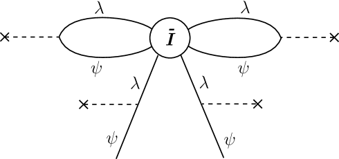
Figure 2: One-instanton contribution in the SU(2) model with one flavor.

In the ${\cal N}=2$ theory with no matter hypermultiplets the instanton has four gluino and four quark zero modes attached to it (Fig. 3). One can neutralize them all by virtue of the insertion of $\langle\bar{\Phi}\rangle$. That is why in the model at hand two, three, etc. instantons manifest themselves essentially in the same way as one. None contributes to the superpotential. Rather, they generate (4.61) – the integral $\int{\rm d}^{2}\theta\,W^{2}f(\Phi^{2})$ does not vanish on purely bosonic fields.

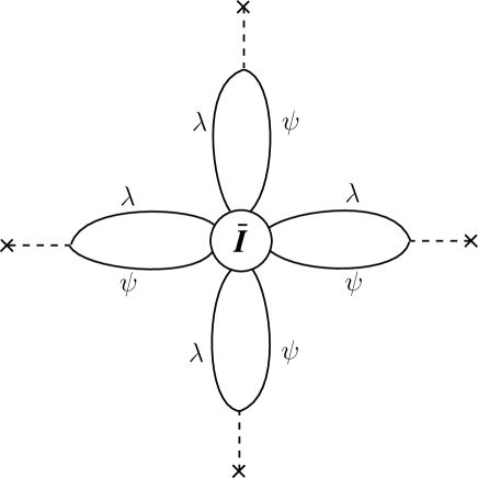
Figure 3: One-instanton contribution in the ${\cal N}=2$ theory (with no matter hypermultiplets).

The issue of one instanton vs. many was briefly touched in Sec. 4.1.5, in connection with the NSVZ $\beta$ function. In the models where the one-instanton results are exact, this $\beta$ function is exact not only perturbatively, but at the nonperturbative level too. On the other hand, in those models where the summation of the multi-instantons is needed, the NSVZ $\beta$ function ceases to be exact at the nonperturbative level. The function $f$ in Eq. (4.64) can be considered as a generalized (inverse) coupling constant. Just this function $f(\Phi^{2})$ was the central object of the Seiberg-Witten analysis based on holomorphy and duality. This novel approach provides a wealth of breakthrough insights regarding the nonperturbative SUSY gauge dynamics [95]. This interesting topic is outside the scope of this review.

The only question to be raised in connection with instanton calculus is whether one can construct ${\cal N}=1$ rather than ${\cal N}=2$ theories with the similar properties – the Coulomb phase, the vanishing $R$ charge of the relevant moduli, and an infinite series for the generalized coupling constant saturated by multi-instantons.

A systematic search for ${\cal N}=1$ theories with the simple gauge group and the Coulomb phase everywhere on the moduli space was carried out in Ref. [104]. The necessary condition on the matter sector was shown to be

$$\sum_{i}T(R_{i})=T_{G}\,,$$ (4.66)

where the sum runs over all matter fields. Note that the basic ${\cal N}=2$ model considered by Seiberg and Witten does obey this condition, automatically, since the matter field is in the adjoint representation. The number of models satisfying Eq. (4.66) is limited. One has to examine all of them in order to determine whether the pattern of the gauge symmetry breaking is indeed such that one is left with the unbroken U(1) irrespective of the values of the moduli. A general solution turns out to be unique – the SO($N$) models with $N-2$ vector matter fields (exceptional solutions exist also for SU(6) and Sp(6)). The conserved $R$ current in this model has the form

$$\lambda^{a}_{\alpha}\bar{\lambda}^{a}_{\dot{\alpha}}-\sum_{i=1}^{N-2}\psi^{i}_{\alpha}\bar{\psi}^{i}_{\dot{\alpha}}\,,$$

so the $R$ charge of $\psi^{\prime}s$ is $-1$, and the $R$ charge of the matter superfields vanishes. The generalized inverse coupling constant has the form similar to (4.64). The series can be summed up to produce a hyperelliptic curve, much in the same way as in the Seiberg-Witten solution of the ${\cal N}=2$ model.

5 Spontaneous Supersymmetry Breaking in Weak Coupling

In this and subsequent sections we will review what is known today regarding the dynamical supersymmetry breaking. The material covered in the previous part can be viewed an extended introduction to this critically important topic, which, in a sense, is the raison d’etre of multiple SUSY-based theoretical constructions. The spontaneous SUSY breaking can be realized by virtue of tree-level mechanisms discovered in the early 1970’s and described in text-books, and by virtue of nonperturbative mechanisms which are divided, in turn, in two classes – weak coupling and strong coupling mechanisms. There is no clear-cut boundary between the classes since some of the mechanisms under discussion in the current literature combine elements inherent to both classes. Some of the nonperturbative mechanisms were discovered in the 1980’s, others present a relatively recent development, dating back to Seiberg’s results of 1993/94. Finally, certain ideas are still controversial, and not all implications for the dynamical SUSY breaking are clear at the moment. The most notable example of this type is the chirally symmetric vacuum in SUSY gluodynamics [56]. If this vacuum indeed exists (we hasten to add that the final confirmation is still pending) then this would have a drastic impact on many conclusions regarding the dynamical SUSY breaking. Theories with no supersymmetric vacuum of the “old” type could develop one, of the Kovner-Shifman type, in the domain of strong coupling. This is especially transparent, for instance, in the one-generation SU(5) model (Sec. 6.1). Since the situation with the chirally symmetric vacuum is not yet settled, we will discuss the known mechanisms of the dynamical SUSY breaking forgetting for a while about its possible existence. Comments on the possible role of the Kovner-Shifman vacuum are collected at the very end (Sec. 7); a few marginal remarks are scattered in Secs. 5.5 and 6.1.

Many models exhibiting the dynamical SUSY breaking reduce in the low-energy limit to an effective theory of light degrees of freedom in which one of the known tree-level mechanisms acts. Therefore, to begin with, we briefly review them.

5.1 Traditional tree mechanisms (brief look at the old guide book)

Before submerging into nonperturbative dynamics it seems instructive to outline the conventional tree-level mechanisms leading to the spontaneous SUSY breaking. Our task here is to refresh memory and to emphasize common features and distinctions with the dynamical mechanisms.

Two such mechanisms are familiar for a long time. The first one, usually referred to as the O’Raifeartaigh, or $F$ term mechanism [105], works due to a “conflict of interests” between $F$ terms of various matter fields belonging to the matter sector. The necessary and sufficient condition for the existence of the SUSY vacuum is the vanishing of all $F$ terms. In the O’Raifeartaigh approach, the superpotential is arranged in such a way that it is impossible to make all $F$ terms vanish simultaneously. One needs minimally three matter fields in order to realize the phenomenon in the renormalized models with the polynomial superpotentials. With one or two matter fields and the polynomial superpotential the supersymmetric vacuum solution is always possible. With three superfields and the generic superpotential, supersymmetric solution exists too; it ceases to exist for some degenerate superpotentials.

Consider the superpotential

$${\cal W}(\Phi_{1},\Phi_{2},\Phi_{3})=\lambda_{1}\Phi_{1}(\Phi_{3}^{2}-M^{2})+\mu\Phi_{2}\Phi_{3}\,.$$ (5.1)

Then

$$\bar{F}_{i}=-\frac{\partial{\cal W}}{\partial\Phi_{i}}=\left\{\begin{array}[]{l}\lambda_{1}(\phi^{2}_{3}-M^{2})\,,\,\,\,~{}~{}~{}~{}~{}~{}i=1\,,\\[2.84544pt] \mu\phi_{3}\,,\qquad~{}~{}~{}~{}~{}~{}~{}~{}~{}~{}~{}~{}~{}i=2\,,\\[2.84544pt] 2\lambda_{1}\phi_{1}\phi_{3}+\mu\phi_{2}\,,\,\,\,\,~{}~{}~{}i=3\,.\end{array}\right.$$ (5.2)

The vanishing of the second line implies that $\phi_{3}=0$, then the first line cannot vanish. There is no solution with $F_{1}=F_{2}=F_{3}=0$ – supersymmetry is spontaneously broken.

What is the actual minimal energy configuration? It depends on the ratio $\lambda_{1}M/\mu$. For instance, at $M^{2}<\mu^{2}/(2\lambda_{1}^{2})$, the minimum of the scalar potential occurs at $\phi_{2}=\phi_{3}=0$. The value of $\phi_{1}$ can be arbitrary: an indefinite equilibrium takes place at the tree level. (The loop corrections to the Kähler potential lift this degeneracy and lock the vacuum at $\phi_{1}=0$.) Then $F_{2}=F_{3}=0$, and the vacuum energy density is, obviously, ${\cal E}=|F_{1}|^{2}=\lambda_{1}^{2}M^{4}$.

Since $F_{1}\neq 0$ the corresponding fermion is Goldstino, $m_{\psi_{1}}=0$. It is not difficult to calculate the masses of other particles. Assume that the vacuum expectation value (VEV) of the field $\phi_{1}$ vanishes. Then the fluctuations of $\phi_{1}$ remain massless (and degenerate with $\psi_{1}$). The Weyl field $\psi_{2}$ and the quanta of $\phi_{2}$ are also degenerate; their common mass is $\mu$. At the same time, the fields from $\Phi_{3}$ split: the Weyl spinor $\psi_{3}$ has the mass $\mu$, while

$$m_{a}^{2}=\mu^{2}-2\lambda_{1}^{2}M^{2}\,,\,\,\,m_{b}^{2}=\mu^{2}+2\lambda_{1}^{2}M^{2}\,,$$ (5.3)

where

$$\phi_{3}\equiv\frac{1}{\sqrt{2}}(a+ib)\,.$$

Note that in spite of the splitting

$$m_{a}^{2}+m_{b}^{2}-2m_{\psi_{3}}^{2}=0\,,$$ (5.4)

as if there is no SUSY breaking. Equation (5.4) is a particular example of the general supertrace relation [106]

$$\mbox{Str}\,{\cal M}^{2}\equiv\sum_{J}(-1)^{2J}(2J+1)m_{J}^{2}=0\,,$$ (5.5)

where Str stands for supertrace, ${\cal M}^{2}$ is the mass squared matrix of the real fields in the supermultiplet; the subscript $J$ marks the spin of the particle. Equation (5.5) is valid only at the tree level – quantum corrections arising due to SUSY breaking do modify it. It also gets modified in the theories where (a part of) SUSY breaking occurs due to the Fayet-Iliopoulos mechanism, speaking of which we must turn to a rather narrow subclass of theories that possess a U(1) gauge symmetry.

The Fayet-Iliopoulos mechanism [107], which is also called the $D$ term SUSY breaking, applies in the models where the gauge sector includes an U(1) subgroup. The simplest and most transparent example is SQED (Sec. 2.3.1).

In order to launch the spontaneous SUSY breaking a (Lorentz scalar) field transforming nontrivially under supersymmetry must acquire a VEV. In the O’Raifeartaigh mechanism this role was played by an $F$ component of a chiral superfield. The $D$ component of the vector superfields is also non-invariant under SUSY transformations. If it develops a non-vanishing VEV, supersymmetry is spontaneously broken too. In order to make $D$ develop a VEV, a $\xi$ term, which is called the Fayet-Iliopoulos term, must be added in the action, see Eq. (2.28).

Although the Fayet-Iliopoulos term literally does not exist in the non-Abelian gauge theories an analog of the phenomenon does exist: the kinetic part of the action $\bar{Q}e^{V}Q$ determines the form of the $D$ term in the Higgs phase. The conflict between the requirements of vanishing of the $D$ and $F$ terms may lead the spontaneous SUSY breaking.

Returning to SQED, Eq. (2.31) shows that with the massive matter ($m\neq 0$) the zero vacuum energy is not attainable. Indeed, the mass term requires $S$ and $T$ to vanish in the vacuum, while the $D$ term in the potential requires $|T|^{2}=|S|^{2}+\xi$. If $\xi\neq 0$ both conditions cannot be met simultaneously.

If $\xi>m^{2}/e^{2}$ the minimal energy is achieved at

$$S^{+}S=0\,,\,\,\,T^{+}T=\xi-\frac{m^{2}}{e^{2}}\,.$$

The minimal energy

$${\cal E}=m^{2}\left(\xi-\frac{m^{2}}{2e^{2}}\right)$$

is positive, so that SUSY is spontaneously broken. In addition, the gauge U(1) is broken too. The phase of $T$ is eaten up in the Higgs mechanism, the photon becomes massive, $m_{\gamma}=e\sqrt{\xi-(m^{2}/e^{2})}$. A linear combination of the photino and $\psi_{t}$ is the Goldstino; it remains massless. Another linear combination, as well as the scalar and spinor fields from $S$ are massive.

If $0<\xi<m^{2}/e^{2}$ the scalar fields develop no VEVs, the vacuum configuration corresponds to

$$S^{+}S=T^{+}T=0\,,$$

while the vacuum energy is ${\cal E}=e^{2}\xi^{2}/2$. The gauge U(1) remains unbroken: the photon is massless, while the photino assumes the role the Goldstino. The fermion part of the matter sector does not feel the broken supersymmetry (at the tree level),

$$m_{\psi_{s}}=m_{\psi_{t}}=m\,,$$

while the boson part does

$$m_{s}^{2}=m^{2}+e^{2}\xi\,,\,\,\,m_{t}^{2}=m^{2}-e^{2}\xi\,.$$

5.2 Dynamical mechanisms: preliminaries

In the majority of examples discussed so far the gauge symmetry is typically spontaneously broken [5, 22, 23] (it would be more exact to say that it is realized in the Higgs regime). Instantons are instrumental in this phenomenon, which provides a number of evident advantages; the weak coupling regime and calculability of the nonperturbative effects are the most important ones. The phenomenon is quite universal. In almost any model with matter there are classically flat directions, vacuum valleys, and together with them there arises a potential possibility for destabilization of the unbroken vacuum at the origin (vanishing values of the moduli). Roughly speaking, the theory is pushed away from the origin by instantons.

Our main subject here is the dynamical SUSY breaking. Among a vast variety of models with the spontaneously broken gauge symmetry we will choose those where SUSY is broken too. This will provide us with calculable scenarios of dynamical SUSY breaking. In a few instances it was argued that SUSY is broken in the strong coupling regime, where direct calculations are impossible. One then relies on indirect arguments. We will discuss such scenarios too. Our strategy is pragmatic: starting from simpler scenarios we will be moving towards more complicated ones.

The very same aspect – weak vs. strong coupling SUSY breaking – can be viewed from a slightly different angle. Let us discuss a generic hierarchy of scales inherent to a typical supersymmetric theory with matter. First, there exists an intrinsic scale $\Lambda_{g}$ of the underlying gauge theory . The scale of the dynamical SUSY breaking $\Lambda_{\rm dsb}$ can be of order $\Lambda_{g}$ or much lower than $\Lambda_{g}$. In the latter case when one descends below $\Lambda_{g}$ all gauge degrees of freedom can be integrated out, and one is left with the dynamics of the would-be moduli. This effective low-energy dynamics can be described by generalized Wess-Zumino models which can be studied relatively easily. SUSY is dynamically broken if a generalized O’Raifeartaigh mechanism takes place.

The most common scenario of this type is as follows. Assume that in a model with chiral matter (so that Witten’s index vanishes) there are classically flat directions in the limit of vanishing Yukawa terms. If instantons generate a repulsive superpotential, if the model can be completely stabilized by the Yukawa terms, so that the exits from all valleys are blocked (the run-away vacua totally excluded), if all Yukawa couplings are small (dimensionless couplings $\ll 1$, dimensional $\ll\Lambda_{g}$) – if all these “ifs” are satisfied – then dynamical SUSY breaking will most certainly occur in the weak coupling regime.

There is an alternative version of the weak coupling scenario. In some models (e.g. Sec. 5.5) the original gauge group is only partly broken, and the superpotential for the moduli is generated by the gluino condensation in the unbroken subgroup, rather than through the one-instanton mechanism. These models are still calculable because (i) so is the gluino condensate, and (ii) the SUSY breaking is due to dynamics of the moduli fields at a low-energy scale $\Lambda_{\rm dsb}\ll\Lambda_{g}$, where all (strongly interacting) degrees of freedom associated with the unbroken subgroup can be integrated out.

On the other hand, if $\Lambda_{\rm dsb}\sim\Lambda_{g}$, relevant dynamics is that of the strong coupling regime. Here one can hope, at best, to establish the very fact of SUSY breaking using global symmetry arguments and/or ’t Hooft matching [108].

Two criteria are known in the literature [22, 109], each of which guarantees spontaneous SUSY breaking.

Criterion 1. Suppose that the Yukawa terms in the superpotential introduced for the sake of stabilization at large values of moduli do not contain some matter superfield $Q$, or a linear combination of several superfields. In this case the gluino condensate is an order parameter – a non-zero VEV of the gluino density, $\langle\mbox{Tr}\,\lambda^{2}\rangle\neq 0$, implies the spontaneous SUSY breaking. This statement is quite transparent. Assume some superfield $Q$ enter in the original action only through its kinetic term $\left.\bar{Q}e^{V}Q\right|_{D}$. In this case the anomalous Konishi relation [52] takes the form (Sec. 2.8)

$$\bar{D}^{2}(\bar{Q}e^{V}Q)\propto\,{\rm Tr}\,W^{2}\,.$$ (5.6)

Then the vacuum expectation value of Tr$\,W^{2}$ is equivalent to the vacuum expectation value of the operator $\bar{D}^{2}(\bar{Q}e^{V}Q)$. Taking the spinor derivative is equivalent to the (anti)commutation with the supercharge. Hence in the theories with the unbroken SUSY no VEV’s of full superderivatives can develop. Thus, for $\langle\mbox{Tr}\,\lambda^{2}\rangle\neq 0$ we observe a contradiction.

Criterion 2. Suppose that in a theory under consideration the vacuum valleys are completely absent, i.e. they are non-existent from the very beginning (as in the SU(5) theory with one quintet and one (anti)decuplet), or the vacuum degeneracy is fully lifted by the tree-level superpotential. If in such a theory some exact continuous global symmetry is spontaneously broken, so is SUSY.

A sketch of the proof [110] is as follows. If a continuous global invariance is spontaneously broken, there is a massless Goldstone boson, call it $\pi$. Suppose, SUSY is unbroken. Then $\pi$ must be accompanied by massless superpartners, in particular, a scalar particle $\sigma$ with spin 0. Since the field $\pi$, being the Goldstone boson, appears in the Lagrangian with a zero potential, the potential for $\sigma$ must vanish too, and, as a consequence, the vacuum expectation value $\langle\sigma\rangle$ is not fixed. In other words, $\sigma+i\pi$ is a modulus, which can be varied arbitrarily, corresponding to a continuously degenerate vacuum manifold . This contradicts, however, the initial assumption of no flat directions. The only possibility of getting rid of the contradiction is to conclude that SUSY is spontaneously broken.

The above two criteria are not completely independent. In fact, if some superfield does not enter into the classical superpotential (Criterion 1), then there exists an axial $R$ current – a linear combination of the matter current and gluino current – which is strictly conserved. Further, the operator Tr$\,\lambda^{2}$ is obviously noninvariant with respect to the transformations generated by this current. Therefore, the gluino condensation, $\langle\mbox{Tr}\,\lambda^{2}\rangle\neq 0$, automatically implies spontaneous breaking of the corresponding axial symmetry.

5.3 Dynamical SUSY breaking in the 3-2 model

The simplest model where dynamical SUSY breaking takes place is the 3-2 model of Affleck, Dine and Seiberg [22]. This chiral model was discussed at length in Sec. 2.5.2 where a description of the classical moduli space (its complex dimension is three) was given. The Kähler potential on the moduli space was calculated.

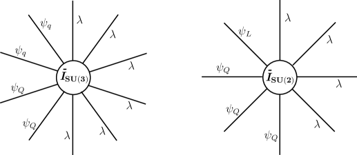
Figure 4: The 3-2 model: the zero mode structure in the field of the anti-instanton in the gauge groups SU(3) and SU(2), respectively. $\lambda$ denotes the SU(3) gluinos in the first case and SU(2) gluinos in the second.

Two chiral invariants, $I_{1}$ and $I_{2}$, where $I_{1,2}$ were defined in Eq. (2.60), are cubic; a combination thereof can be used as a (renormalizable) tree-level superpotential. Its purpose is to block the valleys and spare us of the run-away vacua. Note that the kinetic part possesses a global flavor SU(2) symmetry: $\bar{u}$ and $\bar{d}$ fields can be freely rotated into one another. In addition to this global SU(2), the theory has two strictly conserved U(1) currents. One of them is that of the hypercharge ($=2\times$the mean electric charge in the weak SU(2) multiplet). In SM this current would be coupled to the U(1) gauge boson, but since we remove the latter from the model, the corresponding symmetry is just a global U(1) invariance. The second U(1) is the anomaly-free $R$ current involving gluinos.

The fastest way of establishing the U(1) charges is through instantons themselves. The instanton in the SU(3) gauge group has six gluino zero modes, two $\psi_{Q}$ and two $\psi_{q}$. (A concise mnemonical formula is $\lambda^{6}\,\psi_{Q}^{2}\,\psi_{q}^{2}\,$, see Fig. 4. We will consistently use similar formulas below). The instanton in SU(2) has four gluino zero modes, three $\psi_{Q}$ and one $\psi_{L}$, i.e. $\lambda^{4}\,\psi_{Q}^{3}\,\psi_{L}$ for a shorthand. It is convenient to choose the conserved anomaly-free Konishi current in the form

$$\frac{1}{3}\bar{Q}^{f}Q_{f}-\frac{1}{3}\bar{q}^{\bar{f}}q_{\bar{f}}-\bar{L}^{f}L_{f}\,,$$

where the summation over the SU(3) indices in the first two terms is implicit. As for the $R$ current, we conveniently define it in such a way that $R(L)=0$. Then, $R(\psi_{L})=-1$ and $R(\psi_{Q})=-1$ too (the latter is immediately seen from the $\lambda^{4}\psi_{Q}^{3}\psi_{L}$ structure of the SU(2) instanton). Hence, $R(Q)=0$. From the $\lambda^{6}\psi_{Q}^{2}\psi_{q}^{2}$ structure of the SU(3) instanton we conclude that $R(\psi_{q})=-2$ which entails, in turn, $R(q)=-1$. The Konishi and $R$ charges of the superfields and invariants $I_{\bar{f}}$ and $J$ are summarized in Table 5

By an appropriate global SU(2) rotation one can always arrange that the tree-level superpotential has the form

$${\cal W}_{\rm tree}=hQ^{\alpha f}\bar{d}_{\alpha}L^{g}\varepsilon_{fg}=hI_{2}\,,$$ (5.7)

so that $I_{1}$ does not appear in the superpotential. This means, in turn, that $\bar{u}_{\alpha}$ does not appear in ${\cal W}$; we will make use of this fact later.

Field	$Q$	$q$	$L$	$I_{\bar{f}}$	$J$
U(1)K	1/3	$-1/3$	$-1$	$-1$	0
U(1)R	0	$-1$	0	$-1$	$-2$

Table 5: The U(1) charges of the superfields $Q$, $q$, $L$ and invariants $I_{\bar{f}}$ and $J$ defined in Eqs. (2.60), (2.61) in the 3-2 model.

As in MSSM it will be assumed that the SU(3) gauge coupling $g_{3}$ is much larger than the SU(2) gauge coupling $g_{2}$, and, in addition,

$$h\ll g_{2}\ll g_{3}.$$ (5.8)

The smallness of $h$ will automatically ensure that $\Lambda_{\rm dsb}\ll\Lambda_{3,2}$ where $\Lambda_{3,2}$ are the scale parameters of SU(3) and SU(2), respectively.

A generic point on the moduli space corresponds to complete breaking of all gauge symmetries; the theory is totally Higgsed. It is not difficult to check that the tree-level superpotential (5.7) locks all exits from the valleys – escape to large values of the moduli is impossible since there the energy is positive rather than vanishing. (This exercise is left for the reader.)

Now we switch on nonperturbative effects taking into account only instantons in the gauge SU(3) and neglecting the SU(2) instantons whose impact is much weaker because $g_{2}\ll g_{3}$. What is the general constraint on the instanton-induced superpotential? First, it cannot depend on $I_{\bar{f}}$ since $I_{\bar{f}}$ is not singlet with respect to global SU(2), and it is impossible to built any singlet from $I_{\bar{f}}$. On the other hand, $J$ is singlet and its Konishi charge vanishes. Thus, it is a suitable candidate. Examining the $R$ charge of $J$ we conclude that the only possible superpotential has the form

$${\cal W}_{\rm inst}=\frac{2(\Lambda_{3})^{7}}{J}\,.$$ (5.9)

The factor 2 is singled out for convenience; the power of $\Lambda_{3}$ is established on dimensional grounds, it exactly matches the first coefficient of the $\beta$ function in the SU(3) model with two triplets and two anti-triplets.

Is the superpotential (5.9) actually generated by the SU(3) instanton? To answer this question it is not necessary to perform the calculation anew – the problem can be readily reduced to that of our reference model, SU(2) SQCD with one flavor (Sec. 4.3). Indeed, let us assume that $|\tau_{1}|\gg|\tau_{2}|$ in Eq. (2.62). Then the pattern of breaking of SU(3) is step-wise: first one breaks SU(3)$\to$SU(2) at a high scale, and then at a much lower scale SU(2) is broken down completely. Below the higher scale the fields $Q$ and $q$ with the SU(2) index $f=\bar{f}=1$ disappear – they are eaten up by five SU(3) gauge bosons  which become very heavy and, in their turn, also disappear from the light spectrum. We are left with the SU(2) theory with one flavor, $Q^{\alpha 2}\,,\,\,q_{\alpha\bar{2}}\,,\,\,\,\alpha=2,3$. In this corner of the moduli space the invariant $J$ becomes $J\to\tau_{1}^{2}\,Q^{\alpha 2}\,q_{\alpha\bar{2}}$ where the summation over $\alpha$ runs over $\alpha=2,3$. Then, confronting Eq. (5.9) with Eq. (4.36) we immediately conclude that the superpotential (5.9) is indeed generated, the relation between the scale parameter of SU(2) and $\Lambda_{3}$ being $\Lambda_{3}=(\tau_{1}^{2}\,\Lambda^{5}_{\rm one-fl})^{1/7}$.

The instanton-induced superpotential pushes the scalar fields away from the origin and launches the spontaneous breaking of SUSY in the weak coupling regime. To prove the dynamical SUSY breaking quickly, we can use Criterion 1 (Sec. 5.2), since $\bar{u}$ does not appear in ${\cal W}_{\rm tree}$. From the $\lambda^{6}\,\psi_{Q}^{2}\,\psi_{q}^{2}$ structure of the zero modes it is perfectly clear that the condensate of Tr$\,\lambda^{2}$ actually develops. (Two gluino zero modes are neutralized by the operator Tr$\,\lambda^{2}$ whose vacuum expectation value we calculate. The remaining four gluino zero modes are paired with $\psi_{q}$ and $\psi_{Q}$, as in Fig. 3.). The run-away vacuum is impossible. Since Tr$\,\lambda^{2}\neq 0$, supersymmetry is broken.

To obtain a more detailed information on the particle spectrum it is necessary to investigate the effective low-energy Wess-Zumino model for the moduli. One can either use the explicit parametrization of the moduli fields given in Eq. (2.62), with the canonic kinetic terms , or, instead, deal directly with the moduli $I_{\bar{f}}$, $\,J$. In the latter case the superpotential term is trivial, but the kinetic term acquires the Kähler potential ${\cal K}$. Both methods have their advantages and disadvantages; the second approach is more common, however. One of the reasons is that it automatically takes care of the global symmetry on the moduli space.

The total superpotential is

$${\cal W}={\cal W}_{\rm tree}+{\cal W}_{\rm inst}\,.$$ (5.10)

The subsequent procedure is standard: one minimizes the scalar potential $U$ obtained from the given superpotential and the Kähler potential presented in Eq. (2.69),

$$U=\left[G^{-1}\right]_{i\bar{j}}\frac{\partial{\cal W}}{\partial\phi_{i}}\,\frac{\partial\bar{\cal W}}{\partial\bar{\phi}_{\bar{j}}}$$ (5.11)

where

$$G^{i\bar{j}}=\frac{\partial^{2}\,{\cal K}}{\partial\phi_{i}\partial\bar{\phi}_{\bar{j}}}$$ (5.12)

is the Kähler metric, $G^{-1}$ is the inverse matrix, and $\phi_{1,2,3}$ are the lowest components of the moduli $I_{\bar{f}}$ and $J$.

Unlike the superpotential, which is exact both perturbatively and nonperturbatively, the Kähler metric is renormalized in higher loops. However, if the solution for the vacuum lies at large values of the moduli – which is the case, as we will see a posteriori, provided $h\ll 1$ – then all gauge bosons are heavy, the gauge coupling is small, and the corrections to ${\cal K}$ are negligible.

Minimizing $U$ one gets [22]:

$$(\tau_{1})_{\rm vac}\approx 1.29\,\frac{\Lambda_{3}}{h^{1/7}}\,,\,\,\,(\tau_{2})_{\rm vac}\approx 1.25\,\frac{\Lambda_{3}}{h^{1/7}}\,,\,\,\,{\cal E}\approx 3.59\,h^{10/7}\,\Lambda_{3}^{4}\,.$$ (5.13)

In the limit $h\to 0$ the parameters $\tau_{1}$ and $\tau_{2}$ tend to infinity, as was expected. This justifies the assertion of the weak coupling regime. The masses of the gauge bosons are $M\sim g\Lambda_{3}h^{-1/7}\to\infty$.

The (former) massless moduli either remain massless or become light particles. One Weyl fermion, Goldstino, is exactly massless. The role of Goldstino belongs to the electron, as can be seen either directly from the effective low-energy Lagrangian or indirectly, from the ’t Hooft matching.

The relevant anomalous triangle is that of three hypercharges. Remember, the hypercharge is not gauged in the model at hand, so that this is an “external” anomaly eligible for the ’t Hooft matching. The anomalous triangle does not vanish due to the fact that the positron was removed from the matter sector in passing from SM to the 3-2 model under consideration. In addition, we get a neutral fermion with mass $\approx 11.3h^{6/7}\Lambda_{3}$.

Among the scalar partners there is one strictly massless Goldstone boson, corresponding to the spontaneous breaking of the $R$ symmetry, and one charged and three neutral scalars with masses $\sim h^{6/7}\Lambda_{3}$.

The 3-2 model presents a standard pattern of the dynamical SUSY breaking in the weak coupling regime. Analyses of other models with the same dynamical behavior go in parallel.

5.4 SU(5) model with two generations

The analysis of this model at the classical level was carried out in Sec. 2.5.3 where an explicit parametrization of the $D$-flat directions was presented and the Kähler potential on the moduli space built. A few additional remarks are necessary in order to complete the treatment of the model. First of all, in accordance with the general strategy, the exits from the valleys must be locked by a tree-level superpotential term. If one limits oneself to renormalizable theories, this term can only contain the $M$ invariants cubic in the chiral superfields (see Eq. (2.70)). The chiral invariants of the $B$ type are quartic and, hence, if added, would ruin renormalizability. Of course, if one considers the model as an effective low-energy approximation, one is free to add the quartic invariants too. This has no qualitative impact on the dynamical picture, however, and we will not do that.

The most generic form of the tree-level cubic superpotential is

$${\cal W}_{\rm tree}=\lambda M_{1}\,.$$ (5.14)

It is always possible to rotate the fields to eliminate the $M_{2}$ term by using the global SU(2)_X invariance of the kinetic term. The superpotential (5.14) breaks SU(2)_X; the global SU(2)_V remains intact. Two anomaly-free axial U(1) symmetries also survive as exact symmetries of the model (see below). The coupling constant $\lambda$ is assumed to be small, $\lambda\ll 1$, to ensure calculability. Away from the origin of the moduli space the theory is in the Higgs regime. Generically, the gauge group SU(5) is completely broken. If we are far away from the origin, the gauge bosons are very heavy in the scale $\Lambda$, and the theory is weakly coupled. Small $\lambda$ will eventually lead to a vacuum located far away from the origin.

It is not difficult to check, using the explicit parametrization (2.72), that the tree-level term (5.14) locks all exits, so that the run-away vacuum is impossible. The next question one must address is whether instanton generates a superpotential pushing the theory away from the origin.

Again, as in 3-2 model, we first examine what can be said of the superpotential on general grounds. The instanton-induced superpotential term (in the limit $\lambda\to 0$) must involve both quintets and both (anti)decuplets, since there is one zero mode in each quintet and three zero modes in each decuplet (in addition to ten gluino zero modes, of course). Moreover, the above numbers of the zero modes imply that each $V$ superfield must be accompanied in the superpotential by three $X$ superfields. Second, the instanton-induced superpotential term must respect the global SU(2)${}_{X}\times$SU(2)_V invariance. This leaves us with a unique choice

$${\cal W}_{\rm inst}=\mbox{const}\,\times\frac{(\Lambda_{5})^{11}}{B_{\bar{g}f}B_{\bar{g}^{\prime}f^{\prime}}\epsilon^{\bar{g}\bar{g}^{\prime}}\epsilon^{ff^{\prime}}}\,,$$ (5.15)

where the power of $\Lambda$ in the numerator is established from dimensional counting, and the invariants $B_{\bar{g}f}$ are defined in Eq. (2.70). The expression in the denominator is nothing but the invariant $I_{2}$ defined in Eq. (2.74).

Equation (5.15) goes through additional checks. First, the power of $\Lambda$, eleven, matches the first coefficient of the $\beta$ function $3T_{G}-\sum_{i}T(R_{i})$. We remind that  $T(V)=1/2$ and $T(X)=3/2$. In SU(5) with two generations $3T_{G}-\sum_{i}T(R_{i})=11$.

The second test of Eq. (5.15) comes from counting the U(1) charges. As was mentioned, the model has two conserved anomaly-free U(1) currents. The Konishi current requires each $V$ to be accompanied by three $X$’s. We already know this. As for the $R$ charges, it is convenient to define the conserved $R$ current in such a way that $R(\psi_{X})=0$. Then, the $R$ charges of other fields are unambiguously fixed , they are collected in Table 6.

Field	$\psi_{X}$	$\psi_{V}$	$X$	$V$	$B$
$R\,\,\mbox{ charge}$	$0$	$-5$	$1$	$-4$	$-1$

Table 6: The $R$ charges in the SU(5) model with two generations.

With the given $R$ charges of the $X,V$ superfields the $R$ charge of ${\cal W}_{\rm inst}$ in Eq. (5.15) is two, in full accord with the exact $R$ invariance (in the limit $\lambda\to 0$).

What remains to be done is to verify, by a straightforward one-instanton calculation, that the dimensionless numerical constant in Eq. (5.15) does not vanish. There are no reasons for it to vanish, and it does not. Technically, one can exploit the very same trick we described in connection with the 3-2 model. Choose a corner of the moduli space corresponding to a two-stage breaking of the gauge group, SU(5) $\to$ SU(2) $\to$ nothing. If the scale of the first breaking is much higher than that of the second breaking, the elephant gauge bosons (i.e. those belonging to SU(5)/SU(2)) become very heavy and decouple, and the problem again reduces to the SU(2) model with one flavor, Sec. 4.3. We urge the reader to go through this calculation, and find the value of the numerical constant, this is a good exercise.

The resulting dynamical picture in the SU(5) model is very close to that in the 3-2 model of Sec. 5.3. The instanton-induced superpotential pushes the theory away from the origin of the valley. The tree-level superpotential does not allow the vacuum to run away. An equilibrium is achieved at large values of the chiral invariants, where the theory is in the weakly coupled (calculable) regime.

It is not difficult to check that the gluino condensate develops, much in the same way as in the 3-2 model. Since the superfield $X_{2}$ does not participate in the tree-level superpotential, Criterion 1 of Sec.  5.2 tells us that supersymmetry must be spontaneously broken. The SU(5) model under consideration is singled out from the zoo of others by its special feature: this is the only one in the class of models with the simple gauge group, $T_{G}>\sum_{i}T(R_{i})$, and purely chiral matter, which leads to the spontaneous breaking of SUSY in the weak coupling regime [111].

If one wants to know the light particle content of the theory in the SUSY breaking vacuum, one must work out an effective low-energy description. Again, this could be done either in terms of the explicit parametrization or by analyzing the effective Lagrangian for the moduli. The Kähler potential on the moduli space is presented in Eq. (2.76).

Analysis of the vacuum and light excitations was carried out in Ref. [112]. In the vacuum the values of the moduli scale as $v\sim\lambda^{-1/11}\Lambda$, while the vacuum energy density scales as ${\cal E}_{\rm vac}\sim\lambda^{18/11}\Lambda^{4}$. The model has four massless Goldstone bosons corresponding to the spontaneously broken global symmetries. Note that with the tree-level superpotential switched on, the global flavor symmetry is SU(2)${}_{X}\times$U(1)². It is spontaneously broken down to U(1). In addition, there are eight bosons with masses proportional to $\lambda v\sim\lambda^{10/11}\Lambda$.

5.5 The 4-1 model: SUSY breaking through gluino condensation

This model was treated in Refs. [32, 33]. The field content of the matter sector is easy to memorize: one starts from the SU(5) model with one generation and pretends that SU(5) is broken down to SU(4)$\times$U(1). Then

$$X_{\alpha\beta}\to A_{\alpha\beta}+Q_{\alpha}\,,\,\,\,V^{\beta}\to\bar{Q}^{\beta}+S\,.$$

In other words, we deal with $6+4+\bar{4}+1$. As we will see shortly, with this matter set the theory is not fully Higgsed, an unbroken SU(2) subgroup survives, it is in the strong coupling regime. Nevertheless, the light fields surviving at energies below $\Lambda_{2}$ are weakly coupled, their dynamics is described by a Wess-Zumino model which is fully calculable and ensures the spontaneous SUSY breaking.

As a warm-up exercise let us turn off the U(1) coupling and focus on the SU(4) theory (our intention is to take into account the U(1) later). In the SU(4) theory there are three moduli,

$$M=Q\bar{Q}\,,\,\,\,P=\mbox{Pf}(A)\,,\,\,\,\mbox{and}\,\,\,S\,.$$ (5.16)

We collected in Table 7 the $R$ charges of the elementary fields and the moduli.

$A$	$Q$	$\bar{Q}$	$S$	$M$	$P$
2	$-3$	$-1$	4	$-4$	4

Table 7: The $R$ charges in the 4-1 model.

A generic point from the vacuum valley corresponds to the $\mbox{SU(4)}\to\mbox{SU(2)}$ pattern of the gauge symmetry breaking. Thus, in the low-energy limit one deals with SU(2) SUSY gluodynamics, supplemented by three gauge-singlet moduli fields. Below the scale of SU(2) theory only the moduli survive; a nonperturbative superpotential for them is generated through the gluino condensation,

$${\cal W}\sim(\Lambda_{2})^{3}\sim\frac{(\Lambda_{4})^{5}}{\sqrt{MP}}\,,$$ (5.17)

where $\Lambda_{2,4}$ are the scale parameters of SU(2) and SU(4), respectively.

Now it is time to turn on the U(1) coupling. Then the $D$-flatness conditions with respect to U(1) eliminate one moduli field out of three. The remaining moduli are

$$I_{1}=MP\,\,\,\mbox{and}\,\,\,I_{2}=MS\,.$$

The superpotential (5.17) does not depend on $I_{2}$; it pushes $I_{1}$ towards infinity. To lock the valleys one can introduce a tree-level superpotential, much in the same way as in the 3-2 model. An appropriate choice of the superpotential is

$${\cal W}_{\rm tree}=hI_{2}\equiv hSM\,.$$ (5.18)

It is not difficult to show [32, 33] that adding $hSM$ one locks all $D$-flat directions, SU(4) and U(1), simultaneously, eliminating the possibility of the run-away behavior.

The resulting low-energy theory presents a close parallel to the 3-2 model and can be analyzed in the weak coupling regime. Basically, the only difference is the origin of the nonperturbative superpotential. In the 3-2 model it was provided by instanton, here by the gluino condensation. The gluino condensate is known exactly [58]. The procedure of the vacuum state searches is straightforward, albeit numerically tedious, as in the 3-2 model itself. We will not go into details here referring the reader to the original publications. The conclusion is that supersymmetry is dynamically broken. A non-supersymmetric vacuum is found at

$$v\sim\Lambda_{4}h^{-1/5}\gg\Lambda_{4}$$

where $v$ is the scale of the typical expectation value of the matter fields, so that all corrections (say, to the Kähler function) turn out to be small. The vacuum energy density scales as

$${\cal E}_{\rm vac}\sim h^{6/5}(\Lambda_{4})^{4}\,.$$

The 4-1 model is only the simplest representative of its class. It can be generalized in various directions. The basic idea – a nonperturbative superpotential through the gluino condensation in an unbroken subgroup, plus a cleverly chosen tree-level superpotential – persists. In particular, 2k-1 models ($k>2$) were considered in [32, 33].

5.6 A few words on other calculable models

Using the strategy outlined above one can construct more complex calculable models with the spontaneously broken SUSY. The models based on products of unitary groups, SU($N$)$\times$SU($M$), are listed in Table 8.

Model	N -2	N -(N$-$1)	N-(N$-$2)
Matter	$\{N,2\}+2\,\{\bar{N},1\}$ $+\{1,2\}$	$\{N,N-1\}$ $+(N-1)\,\{\bar{N},1\}$ $+N\{1,\overline{N-1}\}$}	$\{N,N-2\}$ $+(N-2)\,\{\bar{N},1\}$ $+N\,\{1,\overline{N-2}\}$
Comments, references	$N$ odd, at $N>5$ quartic superpotential required, [32]	Non-renormalizable ${\cal W}_{\rm tree}$, [113]	Via duality related to $N$-2 models, [113]

Table 8: The SU($N$)$\times$SU($M$) models, usually referred to as the N-M models.

Simplectic and some other subgroups were considered too (e.g. [32, 114, 115]). It is hardly necessary to dwell on these examples since, with a single exception, they do not go beyond the range of ideas that are already familiar. The interested reader may consult the original publications.

The exception mentioned above is the use of Seiberg’s duality [31]. Assume that we have a dual pair such that the “electric” theory is weakly coupled while the “magnetic” theory is strongly coupled. Assume that one can establish that under a certain choice of parameters the “electric” theory spontaneously breaks supersymmetry. Then, SUSY must be broken in the “magnetic” theory too, and one learns something about this noncalculable breaking from consideration in the weak coupling regime. The information is not too abundant, though, since the full mapping between the “electric” and “magnetic” theories is not known. The best-known problem belonging to this class is the N-(N–2) model analyzed along these lines in [113]. Its dual strongly coupled partner is the N-2 model.

Another issue worth mentioning is a device, dating back to the 1980’s [58], allowing one to convert “non-calculable” models into calculable. The main idea is as follows. Given a model where SUSY is broken in the strong coupling regime, one introduces in this model, additionally, non-chiral matter (i.e. a set of matter fields with mass terms that are assumed to be small). Such an expansion definitely does not change Witten’s index. The extra matter fields may result in the emergence of the $D$ flat directions. If they do, and if a repulsive superpotential is generated, supersymmetry may be spontaneously broken in the weak coupling regime. The best known example of this type [33, 116] is the SU(5) theory with one anti-decuplet, one quintet plus one or two extra $\{{\bf 5}+{\bf\bar{5}}\}$. One may call it a non-minimal one-generation SU(5) model (non-minimal, because of the extra nonchiral matter). If the mass term of the extra flavor is small, the corresponding dynamics turns out quite similar to that of the 3-2 model: the theory is fully Higgsed, instanton does generate a superpotential term repulsing the theory from the origin, the exits from the valleys are locked. When the mass terms are small, the vacuum lies far away from the origin. Everything is calculable.

When the mass terms of the non-chiral matter fields increase, the vacuum moves towards the origin of the valley, and the coupling constant becomes stronger. Eventually, when all mass terms become of order $\Lambda_{5}$, the calculability is lost. (One still can argue, following an indirect line of reasoning, based on Criterion 2 in Sec. 5.2 and holomorphy, that SUSY stays broken. But this is a different story.)

One last remark in conclusion of this mini-survey. A class of promising calculable models based on the novel idea – the ITIY nonchiral mechanism of the dynamical SUSY breaking – was engineered by Dimopoulos et al. [16]. The ITIY model per se is noncalculable, and is considered in Sec. 6. The modification necessary in order to make it calculable, sometimes called the plateau mechanism, logically belongs to the current section, but it would be hardly possible to consider it here, prior to the discussion of the ITIY model. Therefore, we postpone a “get acquainted with the plateau mechanism” part till Sec. 6.3.

6 Spontaneous Supersymmetry Breaking in
Strong Coupling

6.1 SU(5) model with one generation

This is the simplest model where the dynamical SUSY breaking may occur, as was understood shortly after the search began [21, 20]. In fact, this is the simplest simple-gauge-group model with the nonchiral matter. It is truly strongly coupled, the only relevant parameter is $\Lambda$, no small parameters exist, and if SUSY is broken, the scale of the breaking has to be $\sim\Lambda$.

We are already familiar with many features of this model. It has no flat directions, no superpotential is possible, and it possesses two conserved U(1) currents – the Konishi current and the $R$ current. The corresponding charges of the matter fields are

$$Q_{K}(X)=-1,\,\,\,Q_{K}(V)=3\,;\qquad R(X)=1\,,\,\,\,R(V)=-9\,,$$ (6.1)

where our convention regarding the $R$ charge of $\psi_{X}$ is $R(\psi_{X})=0$, the same as in the SU(5) model with two generations. The zero mode formula is $\lambda^{10}\,\psi_{X}^{3}\,\psi_{V}$.

Both criteria of the dynamical SUSY breaking formulated in Sec. 5.2 are applicable. Here is how it works.

(i) Gluino condensation

Following [20] (see also Sec. 4.2) one can consider the correlation function

$$\Pi(x,y,z)=\langle T(\lambda^{2}(x),\lambda^{2}(y),\sigma(z))\rangle\,,$$ (6.2)

where

$$\sigma=\left.\epsilon^{\alpha\beta\gamma\delta\rho}X_{\alpha\beta}X_{\gamma\delta}\,(V^{\kappa}X_{\kappa\chi}\lambda^{\chi}_{\psi}\lambda^{\psi}_{\rho})\,\right|_{\theta=0}\,,$$ (6.3)

and the Greek letters are used for the SU(5) gauge indices (the Lorentz indices of the gluino field are suppressed).

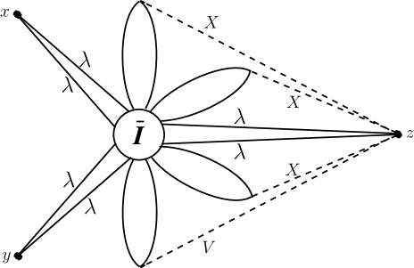
Figure 5: The instanton saturation of the correlation function (6.2) in the one-generation SU(5) model.

All operators in the correlation function $\Pi(x,y,z)$ are the lowest components of the chiral superfields. Then supersymmetry tells us that, if this correlation function does not vanish, it can only be an $x,y,z$ independent constant [3]. It goes without saying that $\Pi(x,y,z)$ vanishes in perturbation theory. The one-instanton contribution is non-vanishing, however, (see Fig. 5) and does, indeed, produce $\Pi\propto(\Lambda_{5})^{13}$ (The exponent 13 coincides with the first coefficient of the $\beta$ function.) If $x,y,z\ll\Lambda^{-1}$ one expects that the one-instanton contribution saturates $\Pi(x,y,z)$, so that the constant obtained in this way is reliable. If so, one can pass to the limit $x,y,z\to\infty$ and use the property of clusterization at large $x,y,z$ to argue that the gluino condensate develops , $\langle\lambda^{2}\rangle\neq 0$. Since the superpotential is absent, the gluino condensate is the order parameter for SUSY breaking. One concludes that supersymmetry is spontaneously broken [20].

(ii) Breaking of global symmetries

An alternative line of reasoning [21] is based on Criterion 2. Assume that neither of the two U(1) symmetries of the model (see Eq. (6.1)) is spontaneously broken. Then one has to match six ’t Hooft anomalous triangles [108]:

$$\mbox{Tr}\,Q_{R}=-26,~{}~{}~{}\,\,\,\mbox{Tr}\,Q_{K}=5,~{}~{}~{}~{}~{}\qquad\mbox{Tr}\,Q_{K}^{3}=125,$$

$$\mbox{Tr}\,Q_{R}^{3}=-4976,\,\,\,\mbox{Tr}\,Q_{R}Q_{K}^{2}=-450,\,\,\,\mbox{Tr}\,Q_{R}^{2}Q_{K}=1500\,.$$ (6.4)

Solutions of these matching conditions do exist [21] but they look rather awful. For instance, a minimal solution requires five massless composite Weyl fermions with the following assignment of the $\{Q_{K},Q_{R}\}$ charges:

$$(-5,26),\,\,\,(5,-20),\,\,\,(5,-24),\,\,\,(0,1),\,\,\,(0,-9)\,.$$

Since the solution is so complicated it is then natural to conclude (natural but not mandatory) that at least one of the axial symmetries is spontaneously broken, which, according to Criterion 2, would entail the spontaneous SUSY breaking. The spectrum of the theory must include at least several composite massless particles: the Goldstino, and one massless boson for each broken axial symmetry.

(iii) Adding nonchiral matter

Finally, the third alternative route providing an additional argument that SUSY is broken follows the strategy of [58] – adding nonchiral matter with a small mass term $m$ makes the theory more manageable by Higgsing (a part of) the gauge group and creating a theory whose dynamical behavior is simpler than that of the original one. The pattern of SUSY breaking/conservation can be established in this auxiliary model; then one can return back to the original model by sending $m\to\infty$. If no phase transition in $m$ happens en route one gets an idea of the vacuum structure of the original model.

This strategy was applied to the SU(5) model in [116] and [33], where one and two additional flavors, respectively, were introduced. For instance, with one extra flavor $(Q,\bar{Q})$ one arrives at a four-dimensional moduli space parametrized by four chiral invariants $XX\bar{Q}$, $Q\bar{Q}$, $XVQ$, and $V\bar{Q}$. A generic point from the vacuum valley corresponds to the breaking of the gauge SU(5) down to SU(2), with four color-singlet moduli. The low-energy theory for these moduli represents a generalized Wess-Zumino model. A nonperturbative superpotential is generated through the gluino condensation in the SU(2) theory. If the most general renormalizable tree-level superpotential is added, one arrives at a typical O’Raifeartaigh model of the spontaneous SUSY breaking [116]. Certainly, the limit $m\to\infty$ that returns us to the original theory and the strong coupling regime, cannot be achieved in a rigorous manner. The very fact of the SUSY breaking is a rigorous statement, however. Indeed, the gluino condensate $\langle\lambda\lambda\rangle$ depends on $m$ linearly . Therefore, if $\langle\lambda\lambda\rangle\neq 0$ at small $m$, it cannot vanish at large $m$.

Concluding this section let us note that the S0(10) model with a single spinor (i.e. 16-plet) representation is very similar to the one-generation SU(5). It is both chiral – no mass term is possible – and free from the internal anomalies. The model was treated along the same lines as the one-generation SU(5) model in the 1980’s [22]. Calculable deformations obtained by supplementing the original model by one nonchiral matter superfield in the representation 10 were considered by Murayama [116].

6.2 The Intriligator-Seiberg-Shenker model

The mechanism suggested by these authors [6] is the SU(2) gauge theory with a single matter superfield $Q$ in the representation 3/2, i.e. $Q_{\alpha\beta\gamma}$, symmetric in all three indices ($\alpha,\beta,\gamma=1,2$). This theory is chiral since no mass term is possible. Indeed, it is easy to see that the only quadratic invariant one could write $Q_{\alpha\beta\gamma}Q^{\alpha\beta\gamma}$ vanishes identically. Obviously, there are no cubic invariants. The first (and the only) nontrivial invariant is quartic,

$$u=Q_{\alpha\beta\gamma}Q^{\alpha\beta\rho}Q^{\tilde{\alpha}\tilde{\beta}\gamma}Q_{\tilde{\alpha}\tilde{\beta}\rho}\,.$$ (6.5)

Thus, a one-dimensional vacuum valley exists; it is parametrized by the modulus $u$. At the origin of the valley, $u=0$, the classical theory exhibits massless fields (the gauge bosons and gauginos). At $u\neq 0$ the gauge SU(2) is fully broken, the theory is fully Higgsed. If $u\gg\Lambda$, the gauge bosons are heavy, and the theory is weakly coupled.

The model possesses a single anomaly-free $R$ current , with the following $R$ charges:

$$R(\psi_{Q})=-\frac{2}{5}\,,\quad R(Q)=\frac{3}{5}\,.$$ (6.6)

The $R$ charge of $u$ is 12/5 while that of $\psi_{u}$ is 7/5. The $R$ charge conservation is spontaneously broken at $u\neq 0$.

Following [6] let us assume that a (nonrenormalizable) tree-level superpotential is added, ${\cal W}=u/M_{0}$, where $M_{0}$ is some ultraviolet parameter, $M_{0}\gg\Lambda$. This superpotential should be considered as a low-energy limit of some fundamental theory defined at the scale $M_{0}$. What exactly this fundamental theory is need not concern us here. The tree-level superpotential is treated in the first nontrivial order in $\Lambda/M_{0}$. It is not iterated – the iterations cannot be considered without the knowledge of the fundamental theory because of the nonrenormalizable nature of ${\cal W}=u/M_{0}$. Higher order effects in $\Lambda/M_{0}$ are discarded.

Classically the effective Lagrangian for the moduli field takes the form

$${\cal L}=\frac{1}{4}\int d^{4}\theta(\bar{u}u)^{1/4}+\left\{\frac{1}{2}\int d^{2}\theta\frac{u}{M_{0}}+\mbox{H.c.}\right\}\,.$$ (6.7)

It has a unique supersymmetric vacuum state at $u=0$. The tree-level superpotential pushes the theory towards the origin of the valley. The existence of the supersymmetric vacuum at $u=0$ is entirely due to the fact that the kinetic term for $u$ in Eq. (6.7) is singular at $u=0$.

While the kinetic term $(\bar{u}u)^{1/4}$ is definitely correct at large $u$, at small $u$ the singularity could be smoothed out provided that the theory at small $u$ is in the confining phase. Then, generally speaking, there are no reasons to expect that there are massless physical states, other than those described by the moduli field $u$, and, if so, one can expect the Kähler function to be regular at the origin,

$${\cal K}=(\bar{u}u)^{1/4}\,\longrightarrow\,{\cal K}=\Lambda^{-6}(\bar{u}u)+...\,,\>\qquad(|u|\ll\Lambda)\,.$$

Let us accept this assumption as a working hypothesis. Then the would-be supersymmetric vacuum at $u=0$ disappears. Indeed, at small $u$

$$F_{u}=\frac{\Lambda^{6}}{M_{0}}\,\,\,\mbox{and}\,\,\,{\cal E}=\frac{\Lambda^{6}}{M_{0}^{2}}\,.$$ (6.8)

The vacuum energy density is very small being measured in its natural units, ${\cal E}/\Lambda^{4}\ll 1$, but is definitely non-zero. Since at large $u$ the valley is locked and there is no supersymmetric solution either, one arrives at the conclusion of the spontaneous supersymmetry breaking in the model under consideration.

What are the arguments in favor of the hypothesis of the confining regime at small $u$ and no massless fields other than $u$ itself?

In essence, there is only one argument [6]: the ’t Hooft matching at $u=0$. At the origin of the valley the $R$ charge is conserved provided the small tree-level superpotential is switched off. There are two ’t Hooft triangles: Tr$\,Q_{R}$ and Tr$\,Q_{R}^{3}$. If the theory is in the confining regime, with no massless composites, both triangles must be matched by the contribution of $\psi_{u}$. And they do match! Indeed, it is easy to see that

$$\mbox{Tr}\,Q_{R}=\frac{7}{5}\,,\qquad\mbox{Tr}\,Q_{R}^{3}=\left(\frac{7}{5}\right)^{3}\,.$$

Since the $R$ charge of $\psi_{u}$ is 7/5, the matching is automatic.

Is this argument sufficiently conclusive in order to say that the theory is in the confining regime, and the Intriligator-Seiberg-Shenker mechanism works? Perhaps, not. In fact, one can give a rather strong argument pointing in the opposite direction.

Although the model at hand is asymptotically free, it is barely so. The first coefficient of the $\beta$ function is abnormally small, $\beta_{0}=6-5=1$. The second coefficient of the $\beta$ function is of a normal size and positive. So it is very likely that the $\beta$ function has a zero at a small value of $\alpha$, and the theory is conformal and relatively weakly coupled in the infrared, much in the same way as QCD with $N_{f}$ close to $11N_{c}/3$ [117, 118] or SQCD with $N_{f}$ slightly lower than $3N_{c}$, i.e. near the right edge of the conformal window [31]. The only distinction is that in the latter case, by sending $N_{c}\to\infty$, we can approach to the edge of the conformal window arbitrarily closely, so that the infrared fixed point of the $\beta$ function occurs at an arbitrarily small value of $\alpha$, and higher order effects are parametrically suppressed. In the Intriligator-Seiberg-Shenker model one has to rely on the numerical suppression of the higher order effects in $\gamma$. In order to give the reader the idea of the degree of suppression let us do this simple numerical exercise. The numerator of the NSVZ $\beta$ function in the model at hand is proportional to

$$3T_{G}-T(3/2)(1-\gamma(\alpha))=1+5\gamma(\alpha)\,,$$ (6.9)

where $\gamma(\alpha)$ is the anomalous dimension of the field $Q_{\alpha\beta\gamma}$. The infrared fixed point occurs at $\alpha_{*}$ such that

$$\gamma(\alpha_{*})=-\frac{1}{5}\,.$$ (6.10)

In the leading order

$$\gamma(\alpha)=-C_{2}(R)\frac{\alpha}{\pi}\,,$$ (6.11)

where

$$C_{2}(R)=T(R)\frac{\mbox{dim (adj) }}{\mbox{dim}(R)}=\frac{15}{4}\,\,\,\mbox{for}\,\,\,R=3/2\,.$$

The coefficient $C_{2}$ is rather large by itself; what is important, this numerical enhancement does not seem to propagate to higher order coefficients in $\gamma$. Combining Eqs. (6.10) and (6.11) one arrives at 

$$\frac{\alpha_{*}}{\pi}=\frac{4}{75}\,.$$ (6.12)

It seems rather unlikely that, with this small value of the critical coupling constant, the higher-order corrections are so abnormally large that they eliminate the infrared fixed point altogether.

What if the infrared fixed point exists in the weak coupling regime? Then, the infrared limit is conformal (the non-Abelian Coulomb phase). Needless to say that the ’t Hooft matching becomes uninformative: if the theory is in the non-Abelian Coulomb phase, the ’t Hooft triangles are trivially saturated by the unconfined gluino and quark fields themselves. Moreover, the singularity in the Kähler function need not be smoothed out, and the conclusion of the dynamical SUSY breaking becomes unsubstantiated. It is natural then to find a supersymmetric vacuum at $u=0$.

Everything seems self-consistent, except a single question: why then the two ’t Hooft triangles of the model, Tr$\,Q_{R}$ and Tr$\,Q_{R}^{3}$, are successfully saturated by the composite $\psi_{u}$? Can this matching be a mere coincidence?

We cannot be sure. It is worth adding, though, that at least one example of such a coincidental matching was found in a rather similar model [119]. The model consists of the SO($N$) gauge sector, plus a single matter (chiral) superfield in the (two-index symmetric traceless) tensor representation of SO($N$). The moduli fields of this model are known to saturate the ’t Hooft triangles corresponding to all unbroken global axial symmetries at the origin of the moduli space. One would then naturally expect to find the confining phase at the origin. At the same time, in Ref. [119] it was argued that the origin of the moduli space belongs to the non-Abelian Coulomb phase rather than to the confining phase, and the above matching by the moduli fermions is coincidental. The essence of the argument is beyond the scope of this review. The interested reader is referred to [119].

In summary, the Intriligator-Seiberg-Shenker model was designed to provide a new mechanism of the dynamical SUSY breaking. It remains to be seen whether it actually does the job. Even if the original SU(2) model is in the infrared-conformal phase and preserves supersymmetry one can try to construct other, more complicated models based on the same idea which, hopefully, do not fall in the conformal window. A promising candidate of this type is an SU(7) model [120] with two anti-symmetric tensors, six (anti)fundamentals and an appropriate tree-level superpotential, believed to be $s$ confining.

6.3 The Intriligator-Thomas-Izawa-Yanagida model

The model is nonchiral, Witten’s index is two. Nevertheless, supersymmetry is dynamically broken, in a manner briefly discussed in Sec. 2.10. Here we explain in detail how the ITIY mechanism works.

The model [7] is a close relative of the SU(2) model considered in Sec.  4.4. The matter chiral superfields $Q^{\alpha}_{f}$ are four color doublets ($\alpha=1,2$ and $f=1,2,3,4$ are color and subflavor indices). In addition to the “quark” superfields $Q^{\alpha}_{f}$, six color-singlet chiral superfields $S^{fg}=-S^{gf}$ are introduced. Their interaction with $Q_{\alpha f}$ is due to the superpotential,

$${\cal W}=\frac{h}{2}\,S^{fg}\,Q^{\alpha}_{f}\,Q^{\beta}_{g}\,\epsilon_{\alpha\beta}\;.$$ (6.13)

The theory is globally invariant under the SU(4) rotations of the subflavors. It also has a conserved $R$ charge: $Q^{\alpha}_{f}$ is neutral while the $R$ charge of $S^{fg}$ is two.

Let us start from the case $h=0$ when the superpotential (6.13) is switched off and the singlet fields $S^{fg}$ are decoupled. This case is well studied [30], see also Sec. 4.4. The classical moduli space is spanned by the gauge invariants

$$M_{fg}=-M_{gf}=Q^{\alpha}_{f}Q^{\beta}_{g}\,\epsilon_{\alpha\beta}$$ (6.14)

The matrix $M_{fg}$ is antisymmetric in $f,g$, its six elements are subject to one classical constraint (4.43). Nonperturbative quantum corrections change the geometry of the moduli space, the constraint ${\rm Pf}(M)=0$ is replaced by ${\rm Pf}(M)=\Lambda^{4}_{\rm two-fl}$, so that the origin is excluded.

Let us now switch on the interactions (6.13). It is clear that the consideration of Sec. 4.4 remains valid, with the substitution $m^{fg}\to hS^{fg}$ (the lowest component of $S^{fg}$ is implied). Thus one gets,

$$\left\langle M_{fg}\right\rangle=-\frac{1}{16\pi^{2}h}\,\left[\frac{1}{S}\right]_{fg}\left\langle\mbox{Tr}\,W^{2}\right\rangle\;;~{}~{}~{}~{}~{}\left\langle\mbox{Tr}\,W^{2}\right\rangle={\rm const}\,h\,\sqrt{{\rm Pf}(S)}\,\Lambda^{2}_{\rm two-fl}\;.$$ (6.15)

Now the fields $S^{fg}$ are dynamical; to determine the vacuum state one has to take into consideration their $F$ terms,

$$\left\langle F_{S^{fg}}\right\rangle=\left\langle\frac{\partial}{\partial S^{fg}}\,{\cal W}\right\rangle=h\left\langle M_{fg}\right\rangle\;.$$ (6.16)

Since $\left\langle M_{fg}\right\rangle$ does not vanish, $\left\langle M_{fg}\right\rangle\sim h\Lambda^{2}$, this leads to a clear contradiction with the presumed supersymmetry of the vacuum state.

To get a clearer picture of the phenomenon (and, in particular, to answer the question how SUSY can be broken in the theory where Witten’s index does not vanish, $I_{W}=2$) let us add a small mass term to the fields $S$. To keep our presentation as transparent as possible we will assume that

$$S^{12}=S^{34}\equiv S,\,\,\,\mbox{all other components vanish.}$$

In fact, for any general set of $S^{fg}$ one can always perform a global SU(4) rotation to eliminate all components other than $S^{12}$ and $S^{34}$.

The part of the superpotential containing $S$ consists of the tree-level term $mS^{2}$, plus the nonperturbative term due to the gluino condensation ,

$${\cal W}_{S}=\frac{1}{2}\,m\,S^{2}\pm\mbox{const}\,h\,S\,\Lambda^{2}_{\rm two-fl}\,.$$ (6.17)

We find two supersymmetric vacua at

$$S=\pm\mbox{const}\,h\,m^{-1}\Lambda^{2}_{\rm two-fl}\,,$$ (6.18)

in full accord with Witten’s index. In the limit of small $m$, however, these supersymmetric vacua lie very far in the space of fields. Let us see what happens at a finite distance in the space of fields.

If $|S|\ll h\,m^{-1}\Lambda^{2}_{\rm two-fl}$, the vacuum energy density ${\cal E}$ is just a constant,

$${\cal E}=|F_{S}|^{2}=\mbox{const}\,h^{2}\Lambda^{4}\,.$$ (6.19)

We get a plateau, or indefinite equilibrium.

The equilibrium is destroyed by the perturbative corrections to the Kähler function [121]. Assume that $h^{-1}\Lambda\ll|S|\ll h\,m^{-1}\Lambda^{2}$. Then the renormalization of the kinetic term is weak; at one loop it is given by the following $Z$ factor

$$Z=1+C\,\frac{h^{2}}{16\pi^{2}}\ln\frac{M_{\rm UV}}{h\,|S|}\,,$$ (6.20)

where $C$ is a positive constant and $M_{\rm UV}$ is the ultraviolet cut off. Inclusion of this correction tilts the plateau,

$${\cal E}=|F_{S}|^{2}\,Z^{-1}=\mbox{const}^{2}\,h^{2}\,\Lambda^{4}\left(1+C\,\frac{h^{2}}{16\pi^{2}}\ln\frac{M_{\rm UV}}{h\,|S|}\right)^{-1}\,,$$ (6.21)

making the theory slide towards smaller values of $|S|$. A minimum (or minima) is achieved somewhere at $h\,|S|\lower 3.01385pt\hbox{$\;\stackrel{{\scriptstyle\textstyle<}}{{\sim}}\;$}\Lambda$. At $h\,|S|\sim\Lambda$ Eq. (6.21) becomes inapplicable, of course. Perturbation theory becomes useless for the calculation of the Kähler potential. One can show [122], however, that at $|S|\lower 3.01385pt\hbox{$\;\stackrel{{\scriptstyle\textstyle<}}{{\sim}}\;$}\Lambda$ noncalculable terms in the Kähler potential are suppressed by powers of $h$ and are negligible provided that $h\ll 1$. One gets a stable non-supersymmetric vacuum at $\langle S\rangle=0$. Besides the Goldstino, at $\langle S\rangle=0$ the theory exhibits five massless Goldstone bosons corresponding to the spontaneous breaking of the global SU(4) down to Sp(4). Of course, the analysis of Ref. [122] has nothing to say about the possibility of finding a still lower non-supersymmetric vacuum at $h\,|S|\sim\Lambda$. In this domain the Kähler potential is noncalculable.

For finite values of $m$ the non-supersymmetric vacua are quasistable because of the tunneling into the supersymmetric vacuum at $\langle S\rangle\propto 1/m$. In the limit $m\to 0$ the tunneling probability vanishes, and the non-supersymmetric vacuum becomes stable.

An elegant idea of how to make the ITIY mechanism fully calculable by stabilizing the theory on the plateau at sufficiently large values of $S$ was suggested in Ref. [16]. Assume that a part of the global SU(4) of the ITIY model is gauged. The original gauge SU(2) – call it strong – is thus supplemented by additional weaker gauge interactions, with the gauge coupling $\alpha_{a}$, such that $\Lambda_{a}\ll\Lambda$ (the subscript $a$ means additional). The particular pattern considered in [16] was SU(2)$\times$ SU(2) weak gauge group. Note that the Yukawa coupling $h$ is a free parameter, so that the ratio of $\alpha_{a}/h$ can be arbitrary.

Then the $Z$ factor of the gauge fields gets a contribution both, from the Yukawa interactions and the weak gauge interactions. If $\alpha_{a}\gg h$ the tilt of the plateau is reversed (since the signs of these two contributions are opposite), $|S|$ is pushed towards large rather than small values. This drive towards large values of $|S|$ eventually stops since the running of $\alpha_{a}$ makes this coupling constant smaller at large $|S|$ while $h$ gets larger. Sooner or later $h$ wins over $\alpha_{a}$. The theory can be stabilized at arbitrarily large values of $|S|$, where the $Z$ factor is calculable to the degree of precision we want.

As an additional bonus one finds that at large values of $|S|$ the supersymmetry breaking effects can be as small as we want. At first sight this conclusion seems rather paradoxical since ${\cal E}_{\rm vac}\sim h^{2}\Lambda^{4}$ and is seemingly $S$ independent. One should not forget, however, that the natural unit of energy is set by the gluino condensate, $\langle\lambda^{2}\rangle\sim S\Lambda^{2}\gg\Lambda^{3}$. Being measured in these natural units, the vacuum energy is very small,

$${\cal E}_{\rm vac}\sim S^{-2}\langle\lambda^{2}\rangle^{2}\,,$$

and the spitting between the glueball/glueballino masses is of order $S^{-2}\langle\lambda^{2}\rangle$. The ratio of the splitting to the masses themselves tends to zero as $S^{-2}$. The $S$ superfield acts as a phantom axion/dilaton – asymptotically massless and non-interacting – much in the same way as the invisible axion of QCD [123].

Concluding this section let us note that a straightforward generalization of the ITIY mechanism based on SU($N$) SQCD with $N$ quark flavors and $N^{2}+2$ gauge singlets was considered in Ref. [122].

7 Impact of the Chirally Symmetric Vacuum

The existence of $T_{G}$ distinct (but physically equivalent) chirally asymmetric vacuum states in SUSY gluodynamics is a well-established fact. We have already mentioned in passing, that a physically inequivalent chirally symmetric state at $\langle\lambda^{2}\rangle=0$, the Kovner-Shifman vacuum, is not ruled out; moreover, certain arguments make one believe [56] that chirally symmetric regime is attainable, the $\langle\lambda^{2}\rangle=0$ phase of SUSY gluodynamics exists. If this is indeed the case, and if this vacuum does not disappear in the presence of sufficiently light (or massless) matter, it would lead to absolutely drastic consequences in many mechanisms of the dynamical SUSY breaking: they will simply disappear.

Let us first briefly review the arguments in favor of the Kovner-Shifman vacuum. First, it is present in the Veneziano-Yankielowicz effective Lagrangian (see Sec. 2.9) which encodes information on the anomalous Ward identities in SUSY gluodynamics and is expected to properly reflect its vacuum structure. Second, the instanton calculations of the correlation function $\langle\lambda^{2}(x)\lambda^{2}(0)\rangle$ at small $x$, performed in the strong coupling theory and in the weak coupling theory (i.e. adding matter in SU(2) SUSY gluodynamics, Higgsing the theory, and then returning back by using holomorphy in the matter mass parameter) do not match each other (Secs. 4.2, 4.3). The first method yields a smaller value for the gluino condensate than the second one [13]. The mismatch is $\sqrt{4/5}$ for SU(2). The mismatch could be explained if one invokes a hypothesis of Amati et al. [43], according to which the strong coupling calculation of the correlation function $\langle\lambda^{2}(x)\lambda^{2}(0)\rangle$ in fact yields a result averaged over all vacuum states of the theory. If the $\langle\lambda^{2}\rangle=0$ vacuum exists, it would contaminate this correlation function, explaining in a natural way the 4/5 suppression factor compared to the calculation in the weak coupling regime. The evidence for the chirally symmetric state is admittedly circumstantial. In particular, as it was discussed in Sec. 4.2, the hypothesis of Amati et al.[43] is in contradiction with the strong coupling solution of the ${\cal N}=2$ gluodynamics softly broken to ${\cal N}=1$.

The Kovner-Shifman vacuum must give zero contribution to Witten’s index since the latter is fully saturated by the chirally symmetric vacua. If so, it is potentially unstable under various deformations. For instance, putting the system in a finite-size box lifts the vacuum energy density from zero [124]. This vacuum disappears in finite volume . This instability – the tendency to escape under seemingly “harmless” deformations – may explain why the Kovner-Shifman vacuum at $\langle\mbox{Tr}\lambda^{2}\rangle=0$ is not seen in Witten’s $D$-brane construction [125] . Perhaps, this is not surprising at all. Indeed, there is a good deal of extrapolation in this construction, against which the chirally asymmetric vacua are stable (they have no choice since they have to saturate Witten’s index) while the $\langle\mbox{Tr}\lambda^{2}\rangle=0$ vacuum need not be stable and may not survive the space-time distortions associated with the $D$-brane engineering. Neither it is seen in the Seiberg-Witten solution [95] of ${\cal N}=2$ SUSY gluodynamics slightly perturbed by a small mass term  of the matter field $m$Tr$\,\Phi^{2}$, ($m\ll\Lambda$). If at all, it can exist only at large values of $m$, i.e. $m\gg\Lambda$.

One may ask a question: “Are we aware of any other examples of supersymmetric theories where Witten’s index vanishes, and the supersymmetric vacuum appears/disappears under deformations of parameters that do not change the structure of the theory, e. g. variations of mass parameters or putting the theory in a box of size $L$ and considering the theory at large but finite $L$ instead of the limit $L\to\infty$?”

The answer is yes. Surprisingly, the simplest two-dimensional theory with the minimal supersymmetry, ${\cal N}=1$, is of this type. The model we keep in mind (to be referred to as the minimal model) is similar to that described in detail in Sec. 3.3, but simpler. Assume that instead of two chiral superfields we deal with one (i.e. omit $\phi_{2}$ and $\psi_{2}$ from Eqs. (3.22) and (3.23)). This cubic superpotential model has Witten’s index zero. This can be seen in many ways. Say, if the mass parameter $m^{2}$ in the superpotential is made negative, the equation $\partial{\cal W}/\partial\phi=0$ has no real solutions. Alternatively, one can consider the theory with positive $m^{2}$ in a finite box, of length $L$. If $\lambda L\ll 1$, it is legitimate to retain only the zero momentum modes discarding all others. Then one gets a quantum-mechanical system known to have vanishing Witten’s index [2].

The minimal model at positive (and large) values of $m^{2}$ has two physically equivalent vacua, at $\phi=\pm\sqrt{2}m/\lambda$. The vanishing of Witten’s index implies that if one of the vacua is “bosonic”, the other is “fermionic”.

Although Witten’s index in the minimal model does vanish, supersymmetry is not spontaneously broken, provided $m^{2}$ is large and positive, i.e. $m^{2}\gg\lambda^{2}$. The supersymmetric vacuum with the zero energy density exists. Indeed, one can show that $v^{2}=m^{2}/\lambda^{2}$ is the genuine dimensionless expansion parameter in the theory at hand (the expansion runs in powers of $1/v^{2}$). At large $v^{2}$ the theory is weakly coupled. Since there are no massless fields in the Lagrangian, (and they cannot appear as bound states in the weak coupling regime), there is no appropriate candidate to play the role of Goldstino, and, hence, SUSY must be realized linearly.

At large negative $m^{2}$ the field $\phi$ does not develop a vacuum expectation value. SUSY is broken. The $\psi$ field is massless, and is the Goldstino of the spontaneously broken SUSY. In fact, one can argue that the SUSY breaking takes place at positive but small values of $m^{2}$, $m^{2}\sim\lambda^{2}$. The classical potential for such values of parameters has an underdeveloped peak at $\phi=0$ plus two shallow minima at $\phi\sim\pm 1$. The quantum corrections are likely to completely smear this structure, leaving no physical states at zero energy. The switch from the unbroken to spontaneously broken SUSY occurs as a phase transition in the mass parameter.

This example teaches us that it is not unreasonable to think of the existence of the $\langle\lambda^{2}\rangle=0$ phase of SUSY gluodynamics, even if neither the $D$-brane perspective nor the Seiberg-Witten solution of ${\cal N}=2$ at small $m$ carry indications on such a solution. Assuming that it exists, one may ask what are its implications on the SUSY breaking mechanisms we discussed.

The mechanisms that are based on the weak coupling regime are least affected. Formally, it may well happen that, apart from the SUSY-breaking vacua at large values of fields, there exists a SUSY-conserving vacuum at small values. These vacua are well-separated in the space of fields. The SUSY-breaking vacua remain as quasistable. Under an appropriate choice of relevant parameters the barrier may be arbitrarily large, and if the theory initially finds itself in the SUSY-breaking vacuum, it will never leak to the SUSY-conserving one, for all practical purposes. It is worth noting that the possibility of SUSY-conserving vacua, separated by a large distance in the space of fields from the SUSY-breaking vacuum, where the theory actually resides, was incorporated from the very beginning in the plateau models of Ref. [16]. The possibility of existence of the SUSY-conserving vacua in the domain of strong coupling in the 3-2 model or the two-generation SU(5) model just puts them in the same class as the plateau models.

The most affected are the mechanisms based on the gluino condensation in the strong coupling regime, e.g. the one-generation SU(5) model or the ITIY model. For them, the Kovner-Shifman vacuum may be a fatal blow. The ISS mechanism and its derivatives are neutral. As far as we see it now, they are independent of this phenomenon, and remain intact.

8 Concluding Remarks

The instanton calculus proved to be a powerful tool in analyzing supersymmetric theories. In this review we focused mainly on formal aspects of the method and several applications.

Although the instanton calculus score an impressive list of results, still some conceptual issues remain unclear. Two points are most disturbing. First, the result obtained via instantons as a rule are of the topological nature: they do not depend on specific details. For example, in the one-flavor model the nonperturbative superpotential is totally determined by the zero-size instantons. Second, the VEV scale $v$ inherent to the instanton calculations in the Higgs phase has no direct physical meaning. It is clear that instanton results are an indirect reflection of physics at the monopole/sphaleron scale $v/g$. The whole story reminds a famous Anderson’s fairy tail where a soldier cooked a soup from an axe.

An example where the relation to the monopole scale is established is provided by ${\cal N}=2$ theories [95] where one and the same function determines both the scattering amplitudes in the infrared and the monopole/dyon spectrum. We believe that a similar relation exists in ${\cal N}=1$ theories. An important task is to reveal it.

Recommended Literature

Books

D. Bailin and A. Love, Supersymmetric Gauge Field Theory and String Theory (IOP Publishing, Bristol, 1994).

A brief introduction to supersymmetric instanton calculus is given in

Instantons in Gauge Theories, ed. M. Shifman, (World Scientific, Singapore, 1994), Chapter VII.

A brief survey of those aspects of supersymmetry which are most relevant to the recent developments can be found in

J. Lykken, Introduction to Supersymmetry, hep-th/9612114.

Reviews on SUSY instantons and instanton-based mechanisms of supersymmetrty breaking

D. Amati, K. Konishi, Y. Meurice, G. Rossi and G. Veneziano, Phys. Rep. 162 (1988) 557.

V.V. Khoze, M.P. Mattis and M.J. Slater, Nucl. Phys. , B536 (1998) 69.

L. Randall, in Proc. Int. Workshop Perspectives of Strong Coupling Gauge Theories, Nagoya, Japan, 1996, Eds. J. Nishimura and K. Kamawaki (World Scientific, Singapore, 1997), page 258 [hep-ph/9706474].

W. Skiba, Mod. Phys. Lett. A12 (1997) 737.

E. Poppitz, Int. J. Mod. Phys. A13 (1998) 3051.

S. Thomas, in Proc. Int. Workshop Perspectives of Strong Coupling Gauge Theories, Nagoya, Japan, 1996, Eds. J. Nishimura and K. Kamawaki (World Scientific, Singapore, 1997), page 272 [hep-th/9801007].

E. Poppitz and S. Trivedi, Dynamical Supersymmetry Breaking, hep-th/9803107 [Ann. Rev. Nucl. Part. Sci., to be published].

References

- [1] E. Witten, Nucl. Phys. B185 (1981) 513 [Reprinted in Supersymmetry, Ed. S. Ferrara (North Holland/World Scientific, Amsterdam – Singapore, 1987), Vol. 1, page 443].
- [2] E. Witten, Nucl. Phys. B202 (1982) 253 [Reprinted in Supersymmetry, Ed. S. Ferrara (North Holland/World Scientific, Amsterdam – Singapore, 1987), Vol. 1, page 490]; J. High Energy Phys. 9802:006, 1998 (see Appendix).
- [3] V.A. Novikov, M.A. Shifman, A.I. Vainshtein, and V.I. Zakharov Nucl. Phys. B229 (1983) 407 [Reprinted in Supersymmetry, Ed. S. Ferrara (North Holland/World Scientific, Amsterdam – Singapore, 1987), Vol. 1, page 606].
- [4] G.C. Rossi and G. Veneziano, Phys. Lett. B138 (1984) 195 [Reprinted in Supersymmetry, Ed. S. Ferrara (North Holland/World Scientific, Amsterdam – Singapore, 1987), Vol. 1, page 620].
- [5] I. Affleck, M. Dine, and N. Seiberg, Nucl. Phys. B241 (1984) 493.
- [6] K. Intriligator, N. Seiberg, and S.H. Shenker, Phys. Lett. B342 (1995) 152.
-
[7]
K. Intriligator and S. Thomas, Nucl. Phys. B473 (1996)
121;
K. Izawa and T. Yanagida, Prog. Theor. Phys. 95 (1996) 829. - [8] A.A. Belavin, A.M. Polyakov, A.S. Schwartz, and Yu.S. Tyupkin, Phys. Lett. B59 (1975) 85 [Reprinted in Instantons in Gauge Theories, Ed. M. Shifman (World Scientific, Singapore, 1994), page 22].
- [9] G. ’t Hooft, Phys. Rev. D14 (1976) 3432; (E) Phys. Rev. D18 (1978) 2199 [Reprinted in Instantons in Gauge Theories, Ed. M. Shifman (World Scientific, Singapore, 1994), page 70; note that in the reprinted version the numerical errors summarized in Erratum above are corrected.]
- [10] A. D’Adda and P. Di Vecchia, Phys. Lett. B73 (1978) 162 [Reprinted in Instantons in Gauge Theories, Ed. M. Shifman (World Scientific, Singapore, 1994), page 293].
- [11] V.A. Novikov, M.A. Shifman, A.I. Vainshtein, and V.I. Zakharov Nucl. Phys. B229 (1983) 381; Phys. Lett. B166 (1986) 329.
- [12] V.A. Novikov et al., Nucl. Phys. B229 (1983) 394 [Reprinted in Instantons in Gauge Theories, Ed. M. Shifman (World Scientific, Singapore, 1994), page 298].
- [13] V.A. Novikov, M.A. Shifman, A.I. Vainshtein, and V.I. Zakharov Nucl. Phys. B260 (1985) 157 [Reprinted in Instantons in Gauge Theories, Ed. M. Shifman (World Scientific, Singapore, 1994), page 311].
- [14] G. Veneziano, Phys. Lett. B128 (1983) 199.
-
[15]
T. Banks and E. Rabinovici,
Nucl. Phys. B160 (1979) 349;
E. Fradkin and S. Shenker, Phys. Rev. D19 (1979) 3682. - [16] S. Dimopoulos, G. Dvali, G. Guidice, and R. Ratazzi, Nucl. Phys. B510 (1997) 12.
- [17] R. Arnowitt and P. Nath, in Proceedings of Summer School Jorge Andre Swieca: Particles and Fields, Ed. O.J.P. Eboli and V.O. Rivelles (World Scientific, Singapore, 1994) [hep-ph/9309277]; G. Guidice and R. Rattazzi, Theories with Gauge Mediated Supersymmetry Breaking, hep-ph/9801271 [Phys. Rep., to be published].
- [18] I. Affleck, J. Harvey and E. Witten, Nucl. Phys. B206 (1982) 413.
- [19] V.A. Novikov et al., Nucl. Phys. B223 (1983) 445.
- [20] Y. Meurice and G. Veneziano, Phys. Lett. B141 (1984) 69.
- [21] I. Affleck, M. Dine, and N. Seiberg, Phys. Lett. B137 (1984) 187 [Reprinted in Supersymmetry, Ed. S. Ferrara (North Holland/World Scientific, Amsterdam – Singapore, 1987), Vol. 1, page 600]; Phys. Rev. Lett. 52 (1984) 1677.
- [22] I. Affleck, M. Dine, and N. Seiberg, Phys. Lett. B140 (1984) 59; Nucl. Phys. B256 (1985) 557.
- [23] A.I. Vainshtein, V.I. Zakharov, V.A. Novikov, and M.A. Shifman, Pis’ma ZhETF 39 (1984) 494 [JETP Lett. 39 (1984) 601].
- [24] I. Affleck, M. Dine, and N. Seiberg, Phys. Rev. Lett. 52 (1984) 1677.
-
[25]
J. Fuchs and M. Schmidt,
Z. Phys. C30 (1986) 161; J. Fuchs, Nucl. Phys. B272
(1986) 677;
V. Novikov, Yad. Fiz. 46 (1987) 656; 967 [Sov. J. Nucl. Phys., 46 (1987) 366; 554]. - [26] A. Yung, Nucl. Phys. B485 (1997) 38.
- [27] N. Dorey, V. Khoze, and M. Mattis, Phys. Rev. D54 (1996) 2921; D54 (1996) 7832; Nucl. Phys. B513 (1998) 681; N. Dorey, T. Hollowood, V. Khoze, and M. Mattis, Nucl. Phys. B519 (1998 ) 470.
- [28] V. Khoze, M. Mattis, and M. Slater, Nucl. Phys. B536 (1998) 69.
- [29] N. Seiberg, Phys. Lett. B206 (1988) 75.
- [30] N. Seiberg, Phys. Rev. D49 (1994) 6857.
- [31] N. Seiberg, Nucl. Phys. B435 (1995) 129.
- [32] M. Dine, A. Nelson, Y. Nir and Y. Shirman, Phys. Rev. D53 (1996) 2658.
- [33] E. Poppitz and S. Trivedi, Phys. Lett. B365 (1996) 125.
- [34] J. Bagger and J. Wess, Supersymmetry and Supergravity, (Princeton University Press, 1990).
- [35] B. Chibisov and M. Shifman, Phys. Rev. D56 (1997) 7990; (E) D58 (1998) 109901.
- [36] J. Wess and B. Zumino, Phys. Lett. B49 (1974) 52 [Reprinted in Supersymmetry, Ed. S. Ferrara, (North-Holland/World Scientific, Amsterdam – Singapore, 1987), Vol. 1, page 77].
- [37] Yu.A. Gol’fand and E.P. Likhtman, JETP. Lett. 13 (1971) 323 [Reprinted in Supersymmetry, Ed. S. Ferrara, (North-Holland/World Scientific, Amsterdam – Singapore, 1987), Vol. 1, page 7].
- [38] J. Wess and B. Zumino, Nucl. Phys. B70 (1974) 39.
- [39] F. Buccella, J.-P. Derendinger, C. Savoy, and S. Ferrara, Phys. Lett. B115 (1982) 375, and in Proc. Europhys. Study Conf. Unification of the Fundamental Particle Interactions II, Eds. J. Ellis and S. Ferrara (Plenum Press, New York, 1983), page 349.
- [40] T.R. Taylor, Phys. Lett. B125 (1983) 185; B128 (1983) 403.
- [41] M. Luty and W. Taylor, Phys. Rev. D53 (1996) 3399.
- [42] N. Hitchin, A. Karlhede, U. Lindström and M. Roček, Commun. Math. Phys. 108 (1987) 535.
- [43] D. Amati, K. Konishi, Y. Meurice, G. Rossi and G. Veneziano, Phys. Rep. 162 (1988) 557.
- [44] E. Witten, Phys. Lett. B117 (1982) 324 [Reprinted in Instantons in Gauge Theories, Ed. M. Shifman (World Scientific, Singapore, 1994), page 230].
- [45] J. Bagger, E. Poppitz and L. Randall, Nucl. Phys. B426 (1994) 3.
- [46] A. Vainshtein, V. Zakharov, and M. Shifman, Usp. Fiz. Nauk, 146 (1985) 683 [Sov. Phys. Uspekhi, 28 (1985) 709].
- [47] T. ter Veldhuis, Phys. Rev. D58 (1998) 015010; Unexpected symmetries in classical moduli spaces, hep-th/9811132.
-
[48]
J. Wess and B. Zumino, Phys. Lett. B49 (1974) 52;
J. Iliopoulos and B. Zumino, Nucl. Phys. B76 (1974) 310;
P. West, Nucl. Phys. B106 (1976) 219;
M. Grisaru, M. Roček, and W. Siegel, Nucl. Phys. B159 (1979) 429. -
[49]
A. Salam and J. Strathdee, Nucl. Phys. B87 (1975) 85;
P. Fayet, Nucl. Phys. B90 (1975) 104. - [50] S. Ferrara and B. Zumino, Nucl. Phys. B87 (1975) 207.
- [51] M. Grisaru, in Recent Developments in Gravitation (Cargése Lectures, 1978), Eds. M. Levy and S. Deser (Plenum Press, New York, 1979), page 577, and references therein.
-
[52]
T.E. Clark, O. Piguet, and K. Sibold, Nucl. Phys. B 159 (1979)
1;
K. Konishi, Phys. Lett. B135 (1984) 439;
K. Konishi and K. Shizuya, Nuov. Cim. A90 (1985) 111. - [53] M. Shifman and A. Vainshtein, Nucl. Phys. B 277 (1986) 456.
- [54] I. Kogan, M. Shifman, and A. Vainshtein, Phys. Rev. D53 (1996) 4526.
-
[55]
G. Veneziano and S. Yankielowicz,
Phys. Lett. 113B (1982) 231;
T.R. Taylor, G. Veneziano, and S. Yankielowicz, Nucl. Phys. B218 (1983) 493. - [56] A. Kovner and M. Shifman, Phys. Rev. D56 (1997) 2396.
- [57] A. Keurentjes, A. Rosly, and A. Smilga, Phys. Rev. D58 (1998) 081701; V. Kač and A. Smilga, hep-th/9902029.
-
[58]
M. Shifman and A. Vainshtein, Nucl. Phys. B296 (1988)
445;
A. Morozov, M. Olshanetsky and M. Shifman, Nucl. Phys. B304 (1988) 291. -
[59]
L. Dixon, V. Kaplunovsky and J. Louis,
Nucl. Phys. B355 (1991) 649;
M. Shifman and A. Vainshtein, Nucl. Phys. B277 (1986) 456; B359 (1991) 571;
I. Jack, D.R.T. Jones, and P. West, Phys. Lett. B258 (1991) 382. - [60] G. ’t Hooft, Commun. Math. Phys. 81 (1981) 267.
-
[61]
E. Bogomol’nyi, Sov. J. Nucl. Phys. 24 (1976) 449;
M.K. Prasad and C.H. Sommerfield, Phys. Rev. Lett. 35 (1976) 760. - [62] S. Ferrara and M. Porrati, Phys. Lett. B423 (1998) 255.
- [63] E. Witten and D. Olive, Phys. Lett. B78 (1978) 97.
- [64] P. Fendley and K. Intriligator, Nucl. Phys. B372 (1990) 533.
- [65] G. Dvali and M. Shifman, Nucl. Phys. B504 (1997) 127.
-
[66]
G. Dvali and M. Shifman,
Phys. Lett. B396 (1997) 64; (E) B407 (1997) 452;
A. Kovner, M. Shifman, and A. Smilga, Phys. Rev. D56 (1997) 7978. - [67] M. Shifman, A. Vainshtein and M. Voloshin, Phys. Rev. D59 (1999) 045016.
- [68] R.K. Kaul and R. Rajaraman, Phys. Lett. B131 (1983) 357.
- [69] C. Imbimbo amd S. Mukhi, Nucl. Phys. B247 (1984) 471.
-
[70]
A. D’Adda, R. Horsley, and P. Di Vecchia, Phys. Lett. B76
(1978) 298;
R. Horsley, Nucl. Phys. B151 (1979) 399. - [71] J.F. Schönfeld, Nucl. Phys. B161 (1979) 125.
- [72] S. Rouhani, Nucl. Phys. B182 (1981) 462.
- [73] A. Uchiyama, Nucl. Phys. B244 (1984) 57; Prog. Theoret. Phys. 75 (1986) 1214; Nucl. Phys. B278 (1986) 121.
- [74] H. Yamagishi, Phys. Lett. B147 (1984) 425.
- [75] A.K. Chatterjee and P. Majumdar, Phys. Rev. D30 (1984) 844; Phys. Lett. B159 (1985) 37.
-
[76]
A. Rebhan and P. Nieuwenhuizen, Nucl. Phys. B508 (1997)
449;
H. Nastase, M. Stephanov, P. Nieuwenhuizen, and A. Rebhan, Nucl. Phys. B542 (1999) 471 [hep-th/9802074]. - [77] N. Graham and R.L. Jaffe, Nucl. Phys. B544 (1999) 432 [hep-th/9808140].
- [78] R. Jackiw and C. Rebbi, Phys. Rev. D13 (1976) 3398.
- [79] B. Zumino, Phys. Lett. B69 (1977) 369.
- [80] F. Berezin, The Method of Second Quantization, (Academic Press, New York, 1966).
- [81] A. Vainshtein et al., Usp. Fiz. Nauk, 136 (1982) 553 [Sov. Phys. Uspekhi, 25 (1982) 195 [Reprinted in Instantons in Gauge Theories, Ed. M. Shifman (World Scientific, Singapore, 1994), page 468].
- [82] P. Fayet and S. Ferrara, Phys. Reports 32 (1977) 249.
- [83] M. Shifman and A. Vainshtein, Nucl. Phys. B362 (1991) 21 [Reprinted in Instantons in Gauge Theories, Ed. M. Shifman (World Scientific, Singapore, 1994), page 97].
- [84] M. Shifman, A. Vainshtein, and V. Zakharov, Nucl. Phys. B163 (1980) 46; B165 (1980) 45.
- [85] C. Bernard, Phys. Rev. D19 (1979) 3013 [Reprinted in Instantons in Gauge Theories, Ed. M. Shifman (World Scientific, Singapore, 1994), page 109].
- [86] L. Brown, R. Carlitz, D. Creamer, and C. Lee, Phys. Rev. D17 (1978) 1583 [Reprinted in Instantons in Gauge Theories, Ed. M. Shifman (World Scientific, Singapore, 1994), page 168].
- [87] S.J. Gates, M.T. Grisaru, M. Roček, and W. Siegel, Superspace, or One Thousand and One Lessons in Supersymmetry (The Benjamin/Cummings, Reading, MA, 1983).
- [88] V. Novikov, M. Shifman, A. Vainshtein, and V. Zakharov Phys. Lett. B217 (1989) 103.
- [89] M. Shifman and A. Vainshtein, Nucl. Phys. B359 (1991) 571.
- [90] M. Shifman, Int. J. Mod. Phys. A11 (1996) 5761.
- [91] I. Jack, D.R.T. Jones, and A. Pickering, Phys. Lett. B435 (1998) 61, and references therein.
-
[92]
A. Parkes and P. West, Phys. Lett. B138 (1984) 99;
D.R.T. Jones amd L. Mezincescu, Phys. Lett. B138 (1984) 293;
S. Hamidi, J. Patera and J. Schwarz, Phys. Lett. B141 (1984) 349. - [93] R. Leigh and M. Strassler, Nucl. Phys. B447 (1995) 95; C. Lucchesi and G. Zoupanos, Fortsch. Phys. 45 (1997) 129; A. Hanany, M.J. Strassler, and A.M. Uranga, J. High Energy Phys. 06 (1998) 011 [hep-th/9803086]; A. Hanany and Yang-Hui He, J. High Energy Phys. 9902 (1999) 013 [hep-th/9811183].
- [94] I. Hinchliffe, Eur. Phys. J. C3 (1998) 81.
- [95] N. Seiberg and E. Witten, Nucl. Phys. B426 (1994) 19, (E) B430 (1994) 485; B431 (1994) 484.
- [96] A. Ritz, A. Vainshtein, in preparation
- [97] E. Witten, Commun. Math. Phys. 117 (1988) 353.
- [98] D. Finnell and P. Pouliot, Nucl. Phys. B453 (1995) 225.
-
[99]
A. Ringwald,
Nucl. Phys. B330 (1990) 1;
O. Espinosa, Nucl. Phys. B343 (1990) 310;
L. McLerran, A. Vainshtein and M. Voloshin, Phys. Rev. D42 (1990) 171. - [100] L. McLerran, A. Vainshtein and M. Voloshin, Phys. Lett. B249 (1990) 261; Phys. Rev. D42 (1990) 180.
- [101] For reviews see M. P. Mattis, Phys. Rept. 214 (1992) 159; V.A. Rubakov and M.E. Shaposhnikov, Usp. Fiz. Nauk 166 (1996) 493 [Phys. Usp. 39 (1996 ) 461], [hep-ph/9603208].
-
[102]
R. Dashen, B. Hasslacher and A. Neveu,
Phys. Rev. D10 (1974) 4138,
F.R. Klinkhamer and N.S. Manton, Phys. Rev. D30 (1984) 2212,
L.G. Yaffe, Phys. Rev. D40 (1989) 3463;
F. Klinkhamer, Sphalerons and Energy Barriers in the Weinberg-Salam Model, in Proc. XXV Int. Conf. on High Energy Physics, Singapore, 1990, Ed. K.K. Phua and Y. Yamaguchi (World Scientific, Singapore, 1991) p. 913. -
[103]
V. Zakharov, Nucl. Phys. B353 (1991) 683;
M. Maggiore and M. Shifman, Nucl. Phys. B371 (1992) 177; Phys. Rev. D46 (1992) 3550;
G. Veneziano, Mod. Phys. Lett. A7 (1992) 1661. - [104] C. Csáki and W. Skiba, Phys. Rev. D58 (1998) 045008.
- [105] L. O’Raifeartaigh, Nucl. Phys. B96 (1975) 331.
- [106] S. Ferrara, L. Girardello, and F. Palumbo, Phys. Rev. D20 (1979) 403.
- [107] P. Fayet and J. Iliopoulos, Phys. Lett. B51 (1974) 461.
- [108] G. ’t Hooft, in Recent Developments in Gauge Theories, Eds. G. ’t Hooft et al., (Plenum Press, New York, 1980).
- [109] D. Amati, G.C. Rossi, and G. Veneziano, Nucl. Phys. B249 (1985 ) 1.
- [110] I. Affleck, M. Dine and N. Seiberg, Phys. Lett. B137 (1984) 187.
- [111] G. Dotti, A. Manohar, and W. Skiba, Nucl. Phys. B531 (1998) 507.
- [112] T. ter Veldhuis, Phys. Lett. B367 (1996) 157.
-
[113]
E. Poppitz, Y. Shadmi and S. Trivedi,
Nucl. Phys. B480 (1996) 125;
Phys. Lett. B388 (1996) 561. - [114] K. Intriligator and S. Thomas, Nucl. Phys. B473 (1996) 121.
- [115] C. Csaki, W. Skiba, and M. Schmaltz, Nucl. Phys. B487 (1997) 128.
- [116] H. Murayama, Phys. Lett. B355 (1995 ) 187.
- [117] A. Belavin and A. Migdal, Pis’ma ZhETF 19 (1974) 317 [JETP Lett. 19 (1974) 181]; Scale Invariance and Bootstrap in the Non-Abelian Gauge Theories, Landau Institute Preprint-74-0894, 1974 (unpublished).
- [118] T. Banks and A. Zaks, Nucl. Phys. B196 (1982) 189.
- [119] J. Brodie, P. Cho, and K. Intriligator, Phys. Lett. B429 (1998) 319.
- [120] C. Csaki, M. Schmaltz, and W. Skiba, Phys. Rev. D55 (1997) 7840.
- [121] Y. Shirman, Phys. Lett. B389 (1996) 287.
- [122] Z. Chacko, M. Luty and E. Pontón, J. High Energy Phys. 9812 (1998) 016 [hep-th/9810253].
-
[123]
J. Kim, Phys. Rev. Lett. 43 (1979) 103;
M. Shifman, A. Vainshtein, and V. Zakharov, Nucl. Phys. B166 (1980) 493. - [124] I. Kogan, A. Kovner, and M. Shifman, Phys. Rev. D57 (1998) 5195.
- [125] E. Witten, Nucl. Phys. B507 (1997) 658.