Abstract

In the large-$N$ limit of $d=4$, $N=4$ gauge theory, the dual AdS space becomes flat. We identify a gauge theory correlator whose large-$N$ limit is the flat space S-matrix.

The Maldacena dualities [1, 2] relate string theory in various near-horizon geometries to gauge and other quantum field theories. If correct, these give nonperturbative definitions of string theory in these backgrounds. For example, one could in principle simulate the quantum field theory on a large enough computer, which is the criterion originally set forth by Wilson [3] for a nonperturbative definition in the case of quantum field theory. Further, in the large-$N$ limit of each field theory the curvature and field strengths of the dual geometry vanish, and so it should be possible to extract any property of the flat spacetime string theory. In this note we pursue this idea, addressing the following question: what quantity in large-$N$ gauge theory corresponds to the flat spacetime string S-matrix?

The description of the flat-spacetime limit is highly nonuniversal and noncovariant: by taking different quantum field duals, different kinematics, and different processes one obtains very different constructions of the S-matrix. We present here only one such construction, from a limit of $AdS_{5}\times S^{5}$. It is to be hoped that some universal and covariant description can be extracted from the large-$N$ limit, and the kinematics of the present paper may be a useful step in this direction. Other discussions of holomorphy and flat spacetime appear in [4].

There have been many recent discussions of scattering processes in AdS spacetime [5, 6, 7]. The present work certainly overlaps these, but we do not know of work that directly addresses the question discussed here. Incidentally, there appear to be a belief (also nonuniversal) that the S-matrix cannot be extracted from anti-de Sitter space even in a limit; we do not understand these arguments, but the explicit construction here may help to clarify the issues.

We consider $D=4$ $N=4$ $SU(N)$ gauge theory on $S^{3}$ with Minkowski time, which is dual to IIB string theory on the whole of $AdS_{5}\times S^{5}$ [8]. One could also consider the space $R^{3}$, but the dual geometry is incomplete and one would have to arrange the kinematics carefully to avoid losing outgoing particles. The metric of $AdS_{5}$ is

$$ds^{2} = R^{2}\Biggl{[}-(1+r^{2})dt^{2}+\frac{dr^{2}}{1+r^{2}}+r^{2}d\Omega_{3}^{2}\Biggr{]}$$ (1)

$$= R^{2}\Biggl{[}-(1+r^{2})dt^{2}+d{\bf x}\cdot d{\bf x}-\frac{({\bf x}\cdot d{\bf x})^{2}}{1+r^{2}}\Biggr{]}\ ,$$

where $R^{4}=4\pi\alpha^{\prime 2}g_{\rm s}N$ and $r^{2}={\bf x}\cdot{\bf x}$. Points on the boundary $S^{3}$ will be labelled by unit four-vectors ${\bf e}$. Because the metric contains a factor of $R^{2}$, distances as measured by an inertial observer differ by a factor of $R$ from coordinate distances; we will always refer to the former as ‘proper,’ and similarly for momenta. We will always dimensionally reduce on the $S^{5}$ factor, producing an effective mass term in $AdS_{5}$.

Consider first the case of particles that are massless in $AdS_{5}$. The geodesic motion

$${\bf x}={\bf e}\tan t\ ,\quad p_{t}=\omega\ ,\quad{\bf p}=\frac{\omega{\bf e}}{1+r^{2}}\ ,$$ (2)

begins at the boundary point $-{\bf e}$ at $t=-\pi/2$, reaches the origin at $t=0$, and returns to the boundary point $+{\bf e}$ at $t=+\pi/2$. A particle on a second geodesic, reflected by ${\bf e}\to-{\bf e}$, will intersect the first at the origin. A scattering process would have a proper center-of-mass energy-squared

$$s=-g^{tt}(2p_{t})^{2}=4\omega^{2}/R^{2}\ .$$ (3)

If the particles scatter into $n$ massless outgoing particles, the latter will still reach the boundary at $t=+\pi/2$ but at general points of the asymptotic $S^{3}$. Thus it is possible to probe the general massless scattering with sources on the boundary at $t=-\pi/2$ and detectors on the boundary at $t=+\pi/2$. By holding the external proper momenta of the process fixed as $R\to\infty$, one obtains the flat spacetime scattering amplitude. This corresponds to holding the detector angles fixed while, by eq. (3), $\omega\propto R$. In terms of the underlying string parameters, we wish to obtain the 10-dimensional theory with given $g_{\rm s}$. This corresponds to $N\to\infty$ with $g_{\rm s}$ fixed. In summary,

$$N\to\infty\ ,\quad\mbox{$g_{\rm s}$, $\alpha^{\prime}$, and $s$ fixed\ ,}\quad R=(4\pi\alpha^{\prime 2}g_{\rm s}N)^{1/4}\ ,\quad\omega=\frac{1}{2}Rs^{1/2}\ .$$ (4)

We now use this reasoning to give an LSZ-like prescription for the massless particle S-matrix. We will assume initially that the particles propagate freely except for their interaction near the origin, and then discuss corrections. There is one annoying complication. Thus far we have described the scattering classically, specifying both the positions and momenta of the external particles. For ordinary flat spacetime scattering one can put the external particles in momentum eigenstates, because the scattering location is irrelevant. In the present case, in order to obtain definite kinematics in the flat limit, the scattering must occur in a known position due to the position-dependence of the metric. Thus we must resort to wavepackets.

Since $\omega$ is large in the limit of interest a WKB approximation can be used. For simplicity we consider scalar particles. The details are given in the appendix; we present here the results. There is a solution $\phi_{\omega{\bf e}}$ to the free wave equation, which follows the classical trajectory (2) with an uncertainty $\omega^{-1/2}$ in $\bf x$. To be precise, in the neighborhood of the origin

$$\phi_{\omega{\bf e}}(t,{\bf x})\approx F_{\omega{\bf e}}(t,{\bf x})e^{-i\omega(t-{\bf e}\cdot{\bf x})}\ ,$$ (5)

with $F_{\omega{\bf e}}(t,{\bf x})$ a smooth envelope of width $\omega^{-1/2}$ centered on the trajectory ${\bf x}={\bf e}t$. The coordinate width $\omega^{-1/2}$ goes to zero at large $N$, so the width of the packet is small compared to the AdS radius, while the proper width $R\omega$ goes to infinity. The overlap region of the packets is well-localized compared to the AdS scale, as desired, while the uncertainty in the proper momentum is $R^{-1}\omega^{-1/2}$ and goes to zero. Thus the scattering of the packets approaches the flat space process. At $r\to\infty$,

$$\phi_{\omega{\bf e}}(t,{\bf x})\approx\Bigl{[}G_{-}(t+\pi/2,|{\bf\hat{x}+e}|)+G_{+}(t-\pi/2,|{\bf\hat{x}-e}|)\Bigr{]}e^{-i\omega t}\ .$$ (6)

The two terms represent the beginning and ending of the trajectory on the boundary. The functions $G_{\pm}$ are of width $\omega^{-1/2}$ in both time and angle, and as discussed in the appendix are related in a simple way to $F_{\omega{\bf e}}(t,{\bf x})$. Incidentally, the solution $\phi_{\omega{\bf e}}$ has no reflected piece at $t>\pi/2$ or $t<-\pi/2$.

Consider now the current

$$j_{{\omega{\bf e}}\mu}=\hat{\phi}\partial_{\mu}\phi_{\omega{\bf e}}-\phi_{{\omega{\bf e}}}\partial_{\mu}\hat{\phi}\ .$$ (7)

Here the hat denotes the field operator in the effective bulk quantum field theory. Continuing to ignore interactions away from the origin, this current is conserved. Define then

$$\alpha_{\omega{\bf e}}=\int_{S}dA\,n^{\mu}j_{{\omega{\bf e}}\mu}\ .$$ (8)

Due to current conservation, we can take for an incoming particle either of the surfaces $S_{1}$ and $S_{2}$ shown in figure 1, each of which intersects the packet before the scattering region.

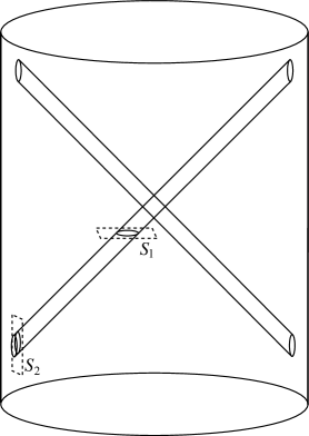
Figure 1: Surfaces $S_{1}$ and $S_{2}$ intersecting an incoming wavepacket.

For an outgoing particle there are corresponding surfaces after the scattering. The spacelike surface $S_{1}$ is taken to lie in the flat region near the origin as $N\to\infty$. The integral (8) then defines a flat-space creation operator for an incoming particle; with the envelope function $F_{\omega{\bf e}}$ omitted this would give a covariantly normalized plane wave. For the timelike region $S_{2}$ at the boundary we can use the dictionary [5, 6]

$$\lim_{r\to\infty}r^{4}\hat{\phi}(t,{\bf x})=\hat{\cal O}(t,{\bf\hat{x}})\ ,$$ (9)

where $\hat{\cal O}$ is the corresponding operator in the gauge theory on $S^{3}$. We define $\hat{\phi}$ to have canonical normalization as a five-dimensional field, so that the relation (9) defines an implicit normalization for $\hat{\cal O}$.

The integral on $S_{2}$ can therefore be expressed as an operator in the gauge theory. The analysis can immediately be extended to particles with masses of order the Kaluza–Klein scale $R^{-1}$ (which are therefore massless in ten dimensions). Classically these do not reach the boundary but do come very close, reaching $r\sim\omega$. They can still be created by $\hat{\phi}$ at the boundary but with an appropriate tunneling factor. In fact, the boundary behavior (6) acquires a term

$$r^{\nu-2}\ ,\quad\nu=(M^{2}R^{2}+4)^{1/2}\ ,$$ (10)

while the factor of $r^{4}$ in the operator relation (9) becomes $r^{2+\nu}$. The integral on $S_{2}$, and the corresponding integral for outgoing particles, are then

$$\alpha_{{\omega{\bf e}}-} = 2\nu\int dt\,d^{3}{\bf\hat{x}}\,G_{-}(t+\pi/2,|{\bf\hat{x}+e}|)e^{-i\omega t}\hat{\cal O}(t,{\bf\hat{x}})$$

$$\alpha_{{\omega{\bf e}}+} = 2\nu\int dt\,d^{3}{\bf\hat{x}}\,G_{+}(t-\pi/2,|{\bf\hat{x}-e}|)e^{-i\omega t}\hat{\cal O}(t,{\bf\hat{x}})\ .$$ (11)

These express the bulk creation and annihilation operators in terms of the operators in the boundary gauge theory. Incidentally, the solution $\phi_{\omega{\bf e}}$ is nonnormalizable, while the wave operator $\hat{\phi}$ couples to the normalizable modes that appear in the quantization of the field in AdS space. For any mass the product of these behaves as $r^{-4}$ at large $r$; combined with $r^{-1}$ from $\partial_{r}$, $r$ from $n^{r}$, and $r^{4}$ from the metric, the integrals defining $\alpha_{{\omega{\bf e}}\pm}$ are $r$-independent.

The flat-space S-matrix is then

$$S(I,O)=\lim_{N\to\infty}\Phi^{-1}\Biggl{\langle}\prod_{i\in I}\alpha_{{\omega_{i}{\bf e}_{i}}-}\ \prod_{j\in O}\alpha_{{\omega_{j}{\bf e}_{j}}+}\Biggr{\rangle}\ .$$ (12)

Here $I$ and $O$ denote the sets of incoming and outgoing particles, The proper energy of each particle is $\omega/R$ and the proper momentum is $\omega{\bf e}/R$. The expectation value is in the gauge theory on $S^{3}$, with the operators (11). The factor $\Phi$ accounts for the overlap of wavepackets,

$$\Phi=\int dt\,d^{4}{\bf x}\,\int_{S^{5}}d^{5}x^{\prime}\,\prod_{i\in I\cup O}F_{\omega_{i}{\bf e}_{i}}(t,{\bf x})\psi_{i}(x^{\prime})\ .$$ (13)

Here $\psi_{i}(x^{\prime})$ is the normalized wavefunction on $S^{5}$; for an $SO(6)$ singlet the net contribution of the compact space is $(V_{S^{5}})^{(2-n)/2}$. The proper momenta in the $S^{5}$ direction are of order $1/R$ and so vanish in the limit: the scattering process is restricted to a five-dimensional plane. To study processes with nonzero momenta in the $S^{5}$ directions would require the use of high representations of $SO(6)$, scaling with $N$.

Consider now corrections to free propagation, as depicted in figure 2.

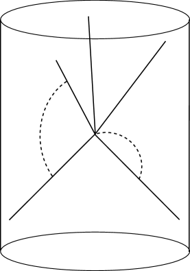
Figure 2: Interactions (dashed lines) correcting the free propagation of wavepackets.

Of course, these same processes are present in flat space, so they will change the S-matrix formula only to the extent that interactions at distances of order the horizon size are important. The characteristic size of the scattering region is set by the external momenta and so scales as $\omega^{-1}$. Thus, the interaction corrections will only be dangerous if they are IR divergent. In five dimensions even with massless particles amplitudes at generic momenta are IR convergent. This is a flat-spacetime result but in general one expects that IR diverenges are exacerbated by positive curvature and reduced by negative curvature [10]. This appears to be the case here as well, for example from examination of the gauge boson propagator in ref. [11].

Ref. [6] discusses various more subtle ways in which the relation (9) may fail due to interactions. However, we believe that our result for the S-matrix is robust. A local perturbation in the gauge theory is expected to correspond to a local disturbance on the boundary of AdS space; this is fully consistent with interactions in the Euclidean case [2], for example. This disturbance will propagate into the interior of AdS space as a particle or multiparticle state; appropriate kinematics then produces the S-matrix. We have used local fields (9) to derive the LSZ formula and of course the theory in the bulk is not a local field theory. However, we have used the field relation only in a very weak sense, essentially its vacuum to one-particle matrix element — there is no assumption that field theory, or locality, holds in the interaction region. In particular, we see no obstacle to assuming that the LSZ expression holds for arbitrarily large proper energies, of order the string scale, the Planck scale, or beyond. Note however that the proper energy is held fixed as $N\to\infty$.

It would be interesting to subject the S-matrix result (12) to various tests. However, many of its required properties, such as $SO(9,1)$ invariance, will not be manifest but instead must be taken as predictions for the behavior of the gauge theory. It may be possible to analyze the pole structure using the OPE in the gauge theory.

The final expression (12) in the gauge theory involves three energy–momentum scales: order 1 (in coordinate units) from the separation of the sources and the curvature of $S^{3}$, order $\omega\sim N^{1/4}$ from the incoming and outgoing waves, and order $\omega^{1/2}$ from the envelope function. One could also include a simpler object, in which the envelope functions are omitted and so one integrates the sources and detectors over times and angles (perhaps with spherical harmonics). This still gives the flat spacetime S-matrix but now with some average over external momenta because the kinematics of the scattering depends on its location, and also with the possible complication of multiple scattering from the periodicity of motion in AdS spacetime. Thus, flat-spacetime physics is obtained in the large-$N$ limit of a two-scale object, with momenta of order 1 and of order $g_{\rm s}N^{1/4}$. Further, the large momenta appear only in the time direction of the gauge theory. Incidentally, there seems to be no simple distance–energy relation such as there is in one-scale processes [1, 12].

Appendix

To analyze wavepackets with $\hat{e}=(1,0,0,0)$ it is convenient to use coordinates $(\rho,{\bf y})$ with $\bf y$ a three-vector, as defined by

$${\bf x}=(\tan\rho,{\bf y}/\cos\rho)\ .$$ (A.1)

The classical trajectory of interest is simply

$$\rho=t\ ,\quad{\bf y}=0\ .$$ (A.2)

In these coordinates the metric is

$$ds^{2}=\frac{R^{2}}{\cos^{2}\rho}\Biggl{[}-(1+y^{2})dt^{2}+d\rho^{2}+d{\bf y}\cdot d{\bf y}-\frac{({\bf y}\cdot d{\bf y})^{2}}{1+y^{2}}\Biggr{]}\ .$$ (A.3)

The d’Alembertian is

$$R^{2}\nabla^{2}=-\frac{\cos^{2}\rho}{1+y^{2}}\partial_{t}^{2}+\cos^{5}\rho\partial_{\rho}(\cos^{-3}\rho\partial_{\rho})+\cos^{2}\rho(\partial_{\bf y}\cdot\partial_{\bf y}+\partial_{\bf y}\cdot{\bf y}\,{\bf y}\cdot\partial_{\bf y})\ .$$ (A.4)

We seek a solution of the form

$$\phi=\exp\Bigl{[}i\omega f(t,\rho)-\omega y^{2}g_{1}(\rho)-\omega(t-\rho)^{2}g_{2}(\rho)+h(\rho)\Bigr{]}\ .$$ (A.5)

We are interested in the case $\omega\gg 1$ and so make an analysis of geometric optics (WKB) type. The first term in the exponent is the rapidly varying phase. The second and third terms produce the envelope in space and time; it follows that $\bf y$ and $t-\rho$ are of order $\omega^{-1/2}$.

Expanding $\nabla^{2}\phi=0$ in powers of $\omega$, the term of order $\omega^{2}$ is

$$\omega^{2}[(\partial_{t}f)^{2}-(\partial_{\rho}f)^{2}]=0$$ (A.6)

with solution $f=\rho-t$. At order $\omega$,

$$\omega\cos^{2}\rho\Bigl{[}-\omega y^{2}-2i\omega y^{2}g^{\prime}_{1}-2i\omega(t-\rho)^{2}g^{\prime}_{2}+2ih^{\prime}+3i\tan\rho-2g_{1}+4\omega y^{2}g_{1}^{2}\Bigr{]}=0\ ,$$ (A.7)

where the prime is a $\rho$ derivative. Thus,

$$g_{1}^{\prime} = \frac{i}{2}-2ig_{1}^{2}\ ,$$

$$g_{2}^{\prime} = 0\ ,$$

$$h^{\prime} = -\frac{3}{2}\tan\rho-ig_{1}\ .$$ (A.8)

These are readily integrated. A simple particular solution, which we will use henceforth, is

$$g_{1}=g_{2}=\frac{1}{2}\ ,\quad h=\frac{3}{2}\ln\cos\rho-\frac{i\rho}{2}\ .$$ (A.9)

At the origin this solution is of the form (6) with

$$F_{\omega{\bf e}}(t,{\bf x})=\exp\biggl{\{}-\frac{\omega}{2}\Bigl{[}x_{\perp}^{2}+(t-{\bf e}\cdot{\bf x})^{2}\Bigr{]}\biggr{\}}\ .$$ (A.10)

Here ${\bf x}_{\perp}$ is the part of $\bf x$ that is orthogonal to $\bf e$.

Very near the boundary, $r\sim\omega$, the WKB approximation breaks down. Here we can match onto the large-$r$ behavior

$$\phi=A(t,{\bf\hat{x}})\frac{e^{-i\omega t}}{r^{2}}H^{2,1}_{2}(\omega/r)\ ,$$ (A.11)

where the variation of $A(t,{\bf\hat{x}})$ is slow compared to the remaining factors. The superscripts $1,2$ on the Bessel function refers to the behavior at $t=\pm\pi/2$. In the regime $\omega\gg r\gg 1$ both the large-$r$ and WKB expressions are valid and so we can match, with the result

$$A(t,{\bf\hat{x}})=-ie^{\pm i\pi\omega/2}(\pi\omega/2)^{1/2}\exp\biggl{\{}-\frac{\omega}{2}\Bigl{[}|{\bf\hat{x}}\mp{\bf e}|^{2}+(t\mp\pi/2)^{2}\Bigr{]}\biggr{\}}\ .$$ (A.12)

The $r\gg\omega$ behavior of the Bessel function then gives the wavepacket on the boundary,

$$G_{\pm}(\tau,\theta)=-e^{\pm i\pi\omega/2}(2/\omega)^{3/2}\pi^{-1/2}\exp\biggl{\{}-\frac{\omega}{2}[\theta^{2}+\tau^{2}]\biggr{\}}\ .$$ (A.13)

For scalars with masses of order the Kaluza–Klein scale $R^{-1}$, the trajectory and WKB analysis are unaffected for $r$ less than $\omega$. The effect of the mass is then simply to change the order of the Bessel function to $\nu$, and the result for the wavepacket is

$$G_{\pm}(\tau,\theta)=e^{\pm i\pi(\omega+\nu)/2}(2/\omega)^{\nu-1/2}\Gamma(\nu)\pi^{-1/2}\exp\biggl{\{}-\frac{\omega}{2}[\tau^{2}+\theta^{2}]\biggr{\}}\ .$$ (A.14)

References

- [1] J. Maldacena, Adv. Theor. Math. Phys. 2, 231 (1998) hep-th/9711200.
-
[2]
S. S. Gubser, I. R. Klebanov, and A. M. Polyakov,
Phys. Lett. B428, 105 (1998) hep-th/9802109;
E. Witten, “Anti-de Sitter Space and Holography,” hep-th/9802150. - [3] K. Wilson, Rev. Mod. Phys. 55, 515 (1983).
-
[4]
E. Witten, talk at Strings ’98,
http://www.itp.ucsb.edu/online/strings98/witten/ ;
O. Aharony and T. Banks, “Note on the Quantum Mechanics of M Theory,” hep-th/9812237. - [5] V. Balasubramanian, P. Kraus, and A. Lawrence, “Bulk vs. Boundary Dynamics in Antide Sitter Spacetime,” hep-th/9805171.
- [6] T. Banks, M. R. Douglas, G. T. Horowitz, and E. Martinec, “AdS Dynamics from Conformal Field Theory,” hep-th/9808016.
-
[7]
V. Balasubramanian, P. Kraus, A. Lawrence, and S. P. Trivedi,
“Holographic Probes of Anti-de Sitter Spacetimes,”
hep-th/9808017;
V. Balasubramanian, S. Giddings, and A. Lawrence, work in progress. - [8] G. T. Horowitz and H. Ooguri, Phys. Rev. Lett. 80, 4116 (1998) hep-th/9802116.
- [9] I. Bena and J. Polchinski, work in progress.
- [10] C. G. Callan and F. Wilczek, Nucl. Phys. B340, 366 (1990).
- [11] E. D’Hoker and D. Z. Freedman, “Gauge Boson Exchange in ,” hep-th/9809179.
- [12] L. Susskind and E. Witten, “The Holographic Bound in Anti-de Sitter Space,” hep-th/9805114; A. W. Peet and J. Polchinski, “UV / IR Relations in AdS Dynamics,” hep-th/9809022.