January 1999

Worldsheet Fluctuations and the Heavy Quark
Potential in the AdS/CFT Approach

J. Greensite^ab and P. Olesen^c

	a Physics and Astronomy Dept. San Francisco State Univ.,
	San Francisco, CA 94117 USA. E-mail: greensit@stars.sfsu.edu
	b Theoretical Physics Group, Mail Stop 50A-5101,
	Lawrence Berkeley National Laboratory, Berkeley, CA 94720 USA.
	c The Niels Bohr Institute, Blegdamsvej 17,
	DK-2100 Copenhagen Ø, Denmark. E-mail: polesen@nbi.dk

Abstract

We consider contributions to the heavy quark potential, in the AdS/CFT approach to SU(N) gauge theory, which arise from first order fluctuations of the associated worldsheet in anti-deSitter space. The gaussian fluctuations occur around a classical worldsheet configuration resembling an infinite square well, with the bottom of the well lying at the AdS horizon. The eigenvalues of the corresponding Laplacian operators can be shown numerically to be very close to those in flat space. We find that two of the transverse world sheet fields become massive, which may have implications for the existence of a Lüscher term in the heavy quark potential. It is also suggested that these massive degrees of freedom may relate to extrinsic curvature in an effective $D=4$ string theory.

1 Introduction

Maldacena’s conjecture [1], relating the large $N$ expansion of conformal fields to string theory in a non-trivial geometry, has led to the hope that non-perturbative features of large $N$ theories may be understood. Witten’s extension [2] of this conjecture to non-supersymmetric gauge theories, such as large $N$ QCD in four dimensions, provides a new and elegant approach to the study of gauge theory at strong couplings.

In Witten’s approach the heavy quark potential has a linear behaviour [2, 3, 4, 5]. In this approach the temperature $T$ in the higher dimensional theory acts as an ultraviolet cutoff, and the strong coupling $g_{YM}^{2}N$ is the bare coupling at the scale $T$. The problem is, of course, how to extend this to lower coupling, and whether one encounters a phase transition on the way, as discussed in [6].

In the approach of refs. [2, 3, 4, 5] the interquark potential has been extracted at the saddle point. In the present paper we extend this by including fluctuations of the world sheet to first order. The present paper was initiated as a sequel to a previous letter [7], where we have called attention to two features of strong-coupling, planar $QCD_{3}$ in the saddle point approximation, which do not entirely agree with expectations based on lattice QCD. First, there is the fact that the glueball mass is essentially independent of string tension in the strong-coupling supergravity calculation [8], and goes to a finite constant in the $\sigma\rightarrow\infty$ limit. This is quite different from the behavior in strong-coupling lattice gauge theory, where a glueball is understood as a closed loop of electric flux whose mass tends to infinity in the infinite tension limit, and it suggests that truly different physical mechanisms may underlie the mass gap in the two cases. The second point concerns the existence of a universal Lüscher term of the form $-c/L$ in the interquark potential. Here $c$ is a numerical, coupling independent, constant. Recent lattice Monte Carlo simulations [9] indicate the presence of such a term in $QCD_{3}$, with a value of $c$ consistent with that of a bosonic string, although there is a caveat that $-c/L$ represents a quite small correction to the dominating linear potential, and the magnitude of $c$ is not yet well determined numerically. Following the approach of refs. [2, 3, 4, 5], we have found that the interquark potential extracted from the saddle point action of a classical worldsheet in $AdS_{5}\times S_{5}$, has no Lüscher term at all, which seems to contradict the existing trend in the Monte Carlo data.

It is quite possible, however, that the Lüscher term arises beyond the classical worldsheet approximation, when quantum fluctuations of the worldsheet in $AdS_{5}\times S_{5}$ are taken into account [10, 11, 12]. This question is the main motivation for the work reported in the present paper.

In Section 2 we study the background field in the saddle point for large interquark distances. It turns out that the radial AdS coordinate $U$ [1] of the string worldsheet is situated at the horizon, except for a small interval in parameter space near the end points $\sigma=\pm L/2$, where $U$ is forced to shoot up to infinity. In Section 3 we introduce Kruskal-like coordinates, and discuss the near-flatness of this metric at the horizon, in the $g^{2}_{YM}N\rightarrow\infty$ limit. The eigenvalues and eigenfunctions for the relevant Laplacians are then shown to be essentially the same as in the completely flat case, with the contour of the classical worldsheet bringing the problem into the form of an infinite square well.

In Section 4 we discuss the expansion of the action to the first non-trivial order. It is found that two of the transverse worldsheet coordinates become massive, and do not contribute to the Lüscher term. We argue that, due to the vanishing curvature in the $g^{2}_{YM}N\rightarrow\infty$ limit, the fermion and ghost contributions will have essentially flat-space contributions to $-c/L$, although we do not claim to show this explicitly.

If the fermionic and ghost contributions are in fact similar to flat space, then a possible consequence is that the Lüscher term has a sign opposite to the one extracted from the Monte Carlo data. The Lüscher term is essentially the Casimir energy of a string with fixed ends. For a superstring in flat space with Ramond boundary conditions, there is an exact cancellation of bosonic and fermionic contributions to the Casimir energy, and the Lüscher term vanishes. In the case of Neveu-Schwartz boundary conditions, bosonic and fermionic zero-point energies contribute with the same sign, and this is what leads to a tachyonic state for a free string. However, when the GSO projection is taken into account and the tachyonic state is removed, we again have a massless ground state and a vanishing Lüscher term. The relation between having a tachyonic ground state for the free string, and an attractive potential from the Lüscher term, is discussed in ref. [13].

Since the string worldsheet, in the AdS/CFT approach, is intended to describe the dynamics of the QCD string between massive quarks, then presumably the appropriate boundary conditions are Neveu-Schwartz, with a GSO projection removing the lowest state. Taking account of the mass term for two of the transverse degrees of freedom, and assuming (as curvature becomes negigible in the $g^{2}_{YM}N\rightarrow\infty$ limit) that the rest of the degrees of freedom contribute to the Casimir energy as they do in flat space, the result is a “wrong-sign” Lüscher term. We must emphasize, however, that this is a very tentative conclusion, and one which does not take the Ramond-Ramond background into consideration.

So far these results refer to QCD in three dimensions. Section 5 contains a brief discussion of the four dimensional case. Finally, in section 6, we suggest that in four dimensions the massive world sheet fields may relate to extrinsic curvature terms in an effective 4D string theory. In Section 7 we conclude. It is noted that if our tentative result for the sign of the Lüscher term is correct, it implies that the strong coupling supergravity approach to QCD does not correspond to QCD defined on a lattice.

2 The saddle point field for large interquark distances

As explained in ref. [2, 4], spatial Wilson loops in D=3 planar Yang-Mills theory are computed, in the supergravity approach, from the dynamics of worldsheets in the near-extremal background metric

$$ds^{2}=\alpha^{\prime}\left\{\frac{U^{2}}{R^{2}}\left((1-U_{T}^{4}/U^{4})dt^{2}+\sum_{i}dx_{i}^{2}\right)+\frac{R^{2}}{U^{2}}\frac{dU^{2}}{1-U_{T}^{4}/U^{4}}+R^{2}d\Omega_{5}^{2}\right\}.$$ (2.1)

The boundary of the worldsheet is a rectangle in the $x_{1}-x_{2}$ plane at $U=\infty$, whose interior, specified by $x_{1}=\sigma,~{}x_{2}=\tau$ with $|\sigma|\leq{L\over 2}$, and $|\tau|\leq{Y\over 2}$, parametrizes the worldsheet of a $L\times Y$ Wilson loop with $Y\gg L$. The classical worldsheet, in the $Y\rightarrow\infty$ limit, is given by $x_{1}(\sigma,\tau)=\sigma,~{}x_{2}(\sigma,\tau)=\tau$, and $U(\sigma)$ determined implicitly from

$$\frac{L}{2}-\sigma=\frac{R^{2}}{U_{0}}\int_{U/U_{0}}^{\infty}\frac{dy}{\sqrt{(y^{4}-1)(y^{4}-1+\epsilon)}}$$ (2.2)

with

$$U_{0}=U(\sigma=0),~{}~{}~{}~{}\epsilon=1-U_{T}^{4}/U_{0}^{4},~{}~{}~{}~{}R^{2}=\sqrt{4\pi g^{2}_{YM}N},~{}~{}~{}~{}U_{T}=R^{2}b$$ (2.3)

The metric (2.1) is relevant for the calculation of the boson and fermion contributions to the action. In general, since the background field $U=U(\sigma)$ is a non-trivial function of $\sigma$, one cannot expect that world sheet supersymmetry is preserved in the presence of this background field. On the other hand, a graph of $U(\sigma)$ in the range $\sigma\in[-{L\over 2},{L\over 2}]$ looks very much like an infinite square well at large $L$, as seen in Fig. 1. Starting at $U(-{L\over 2})=\infty$, $U(\sigma)$ drops precipitously to $U(\sigma)\approx U_{0}\approx U_{T}$, remaining almost constant in a range $[{L\over 2}+d,{L\over 2}-d]$ where $d\ll L$, and then shoots back up to $U=\infty$ at $\sigma={L\over 2}$. The fact that the classical worldsheet coordinate $U(\sigma)$ is nearly constant for most of the range of $\sigma$ is, of course, very relevant for a saddlepoint calculation, where we include the effect of gaussian fluctuations around the classical worldsheet.

Figure 1: String contours $U(x)$ for various $\epsilon=1-(U_{T}^{4}/U_{0}^{4})$, in units of $U_{T}=R^{2}b$. The asymptotes of each curve lie at $x=\pm L/2$. Note the approach to the horizon (here at $U=1$), as $\epsilon\rightarrow 0$.

We will need expressions for $U(\sigma)$ both near and away from $\sigma=\pm{L\over 2}$. Denoting $y(\sigma)=U(\sigma)/U_{0}$, we have

$$dy/d\sigma=b\sqrt{(y^{4}-1)(y^{4}-1+\epsilon)}$$ (2.4)

where $\epsilon=1-U_{T}^{4}/U_{0}^{4}$ was found [7] to be related to the interquark distance $L$ by

$$\epsilon\approx e^{-2bL}.$$ (2.5)

Away from the endpoints at $\sigma=\pm{L\over 2}$ make the trial expansion

$$y(\sigma)\approx 1+\delta(\sigma),~{}{\rm with}~{}|\delta(\sigma)|\ll 1.$$ (2.6)

and then linearize eq.(2.4),

$$d\delta/d\sigma\approx 2b\sqrt{\delta(4\delta+\epsilon)},$$ (2.7)

which is valid as long as $\delta$ stays small. Integrating we obtain

$$\ln(2\sqrt{\delta}+\sqrt{4\delta+\epsilon})=2b\sigma+\ln\sqrt{\epsilon},$$ (2.8)

where we used the boundary condition that $y=1$, and hence $\delta=0$, for $\sigma=0$. Solving this equation for $\delta$, we get

$$y(\sigma)\approx 1-\exp(-2bL)/8+[\exp(-4b(L/2+\sigma))+\exp(-4b(L/2-\sigma))]/16.$$ (2.9)

Thus, for $|\sigma|<L/2$ the corrections to $y=1$ are exponentially small, and $U(\sigma)\approx U_{0}$ is essentially constant.

For $|\sigma|\rightarrow{L\over 2}$ this analysis breaks down, since $\delta$ is not small. From the relation

$$\frac{L}{2}-\sigma=\frac{R^{2}}{U_{0}}\int_{U/U_{0}}^{\infty}\frac{dy}{\sqrt{(y^{4}-1)(y^{4}-1+\epsilon)}}\approx\frac{R^{2}U_{0}^{2}}{3U^{3}}\approx\frac{1}{3by^{3}},$$ (2.10)

using $U_{0}\approx U_{T}=R^{2}b$, we see that

$$U\approx\frac{R^{2}b}{(3b(L/2-\sigma))^{1/3}},~{}{\rm for}~{}\sigma\rightarrow L/2$$ (2.11)

in the neighbourhood of $|\sigma|\rightarrow{L\over 2}$. A plot of the exact solution for $y(\sigma)$ at $bL=30$, and the two asymptotic solutions (2.9) and (2.11), is shown in Fig. 2.

Figure 2: A $\sigma/(L/2)$ versus $U/U_{0}$ plot of the exact solution for $bL=30$, compared to the two asymptotic solutions. The solution valid for $\sigma\approx L/2$ approaches the exact solution near $y=1.25$, whereas the $|\sigma|<L/2$ solution starts to deviate from the exact solution near $\sigma\approx 0.925(L/2)$.

According to eq. (2.9) and Fig. 1, the classical solution for $U(\sigma)$ is almost constant in some interval $[-{L\over 2}+d,{L\over 2}-d]$. To estimate $d$, we can first ask for the value close to $\sigma={L\over 2}$ where the asymptotic solutions (2.9) and (2.11) are equal. This happens for

$$\frac{\sigma}{L/2}\approx 1-\frac{.63}{bL}.$$ (2.12)

A more stringent criterion, arrived at numerically, is to ask where $y(\sigma)$ deviates from $y=1$, at large $L$, by more than $10^{-3}$. With this criterion for $d$, we find that $d<1.5/b$, approximately, obtained from the solutions for $y(\sigma)$ at various $L$ shown in Fig. 3.

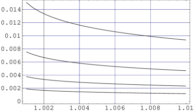
Figure 3: A plot of $1-\sigma/(L/2)$ as a function of $y=U/U_{0}$. The curves from the top to the bottom correspond to $bL$=200, 400, 800, and 1600, respectively. If we fix the upper limit on $d$ by requiring that $y$ should only deviate from 1 by $10^{-3}$, corresponding to the left side of the figure, we see that $1-\sigma/(L/2)$ decreases like $1/L$ to a high accuracy, because in going from the top to the bottom at $y=1.001$, the distance between the successive curves decreases by a factor two.

3 Eigenvalues of Laplacians in the AdS background

We would like to make an expansion around the saddle point. In order to do this, it is convenient to use different variables than $U$ and $t$, because of the singular form of the metric (2.1). We therefore introduce the Kruskal-like coordinates for $U>U_{T}$

$$T=\frac{\sqrt{2}~{}R^{2}}{U_{T}}~{}e^{-\pi/4}e^{\tan^{-1}(U/U_{T})}\sqrt{\frac{U-U_{T}}{U+U_{T}}}\cos\left(\frac{2U_{T}t}{R^{2}}\right),$$

$$Z=\frac{\sqrt{2}~{}R^{2}}{U_{T}}~{}e^{-\pi/4}e^{\tan^{-1}(U/U_{T})}\sqrt{\frac{U-U_{T}}{U+U_{T}}}\sin\left(\frac{2U_{T}t}{R^{2}}\right).$$ (3.1)

These expressions are valid in Euclidean space, and in Minkowski space the sine and cosine are replaced by the hyperbolic sine and cosine, respectively. The time variable $t$ is periodically identified by $t\rightarrow t+\pi/b$, with $U_{T}=bR^{2}$. In these coordinates

$$ds^{2} = \alpha^{\prime}\left\{\frac{(U^{2}+U_{T}^{2})(U+U_{T})^{2}e^{\pi/2}}{8R^{2}U^{2}}e^{-2\tan^{-1}(U/U_{T})}\left(dT^{2}+dZ^{2}\right)\right.$$ (3.2)

$$+ \left.\frac{U^{2}}{R^{2}}\sum_{i}dx_{i}^{2}+R^{2}d\Omega_{5}^{2}\right\},$$

so that the metric is now symmetric in terms of the new variables $Z$ and $T$. As usual with the (Euclidean) Kruskal metric, $U$ should be considered as a function of $T^{2}+Z^{2}$ through the equation ($U>U_{T}$)

$$Z^{2}+T^{2}=\frac{2R^{4}e^{-\pi/2}}{U_{T}^{2}}e^{2\tan^{-1}(U/U_{T})}\frac{U-U_{T}}{U+U_{T}}.$$ (3.3)

It should be noticed that the metric (3.2) is flat up to exponentially small terms, except at the end points $\sigma=\pm L/2$.

The saddlepoint contribution to the spatial Wilson loop is given by simply evaluating the Nambu action of the classical worldsheet in this metric [2, 4], and is found to be

$$S_{cl}={U_{T}^{2}\over 2\pi R^{2}}YL$$ (3.4)

We are interested now in the contribution from gaussian fluctuations around the saddlepoint, which involve the bosonic, fermionic, and ghost degrees of freedom, in the limit of very large $R$.

In the $R\rightarrow\infty$ limit the curvature of the 5-sphere (as well as the curvature of AdS space) vanishes, and the contribution of each degree of freedom associated with the 5-sphere is identical to the corresponding flat-space value, i.e. $-\pi Y/24L$. Likewise, fluctuations around the classical worldsheet in AdS space in the neighborhood of the horizon, i.e. $\sigma\in[-{L\over 2}+d,{L\over 2}-d]$, are essentially fluctuations in flat space, and the relevant differential operators are either the flat-space 2D Laplacian, or, as we shall see in the next section, this operator plus a mass term. Thus, for example, the eigenstates $\psi(\sigma,\tau)$ of

$$\partial^{2}_{M}\equiv\partial_{a}G_{MM}[U_{cl}(\sigma)]\partial^{a}$$ (3.5)

will be identical to eigenstates of the flat-space 2D Laplacian, i.e.

$$\psi(\sigma,\tau)\propto\sin[\alpha(\sigma+c)]e^{i\omega\tau}$$ (3.6)

away from the $\sigma=\pm{L\over 2}$ endpoints. The eigenvalue spectrum is determined by the boundary conditions $\psi(\sigma,\tau)=0$ at $\sigma=\pm{L\over 2}$ (meaning that fluctuations vanish at the Wilson loop perimeter). In flat space these conditions yield the usual result that

$$\alpha^{flat}_{n}={n\pi\over L}~{}~{},~{}~{}~{}~{}~{}~{}c=L/2$$ (3.7)

In AdS space the values for $\alpha$ are slightly different, owing to the fact that eq. (3.6) breaks down for ${L\over 2}-|\sigma|<d$. Very close to the endpoints, the operator $\partial^{2}_{M}$ becomes $\partial_{a}U^{2}(\sigma)\partial_{a}$. We solve for the eigenfunctions in this region by making separation ansatz $\psi(\tau,\sigma)=\Theta(\tau)S(\sigma)$, and find for the eigenvalue equation $\partial_{i}(U^{2}\partial_{i})\psi=\Lambda\psi$ near the end points

$$\partial_{\sigma}^{2}S+\frac{2}{3(L/2-\sigma)}\partial_{\sigma}S-\tilde{\Lambda}(L/2-\sigma)^{2/3}S-\lambda S=0,~{}{\rm where}~{}\tilde{\Lambda}=\frac{(3b)^{2/3}}{R^{4}b^{2}}\Lambda.$$

$$\partial^{2}_{\tau}\Theta=-\lambda\Theta.$$ (3.8)

Here $\lambda$ is a separation constant. The equation for $\Theta$ is the same as for the $\partial^{2}$ operator, whereas for the function $S$ in the neighborhood of the endpoints there are two solutions, namely one for which $S$ vanishes, in $\sigma\rightarrow{L\over 2}$ limit, as

$$S\approx{\rm const.}~{}(L/2-\sigma)^{5/3}$$ (3.9)

and one where $S$ goes to a non-zero constant for $\sigma\rightarrow{L\over 2}$. The solution vanishing at the endpoints is the one which is relevant for worldsheet fluctuations. Away from the endpoints, $\psi(\sigma,\tau)$ has the harmonic form shown in eq. (3.6). The “end point solution” (3.9) vanishes more rapidly than the sine function near $\sigma=\pm{L\over 2}$, which is due to the fact that in eq. (3.8) the first derivative $S^{\prime}$ is multiplied by a large factor, and hence is forced to be small.

We can now make a rough estimate of how the eigenvalues of $\partial^{2}_{M}$ compare to those of the flat-space operator, based on the fact that $\psi(\sigma,\tau)$ falls much more rapidly to zero, near the endpoints at $\sigma=\pm{L\over 2}$, than the sine function. This allows us to approximate $\psi(\sigma,\tau)$ as a harmonic function in the range $[-{L\over 2}+d,{L\over 2}-d]$, and equal to zero outside this range. Then

$${|\alpha_{n}-\alpha^{flat}_{n}|\over\alpha^{flat}_{n}} \sim {{n\pi\over L-d}-{n\pi\over L}\over{n\pi\over L}}$$ (3.10)

$$\sim O\Bigl{[}{d\over L}\Bigr{]}$$

$$\sim O\Bigl{[}{1\over bL}\Bigr{]}$$

Since the flat-space eigenvalues for the massless Laplacian lead to a Lüscher term of $O(1/L)$, these small deviations can only lead to a further correction, in the AdS case, of still higher order in $1/L$. For the massive Laplacian the situation is, however, different, as we shall see in the next section.

A similar observation presumably applies to the fermionic and ghost degrees of freedom The associated differential operators in $\sigma,~{}\tau$ again only deviate from the corresponding flat-space case in a region near the endpoints, where the derivatives are multiplied by a factor of $U(\sigma)$; this region is a very small fraction (of order $1/L$) of the full interval. Eigenmodes of these operators will have to be nearly constant in the “shootup” region near the endpoints, where $U(\sigma)\rightarrow\infty$. However, as in the case of the bosonic modes, this slight modification of the eigenmodes will only affect the values of the determinants at higher orders in $1/L$.

4 The bosonic action and the necessity of massive fields

We want now to study the bosonic action, keeping only quadratic terms in the 8 transverse variables ($Z,T,x_{3},...$). We start from the partition function

$${\cal Z}=\int{\cal D}X\sqrt{G}\exp\left(\frac{1}{2\pi\alpha^{\prime}}\int d^{2}\sigma\sqrt{\det G_{MN}(X(\sigma))\partial_{a}X^{M}\partial_{b}X^{N}}\right),$$ (4.1)

where we integrate over the 10 variables $X^{M}$, and insert a factor $\sqrt{G}$ in order to have a measure which is invariant with respect to changes of the coordinates entering the $AdS_{5}\times S_{5}$. We also want to choose a gauge where $\sigma,\tau$ are identified with $x_{1},x_{2}$. The measure factor in (4.1) can then be exponentiated in the form

$$\sqrt{G}=\exp\left(\Lambda^{2}\int d^{2}\sigma\sqrt{h}\ln G\right).$$ (4.2)

Here $h$ is the measure associated with the world sheet variables, so $\sqrt{h}=\alpha^{\prime}U^{2}/R^{2}$, and $\Lambda$ is a ultraviolet cutoff. This form of the exponentiation is reparametrization invariant. Because of the absence of a $1/2\pi\alpha^{\prime}$ factor in the exponentiated version of $\sqrt{G}$, this factor will only contribute to terms of order $\alpha^{\prime}$ in the effective action. We shall not consider this order, and we therefore ignore the $\sqrt{G}$ contribution in the following.

Now, if we expand the action, keeping only second order terms, we get

$$S\approx(1/2\pi)\int d^{2}\sigma\left\{U^{2}/R^{2}+(1/2)\left[(U^{2}_{T}/R^{2})\left((\partial_{i}Z)^{2}+(\partial_{i}T)^{2}+(\partial_{i}x_{3})^{2}\right)+R^{2}(\partial_{i}y^{M})^{2}\right]\right\},$$ (4.3)

where the $y$’s refer to the 5-sphere, and where we took $x_{1},x_{2}$ to be longitudinal. Of course, it is important to keep all second order terms. To this end, we need to notice that the $U^{2}$ in the first term is given as a function of $Z,T$. Exactly at the horizon $Z=T=0$, and $Z^{2}+T^{2}$ therefore represent the small, second order deviations of the radial variable from its value at the horizon,

$$U\approx U_{T}+(U_{T}^{3}/R^{4})(Z^{2}+T^{2}).$$ (4.4)

Inserting in eq. (4.3), we find to 2nd order in the fluctuations

$$S \approx (1/2\pi)\int d^{2}\sigma(U_{T}^{2}/R^{2}+(U_{T}^{2}/2R^{2})[(\partial_{i}Z)^{2}+(\partial_{i}T)^{2}+(4U_{T}^{2}/R^{4})(Z^{2}+T^{2})]$$ (4.5)

$$+(U_{T}^{2}/2R^{2})(\partial_{i}x_{3})^{2})+(R^{2}/2)(\partial_{i}y^{M})^{2}),$$

which shows that the fields $Z,T$ have mass terms with coefficients $4U_{T}^{2}/R^{4}=4b^{2}$. Thus two bosonic degrees of freedom, originally associated with the $U,~{}t$ coordinates, have become massive, and it is not hard to see why such a “potential” term must exist: The boundary of the worldsheet lies at $U=\infty$, yet the preferred position of the string, as $L\rightarrow\infty$, lies at the black hole horizon $Z=T=0$. The first term in the integral gives the leading contribution $(U_{T}^{2}/2\pi R^{2})YL$, corresponding to a 3D string tension

$${\cal T}_{3}={U_{T}^{2}\over 2\pi R^{2}}={R^{2}b^{2}\over 2\pi}$$ (4.6)

derived in refs. [2, 4, 5].

The Gaussian integral over $Z,T$ can be performed, e.g. by use of analytic regularization [14] ($\ln x=\partial x^{\beta}/\partial\beta$ for $\beta\rightarrow 0$). Since $Y\rightarrow\infty$, the sum over the “time-eigenvalues” can be replaced by an integral, which can be performed to give

$${\rm tr~{}ln}(-\nabla^{2}+4b^{2})=-(Y/\sqrt{4\pi})(\partial/\partial\beta)(\Gamma(\beta-1/2)/\Gamma(\beta))\sum_{n=1}^{\infty}((n\pi/L)^{2}+(4b^{2}))^{-\beta+1/2}$$ (4.7)

with $\beta\rightarrow 0$. The sum over $n$ can be carried out and the limit $\beta\rightarrow 0$ can be performed to give [14]

$${\rm tr~{}ln}(-\nabla^{2}+4b^{2})=-\frac{YL}{\pi}b^{2}(-1+\ln(4b^{2}/\mu^{2}))-Yb\left[1+\frac{2}{\pi}\sum_{n=1}^{\infty}\frac{1}{n}K_{1}(4nbL)\right].$$ (4.8)

Here $\mu$ is an ultraviolet cutoff, which occurs in the heat kernel method, which gives cutoff dependent terms proportional to $\mu^{2}$ and $b^{2}\ln\mu^{2}$. The $\mu^{2}$ terms are present for all fields, and if we add the fermions they cancel completely. The logarithmic terms only occur for the massive fields (see e.g. [14]), and they combine with the $b^{2}\ln(4b^{2})$ term to give the result exhibited in (4.8).

Using the asymptotic expansion of the Bessel function valid for large $L$, we get

$${\rm tr~{}ln}(-\nabla^{2}+4b^{2})\approx-\frac{YL}{\pi}b^{2}(-1+\ln(4b^{2}/\mu^{2}))-Yb\left[1+\frac{1}{\sqrt{2\pi bL}}e^{-4bL}+...\right].$$ (4.9)

This can be compared to the massless case,

$${\rm tr~{}ln}(-\nabla^{2})=-\pi Y/12L.$$ (4.10)

It can be shown that this result follows by rewriting the sum over Bessel functions in eq. (4.9), by use of the following relation

$$\sum_{n=1}^{\infty}K_{1}(nz)/n=\pi^{2}/6z+(1/4){\bf C}z+(1/8)z\ln(z/(4\pi)^{2})-z/16+\pi/4$$ (4.11)

$$+ \pi\sum_{l=1}^{\infty}\left(\sqrt{1+4l^{2}\pi^{2}/z^{2}}-2l\pi/z-z/4l\pi\right),$$

where $\bf C$ is Euler’s constant, and taking the limit $b\rightarrow 0$. The first term on the right hand side gives the desired result for $b\rightarrow 0$ if we take $z=4bL$. For $bL$ large, the above expression is not useful, and the asymptotic expansion of the Bessel functions should then be used.

We have stressed, in the previous section, that curvature in $AdS_{5}\times S_{5}$ tends to zero in the $R\rightarrow\infty$ limit, and string fluctuations in the neighborhood of the horizon are essentially fluctuations in a flat-space metric. That being the case, how can we find a mass term in eq. (4.9) of $O(b^{2})$, which is finite in the $R\rightarrow\infty$ limit? At first sight, this seems a violation of the principle of equivalence. To understand what is going on, we first note that the metric coefficients in eq. (3.2) are all of order $R^{2}$ near the horizon. The integration in (4.5) runs from $-L/2$ to $+L/2$, but in fact the proper time along the horizon is of order $RL$. If we make a trivial change of variables, simply rescaling all coordinates (and parameters $\sigma,\tau$) by a factor of $R$ so metric coefficients are all $O(1)$ near the horizon, then the contribution to the action from the region along the horizon is approximately

$$S \approx (b^{2}/2\pi)\int^{+RY/2}_{-RY/2}d\tau\int^{+RL/2}_{-RL/2}d\sigma\Bigl{(}1+\frac{1}{2}[(\partial_{i}Z)^{2}+(\partial_{i}T)^{2}+(4b^{2}/R^{2})(Z^{2}+T^{2})]$$ (4.12)

$$+\frac{1}{2}(\partial_{i}x_{3})^{2})+(1/2b^{2})(\partial_{i}y^{M})^{2}\Bigr{)},$$

Here the mass term evidently tends to zero as $R\rightarrow\infty$, as one would expect from the equivalence principle. But this decrease is precisely compensated by the growth of the worldsheet along the horizon (as seen in the limits of integration) as $R$ increases. The end result of a gaussian integration is, of course, identical to eq. (4.9); one finds a finite, $R$-independent mass term in the trace log.

For the bosonic part we thus have two massive and six massless degrees of freedom. The contribution from the bosonic part of the string to the potential is thus

$${\rm Potential~{}from~{}bosons}=\frac{R^{2}b^{2}}{2\pi}\left(1-\frac{2}{R^{2}}\ln\frac{4b^{2}}{e\mu^{2}}\right)L-\frac{\pi}{4L}.$$ (4.13)

We see that bosonic contributions are responsible for a logarithmic correction to the lowest order result for the string tension (4.6), i.e.

$${\cal T}_{3}=\frac{R^{2}b^{2}}{2\pi}\left(1-\frac{2}{R^{2}}\ln\frac{4b^{2}}{e\mu^{2}}\right).$$ (4.14)

As $g^{2}_{YM}N\rightarrow\infty$, the curvature of AdS space tends to zero. If the contributions from the fermions and ghosts can really be obtained in the flat space limit near the horizon, as argued in the last section, then the resulting Lüscher term would be the same as if the calculation were done in flat space, with the contribution $-\pi/12L$ from two transverse bosonic modes removed. With either Ramond boundary conditions, or Neveu-Schwartz boundary conditions with the tachyon projected out, the result is a Lüscher term $+\pi/12L$. This term has the opposite sign relative to what is seen in lattice calculations. However, the fermions in the full AdS background really need to be investigated further, before this can be considered as a safe conclusion.

5 The potential in four dimensions

Let us consider the relevant metric [4] near the horizon $U\approx U_{T}$,

$$\frac{ds^{2}}{\alpha^{\prime}}\approx\frac{R^{3/2}}{3U_{T}^{1/2}}\frac{dU^{2}}{U-U_{T}}+\frac{3U_{T}^{1/2}}{R^{3/2}}(U-U_{T})dt^{2}\equiv dr^{2}+r^{2}d\theta^{2}\equiv dX^{2}+dY^{2},$$ (5.1)

with $X=r\cos\theta,~{}Y=r\sin\theta$ ($X,Y$ thus correspond to the coordinates previously denoted by $T,Z$ in the three dimensional case). Here we left out the four-sphere as well as the four $x$-coordinates, since these are not important for the following. Instead of finding the full Kruskal coordinates, we only look at the local ones near the horizon,

$$dr=\frac{R^{3/4}}{\sqrt{3}U_{T}^{1/4}}\frac{dU}{\sqrt{U-U_{T}}},$$ (5.2)

so

$$U-U_{T}=\frac{3U_{T}^{1/2}}{4R^{3/2}}r^{2}=\frac{3U_{T}^{1/2}}{4R^{3/2}}(X^{2}+Y^{2}).$$ (5.3)

Thus

$$\frac{ds^{2}}{\alpha^{\prime}}\approx\frac{9U_{T}}{4R^{3}}r^{2}dt^{2}+dr^{2}.$$ (5.4)

We have

$$R^{3/2}=g_{5}\sqrt{N/4\pi}=g_{YM}\sqrt{N/4\pi T}.$$ (5.5)

Because of periodicity of the angle, i.e. identification of $\theta\rightarrow\theta+2\pi$, corresponding to $t\rightarrow t+1/T$ (i.e. $T=b/\pi$), one therefore needs

$$\theta^{2}=\frac{9U_{T}}{4R^{3}}t^{2},~{}{\rm i.e.}~{}T=\frac{3U_{T}^{1/2}}{2g_{5}\sqrt{\pi N}}.$$ (5.6)

Using (5.3) we then have

$$U=U_{T}+\frac{3U_{T}^{1/2}}{4R^{3/2}}(X^{2}+Y^{2}).$$ (5.7)

We can now proceed as in the 3-d case. The expanded action is

$$S\approx\frac{1}{2\pi}\int d^{2}\sigma\left(\frac{U^{3/2}}{R^{3/2}}+\frac{1}{2}\left[(\partial_{i}X)^{2}+(\partial_{i}Y)^{2}\right]\right).$$ (5.8)

Using

$$\frac{U^{3/2}}{R^{3/2}}\approx\frac{U_{T}^{3/2}}{R^{3/2}}+\frac{9U_{T}}{8R^{3}}(X^{2}+Y^{2}),$$ (5.9)

this leads to an $X,Y$ (former $Z,T$) -dependent integrand

$$\frac{1}{2}\left[(\partial_{i}X)^{2}+(\partial_{i}Y)^{2}+\frac{9U_{T}}{4R^{3}}(X^{2}+Y^{2})\right].$$ (5.10)

with mass parameter

$$\frac{9U_{T}}{4R^{3}}=4\pi^{2}T^{2}.$$ (5.11)

We can now compute the contribution to the potential using the results in ref [14], and adding the leading terms (ignoring terms which are exponentially small), we get the string tension in four dimensions by use of analytic regularization ($\ln x=\partial x^{\beta}/\partial\beta$ for $\beta\rightarrow 0$)

$${\cal T}_{4} = \frac{8\pi}{27}g_{YM}^{2}NT^{2}\left[1+\frac{27}{2g_{YM}^{2}N}\left(1-\ln\frac{4\pi^{2}T^{2}}{\mu^{2}}\right)\right]$$ (5.12)

$$= \frac{8\pi}{27}g_{YM}^{2}NT^{2}\left[1-\frac{27}{2g_{YM}^{2}N}\ln\frac{4\pi^{2}T^{2}}{e\mu^{2}}\right].$$

Here $\mu$ is the arbitrary scale introduced in the last section.

We end this section by remarking again that the effective flatness of AdS space, in the strong-coupling limit, suggests that the fermi and ghost degrees of freedom contribute to the Lüscher term as in flat space. If this is so, then the naive counting argument of the last section again leads to the net result for the Lüscher term

$$+{\pi\over 12L}.$$ (5.13)

in the quark-antiquark potential. This should be compared to what has been used in fits to the lattice Monte Carlo data, namely

$$-{(d-2)\pi\over 24L}=-{\pi\over 12L}.$$ (5.14)

Thus the magnitude is the same, but the signs are opposite.

This result is based on the assumption that the worldsheet fermions essentially live in a flat space, so that the flat string action is relevant. Although we have given some plausibility arguments, this remains to be proven. However, if the result is true, it has been pointed out to us by Lüscher [15] that this has the far reaching consequence that supergravity in the limit $g^{2}_{YM}N\rightarrow\infty$ has nothing to do with QCD defined on the lattice, for any $N$ and with or without matter fields. The reason is that it has been shown rigorously by Bachas [16] that the heavy quark potential $V(L)$ is monotonic and concave. Thus,

$$V^{\prime}(L)\geq 0~{}{\rm and}~{}V^{\prime\prime}(L)\leq 0$$ (5.15)

for all $L$, contradicting a positive value of the Lüscher term.

6 Massive fields and extrinsic curvature

One of the most interesting questions in non-perturbative gauge theory, which the AdS/CFT correspondence may eventually address, concerns the form of the effective D=4 string theory describing the QCD string. In this connection, we would like to make a remark that may be relevant for the understanding of the existence of massive fields versus reparametrization invariance.

When the 1-loop contributions of two massive and two massless worldsheet modes are combined, one finds a result which is strongly reminiscent of string models with extrinsic curvature [18]. The extrinsic curvature $K^{i}_{ab}$ (=the second fundamental form) is given by

$$D_{a}D_{b}{\bf X}=K^{i}_{ab}{\bf N}_{i},~{}{\rm with}~{}{\bf N}_{i}{\bf N}_{k}=\delta_{ik}~{}{\rm and}~{}{\bf N}_{i}\partial_{a}{\bf X}=0,$$ (6.1)

where ${\bf X}(\sigma,\tau)$ is is the position vector for some surface, ${\bf N}_{i}$ are the normals, and $D_{a}$ is the covariant derivative with respect to the induced metric $g_{ab}=\partial_{a}X\partial_{b}X$. There are many expressions for the extrinsic curvature. Here we need in particular

$$K^{ia}_{b}K^{ib}_{a}=\left(\partial_{a}(\sqrt{g}g^{ab}\partial_{b}X)\right)^{2}.$$ (6.2)

Thus the extrinsic curvature is of fourth order in the derivatives.

It was noticed in ref. [14] that a perturbative expansion of the string with extrinsic curvature leads to tr ln’s coming from massive fields. This can be seen by use of the relation

$${\rm tr}\ln\left(-\nabla^{2}\right)+{\rm tr}\ln\left(-\nabla^{2}+4\pi^{2}T^{2}\right) = {\rm tr}\ln\left(\frac{1}{2}\mu_{0}(-\nabla^{2})+\frac{\lambda_{T}}{27\pi}(-\nabla^{2})^{2}\right)$$ (6.3)

$$-{\rm tr}\ln\frac{\lambda_{T}}{27\pi},$$

where $\mu_{0}=8\pi\lambda_{T}T^{2}/27$ is the string tension to leading order, and $\lambda_{T}$ is the ’t Hooft coupling $g^{2}_{YM}N$. The left hand side of this equation combines the Gaussian integrations over four world sheet fields: The first term on the left hand side can be taken from two of the massless string fields, whereas the second term comes from the two massive fields. The combined tr ln on the right hand side can be considered as coming from the effective action

$$S_{\rm eff}=\int d^{2}\sigma\left[\mu_{0}+\frac{1}{2}\mu_{0}(\partial_{a}X)^{2}+\frac{\lambda_{T}}{27\pi}(\partial_{a}^{2}X)^{2}\right],$$ (6.4)

where we added the leading term $\mu_{0}~{}YT$. However, this effective action can in turn be considered [14] as the perturbative version of

$$S_{\rm eff}=\int d^{2}\sigma\left[\mu_{0}\sqrt{g}+\frac{\lambda_{T}}{27\pi}\sqrt{g}K^{ia}_{b}K^{ib}_{a}\right],$$ (6.5)

where (6.4) arises from (6.5) by a perturbative expansion of the metric and the determinant by use of

$$g_{ab}=\delta_{ab}+\partial_{a}X\partial_{b}X,$$ (6.6)

keeping only terms of order $X^{2}$. The $X$’s here are 2 dimensional and transverse. In (6.5) there are four $X$’s, two of which are longitudinal, so we are looking at a four-dimensional theory of extrinsic curvature, and an effective string of positive rigidity.

For a superstring in flat space with, e.g., Ramond boundary conditions, the bosonic tr ln’s exactly cancel the fermionic ones. In our case, we have argued that the fermions still live in an effectively flat space. Hence the total result of the Gaussian integrations is

$$-{\rm tr}\ln[-\nabla^{2}]+{\rm tr}\ln[-\nabla^{2}+4\pi^{2}T^{2}]=-2{\rm tr}\ln[-\nabla^{2}]+{\rm tr}\ln[(-\nabla^{2})^{2}+4\pi^{2}T^{2}(-\nabla^{2})].$$ (6.7)

The last term on the right hand side has the interpretation in terms of extrinsic curvature discussed above, and can be formulated as in eq. (6.5). The first term on the right hand side of (6.7) can be considered as the contribution from fermions,

$$S_{F}={\rm const}\int d^{2}\sigma\left(\psi\partial\hbox to0.0pt{\hss/}\psi\right).$$ (6.8)

Here $\psi(\sigma,\tau)$ is a two-dimensional Majorana spinor which is also a four dimensional vector, and $S_{F}$ should be added to $S_{\rm eff}$ in eq. (6.5). Also, the boundary conditions on $\psi$ are that they should be of the Ramond type, i. e. $\psi_{1}(-L/2,\tau)=\psi_{2}(-L/2,\tau)$ and $\psi_{1}(L/2,\tau)=\psi_{2}(L/2,\tau)$.

Thus, in D=4 dimensions, we can view the trace log contributions as arising from an effective four dimensional string theory, which has both extrinsic curvature and worldsheet fermions. It is of interest that in the “effective” picture one does not see all the extra dimensions (although these may show up at higher orders in $1/g_{YM}^{2}N$). It should be noted, however, that this effective theory, as it stands, is associated with a “wrong-sign” (i.e. repulsive) Lüscher term.

7 Conclusions

We have found that two of the bosonic modes of the Maldacena-Witten worldsheet are massive. These mass terms are relevant for the existence of a Lüscher term in the heavy quark potential, and they may also be related to extrinsic curvature terms in an effective $D=4$ string theory. Concerning the Lüscher term, our very tentative conclusion is that such a term appears, and in four dimensions it has the same magnitude, but opposite sign of the one used in fits to lattice Monte Carlo data. The basis for this result is the discussion in Section 3, according to which the eigenvalues of worldsheet Laplacians are essentially like those in flat space, and we also expect flat space contributions from the fermions and ghosts. In flat space, whether we consider Ramond boundary conditions, or (more relevant to the AdS case) Neveu-Schwartz boundary conditions with the tachyon removed by the GSO projection, the Lüscher term vanishes. If two bosonic modes become massive, they do not contribute to the Lüscher term, and a naive counting argument suggests that the net Lüscher term has the wrong sign. This argument does not, however, take into account the Ramond-Ramond background, and there may of course be surprises encountered when the full boson-fermion action in the black hole AdS background becomes known.

In the absence of such surprises in the fermion and/or ghost sectors, it would appear that the heavy quark potential extracted from the AdS/CFT correspondence at $g^{2}_{YM}N\rightarrow\infty$ is in qualitative disagreement with lattice QCD at any coupling. This is not only a matter of disagreement with the trend in the Monte Carlo data, where fits are subject to uncertainties. It was pointed out by Lüscher [15] that Bachas has proven, on the basis of reflection positivity alone, that the heavy quark potential in lattice QCD is both monotonic increasing and convave [16], and that this implies an attractive or vanishing, rather than repulsive, $1/L$ term. Hence there is no point in trying to fit Monte Carlo data to a positive $1/L$ coefficient before the weak coupling limit $g^{2}_{YM}N\rightarrow 0$ is reached. The AdS/CFT approach is a very different regulator from lattice gauge theory. If the concavity of the potential is violated at strong couplings, then at these couplings the AdS/CFT solution cannot adequately represent the long-range physics of continuum QCD.

Another difference between AdS/CFT and lattice QCD at strong-couplings, which we have previously noted [7], is that the glueball mass remains finite while the string tension diverges as $g^{2}_{YM}N\rightarrow\infty$, whereas in lattice QCD the string tension and glueball mass spectrum both diverge in this limit.

It is clearly very important to see if worldsheet fermion and/or ghost contributions could somehow change our conclusions, at least in regard to the sign of the Lüscher term, and for this purpose it will be necessary to investigate the full action of the fermionic sector in the AdS black-hole background. Curvature is negligible and the saddlepoint configuration is essentially constant (except near the $\sigma\rightarrow\pm L/2$ endpoints) as $R,L\rightarrow\infty$, which suggests but by no means proves that flat-space fermion/ghost contributions would be obtained in those limits. It is possible, when the full fermionic action (together with the Ramond-Ramond background) is taken into account, that a Lüscher term in agreement with lattice Monte Carlo may be obtained. But it is also possible that qualitative agreement between the AdS/CFT and lattice formulations of planar gauge theory can only be obtained away from the strong-coupling limit, perhaps after a phase transition as discussed in ref. [6].

Acknowledgements

We have benefited from discussions with Korkut Bardakci, Martin Lüscher, Hirosi Ooguri, and Peter Orland. J.G.’s research is supported by the U.S. Department of Energy under Grant. No. DE-FG03-92ER40711.

References

- [1] J. Maldacena, Adv. Theor. Math. Phys. 2 (1998) 231, hep-th/9711200.
- [2] E. Witten, Adv. Theor. Math. Phys. 2 (1998) 505, hep-th/9803131.
- [3] J. Maldacena, Phys. Rev. Lett. 80 (1998) 4859, hep-th/9803002.
- [4] A. Brandhuber, N. Itzhaki, J. Sonnenschein, and S. Yankielowicz, J. High Energy Phys. 06 (1998) 001, hep-th/9803262; Phys. Lett. B434 (1998) 36, hep-th/9803137.
-
[5]
S-J. Rey and J-T. Yee, hep-th/9803001;
S-J. Rey, S. Theisen, and J-T. Yee, Nucl. Phys. B527 (1998) 171, hep-th/9806125. - [6] D. J. Gross and H. Ooguri, Phys. Rev. D58 (1998) 106002, hep-th/9805129.
- [7] J. Greensite and P. Olesen, J. High Energy Phys 08 (1998) 009; hep-th/9806235.
- [8] C. Csaki, H. Ooguri, Y. Oz, and J. Terning, hep-th/9806021.
- [9] M. Teper, Phys. Rev. D59 (1999) 014512, hep-th/9804008.
- [10] H. Ooguri, private communication.
- [11] R. Kallosh and A. Tsyetlin, J. High Energy Phys. 10 (1998) 016, hep-th/9808088.
- [12] Y. Kinar, E. Schreiber, and J. Sonnenschein, hep-th/9809133.
- [13] P. Olesen, Phys. Lett. B160 (1985) 144.
- [14] P. Olesen and S. K. Yang, Nucl. Phys. B283 (1987) 73.
- [15] M. Lüscher, private communication (1999).
- [16] C. Bachas, Phys. Rev. D33 (1986) 2723.
- [17] J. F. Arvis, Phys. Lett. 127B (1983) 106.
- [18] W. Helfrich, J. Phys. 46 (1985) 1263; L. Peliti and S. Leibler, Phys. Rev. Lett. 54 (1985) 1690; D. Förster, Phys. Lett. 114A (1986) 115; A. Polyakov, Nucl. Phys. B268 (1986) 406.
- [19] H. Arodz, Nucl. Phys. B450 (1995) 189; P. Orland, Nucl. Phys. B428 (1994) 221.