BGU-PH-98/12

CERN-TH/98-411

Classical Corrections in String Cosmology

Ram Brustein

Department of Physics, Ben-Gurion University, Beer-Sheva 84105, Israel

Richard Madden

Theory Division, CERN, 1211 Geneva 23, Switzerland

Abstract

An important element in a model of non-singular string cosmology is a phase in which classical corrections saturate the growth of curvature in a deSitter-like phase with a linearly growing dilaton (an ‘algebraic fixed point’). As the form of the classical corrections is not well known, here we look for evidence, based on a suggested symmetry of the action, scale factor duality and on conformal field theory considerations, that they can produce this saturation. It has previously been observed that imposing scale factor duality on the $O(\alpha^{\prime})$ corrections is not compatible with fixed point behavior. Here we present arguments that these problems persist to all orders in $\alpha^{\prime}$. We also present evidence for the form of a solution to the equations of motion using conformal perturbation theory, examine its implications for the form of the effective action and find novel fixed point structure.

1 Introduction

Einstein’s Theory of General Relativity precipitated a revolution in cosmology, predicting in a quantifiable way a dynamical universe. However, extrapolating this evolution back to very early times exposes a number of puzzles. Firstly, to evolve to the universe we observe today the early universe must be unnaturally smooth and flat. These problems can be solved by introducing an early phase of accelerated evolution, generically known as inflation. But, secondly, beyond these apparent fine tuning problems, the universe as we know it must have a singularity of infinite density in the past [1], indicating that General Relativity itself is incomplete.

Our best current candidates for a unified theory of gravity and all other interactions are the various string theories. These theories generically predict that in addition to the fields of the metric tensor, gravity contains a scalar component called the dilaton, whose vacuum expectation value also controls masses of particles and the strength of the various gauge couplings. While the presence of a light dilaton was actually found to be damaging to standard forms of inflation based on the potential energy of a scalar field [2], a radically different scenario was proposed [3, 4] in which the kinetic energy of the dilaton field drives inflation. Further, the natural origin for such a phase lies in the perturbative domain of string theory, a weakly coupled, very flat universe. Objections have been raised that this origin is itself a form of fine-tuning, and while the situation is not yet completely clear, some aspects of these objections have been answered or spawned interesting new speculations on the question of initial conditions. Nonetheless, this scenario, dubbed the ‘pre-big-bang’, utilizes the dilaton as a uniquely natural inflationary candidate, sidesteps the ambiguities inherent in placing the origin of the universe in a near singular state and most interestingly leads to possible observable signals [5].

The scenario begins with the observation that solutions to the lowest order equations of motion for the metric-dilaton system come in duality pairs related by a symmetry of string theory in cosmological backgrounds, scale factor duality (SFD). They consist of an inflationary branch in which the Hubble parameter increases in time and which ends in a singularity (the (+) branch) and a decelerated branch with decreasing Hubble parameter which begins in a singularity (the ($-$) branch). The ‘pre-big-bang’ scenario consists of a essentially empty universe beginning on a (+) branch which evolves to high curvature and rapid expansion but instead of going all the way to a singularity, turns around and decelerates into a ($-$) branch. This ($-$) branch can then be smoothly joined with a standard radiation dominated Friedmann-Robertson-Walker (FRW) universe with constant dilaton, necessary to be compatible with observational limits on the variation of gauge couplings and masses, at least from the time of nucleosynthesis [6]. This combination provides a realistic cosmology in which the high curvature phase joining the two branches, which we expect to be accompanied by copious particle production, is identified with the ‘big bang’ of the standard model.

To produce this joining of the two branches we will need to consider correction terms to the lowest order action which may allow exit from the (+) branch inflationary phase. This has proved a frustrating enterprise, leading to this being called the ‘graceful exit problem’. In [7] we generalized earlier specific ‘no-go’ theorems [8] to show that the property required of the additional sources is the ability to violate the Null Energy Condition (NEC) ($\rho+p\leq 0$, where $\rho$ is the effective energy density of the additional sources and $p$ is the pressure). On the negative side this rules out standard sorts of sources such as potentials, other scalar fields, perfect fluids with reasonable equations of state, etc. On the affirmative side this points in the direction of quantum corrections which are known to be capable of violating such energy conditions.

Corrections to the lowest order action take the form of a dual series in two expansion parameters. The first is the string length scale $\lambda_{s}=\sqrt{\alpha^{\prime}}$. Corrections in this parameter become important in the regime of large curvature. These are classical corrections related to the finite string size and are expected to play a role in regulating curvature growth. The second is the dimensionless string coupling $e^{\phi}=g{{}^{2}}{{}_{string}}$, where $\phi$ is the dilaton expectation value. These are genuinely quantum corrections since the power of $e^{\phi}$ counts the number of loops in the string worldsheet topology and they can, in principle, violate NEC.

We recently presented an explicit model of a graceful exit [9], following a suggestion [10], that $O(\alpha^{\prime})$ classical correction could limit curvature growth, leaving the universe in a de-Sitter like phase (a ‘fixed point’) with constant Hubble parameter but a linearly growing dilaton. Since the dilaton controls the strength of quantum loop corrections, they will become stronger, eventually providing the source of NEC violation to complete the exit.

While it is possible the loop corrections could accomplish the graceful exit on their own, it appears to be difficult to tune the theory to accomplish this. The ‘fixed point’ behavior seems to be necessary to bridge naturally between the inflationary (+) branch and the graceful exit. With a fixed point to rest in, changes in the initial conditions only change the value of the dilaton at the time of entry to the fixed point, but do not affect the behavior of the final exit phase.

Although the existence of such a fixed point is a question that should be answerable from first principles, as we explain in detail in the next section, our knowledge of the form of these corrections of higher order in $\alpha^{\prime}$ is very limited. Previous works simply selected corrections that exhibited fixed point behavior from a family of corrections compatible with the few known properties of these corrections. But not all members of this family exhibit this behavior. In this work we discuss evidence that classical corrections of higher order may or may not assist the graceful exit by exhibiting attractive fixed points, and find evidence for the position of the fixed point.

2 Effective string cosmology

2.1 General Considerations

String theory effective action takes the following form,

$$S_{eff} = \frac{1}{16\pi\alpha^{\prime}}\int d^{4}x\sqrt{-g}\left[e^{-\phi}\left({\cal L}_{0}+\hbox{\small$\frac{1}{2}$}{\cal L}_{c}(\phi,g_{\mu\nu}\ldots)\right)+\ldots\right]$$ (2.1)

$${\cal L}_{0} = R+\partial_{\mu}\phi\partial^{\mu}\phi,$$ (2.2)

where $g_{\mu\nu}$ is the 4-d metric and $\phi$ is the dilaton, the effective action is written here in the string frame. ${\cal L}_{c}$ contains the corrections to the lowest order 4-d action coming from a variety of sources, but here we restrict ourselves corrections that are tree-level in the string worldsheet, terms made up of covariant combinations of the massless fields and their derivatives (the graviton $g_{\mu\nu}$, the dilaton $\phi$ and the antisymmetric tensor field strength $H_{\mu\nu\sigma}$, which we here set to zero). As higher order corrections, they take the form of a series expansion with expansion parameter $\alpha^{\prime}=\lambda_{s}^{2}$, where $\lambda_{s}$ is the string length scale.

We are interested in solutions to the equations of motion derived from the action (2.1) of the FRW type with vanishing spatial curvature $ds^{2}=-n^{2}(t)dt^{2}+a^{2}(t)dx_{i}dx^{i}$ and $\phi=\phi(t)$. We include the corrections in the form of their energy momentum tensor $T_{\mu\nu}=\frac{1}{\sqrt{-g}}\frac{\delta\sqrt{-g}e^{-\phi}{\cal L}_{c}}{\delta g^{\mu\nu}}$, which will have the form $T^{\mu}_{\ \nu}=diag(\rho,-p,-p,-p)$. In addition we have another form of source term arising from the variation by $\phi$ equation, $\Delta_{\phi}{\cal L}_{c}=\hbox{\small$\frac{1}{2}$}\frac{1}{\sqrt{-g}}\frac{\delta\sqrt{-g}e^{-\phi}{\cal L}_{c}}{\delta\phi}$.

In terms of these sources the equations of motion are

$$3H^{2}+\hbox{\small$\frac{1}{2}$}\dot{\phi}^{2}-3H\dot{\phi} = \hbox{\small$\frac{1}{2}$}e^{\phi}\rho$$ (2.3)

$$-2\dot{H}-3H^{2}+2H\dot{\phi}-\hbox{\small$\frac{1}{2}$}\dot{\phi}^{2}+\ddot{\phi} = \hbox{\small$\frac{1}{2}$}e^{\phi}p$$ (2.4)

$$3\dot{H}+6H^{2}-3H\dot{\phi}+\hbox{\small$\frac{1}{2}$}\dot{\phi}^{2}-\ddot{\phi} = \hbox{\small$\frac{1}{2}$}e^{\phi}\Delta_{\phi}{\cal L}_{c}$$ (2.5)

$$\dot{\rho}+3H(\rho+p) = -\Delta_{\phi}{\cal L}_{c}\dot{\phi},$$ (2.6)

$H=\dot{a}/a$. The explicit $\phi$ dependence in these equations is an artifact of our attempt to maintain consistency with earlier works. For the tree level classical corrections $\rho$ itself will be of the form $e^{-\phi}(\ldots)$. So the corrections ${\cal L}_{c}$ will appear in the equations of motion as polynomials in $H$ and $\dot{\phi}$ and possibly higher derivatives.

Our knowledge of the form of these corrections is incomplete. Efforts to fix them by requiring the action reproduce the string theory S-matrix elements [11] can determine only some of the coefficients of potential covariant terms in the action since others do not contribute to the S-matrix or make contributions which overlap in form with those of other terms [12]. For example, in [11] they fix the contribution

$${\cal L}_{c}={{k\alpha^{\prime}}\over{2}}(\rho_{0}R^{\mu\nu\lambda\sigma}R_{\mu\nu\lambda\sigma}+\rho_{1}(\nabla\phi)^{4}),$$ (2.7)

and find $\rho_{0}=1$ and $\rho_{1}=0$, where $k=1,1/2$ for the bosonic and heterotic string respectively (for the type II string $k=0$ and the corrections start at higher order). We will thus find it convenient to fix our units such that $k\alpha^{\prime}=1$. There are also determinations of other contributions containing the antisymmetric tensor field strength. Our knowledge of higher order corrections fades rapidly with increasing order.

But even (2.7) is ambiguous, as we can make modifications to this correction (‘field redefinitions’) of the form,

$$S_{eff}\rightarrow S_{eff}+S_{mod}$$ (2.8)

$$S_{mod}=\frac{1}{16\pi\alpha^{\prime}}\int d^{4}x\left({{\delta{\sqrt{-g}e^{-\phi}{\cal L}_{0}}}\over{\delta{{g_{\mu\nu}}}}}{\delta{g_{\mu\nu}}}+{{\delta{\sqrt{-g}e^{-\phi}{\cal L}_{0}}}\over{\delta{\phi}}}{\delta\phi}\right).$$ (2.9)

We have added to the action factors consisting of the lowest order equations of motion multiplied by ${\delta{g_{\mu\nu}}}$ and $\delta\phi$ which we will chose to be explicitly proportional to $\alpha^{\prime}$. Since the corrections to the lowest order equations of motion are also of order $\alpha^{\prime}$ for dimensional reasons, this is consistent on the level of a truncated perturbation expansion in powers of $\alpha^{\prime}$. More importantly, these modifications are justified on the basis of the fact they don’t alter the on-shell scattering S-matrix and so have equal standing with correction (2.7) [12]. As we shall see, in spite of this equivalence they represent quite different effective actions for evolving cosmologies.

Explicitly (see [13, 14]) this becomes,

$$S_{mod}=\frac{-1}{16\pi\alpha^{\prime}}\int d^{4}x\sqrt{-g}e^{-\phi}\biggl{\{}(R^{\mu\nu}+\nabla^{\mu}\nabla^{\nu}\phi-\frac{1}{2}g^{\mu\nu}(R+2\nabla^{2}\phi-(\nabla\phi)^{2})){\delta{g_{\mu\nu}}}+$$

$$+2(R+2\nabla^{2}\phi-(\nabla\phi)^{2}){\delta\phi}\biggr{\}},$$ (2.10)

where we put

$$\delta g_{\mu\nu} = k\alpha^{\prime}(a_{1}R_{\mu\nu}+a_{2}\nabla_{\mu}\phi\nabla_{\nu}\phi+a_{3}g_{\mu\nu}(\nabla\phi)^{2}+a_{4}g_{\mu\nu}R+a_{5}g_{\mu\nu}\nabla^{2}\phi)$$ (2.11)

$$\delta\phi = k\alpha^{\prime}(b_{1}R+b_{2}(\nabla\phi)^{2}+b_{3}\nabla^{2}\phi).$$ (2.12)

Explicitly evaluating the correction, we find it can be expressed in terms of the following tensor structures (after some integration by parts, use of the Bianchi identity and setting $k\alpha^{\prime}=1$),

$$S_{mod}=\frac{-1}{16\pi\alpha^{\prime}}\int d^{4}x\sqrt{-g}e^{-\phi}\biggl{\{}c_{0}R_{\mu\nu\lambda\sigma}R^{\mu\nu\lambda\sigma}+c_{1}R_{\mu\nu}R^{\mu\nu}+c_{2}R^{2}+c_{3}(\nabla\phi)^{4}+$$

$$+c_{4}R^{\mu\nu}\nabla_{\mu}\phi\nabla_{\nu}\phi+c_{5}R(\nabla\phi)^{2}+c_{6}R\Box\phi+c_{7}\Box\phi(\nabla\phi)^{2}+c_{8}(\Box\phi)^{2}\biggr{\}},$$ (2.13)

with

$$c_{0} = 0$$

$$c_{1} = -a_{1}$$

$$c_{2} = \frac{a_{1}}{2}+a_{3}-2b_{1}$$

$$c_{3} = -a_{2}-2a_{4}+2b_{2}$$

$$c_{4} = -a_{1}-a_{2}$$

$$c_{5} = \frac{a_{2}}{2}-2a_{3}+a_{4}+2b_{1}-2b_{2}$$

$$c_{6} = \frac{a_{1}}{2}+3a_{3}+a_{5}-4b_{1}-2b_{3}$$

$$c_{7} = \frac{3a_{2}}{2}+3a_{4}-2a_{5}-4b_{2}+2b_{3}$$

$$c_{8} = 3a_{5}-4b_{3}.$$ (2.14)

We have included the $c_{0}$ term even though it is unchanged by field redefinitions so we have a list of all independent covariant tensors at this order. As observed in [11, 13], freely varying the $a$ and $b$ parameters results in free variation of the non-zero $c$ parameters subject to the single constraint

$$c_{2}+c_{3}+c_{7}+c_{8}=c_{5}+c_{6}.$$ (2.15)

We should remark that the reemergence of the $(\nabla\phi)^{4}$ term does not contradict the calculation (2.7) since its contribution to the S-matrix is offset by the other terms introduced.

These shifts are useful to exhibit forms of the action which have equations of motion containing at most second derivatives. Higher derivative equations of motion are difficult to handle, since the extra initial conditions which must be imposed suggest that we’ve allowed extra modes into the problem. Practically, these extra modes lead to numerical instabilities and runaway solutions. This physical nature of this problem is lucidly discussed in [15] by analogy with the radiation reaction on an accelerating point charge, which can produce similar runaway solutions. The equation of motion becomes third order in derivatives, apparently introducing a new degree of freedom, the choice of initial acceleration. However, the initial value of the acceleration must be adjusted exactly to cancel an exponentially runaway solution, which should be regarded as unphysical. So in spite of an apparent increase in the number of higher derivative initial conditions, the restriction to ‘physical’ behavior will eliminate them. In our case of higher derivative corrections, it is practically impossible to find these special initial conditions with any exactitude, and even if we could, numerical instability would render the solution useless after a short time. These problems can also be dealt with on a perturbative level by a prescription called reduction of order, in which higher order derivatives coming from the corrections are replaced by forms obtained by differentiating the lowest order parts of the equations of motion [15]. This leads to modified equations of motion which formally differ from the original by truncation of terms containing higher powers of the perturbative expansion parameter $\alpha^{\prime}$. However, the modified equations, while of lower order, are often extremely complicated and we will not explore this approach further. Here we will simply explore only those forms of corrections which do not introduce higher derivatives.

As we shall see later, making these shifts, while formally preserving the action to $O(\alpha^{\prime})$, have a drastic effect of the behavior of solutions, not only in the region of fixed points, causing fixed points to move or even cease to exist, but making qualitative changes in the perturbative regime. Our knowledge of the form of the corrections at this point is not sufficient to answer the most basic questions about the behavior of the solutions. So we need other information to constrain them further.

The existence of the inflationary (+) branch solutions can be traced to a symmetry of the lowest order action [16], scale factor duality (SFD), which can be extended to a larger symmetry $O(d,d)$ in the presence of the antisymmetric tensor [14]. The origin of SFD lies in a canonical transformation on the string world sheet and since the worldsheet fields will have this symmetry, if we could untangle the fields relationships with the redefined and renormalized fields in the effective action at a given order, we would see the symmetry realized in the corrections, perhaps in a non-trivial way [14]. So it is tempting to try to use this symmetry to extract information about the unknown parts of the higher order corrections. This subject has already been extensively explored by Maggiore [13] and many of the following results were originally reported there. Here we confirm them independently in a different setup and make some additional observations.

Recall SFD in it’s simplest (isotropic) form in 4 dimensions,

$${{\phi(t)}\rightarrow\phi(t)-{6\,\log(a(t))}}$$

$${{a(t)}\rightarrow{{1\over{a(t)}}}}.$$ (2.16)

We see that in terms of the variable ${\bar{\phi}}(t)=\phi(t)-3\,\log(a(t))$, SFD takes the simple form

$${\bar{\phi}(t)}\rightarrow{\bar{\phi}(t)}$$ (2.17)

$${H(t)\rightarrow-H(t)}.$$ (2.18)

The equations of motion become

$$-3H^{2}-\bar{\rho}+{\dot{\bar{\phi}}}^{2} = 0$$ (2.19)

$$\bar{\sigma}-2\dot{H}+2H{\dot{\bar{\phi}}} = 0$$ (2.20)

$$\bar{\lambda}-3H^{2}-{\dot{\bar{\phi}}}^{2}+2{\ddot{\bar{\phi}}} = 0$$ (2.21)

$$3\bar{\sigma}H+(\bar{\lambda}-\bar{\rho}){\dot{\bar{\phi}}}+\dot{\bar{\rho}} = 0,$$ (2.22)

where $\bar{\rho}=e^{\phi}\rho$, $\bar{\lambda}=e^{\phi}\Delta_{\phi}{\cal L}_{c}$ and $\bar{\sigma}=e^{\phi}(p+\Delta_{\phi}{\cal L}_{c})$. In addition to a slightly simplified form, this version has the advantage that the terms of each equation are uniformly even or odd under SFD. So a source can easily be inspected for SFD invariance, $\bar{\rho}$ and $\bar{\lambda}$ should be even and $\bar{\sigma}$ should be odd. These conditions can be guaranteed by showing that ${\cal L}_{c}$ can be written in a form that is explicitly SFD even. Generally this will require integrations by parts to eliminate total derivatives that don’t have this property. For example the lowest order part of the action can be explicitly displayed in an SFD invariant form as

$$\Gamma=\int dte^{-\bar{\phi}}({{3H^{2}}\over{n}}-{{{\dot{\bar{\phi}}}^{2}}\over{n}}+{\cal L}_{c})=\int dte^{-\bar{\phi}}{\cal L}_{eff}(H,{\dot{\bar{\phi}}},\dot{H},\ldots).$$ (2.23)

2.2 Explicit Examples

In this section we look at explicit examples of evolution with various forms of constraints imposed on the corrections. We remark that many of the interesting properties of these solutions can be deduced without explicit numerical integrations. In the ’no higher derivative’ case the constraint equation (2.19) is an algebraic equation in the $({\dot{\bar{\phi}}},H)$ phase plane. So solutions will be confined to flow on this curve. The location of the fixed points can be found by intersecting this curve with the curve defined by taking one of the other equations of motion and putting the higher derivatives to zero. While this might seem to lead to more equations than unknowns, as observed in [10], the conservation equation (2.22) is actually a linear relation between the other three equations in a fixed point, reducing the system to two equations in two unknowns and allowing for the generic existence of fixed points.

To map landmarks in the $({\dot{\bar{\phi}}},H)$ plane, we solve the constraint equation (2.19) for ${\dot{\bar{\phi}}}$,

$${\dot{\bar{\phi}}}=\pm\sqrt{3H^{2}+\bar{\rho}}.$$ (2.24)

The sign choice here corresponds to our designations of (+) and ($-$) branch respectively. So the vacuum solutions ($\bar{\rho}=0$) will appear as straight lines ${\dot{\bar{\phi}}}=\pm\sqrt{3}H$. Explicitly as a function of time the expanding vacuum solutions are,

$${\dot{\bar{\phi}}}=-\frac{1}{t}~{}~{}~{}H=\mp\frac{1}{\sqrt{3}t}.$$ (2.25)

The upper sign corresponds to the (+) solution ($t<0$) and the lower to the ($-$) ($t>0$). The change from one branch to another happens along the line ${\dot{\bar{\phi}}}=0$. And, as discussed in detail in [7, 9], the line $\dot{\phi}=2H$ or these variables ${\dot{\bar{\phi}}}=-H$, is where the ‘bounce’ (the change from expansion to contraction or vice versa) takes place in the Einstein frame (a conformally related frame in which the gravitational coupling is held constant). We are currently working in the string frame in which the string scale $\lambda_{s}$ is a constant. It is the crossing of this line that is associated with NEC violation.

We will also find the solutions will sometimes encounter singularities at finite values of ${\dot{\bar{\phi}}}$ and $H$. To see where these come from we solve the equations of motion (2.20) and (2.21) for ${\ddot{\bar{\phi}}}$ and $\dot{H}$ in terms of lower derivatives. Without higher order corrections this is trivial, but when higher order corrections are added $\bar{\sigma}$ and $\bar{\lambda}$ can contain terms like $H^{2}{\ddot{\bar{\phi}}}$, ${\dot{\bar{\phi}}}^{2}\dot{H}$ etc. This means solving for ${\ddot{\bar{\phi}}}$ and $\dot{H}$ can lead to expressions containing denominators. Clearly if the solution approaches the curve corresponding to the vanishing of one of these denominators the higher derivatives will go to infinity and the integration must be stopped. The curves also generally mark changes in the flow direction on the constraint curve. So we will also plot curves indicating the vanishing of these denominators.

To begin with the simplest case we will also impose the requirement that the action produces equations of motion having at most second derivatives in the variables $a$ and $\phi$. This limits us to four possible tensor structures in the correction.

$${\cal L}_{c}=k\alpha^{\prime}({A\,{(\nabla\phi)^{4}}}+{B\,{R^{2}}_{GB}}+{C\,(R^{\mu\nu}-{1\over 2}g^{\mu\nu}R)\,\nabla_{\mu}\phi\,\nabla_{\nu}\phi}+{D\,\nabla^{2}(\phi)\,{{(\nabla\phi)}^{2}}})$$ (2.26)

Where $R_{GB}=R^{\mu\nu\lambda\sigma}R_{\mu\nu\lambda\sigma}-4R^{\mu\nu}R_{\mu\nu}+R^{2}$ is the Gauss-Bonnet term. We can consider putting other constraints on this correction, for example, the requirement that it contain the Riemann squared term of (2.7) is

$$B={{1}\over{2}}.$$ (2.27)

This is because the Riemann squared term is not altered by a field redefinition. The requirement that the rest of the terms come from a field redefinition of the form (2.9) from the basic correction (2.7) is,

$$A+B+C/2+D=0.$$ (2.28)

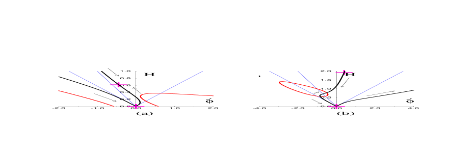
Figure 1: Sample evolutions in the $({\dot{\bar{\phi}}},H)$ phase space. The three blue lines are from left to right, the $(-)$ branch vacuum, the Einstein frame bounce line and the $(+)$ branch vacuum. The $H$ axis is the line of branch change. The black line marked with arrows is the constraint curve (2.3) with the arrows indicating flow direction. Fixed points are marked with magenta crosses and the red curve indicates lines of singularities where the denominator of the expression for $\dot{H}$ and $\ddot{\phi}$ in terms of lower derivatives vanishes. a) The effect of the $O(\alpha^{\prime})$ corrections in [10], $A=-1/2,B=1/2,C=0,D=0$ b) The effect of the correction of [14] $A=-1/2,B=1/2,C=-2,D=1$

Before we look at the consequences of imposing SFD on our sources we look at two examples of explicit evolutions of this type in the $({\dot{\bar{\phi}}},H)$ phase plane. Fig. 1a shows the case $A=-1/2,B=1/2,C=0,D=0$, the case examined in [10] and used as part of the foundation for a model of graceful exit in [9]. The (+) branch vacuum flows into a fixed point located at $(-0.445,0.617)$ after undergoing a branch change. Fig. 1b shows the case $A=-1/2,B=1/2,C=-2,D=1$. This is the form of corrections proposed in [14]. It has the remarkable property of being SFD (indeed $O(d,d)$) invariant, but with the form of the duality (2.16) modified by corrections of order $\alpha^{\prime}$ and with terms of higher order in $\alpha^{\prime}$ truncated. So it does not show the symmetry of (2.16) and furthermore the (+) branch solution flows away from the region of branch change and does not encounter a fixed point.

The important thing to note here is that these corrections are related to the correction (2.7) by a ‘field redefinition’ (check (2.28)) yet show very different behavior. Not only are they different in terms of fixed point behavior, very close to the (+) branch vacuum the curves are turning in opposite directions.

To consider the effects of imposing (2.16) on the correction, we consider a correction with completely general $A,B,C,D$. This adds to the quadratic terms in (2.23) the correction,

$${\cal L}_{c}=\biggl{\{}{{3\,\left(27\,A+8\,B+9\,{C}+27\,{D}\right)\,{{H}^{4}}}\over{2\,{{n}^{3}}}}+{{\left(54\,A+4\,B+9\,{C}+45\,{D}\right)\,{{H}^{3}}\,{\dot{\bar{\phi}}}}\over{{{n}^{3}}}}$$

$$+{{3\,\left(18\,A+{C}+12\,{D}\right)\,{{H}^{2}}\,{{{\dot{\bar{\phi}}}}^{2}}}\over{2\,{{n}^{3}}}}+{{3\,\left(2\,A+{D}\right)\,H\,{{{\dot{\bar{\phi}}}}^{3}}}\over{{{n}^{3}}}}+{{\left(3\,A+{D}\right)\,{{{\dot{\bar{\phi}}}}^{4}}}\over{6\,{{n}^{3}}}}\biggr{\}}.$$ (2.29)

The qualitative question of whether this action has solutions which turn towards the branch change region ($\rho<0$) as in Fig. 1a or away ($\rho>0$) as in Fig. 1b is easily answered by inserting the (+) branch vacuum solution (2.25) into (2.26) (since $\rho$ comes from the variation by $n$, the $\rho$ contribution is proportional to the above form of the action). Numerically, we find the turning direction is determined by the sign of,

$$\rho_{0}=83.5692A+6.3094B+11.1962C+63.1769D.$$ (2.30)

So if $\rho_{0}<0$ we expect the solution to turn towards the branch change and conversely. Also, because the constraint equation contains only terms of degree two and degree four when we restrict ourself to only the $O(\alpha^{\prime})$ corrections, we see the solution can have at most one nonzero intersection with every radial line through the origin. So once it turns one way it will not turn back.

The requirement of SFD symmetry can now be imposed by forcing the action to be SFD invariant. This is done by setting the coefficients of the $H{\dot{\bar{\phi}}}^{3}$ and $H^{3}{\dot{\bar{\phi}}}$ terms to zero, i.e.

$$D = -2A$$

$$C = 4A-{4\over 9}B.$$ (2.31)

We then checked an observation [13] that these corrections fail to satisfy SFD in an anisotropic background, since allowing three different Hubble constants in three directions $H_{x}$, $H_{y}$ and $H_{z}$ will create many more SFD odd terms which must be set to zero. So we simultaneously relaxed the ’no higher derivatives’ conditions, which allows for the nine different tensor structures not related by Bianchi identities shown in (2.13). The equations become enormously more complicated, and since it is not clear which integrations by parts should be performed to exhibit the action in SFD invariant form (if indeed this is possible) we derived the $\bar{\rho}$, $\bar{\lambda}$ and $\bar{\sigma}$ expressions and inspected them for the correct SFD symmetry. We found a two parameter family of corrections which did not break SFD invariance. In terms of the $c$’s of (2.13), the remaining seven coefficients of the SFD invariant corrections can be parameterized in terms of the values of $c_{3}$ and $c_{8}$,

$$c_{0} = 0$$

$$c_{1} = 4c_{3}-c_{8}$$

$$c_{2} = -c_{3}+c_{8}/2$$

$$c_{4} = 4c_{3}-c_{8}$$

$$c_{5} = -2c_{3}$$

$$c_{6} = c_{8}$$

$$c_{7} = -2c_{3}-c_{8}/2.$$ (2.32)

The condition $c_{0}=0$ makes this incompatible with the calculated result (2.7). Further, the only combination of the curvature squared terms not giving rise to higher derivative equations of motion is the Gauss-Bonnet combination, which in turn requires $4c_{0}=4c_{2}=-c_{1}$, so there are no nontrivial members of this family without higher derivative equations of motion.

With these cautions, we still might hope that the family of corrections given by (2.31) might give some clue as to the nature of the correct corrections, and they might indicate that the solutions coming out of the (+) branch vacuum tend to wind up in fixed points. Numerical examinations showed this was not the case. We present a representative family of such evolutions in Fig. 2. Notice the enhanced symmetry over Fig. 1. In Fig. 2a,d we see an attractive and repulsive fixed point on the ${\dot{\bar{\phi}}}$ axis at ${\dot{\bar{\phi}}}$ negative and positive respectively. However they lie on a portion of the constraint curve disconnected from the vacuum part. In Fig. 2b,c the vacuum part of the constraint forms a closed loop, and we could hope it performs the graceful exit on its own. But this loop is cut by the singularity curve where the integration must be halted.

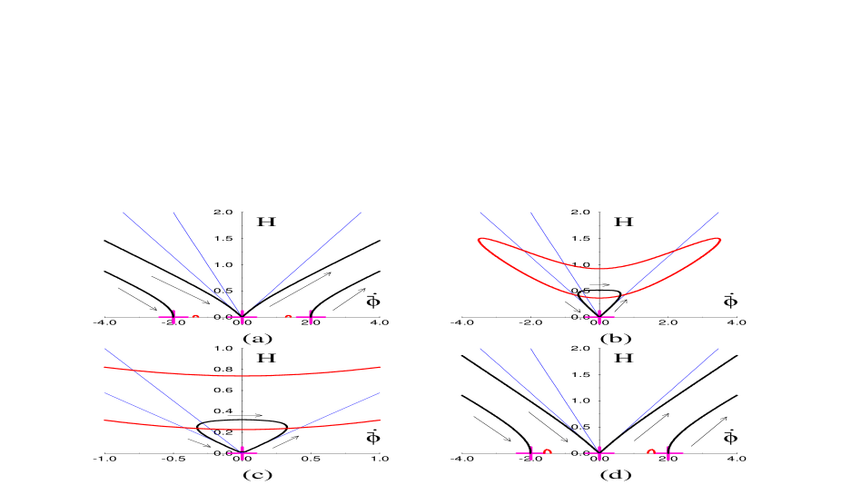
Figure 2: Sample evolutions of corrections constrained by (2.31). Features plotted are as explain in Fig. 1. a) A=1/2, B=1/2. b) A=-1/2, B=1/2. c) A=-1/2, B=-1/2. d) A=1/2, B=-1/2.

2.3 Naive SFD is a Bad Thing

One conclusion might be that this shows that the order $\alpha^{\prime}$ corrections are insufficient to describe the behavior and we need to know the higher order corrections as well. This may be, and indeed the fixed points generally occur at regions of the phase space where the order $\alpha^{\prime}$ corrections are on the same order as the lowest order terms. But there is an even more fundamental obstruction. We will now show that SFD in its naive form (2.16) is generically incompatible with good fixed point behavior.

First of all we note another fundamental symmetry of our equations of motion, time reversal invariance

$${t\rightarrow-t}$$

$${{\dot{\bar{\phi}}}(t)}\rightarrow-{{\dot{\bar{\phi}}}(-t)}$$

$${H(t)\rightarrow-H(-t)}.$$ (2.33)

This tells us that if we have a solution curve in the (${\dot{\bar{\phi}}},H$) plane, we can reflect it through the origin and reverse the time flow to obtain another solution. Putting this together with SFD (2.18), which says we can also reflect solutions across the ${\dot{\bar{\phi}}}$ axis we see solutions can also be reflected across the $H$ axis and time reversed. This in turn tells us the fixed points also occur in pairs reflected across the $H$ axis with one repulsive and one attractive as a result of the time reversal.

Now we repeat an observation [10] that the lowest order action (2.23) is independent of $\beta=\log(a(t))$, and depends only on its derivatives, all explicit $\beta$ dependence having been absorbed into $\bar{\phi}$. We presume this independence will persist in the higher order corrections. This allows us to drop the first term of the variation,

$$\delta\Gamma=\int dte^{-\bar{\phi}}\left[{{\partial{{\cal L}_{eff}}}\over{\partial{\beta}}}{\delta\beta}+{{\partial{{\cal L}_{eff}}}\over{\partial{\dot{\beta}}}}{\delta\dot{\beta}}+{{\partial{{\cal L}_{eff}}}\over{\partial{\ddot{\beta}}}}{\delta\ddot{\beta}}+\ldots\right],$$ (2.34)

so after an integration by parts,

$$\delta\Gamma=\int dt\left[-{{d}\over{dt}}(e^{-\bar{\phi}}{{\partial{{\cal L}_{eff}}}\over{\partial{\dot{\beta}}}})+{{d^{2}}\over{dt^{2}}}(e^{-\bar{\phi}}{{\partial{{\cal L}_{eff}}}\over{\partial{\ddot{\beta}}}})+\ldots\right]\delta\beta=0.$$ (2.35)

Since the quantity in brackets is just proportional to the $\beta$ equation of motion (2.20) with an overall factor of $e^{-\bar{\phi}}$ and it is clearly a total derivative, we can integrate it to get a constant of motion [10],

$$Q=\int dte^{-\bar{\phi}}(\bar{\sigma}-2\dot{H}+2H{\dot{\bar{\phi}}})=e^{-\bar{\phi}}(\bar{\Sigma}-2H),$$ (2.36)

where

$$\bar{\Sigma}(H,{\dot{\bar{\phi}}},\dot{H}.\ldots)=e^{\bar{\phi}}\int dte^{-\bar{\phi}}{\bar{\sigma}}$$ (2.37)

is a function beginning at third degree in derivatives with the $O(\alpha^{\prime})$ corrections. We will find the this conserved constant will allow us to make some statements about the location of fixed points.

Putting $Q=0$ in (2.36) leads to another constraint type equation for the solution, $\bar{\Sigma}-2H=0$. This clearly conflicts at lowest order with the constraint (2.19), so this is not a possibility for solutions originating near the vacuum. Considering a solution approaching a fixed point, we have $\bar{\Sigma}-2H\rightarrow constant$. If ${\dot{\bar{\phi}}}>0$ then clearly the decreasing exponential in (2.36) will force $Q$ to be zero, so the only remaining possibility is ${\dot{\bar{\phi}}}\leq 0$ and $\bar{\Sigma}-2H=0$ in the fixed point. So the diverging exponential is cancelled by the decrease in $\bar{\Sigma}-2H$, but now it would appear we have another algebraic condition to impose on a fixed point, raising the question again of whether fine tuning is necessary to get a fixed point. But we can show this is not the case. The content of the equation (2.20) is equivalent to

$$I_{1}=e^{\bar{\phi}}\left[{{d}\over{dt}}{(e^{-\bar{\phi}}{{\partial{{\cal L}_{eff}}}\over{\partial{H}}})}-{{d^{2}}\over{dt^{2}}}{(e^{-\bar{\phi}}{{\partial{{\cal L}_{eff}}}\over{\partial{\dot{H}}}})}+\ldots\right]=0.$$ (2.38)

The integrated condition $\bar{\Sigma}-2H=0$ which we must enforce at fixed points is proportional to

$$I_{2}=e^{\bar{\phi}}\left[(e^{-\bar{\phi}}{{\partial{{\cal L}_{eff}}}\over{\partial{H}}})-{{d}\over{dt}}{(e^{-\bar{\phi}}{{\partial{{\cal L}_{eff}}}\over{\partial{\dot{H}}}})}+\ldots\right]=0.$$ (2.39)

In a fixed point, the time derivatives of the partial derivatives of $L_{eff}$ vanish, since they are functions of $H$, ${\dot{\bar{\phi}}}$ which are becoming constant and derivatives higher than the first will vanish in a fixed point. So the only non-vanishing parts will come from the time derivatives of the $e^{-\bar{\phi}}$, so $I_{1}=-{\dot{\bar{\phi}}}I_{2}$. So at least in the case where ${\dot{\bar{\phi}}}\neq 0$ in the fixed point, the vanishing of the equation of motion $I_{1}$ implies the vanishing of $\bar{\Sigma}-2H$.

Putting these arguments together shows that fixed points at ${\dot{\bar{\phi}}}<0$ are attractive in the sense that generic ($Q\neq 0$) solutions will flow into them. Conversely, solutions at ${\dot{\bar{\phi}}}>0$ are repulsive in the sense that solutions flow out of them. We have not found an argument classifying the behavior at fixed points at ${\dot{\bar{\phi}}}=0$. In addition, we have the possible existence of $Q=0$ solutions which evade these constraints. We shall have more to say about these when we confront one in section 3.

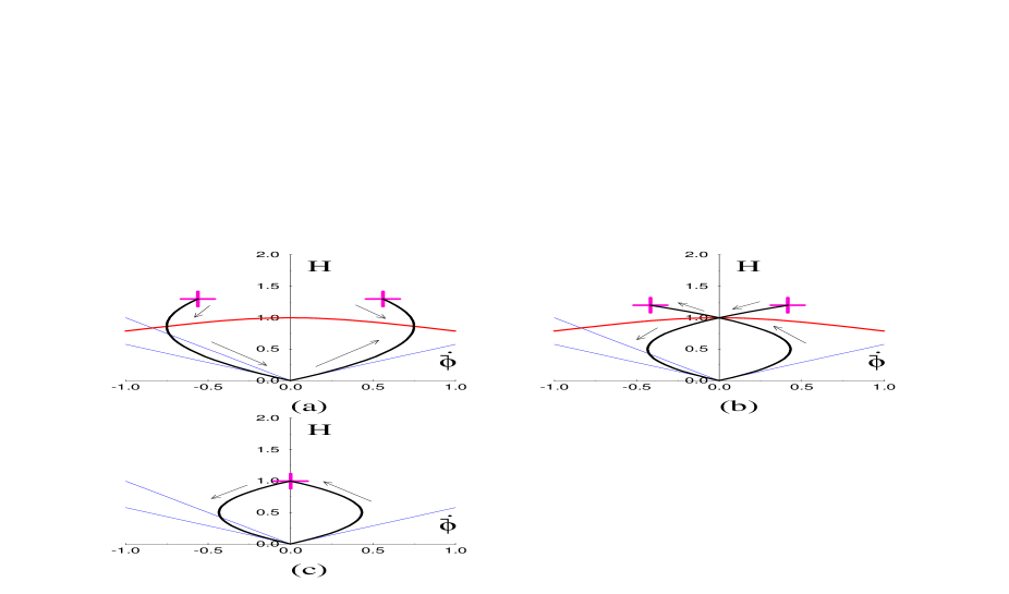
Figure 3: Possible cases of evolution to and from fixed points in the case of a self dual action.

Now we are ready to discuss the possibility of a solution coming out of the $(+)$ branch vacuum and ending in a first fixed point encountered on the constraint curve for an SFD invariant action. Given the symmetries of SFD invariant actions we can draw three possible pictures of such a solution and it’s SFD/time reversed partner, a solution flowing out of a fixed point and into the ($-$) branch vacuum Fig. 3. In Fig. 3a the fixed point is at ${\dot{\bar{\phi}}}\geq 0$. Therefore, as we have argued, this fixed point is repulsive, and a solution will flow out of it rather than in. Given that a solution is also flowing out of the (+) branch vacuum, they must meet at some intermediate point. This point will not be a regular fixed point since we presume the cross marks the first fixed point. The only other possibility is that it is a singularity of the type discussed in [9, 13], which is manifested in the equations of motion by a zero in the denominator of the expression for the highest order derivatives, $\dot{H}$ and ${\ddot{\bar{\phi}}}$ in terms of lower order derivatives, and which we have indicated by drawing such a curve. So this case leads to singular behavior rather than fixed point behavior.

In the second case, Fig. 3b the problem is a little more subtle. Here we have put the first fixed point at ${\dot{\bar{\phi}}}<0$, so it is attractive, but something peculiar is clearly going on where the two solutions cross. We have two solutions leaving the same (${\dot{\bar{\phi}}},H$) point, when we would expect that the value of ${\dot{\bar{\phi}}}$ and $H$ would uniquely specify initial conditions. This is because first, we have presumed that equations are at most second order in derivatives. Second, the variables $a(t)$ and $\phi(t)$ do not appear explicitly in the equations of motion. In fact, this situation is the same as the singularity in the first case. The expressions for $\dot{H}$ and ${\ddot{\bar{\phi}}}$ take the indeterminate form $0/0$ at this point. So the curve corresponding to the vanishing of the denominators of these expressions also passes through this point, and higher derivatives go to infinity in the neighborhood of such points. Numerical simulations are wildly unstable passing through there, and we regard it as physically unstable as well.

It might be objected that this looks like the behavior at the origin. This is indeed possible if this crossing point is also a ${\dot{\bar{\phi}}}=0$ fixed point, like the origin. In this case the solutions don’t actually cross, but just asymptotically approach this point. This is the boundary behavior of both of the previous cases when the fixed points are allowed to approach each other. This is an interesting place for a fixed point, it is mapped into itself by a combination of SFD and time reversal and so is both a $(+)$ and $(-)$ branch solution simultaneously.

We now discuss briefly the possiblity of placing the fixed point at ${\dot{\bar{\phi}}}=0$, Fig. 3c, the only possibility that would allow us to retain both simple SFD (2.16) and good fixed point behavior. To do this we need to examine the equations of motion with all derivatives higher than the first set to zero, and with ${\dot{\bar{\phi}}}=0$. A little thought will show that the only terms in the action that can contribute to these reduced eoms are

$$\int dte^{-\bar{\phi}}({{3H^{2}}\over{n}}+c_{1}{{H^{4}}\over{n^{3}}}+c_{2}{{H^{6}}\over{n^{5}}}+\ldots),$$ (2.40)

where the dependence on $n(t)$, the lapse factor, is dictated by time reparameterization invariance. Performing the variation with respect to $n$, as in (2.19), and with respect $\bar{\phi}$, as in (2.21), and setting $n=1$, we get the following,

$$3H^{2}+3c_{1}H^{4}+5c_{2}H^{6}+\ldots = 0$$ (2.41)

$$3H^{2}+c_{1}H^{4}+c_{2}H^{6}+\ldots = 0.$$ (2.42)

So we see there are no non-trivial ${\dot{\bar{\phi}}}=0$ fixed points at order $\alpha^{\prime}$ (allowing us at most the power $H^{4}$). At $O(\alpha^{\prime 2})$ it would seem to be possible. But we have not classified covariant tensor structures at this order and have no results comparable to (2.7). Even so we have tried to introduce SFD invariant corrections of the form expected at $O(\alpha^{\prime 2})$ and while we can position a fixed point at ${\dot{\bar{\phi}}}=0$ we have found no cases where it well behaved and connected to the vacuum. This should be expected, since this case be looked at as a limiting case of the two previous cases, where the action is manipulated to allow the two fixed point to approach each other. Since the previous cases exhibit pathologies, they should probably be expected to persist in the limit, but we don’t regard this as a rigorous argument.

To summarize, we have shown that good fixed point behavior and SFD with eoms containing derivatives at most of order two require fixed points at ${\dot{\bar{\phi}}}=0$, which in turn seems to be difficult to achieve.

On the other hand, it is not difficult to find good fixed point behavior (as in [10]) if SFD is broken. So to sum up, perversely we have the situation where imposing a string theoretical notion (SFD) on possible classical corrections seems to create difficulties for achieving another string theory notion, that finite size string effects will saturate curvature growth.

There are several different conclusions to be drawn. One is simply to accept these conclusions and retain faith in both the simplest form of SFD and curvature saturation. Perhaps if and when we can determine the correction to all orders it will exactly solve (2.42) allowing a ${\dot{\bar{\phi}}}=0$ fixed point and shed pathologies. A second is the suggestion of [13], that we must consider the contribution of the massive string modes, which may help to saturate curvature growth. A third direction lies in a modification of the form of duality. As discussed in [16], the source of SFD is a classical symmetry involving the exchange of winding and momentum modes on the string world sheet, so at this level the dilaton does not participate in SFD at all, since the dilaton only enters the theory at the quantum level. The non-trivial transformation of the dilaton comes at the level of the effective action, where we are working with ‘renormalized’ fields, which mix the dilaton with the scale factor. Working to higher orders in the corrections, one should expect additional renormalizations and hence corrections to the form of SFD. This expectation was exploited in [14] to actually fix the form of the action and correction at $O(\alpha^{\prime})$, based on correct order by order cancellation of non-$O(d,d)$ invariant terms. As we have seen, this form of correction does not lead to fixed point behavior (Fig. 1b). But as we will see in the next section, it is close to the region of parameter space that admits fixed points without SFD. Further, considering (2.21) we see that the source $\bar{\lambda}$ has to be at least of the same order as $H^{2}$ or ${\dot{\bar{\phi}}}^{2}$, so the corrections cannot be small in a fixed point. This suggests that rather than simply conclude SFD works against fixed point behavior, we will require more knowledge of higher order corrections and/or of the form scale factor duality takes in the higher order effective action.

2.4 The Distribution of Fixed Points

Since at this level SFD does not lead to interesting conclusions regarding the fixed point behavior, we return to the general form of corrections (2.26) and simply ask the question, what region of the ($A,B,C,D$) parameter space for the corrections leads to good fixed point behavior and where are the fixed points located? Since this is a four dimensional space we also impose the conditions (2.27) and (2.28), reducing us to a two parameter space ($A,D$). To find these fixed points one should be careful not only to check algebraically that the fixed points exist but that they are reachable from solutions beginning near the (+) branch vacuum. To do this we run numerical integrations from initial conditions near the (+) branch vacuum and examine the solutions for fixed point behavior at late time. In Fig. 4a we have placed a dot on a grid where an ($A,D$) selection leaves to good fixed point behavior. We have also marked the line corresponding to the condition (2.30). As expected, there is no good fixed point behavior to the right of this line, since the solutions initially veer from the vacuum away from branch change, hence towards ${\dot{\bar{\phi}}}>0$ where we find only unstable fixed points. But good fixed point behavior almost saturates the region to the left.

We have also marked with crosses the corrections corresponding to the $\alpha^{\prime}$ corrections used to produce fixed point behavior in [10, 7, 9] inside of the region of good fixed parameters, and also the parameters corresponding to the corrections of [14], whose evolution is plotted in Fig. 1b, which lies outside of this region. This form of the corrections is perhaps the best motivated form of the corrections, coming from an exact but truncated form of $O(\alpha^{\prime})$ modified duality. It is discouraging that it is outside the region of good fixed point behavior, but encouraging to note that it is not far away, suggesting higher order corrections could easily modify it’s behavior.

In Fig. 4b we plot the locations of the resulting fixed points in the (${\dot{\bar{\phi}}},H$) plane and the location of the fixed point used in [10, 7, 9]. We find that the good fixed points are all located in a wedge bounded by ${\dot{\bar{\phi}}}\leq 0$ and $H\geq-{\dot{\bar{\phi}}}$. The first boundary is easy to understand, since we have just shown that the stable fixed points must be located at ${\dot{\bar{\phi}}}\leq 0$. The second is harder to understand. But we do observe that the line $H=-{\dot{\bar{\phi}}}$ is just the line where the scale factor undergoes a bounce in the Einstein frame, and producing this bounce requires the sources to violate the Null Energy Condition ($\rho+p\geq 0$) [7, 9]. As these sources represent classical string corrections which are not expected to violate NEC, it is possible these constraints contain part of that condition.

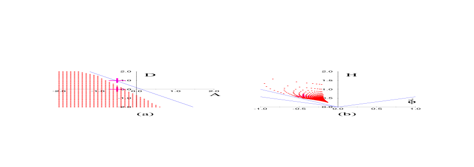
Figure 4: a) The distribution of coefficients leading to good fixed point behavior in the ($A,D$) plane. $C$ and $D$ are chosen to fit the constraints (2.27) and (2.28). The line plotted is the condition of (2.30), to the right of this line solutions turn away from branch change and are not expected to lead to good fixed point behavior. The crosses marks the location of the corrections figured in Fig. 1. b) The location in the (${\dot{\bar{\phi}}},H$) plane of the resulting good fixed points. The cross marks the location of the fixed point shown in Fig. 1a.

3 Conformal Field Theories

We have seen that investigations of the behavior of solutions including only $O(\alpha^{\prime})$ corrections leads to, at best, ambiguous conclusions about their fixed point behavior. Since the classical equations of motion for the background fields of the string are derived from the requirement that they preserve conformal invariance on the string worldsheet [17], directly constructing a conformally invariant background would give a solution to all orders in $\alpha^{\prime}$, even without knowledge of the form of the corrections. While there is a large literature of exact cosmological solutions [18] (coming, for example, from gauged WZW models), all exhibit either extreme anisotropy or are supported by other fields in addition to the graviton and the dilaton. So they are not particularly relevent to this scenario. We will take a more naive and non-rigorous approach to constructing a background which we hope will at least have properties in common with a conformally invariant background.

Recalling the classical action for the bosonic string,

$$S=\frac{1}{4\pi\alpha^{\prime}}\int{d\tau}{d\sigma}\sqrt{\gamma}\left[\gamma^{\alpha\beta}G_{\mu\nu}(X)\partial_{\alpha}X^{\mu}\partial_{\beta}X^{\nu}+R^{(2)}(X)\Phi(X)\right],$$ (3.1)

where $\tau$ and $\sigma$ are coordinates and $\gamma$ is the metric on the string worldsheet, $X^{\mu}$ and $G^{\mu\nu}$ are the spacetime coordinates and metric, $R^{(2)}$ the worldsheet curvature and $\Phi$ is the dilaton. With $G^{\mu\nu}=\eta^{\mu\nu}=(-,+,+,\ldots)$ this leads to a conformally invariant theory in critical dimensions where the reparameterization ghosts cancel the contribution to the central charge of the bosonic fields $X^{\mu}$. In the following we ignore issues related to the central charge of the model, expecting it can also be cancelled by the addition of other sources that are ‘inert’, in the sense of not affecting the other conclusions we draw. We introduce a nontrivial background in the above by assuming

$$\Phi(X)=PX^{0}=Pt,$$ (3.2)

where P is a constant, giving a dilaton varying linearly in time. We also add to the flat space action ((3.1) with $G^{\mu\nu}=\eta^{\mu\nu}$) the term,

$${\cal O}_{K}(z,\bar{z})=\sum\limits_{i>0}\gamma^{\alpha\beta}e^{2KX^{0}}\partial_{\alpha}X^{i}(z,\bar{z})\partial_{\beta}X^{i}(z,\bar{z}).$$ (3.3)

This leads to an action with a total background metric of FRW form with $a(t)=\sqrt{1+e^{2Kt}}$, interpolating between flat space and a de-Sitter form like our expected fixed point solutions. But we will need to insure that the addition of (3.3) to the action hasn’t spoiled conformal invariance.

A first step in this direction is to check that quantum effects do not change the classical scaling dimension of (3.3). A standard framework for doing this falls under the name of conformal perturbation theory (see, for example, [19]). The energy momentum tensor for the flat space action (3.1) with the linear dilaton ansatz is,

$$T_{zz}=-\frac{1}{2}\left(\partial_{z}X^{0}\partial_{z}X^{0}-\sum\limits_{i>0}\partial_{z}X^{i}\partial_{z}X^{i}+P\,\partial^{2}_{z}X^{0}\right),$$ (3.4)

where we have used conformal invariance to put the world-sheet metric into the conformal gauge ($\gamma_{z\bar{z}}=\gamma_{\bar{z}z}=1,\gamma_{zz}=\gamma_{\bar{z}\bar{z}}=0$). There are also exactly parallel formulae for the anti-holomorphic parts ($\bar{z}$), which decouple from the holomorphic parts.

The requirement that ${\cal O}_{K}$ transform as a conformal tensor is just,

$${\cal O}_{K}(z,\bar{z})\rightarrow\left({{\partial{f}}\over{\partial{z}}}\right)^{h}\left({{\partial{\bar{f}}}\over{\partial{\bar{z}}}}\right)^{\bar{h}}{\cal O}_{K}(f(z),\bar{f}(\bar{z})).$$ (3.5)

Since we require the action to be an invariant, we want $h=\bar{h}=1$ to offset the scaling of the integration measure ${dz}{d\bar{z}}$. Since $T_{zz}$ is the generator of conformal transformations, it can be shown that (3.5) requires the following singularity structure in the operator product expansion,

$$T_{zz}(z){\cal O}_{K}(w,\bar{w})=\frac{h}{(z-w)^{2}}{\cal O}_{K}(w,\bar{w})+\frac{1}{(z-w)}\partial_{w}{\cal O}_{K}(w,\bar{w})+{\rm non-singular}.$$ (3.6)

As usual this can be related to a normal ordered product by contracting operators as specified by Wick’s theorem and using the following ‘mnemonic’ for the propagators,

$$<X^{\mu}(z)X^{\nu}(w)>=\eta^{\mu\nu}\log(z-w).$$ (3.7)

This is a mnemonic in the sense that it correctly represents the short distance behavior of the propagator and the operators are to be regarded as normal ordered in the sense that we do not include divergent contractions of operators with the same argument.

So the expression corresponding to the holomorphic part of the $i^{th}$ component of the left hand side of (3.6) becomes,

$$-\frac{1}{2}\left(\partial_{z}X^{0}(z)\partial_{z}X^{0}(z)-\partial_{z}X^{i}(z)\partial_{z}X^{i}(z)+P\,\partial^{2}_{z}X^{0}(z)\right)e^{2KX^{0}(w)}\partial_{w}X^{i}(w)$$ (3.8)

The contractions are easily carried out because of the simple behavior of the exponential under contractions. The result is,

$$\frac{e^{2KX^{0}(w)}}{(z-w)^{2}}\left(\partial_{z}X^{i}(z)-K(P+2K)\partial_{w}X^{i}(w)\right)+\frac{e^{2KX^{0}(w)}}{(z-w)}2K\partial_{z}X^{0}(z)\partial_{w}X^{i}(w)$$ (3.9)

If we insert the Taylor expansion, $\partial_{z}X^{\mu}(z)=\partial_{w}X^{\mu}(w)+(z-w)\partial^{2}_{w}X^{\mu}(w)\ldots$, we recognize this as,

$$\frac{(1-K(P+2K)){\cal O}_{K}(w)}{(z-w)^{2}}+\frac{\partial_{w}{\cal O}_{K}(w)}{(z-w)}+{\rm non-singular}.$$ (3.10)

Comparing this with (3.6) we identify ${\cal O}_{K}$ as a conformal tensor of dimension $1-K(P+2K)$, so we can nontrivially satisfy the requirements of conformal invariance by setting $P=-2K$.

Next to make contact with $\phi$, the dilaton in our effective action, we compare our equations of motion with those of [17]. We conclude that $2\Phi=\phi$. Reading off the space-time metric and dilaton,

$$\phi(t)=2Pt$$

$$P=-2K$$

$$a(t)=\sqrt{1+e^{2Kt}}$$

$$H(t)=\frac{K}{1+e^{-2Kt}}$$

$${\dot{\bar{\phi}}}(t)=-4K-3H(t)$$ (3.11)

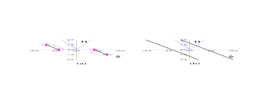
Figure 5: a) The CFT trajectory, K=1, on the left and its time reversed partner on the right, with beginning and ending fixed points marked. b) The CFT trajectory extended to include all of the fixed points allowed by the equations of motion from an effective action.

A sample of such an evolution is given in Fig. 5a. It is unusual in light of our previous results. Its fixed points sit beyond the line $H=-{\dot{\bar{\phi}}}$ where the Einstein frame bounce requires NEC violation, so we perhaps should not expect solutions originating near the vacuum to flow into this fixed point. Secondly, it is flowing out of a fixed point at ${\dot{\bar{\phi}}}<0$, the opposite of the expected behavior, as we discussed in section 2.3. So we expect that if it is in fact a solution to an effective action, we will find it is a $Q=0$ solution.

To try to understand the implications of such a solution on the form of the effective action we construct the most general effective action not involving higher derivatives and attempt to fix the coefficients by demanding this solution solve the eoms. We took the action to be of the form,

$$\Gamma=\int dte^{-\bar{\phi}}{\cal L}(H(t),{\dot{\bar{\phi}}}(t),n(t))$$

$${\cal L}=\sum\limits_{n,i}c_{n,i}H(t)^{i}{\dot{\bar{\phi}}}(t)^{n-i}/n(t)^{n-1},$$ (3.12)

where the sum is over even values of n. As before, the power of the lapse factor $n(t)$ is dictated by time reparametrization invariance. This is the most general action that can be produced by covariant tensor corrections that do not introduce higher derivatives. We can explicitly display the equations of motion in terms of ${\cal L}$.

$${{\partial{{\cal L}}}\over{\partial{n}}}=0$$ (3.13)

$${{\partial{{}^{2}}{{\cal L}}}\over{\partial{H}{{}^{2}}}}\dot{H}+{{\partial{{}^{2}}{{\cal L}}}\over{\partial{H}\partial{{\dot{\bar{\phi}}}}}}{\ddot{\bar{\phi}}}-{\dot{\bar{\phi}}}{{\partial{{\cal L}}}\over{\partial{H}}}=0$$ (3.14)

$${{\partial{{}^{2}}{{\cal L}}}\over{\partial{H}\partial{{\dot{\bar{\phi}}}}}}\dot{H}+{{\partial{{}^{2}}{{\cal L}}}\over{\partial{{\dot{\bar{\phi}}}}{{}^{2}}}}{\ddot{\bar{\phi}}}-{\dot{\bar{\phi}}}{{\partial{{\cal L}}}\over{\partial{{\dot{\bar{\phi}}}}}}+{\cal L}=0.$$ (3.15)

We then fix $c_{2,2}=3$, $c_{2,1}=0$ and $c_{2,0}=-1$ reflecting our knowledge of the lowest order action and add a finite number of terms with even $n$, insert (3.11) into the resulting equations of motion and attempt to solve the resulting linear system for the coefficients $c_{n,i}$. At the level $n=4$ we find no solutions. But adding the $n=6$ terms gives a one parameter family of solutions and adding $n=8$ an even larger family of solutions. And this is in spite of the fact we get many more equations than free parameters.

A hopeful conclusion is that we have done something right, and the form of (3.11) is well suited to solution by relatively lower orders in expected forms of the effective action. But closer examination of the resulting equations of motion showed that when the initial condition appropriate to the solution (3.11) are inserted the resulting equations become degenerate, and we don’t have enough dynamical equations to reconstruct (3.11). In particular, both of the dynamical equations (3.14) and (3.15) become ${\ddot{\bar{\phi}}}(t)=-3\dot{H}(t)$.

Again a hopeful conclusion is that this is evidence for the special nature of (3.11). But in fact this can be seen to be true of any $Q=0$ solution. Referring to (2.35), we see that the conserved quantity for our action ansatz can be written,

$$Q=e^{-\bar{\phi}}{{\partial{{\cal L}}}\over{\partial{H}}},$$ (3.16)

so the $Q=0$ condition becomes ${{\partial{{\cal L}}}\over{\partial{H}}}=0$. So the lower order part in (3.14) becomes identically zero. The lower order part in the second dynamical equation is, in terms of the action (we also set $n(t)=1$),

$${\cal L}-{\dot{\bar{\phi}}}{{\partial{{\cal L}}}\over{\partial{{\dot{\bar{\phi}}}}}}=\sum\limits_{n,i}c_{n,i}H(t)^{i}{\dot{\bar{\phi}}}(t)^{n-i}-\sum\limits_{n,i}(n-i)c_{n,i}H(t)^{i}{\dot{\bar{\phi}}}(t)^{n-i}.$$ (3.17)

Combining this with (3.13),

$$\sum\limits_{n,i}(n-1)c_{n,i}H(t)^{i}{\dot{\bar{\phi}}}(t)^{n-i}=0,$$ (3.18)

we see,

$${\cal L}-{\dot{\bar{\phi}}}{{\partial{{\cal L}}}\over{\partial{{\dot{\bar{\phi}}}}}}=\sum\limits_{n,i}ic_{n,i}H(t)^{i}{\dot{\bar{\phi}}}(t)^{n-i}=H{{\partial{{\cal L}}}\over{\partial{H}}}.$$ (3.19)

So, in fact, the $Q=0$ condition, ${{\partial{{\cal L}}}\over{\partial{H}}}=0$ causes the dynamical equations to become homogeneous equations in the higher derivatives. Since a homogeneous system does not have a unique non-zero solution, we have lost the ability to recover the time dependence of (3.11) from the equations of motion.

While this disturbing and unexpected, it has another interesting implication. Any point on the trajectory can be regarded as a fixed point, since $({\dot{\bar{\phi}}},H)=constant$ trivially satisfies the eoms (3.14) and (3.15) by virtue of the vanishing of the lower derivative contributions. In other words because of this degeneracy of the eoms, instead of having isolated fixed points we have curves of fixed points.

Furthermore, although the CFT trajectory occupies only a finite segment in the $({\dot{\bar{\phi}}},H)$ phase space, looking at the situation from the view point of the eoms this is only part of the story. Consider the equation (3.13) which is just a polynomial in ${\dot{\bar{\phi}}}$ and $H$. Since it vanishes on the segment defined by (3.11) it follows that (3.13) contains a linear factor which is just the equation defining the segment, explicitly ${\dot{\bar{\phi}}}+3H(t)+4K$. Since this linear factor vanishes on the entire infinite line containing the segment we find this constrain equation is valid on the entire line. Similarly, since the quantity ${{\partial{{\cal L}}}\over{\partial{H}}}=0$ must be satisfied on the segment it must also be satisfied on the entire line. So the previous arguments can be seen to hold on the entire line. So we have, in fact, have an infinite line of fixed points.

Now consider the time reversed solution, clearly it also a $Q=0$ trajectory, since when ${\dot{\bar{\phi}}}\rightarrow-{\dot{\bar{\phi}}}$ and $H(t)\rightarrow-H(t)$ we have ${{\partial{{\cal L}}}\over{\partial{H}}}\rightarrow-{{\partial{{\cal L}}}\over{\partial{H}}}$ since it only contains terms of odd degree. All of the foregoing apply to it also, so it can also be extended to an infinite line of fixed points. We have illustrated these extended lines in Fig. 5b.

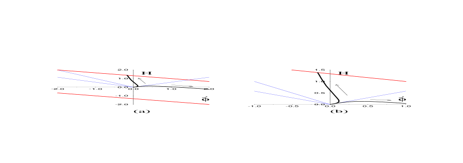
Figure 6: a) Trajectories coming from the (+) vacuum, K=1, for effective actions that contain (3.11) as a solution. The red lines are the lines of fixed points created by (3.11) (below) and its time reversed partner (above). b) A closer view of a) showing the solution going to a fixed point on the line created by the time reversed partner of (3.11).

Returning our attention to the solution coming from the (+) branch vacuum where the equations of motion are generically nonsingular, we observe that it is between two lines of fixed points. The points at ${\dot{\bar{\phi}}}>0$ are repulsive and the solution cannot flow into them or cross them. But those at ${\dot{\bar{\phi}}}<0$ are attractive and make a large target of future attractors. So the (+) branch solution may either flow to infinity or singularity between the lines or flow to one of the ${\dot{\bar{\phi}}}<0$ fixed points. The choice between these alternatives depends on the exact form of the effective action. As we have stated, requiring (3.11) to be a solution of the effective action to a given order does not fix the coefficients in the effective action but only constrains them. We illustrate the situation in Fig. 6. Here we have fitted an effective action of order $O(\alpha^{\prime 2})$ to the CFT solution, which leaves us with one free parameter. Setting this parameter to two different values allows us to exhibit these two different types of behavior by numerically integrating the (+) branch vacuum solution. While we find that the solutions are not compelled to flow to the fixed points, such behavior seems to occur over a large portion of the parameter space.

While these observations depend on the exact nature of the CFT solution and we should not expect it to be exact as we are working in conformal perturbation theory, we remark that much of the previous argument can be applied to a solution which only qualitatively resembles the CFT solution. The fact it is a $Q=0$ solution is necessary only because it exits from a ${\dot{\bar{\phi}}}<0$ fixed point. As this is the most reliable perturbative regime (as $t\rightarrow-\infty$), this is perhaps reasonable. And while we lose the exact factorization arguments, a line of zeros of a polynomial expression does not simply terminate at a point as the CFT solution does. So we should expect that the resulting curve of fixed points can again be extended.

We have made use of the time reversed CFT solution but have made no mention of SFD. We expect imposing the naive form of SFD will only eliminate good fixed point behavior, as we have argued, so we do not base any arguments on it. We do expect that the form of the action should reflect some form of SFD, but without knowing something of its nature it is difficult to be exact. Since the naive SFD partner of the CFT solution flows out of a ${\dot{\bar{\phi}}}<0$ fixed point we should expect the exact SFD partner does as well, making it in turn a $Q=0$ solution and a line of fixed points. So we may find other walls of fixed points around as well, compelling the solution coming out of the (+) vacuum to have good fixed point behavior.

4 Conclusions

We have seen that the known information about the nature of the $O(\alpha^{\prime})$ corrections to the effective action coming from string theory are insufficient to decide whether inflationary branch used in the pre-big-bang scenario exhibits curvature saturation by flowing into a fixed point. Attempts to use SFD to further constrain the action finally lead an exact statement independent of the order of correction that naive SFD simply works against this behavior. However we have also observed that naive SFD simply cannot be implemented at $O(\alpha^{\prime})$ in the general anisotropic case and we concur with other work suggesting that SFD itself must receive higher order corrections.

We have also scanned the parameter space of possible forms of corrections and have determined that good fixed point behavior, while not universal, does occupy a large region of this parameter space. Finally, we have attempted to construct a plausible approximation to a conformally exact solution and discovered that independent of its exact form, a generically similar solution forces the equations of motion to a corresponding action to exhibit a degeneracy which forces the existence of continuous lines of fixed points. These fixed points can in turn powerfully constraint the possible evolution of the (+) inflationary branch, opening the possibility that deeper knowledge of some conformally exact solutions may be enough to settle the question of whether string theory predicts curvature saturation for the inflationary scenario of string cosmology.

Acknowledgment

This research is supported in part by the Israel Science Foundation administered by the Israel Academy of Sciences and Humanities.

References

- [1] S.W. Hawking and R. Penrose, Proc. Roy. Soc. Lond. A314 (1970) 529.
-
[2]
P. Binetruy and M-K Gaillard, Phys. Rev. D32 (1986) 3069;
D.G. Boulware and S. Deser, Phys. Lett. B175 (1986) 409;
S. Kalara and K.A. Olive, Phys. Lett. B218 (1989) 148;
R. Brustein and P. Steinhardt, Phys. Lett. B302 (1993) 196. - [3] G. Veneziano, Phys. Lett. B265 (1991) 287.
- [4] M. Gasperini and G. Veneziano, Astropart. Phys. 1 (1993) 317.
-
[5]
R. Brustein, M. Gasperini, M. Giovannini and G. Veneziano,
Phys. Lett. B361 (1995) 45;
M. Gasperini, M. Giovannini and G. Veneziano, Phys. Rev. Lett. 75 (1995) 3796;
D. Lemoine and M. Lemoine, Phys. Rev. D52 (1995) 1955;
R. Durrer, M. Gasperini, M. Sakellariadou and G. Veneziano, Phys. Lett. B436 (1998) 66;
R. Brustein and M. Hadad, hep-ph/9810526. -
[6]
T. Damour and A.M. Polyakov, Nucl. Phys. B423 (1994) 532;
B.A. Campbell and K.A. Olive, Phys. Lett. B345 (1995) 429. - [7] R. Brustein and R. Madden, Phys. Lett. B410 (1997) 110.
-
[8]
N. Kaloper, R. Madden and K.A. Olive, Nucl. Phys. B452 (1995) 677;
R. Brustein and G. Veneziano, Phys. Lett. B329 (1994) 429. - [9] R. Brustein and R. Madden, Phys. Rev. D57 (1998) 712.
- [10] M. Gasperini, M. Maggiore and G. Veneziano, Nucl. Phys. B494 (1997) 315.
- [11] R.R. Metsaev and A.A. Tseytlin, Nucl. Phys. B293 (1987) 385.
- [12] K. Forger, B. Ovrut, S. Theisen and D. Waldram Phys. Lett. B388 (1996) 512.
- [13] M. Maggiore, Nucl. Phys. B525, 413 (1997).
-
[14]
K.A. Meissner, Phys. Lett. B392 (1997) 298;
N. Kaloper, K.A. Meissner, Phys. Rev. D56 (1997) 7940. - [15] E. Flanagan and R. Wald, Phys. Rev. D54 (1996) 6233;
-
[16]
K.A. Meissner and G. Veneziano, Phys. Lett. B267 (1991) 33;
K.A. Meissner and G. Veneziano, Mod. Phys. Lett. A6 (1991) 3397;
A. Sen, Phys. Lett. B271 (1991) 295;
M. Gasperini and G. Veneziano, Phys. Lett. B277 (1992) 256. -
[17]
C. Callan, D. Friedan, E. Martinec and M. Perry Nucl. Phys. B262 (1985) 593;
E. Fradkin and A. Tseytlin, Phys. Lett. B158 (1985) 316; Nucl. Phys. B261 (1985) 1. - [18] A.A. Tseytlin, Class. Quant. Grav. 12 (1995) 2365-2410.
- [19] E. Kiritsis, hep-th/9709062, to be published by Leuven University Press.