Theoretical Physics Institute
University of Minnesota

TPI-MINN-98/29-T

UMN-TH-1734-98

December 1998

On intersection of domain walls in a supersymmetric model

S.V. Troitsky
Institute for Nuclear Research of the Russian Academy of Sciences,

60th October Anniversary Prospect 7a, Moscow 117312

and

M.B. Voloshin
Theoretical Physics Institute, University of Minnesota, Minneapolis, MN 55455

and

Institute of Theoretical and Experimental Physics, Moscow, 117259

We consider a classical field configuration, corresponding to intersection of two domain walls in a supersymmetric model, where the field profile for two parallel walls at a finite separation is known explicitly. An approximation to the solution for intersecting walls is constructed for a small angle at the intersection. We find a finite effective length of the intersection region and also an energy, associated with the intersection.

1 Introduction

The problem of domain walls has a long history both in its general field aspect [1] and in a possible relevance to cosmology [2]. Recently the interest to properties of domain walls has been given a new boost in supersymmetric models, which naturally possess several degenerate vacua, thus allowing for a multitude [3] of domain wall type configurations interpolating between those vacua. Furthermore it has been realised [4, 5] that at least some of these walls have rather distinct properties under supersymmetry and in fact their field profiles satisfy first order differential equations in analogy with the Bogomol’nyi - Prasad - Sommerfeld (BPS) equations [6]. For this reason such configurations are called “BPS-saturated walls”, or “BPS walls”. It was also noticed [7] that, quite typically, there may exist a continuous set of the BPS walls, all degenerate in energy, interpolating between the same pair of vacua. A further analysis [8] of such set in a specific model revealed that the solutions in the set can be interpreted as two elementary BPS walls parallel to each other at a finite separation, the distance between the walls being the continuous parameter labeling the solutions. Since all the configurations in the set have the same energy, equal to the sum of the energies of the elementary walls, one encounters here a remarkable situation where there is no ‘potential’ interaction between the elementary walls. (This property is protected by supersymmetry and holds in all orders of perturbation theory.)

The existence of multiple vacua in supersymmetric models naturally invites a consideration of more complicated field configurations, than just two vacua separated by a domain wall, namely those with co-existing multiple domains of different degenerate vacua [3]. This leads to the problem of intersecting domain walls. It should be noted, that by far not every conceivable configuration of domains is stable, e.g. any intersection of domain walls in a one-field theory is unstable, and the conditions for stability of the intersections of the walls in multiple-field theories[3] generally allow only a well defined set of intersection angles, depending on relation between the energy densities of the intersecting walls. As is discussed further in this paper, for the elementary BPS walls, considered in [8], i.e. non-interacting in the parallel configuration (zero intersection angle $\beta$), at least a finite range of values for $\beta$, including $\beta=0$, is allowed by the stability conditions for a quadruple intersection, shown in Fig.1. When viewed as an intersection of world surfaces of the walls in the space-time, rather than as a static spatial configuration, the intersection describes scattering of moving walls, and in the case of a collision of spatially parallel walls (or kinks in a (1+1) dimensional model) the angle $\beta$ translates into $\beta=v/c$ with $v$ being the relative velocity of the walls, for small $\beta$, i.e. for non-relativistic collisions. The purpose of the present paper is a more detailed study of the field profile for the intersection configuration of such type. We consider here the same supersymmetric model as in Ref.[8] and use the explicit solution for parallel walls, found there, to construct an approximation to the classical field profile for intersecting walls, which is valid to the first order in $\beta$ for small $\beta$. This approximation gives the energy of the static field configuration up to $\beta^{2}$ inclusive, while for the case of collision of the walls the corresponding result is obviously the action for the collision “trajectory”.

Figure 1: Quadruple vertex for four different vacuum domains

Our main findings are as follows. There exists a well defined gap $\Delta x$ between the vertices of pairwise ‘meet’ of the walls, so that a more detailed picture of the intersection looks as shown in actual detail in Fig.3 further in the paper. In the collision kinematics this gap is in time and corresponds to a finite time delay in the scattering process. This classical quantity clearly can also be translated into a phase shift in a quantum mechanical description of the scattering. The gap depends on the intersection angle, and is given by

$$\Delta x={1\over\beta}\,{\ell_{0}\over m}~{},$$ (1)

where $m$ is a mass parameter for the masses of quanta in the model, and $\ell_{0}$ is a dimensionless constant, depending on the ratio of the coupling constants in the model. We also find that there is a finite angle-dependent energy (in the static configuration) associated with the intersection:

$$\varepsilon=\beta\,\mu\,{\ell_{0}\over m}~{},$$ (2)

where $\mu$ is the energy density of each of the elementary walls. Naturally, in a (3+1) dimensional theory $\varepsilon$ is in fact the energy per unit length of the intersection, while in a (2+1) dimensional case it is an energy localized at the intersection. In a (1+1) dimensional model only the collision kinematics (for two elementary kinks) is possible, thus $\varepsilon$ has the meaning of a finite action (phase shift) associated with the collision. We believe that the equations (1) and (2) are quite general at small $\beta$, and the only model dependence is encoded in the dimensionless quantity $\ell_{0}$.

The rest of the paper is organized as follows. In Section 2 we present the supersymmetric model under consideration and describe the solutions for the BPS walls. In Section 3 we consider intersecting domain walls within an Ansatz allowing us to construct the field profiles in the limit of small intersection angle, and we find the characteristics of the intersection. In Section 4 we discuss applicability of the findings of this paper when some of the restrictions, assumed here, are relaxed.

2 Domain walls in a SUSY model

The specific SUSY model under consideration is that of two chiral superfields $\Phi$ and $X$ with the superpotential

$$W(\Phi,\,X)={m^{2}\over\lambda}\,\Phi-{1\over 3}\,\lambda\,\Phi^{3}-\alpha\,\Phi\,X^{2}\,.$$ (3)

Here $m$ is a mass parameter and $\lambda$ and $\alpha$ are coupling constants. The phases of the fields and of the $W$ are assumed to be adjusted in such a way that all the parameters are real and positive, and the lowest components of the superfields $\Phi$ and $X$ are denoted correspondingly as $\phi$ and $\chi$ throughout this paper. The model has the $Z_{2}\times Z_{2}$ symmetry under independent flip of the sign of either of the fields: $\Phi\to-\Phi$, $X\to-X$. The vacuum states in this model are found as stationary points of the superpotential function (3): $\partial W(\phi,\,\chi)/\partial\phi=0$ and $\partial W(\phi,\,\chi)/\partial\chi=0$, and are located at $\phi=\pm m/\lambda$, $\chi=0$ (labeled here as the vacua 1 and 2), and at $\phi=0$, $\chi=\pm m/\sqrt{\lambda\,\alpha}$ (the vacua 3 and 4). The locations and the labeling of the vacuum states are shown in Fig.2. Throughout this paper the fermionic superpartners of the bosons are irrelevant and also only real components of the fields appear in the considered configurations. Therefore for what follows it is appropriate to write the expression for the part of the Lagrangian describing the real parts of the scalar fields:

$$L=\left(\partial\phi\right)^{2}+\left(\partial\chi\right)^{2}-\left({m^{2}\over\lambda}-\lambda\,\phi^{2}-\alpha\,\chi^{2}\right)^{2}-4\alpha^{2}\,\phi^{2}\,\chi^{2}~{}.$$ (4)

Figure 2: The diagram showing locations of the four vacua and their labeling in the SUSY model with the superpotential of eq.(3).

As discussed in detail in Ref.[8], in this model exists a continuous set of BPS walls interpolating between the vacua 1 and 2, all having the energy density $\mu_{12}={8\over 3}\,{m^{3}\over\lambda^{2}}$. These configurations with positive (negative) $\chi$ can be interpreted as parallel elementary BPS walls, i.e. connecting the vacua 1 and 3 (1 and 4) and the vacua 3 and 2 (4 and 2) located at a finite distance from each other. The energy $\mu$ of each of the elementary walls is $\mu=\mu_{12}/2$. The only non-BPS domain wall in this model is the one connecting the vacua 3 and 4, and its energy is given by $\sqrt{\lambda/\alpha}\,\mu_{12}$. The first-order equations for the BPS walls are conveniently written in terms of dimensionless field variables $f$ and $h$, defined as

$$\phi={m\over\lambda}\,f~{},~{}~{}~{}~{}~{}~{}\chi={m\over\sqrt{\lambda\,\alpha}}\,h~{}.$$

For a domain wall perpendicular to the $z$ axis the BPS equations read as[8]

$${{\rm d}f\over{\rm d}z} = 1-f^{2}-h^{2}$$

$${{\rm d}h\over{\rm d}z} = -{2\over\rho}\,f\,h~{}~{}.$$ (5)

Here the notation is used $\rho=\lambda/\alpha$ and the mass parameter $m$ is set to one.

Although the equations (5) are solved[8] in quadratures for arbitrary $\rho$, it is only for $\rho=4$ that the non-trivial solution can be written in terms of elementary functions. It is this explicitly solvable case of $\rho=4$ that we consider for the most part in this paper for the sake of presenting closed expressions wherever possible. The set of solutions to the equations (5) in this case reads as[8]

$$f(z)={a\,(e^{2z}-1)\over a+2e^{z}+a\,e^{2z}}~{},~{}~{}~{}~{}h^{2}(z)={2\,e^{z}\over a+2\,e^{z}+a\,e^{2z}}~{},$$ (6)

where $a$ is a continuous parameter, $0\leq a\leq\infty$ labeling the solutions in the set, and the overall translational freedom is fixed here by centering the configuration at $z=0$ in the sense that $f(z=0)=0$. The interpretation of these configurations becomes transparent, if one introduces the notation:

$$\cosh s=a^{-1}~{}.$$ (7)

Then the expressions (6) can be written as

$$f(z)={1\over 2}\,\left(\tanh{z-s\over 2}+\tanh{z+s\over 2}\right)~{},~{}~{}~{}~{}h^{2}(z)={1\over 2}\,\left(1-\tanh{z-s\over 2}\,\tanh{z+s\over 2}\right)~{}.$$ (8)

In this form it is clear that at large $s$ (i.e. at small $a$) the functions $f$ and $h$ differ from their values in one of the vacua only near $z=\pm s$, i.e. the configuration splits into the elementary walls, corresponding to the transition between the vacua $1\to 3$ ($(f,h)=(-1,0)\to(f,h)=(0,1)$) at $z=-s$ and the transition between the vacua $3\to 2$ at $z=s$. (For definiteness we refer to the solution with positive $h(z)$.) Remarkably, the function $f$ is simply a sum of the profiles for the elementary walls: $f(z)=f_{13}(z+s)+f_{32}(z-s)$ with

$$f_{13}(z)={1\over 2}\,\left(\tanh{z\over 2}-1\right)~{},~{}~{}~{}~{}f_{32}(z)={1\over 2}\,\left(\tanh{z\over 2}+1\right)~{}.$$ (9)

while the function $h(z)$ is not a linear superposition of the profiles of $h$ for elementary walls:

$$h_{13}^{2}(z)={1\over 2}\,\left(1+\tanh{z\over 2}\right)~{},~{}~{}~{}~{}h_{32}^{2}(z)={1\over 2}\,\left(1-\tanh{z\over 2}\right)~{},$$ (10)

but rather for large $s$ the profile of $h(z)$ is exponentially (in $s$) close to a linear superposition of the elementary wall profiles separated by the distance $2s$. Thus at large $s$ (small $a$) the solution (6) describes two far separated elementary walls.

The caveat of parameterizing the solution in terms of $s$ for arbitrary positive $a$ is that, according to eq.(6), at $a=1$ the parameter $s$ bifurcates into the complex plane and becomes purely imaginary, reaching $s=\pm i\,\pi/2$ at $a=0$. (The functions $f(z)$ and $h(z)$ obviously are still real at $0\leq a\leq 1$.)

3 Intersecting domain walls

In order to describe a static intersection of two elementary walls at a small angle $\beta$, we make the natural Ansatz that the parameter $a$ in the solution (6) is a “slow” function of the coordinate $x$, i.e. $f\to f(a(x),z)$ and $h\to h(a(x),z)$. We then substitute this Ansatz in the expression for the energy of the fields and find

$$E=\mu\,\int{\rm d}x\,\left[2+F^{2}(a)\,\left({{\rm d}a\over{\rm d}x}\right)^{2}\right]$$ (11)

with

$$F^{2}(a)={1\over(a^{2}-1)^{2}}\,\left({1\over a^{2}}-{5\over 2}+{3\,a^{2}\arctan\sqrt{a^{2}-1}\over 2\,\sqrt{a^{2}-1}}\right)~{}.$$ (12)

The interpretation of this expression for the energy becomes quite simple at small $a$, if one writes it in terms of the ($x$ dependent) parameter $s$ (cf. eq.(7)), assuming that $a<1$:

$$E=\mu\,\int{\rm d}x\,\left[2+{1\over\sinh^{2}s}\,\left(\cosh^{2}s-{5\over 2}+{3\,s\over 2\,\sinh s\,\cosh s}\right)\,\left({{\rm d}s\over{\rm d}x}\right)^{2}\right]~{}.$$ (13)

At large $s$ the weight function for $({\rm d}s/{\rm d}x)^{2}$ in the latter expression rapidly reaches one, and for the trajectory $s=\beta\,x/2$, corresponding to two walls being at large distance and inclined towards each other at the relative slope $\beta$, the energy per unit length of $x$ coincides in order $\beta^{2}$ with that of two independent walls: $2\,\mu\,\sqrt{1+(\beta/2)^{2}}\,$.

In order to find the relation between $a$ and $x$ at arbitrary separation between the walls within our Ansatz, one needs to solve the variational problem for the energy integral, given by eq.(11). The solution is quite straightforward: introduce a function $\sigma(x)$, such that

$${{\rm d}\sigma\over{\rm d}x}=-F(a)\,{{\rm d}a\over{\rm d}x}$$ (14)

(The minus sign here ensures that $\sigma$ is growing when $a$ decreases.) Then the solution of the variational problem for $\sigma$ is a linear function of $x$:

$$\sigma=\beta\,x/2~{}.$$ (15)

The overall shift in $x$ and $\sigma$ is chosen so that $\sigma=0$ and $x=0$ when $a=\infty$ i.e. at the center of the intersection. The slope of the $\sigma(x)$ is determined by noticing that at $a\to 0$ the function $F(a)$ behaves as $F(a)=a^{-1}+O(a)$, thus at small $a$ the slope of $\sigma$ coincides with that of $s(x)$, defined above as $\beta/2$ at large $s$.

At this point we address the question about the accuracy of our Ansatz at small $\beta$, and consider the full second-order differential equations for the fields $\phi$ and $\chi$ following from the Lagrangian in eq.(4). Since at fixed $a$ the profile given by eqs.(6) satisfies also the second-order equations in the $z$ variable, the mismatch in the full two-dimensional equations is given by the second derivatives in $x$ only: $\partial^{2}f(a(x),z)/\partial x^{2}$ and $\partial^{2}h(a(x),z)/\partial x^{2}$. One can readily see however that these quantities are of order $\beta^{2}$. Indeed, e.g. for the term with $f(a(x),z)$ one finds using eqs.(14) and (15)

$${\partial^{2}f(a(x),z)\over\partial x^{2}}={\beta^{2}\over 4\,F^{2}(a)}\,\left({\partial^{2}f(a,z)\over\partial a^{2}}-{F^{{}^{\prime}}(a)\over F(a)}\,{\partial f(a,z)\over\partial a}\right)~{}.$$

Thus our Ansatz correctly approximates the actual solution in the first order in $\beta$. Once it is established that the correction $\phi_{i}^{(2)}$ to the solution within the Ansatz is $O(\beta^{2})$ (with $\phi_{i}$ generically denoting the fields $\phi$ and $\chi$), it is clear that the corrections to the energy can start only in the order $\beta^{4}$. Indeed, the variation of the energy, minimized within the Ansatz, $\delta E/\delta\phi_{i}$ is of order of the mismatch in the field equations, i.e. $O(\beta^{2})$. Thus the error in the found energy $(\delta E/\delta\phi_{i})\,\phi_{i}^{(2)}$ is $O(\beta^{4})$.

A remark concerning further details of the discussed solution is due in relation with the singularity in $a$ at $x=0$. Formally, the described solution is only specified so far at $x\geq 0$. At negative $x$ one a priori can choose one of two options: symmetrically reflect the profile at positive $x$, or also flip the sign of the field $h$ at negative $x$. The first option would correspond to the domains of the same vacuum (i.e. the vacuum 3 or the vacuum 4) at small $z$ on both sides of the intersection, while the second option describes the change from the vacuum 3 to the vacuum 4 at the intersection. The first configuration however is unstable (the translational zero mode develops a nodal line), and only the second type configuration should be chosen.

One can notice that the profile of the fields within our Ansatz depends in fact on the scaling variable $\sigma=\beta\,x/2$. This obviously implies that a ‘longitudinal’ interval of $\delta x$ between some fixed characteristic values of the fields in the configuration scales as $\beta^{-1}$. The behavior of the parameter $a$ in the expression (6) for the field profile as a function of $\sigma$ is determined by the equation

$$F(a)\,{{\rm d}a\over{\rm d}\sigma}=-1~{}.$$ (16)

This equation can be readily solved numerically, and the resulting picture of the intersection is presented in Figures 3 and 4.

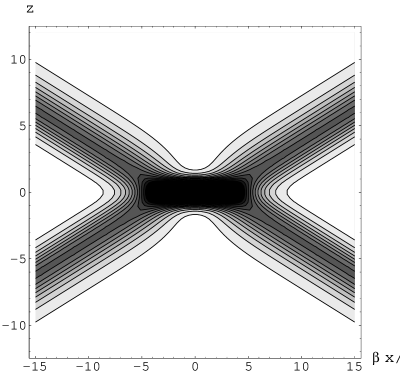
Figure 3: Contour plot of the energy density at the intersection of the domain walls as described within our Ansatz in terms of the scaling variable $\beta\,x/2$. Darker shading corresponds to larger energy density.

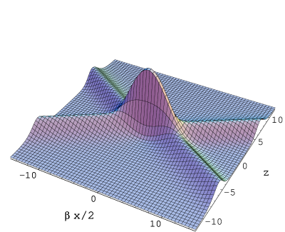
Figure 4: Three dimensional plot of the energy density at the intersection.

It is seen from the figures that the four crests of the energy density profile do not intersect at one point, rather there is a finite gap between the pairwise intersections of the energy crests for the ‘initial’ and the ‘final’ walls. In order to quantify this gap, we find from eqs.(16) and (7) the relation between $\sigma$ and $s$ as

$$\sigma=\int^{\infty}_{1/\cosh s}F(a)\,{\rm d}a$$ (17)

and then find numerically that at large $s$ this relation gives $\sigma=s+\delta$ with $\delta=1.7527\ldots$. Since at large $s$ the distance between the elementary walls is naturally identified as $2s$, one concludes that when the intersection of two walls is extrapolated from large distances it comes short of the actual center of the solution by the distance $2\delta/\beta$. The gap $\ell_{0}$ between the apparent pairwise collision vertices is then twice this distance. In this way we obtain the equation (1) with $\ell_{0}=4\,\delta=7.0108\ldots$ in the particular model with $\rho=4$.

In order to find the proper expression for the energy associated with the intersection, one can consider the problem of intersecting walls as a boundary value problem in a large box with the size $L$ in the $x$ direction (so that the boundaries are at $x=\pm L/2$), and at the boundaries the positions of the walls in the $z$ direction are specified as $s=\pm l/2$, where $s$ is the parameter in the expression (8) for the profile. (Clearly the sign of $h(z)$ at $x=+L/2$ should be chosen opposite to that at $x=-L/2$ in order to have an intersection configuration.) We also assume that the separation $l$ between the walls at the boundaries satisfies $l\ll L$ in order to correspond to $\beta\ll 1$. For free walls, with no energy associated with the intersection, the energy of such configuration would be determined by the total length of the walls in the box:

$$E_{0}=2\,\mu\,\sqrt{L^{2}+l^{2}}\approx 2\,\mu\,L+\mu\,L\,\left({l\over L}\right)^{2}~{}.$$ (18)

For the solution within our Ansatz, however, the energy is given by

$$E=2\,\mu\,L+\mu\,L\,{\beta^{2}\over 4}~{},$$ (19)

where $\beta/2$ is the slope in the solution $\sigma(x)=\beta\,x/2$. At $x=L/2$ one can use the asymptotic relation $\sigma=s+\delta$, and find from the boundary condition for $s$ the relation for $\beta$:

$${\beta\over 2}={l\over L}+{2\,\delta\over L}~{}.$$

Upon substituting this relation in eq.(19) one finds a finite difference between the expressions (19) and (18) for the energy: $\varepsilon=E-E_{0}$, given by our result in eq.(2).

If instead of the spatial coordinate $x$ one uses the time coordinate $t$, the discussed configuration describes a collision of two parallel walls (or two kinks in (1+1) dimensional theory). In this case the parameter of the intersection $\beta$ is identified as the relative velocity $v$ of the walls, and eq.(1) describes the time delay in the process of scattering of the walls, while the quantity $\varepsilon$ in eq.(2) gives the additional action with respect to the free motion of the walls, and thus is equal to the phase of the transmission amplitude in a quantum mechanical description of the scattering.

4 Discussion

The description of intersection of elementary domain walls is found here for small intersection angles and for a particular value of the parameter $\rho$, $\rho=4$, in a specific SUSY model. At present we can only speculate how our results are modified beyond these restrictions. Although the same Ansatz, as used here, can be applied in the limit of small $\beta$ at any value of $\rho$, one inevitably has to resort to numerical analysis because of lack of an explicit simple expressions for the profiles of the fields, except for the trivial case $\rho=1$. In particular, the existence of the gap at the intersection appears to be related to the existence of the special bifurcation solution[7] for parallel walls. Indeed a non-zero difference $\delta$ between $\sigma$ and $s$, arising from the integral in eq.(17), comes mostly from the integration over the values of $a$ past the bifurcation point, i.e. from $a=1$ to $a=\infty$. The bifurcation solution on the other hand exists in the considered model only for $\rho\geq 2$, and at $\rho=2$ the solution corresponds to $\chi(z)=0$, so that the bifurcation point is located at $x=0$ for such $\rho$. Our preliminary numerical study of the dependence of the size of the gap on $\rho$ indicates that indeed the gap appears to arise starting with $\rho=2$ and becomes larger with increasing $\rho$, whereas at $\rho<2$ we have found no apparent gap. This conjecture about such behavior is somewhat supported by the fact that at $\rho=1$ the elementary walls are not interacting and simply “go through” at the intersection with no gap whatsoever.

As to the dependence on the intersection parameter $\beta$, our Ansatz becomes inapplicable when $\beta$ is not small, and the behavior of the corresponding configurations is not known. Here we can only mention that the stability conditions[3] for the wall intersections allow a static quadruple intersection with any $\beta$ if $\rho>1$. Indeed in this case the energy of the non-BPS wall ($3\to 4$), $\mu_{34}=2\,\sqrt{\rho}\,\mu$ is larger than the sum of the energies of the elementary walls, and thus the quadruple intersection cannot split into triple ones, since the stability conditions for triple intersections can not be satisfied. On the contrary, at $\rho<1$ such splitting is possible with the critical value of $\beta$ defined as $\beta_{c}/(2\,\sqrt{1+(\beta_{c}/2)^{2}})=\sqrt{\rho}$.

BPS solitons are known to present effective low-energy degrees of freedom in some supersymmetric field theories. These effective (“dual”) theories exploit the fact that elementary solitons do not interact with each other at zero energies, both classically and quantum mechanically. This is just the case in the model considered, where the energy of parallel elementary domain walls does not depend on distance between them, and this degeneracy is not lifted by quantum corrections. We demonstrated here by an explicit calculation that some highly nontrivial interaction between BPS domain walls arises at nonzero momenta. If this observation holds for general case, to obtain dynamical information from dual models of that class appears to be an extremely complicated task.

5 Acknowledgements

One of us (SVT) acknowledges warm hospitality of the Theoretical Physics Institute at the University of Minnesota, where this work was done. The work of SVT is supported in part by the RFFI grant 96-02-17449a and in part by the U.S. Civilian Research and Development Foundation for Independent States of FSU (CRDF) Award No. RP1-187. The work of MBV is supported in part by DOE under the grant number DE-FG02-94ER40823.

References

- [1] T.D. Lee and G.C. Wick, Phys. Rev. D9 (1974) 2291.
- [2] Ya.B. Zeldovich, I.Yu. Kobzarev, and L.B. Okun, Zh.Eksp.Teor.Fiz. 67 (1974) 3 (Sov. Phys. JETP 40 (1974) 1).
- [3] M.B. Voloshin, Phys. Rev. D57 (1998) 1266.
- [4] G. Dvali and M. Shifman, Nucl. Phys. B504 (1997) 127.
- [5] G. Dvali and M. Shifman, Phys. Lett. B396 (1997) 64, Err.-ibid. B407 (1997) 452.
-
[6]
E. Bogomol’nyi, Sov. J. Nucl. Phys. 24 (1976) 449;
M.K. Prasad and C.H. Sommerfeld, Phys. Rev. Lett. 35 (1976) 760. - [7] M. Shifman, Phys. Rev. D57 (1998) 1258.
- [8] M.A. Shifman and M.B. Voloshin, Phys. Rev. D57 (1998) 2590.