US-FT-18/98

hep-th/9812105

Vassiliev Invariants in the Context of Chern-Simons Gauge Theory

J. M. F. Labastida and Esther Pérez

Departamento de Física de Partículas,
Universidade de Santiago de Compostela,
E-15706 Santiago de Compostela, Spain.

Abstract

We summarize the progress made during the last few years on the study of Vassiliev invariants from the point of view of perturbative Chern-Simons gauge theory. We argue that this approach is the most promising one to obtain a combinatorial universal formula for Vassiliev invariants. The combinatorial expressions for the two primitive Vassiliev invariants of order four, recently obtained in this context, are reviewed and rewritten in terms of Gauss diagrams.

Chern-Simons gauge theory has provided a very fruitful context to study knot and link invariants. The multiple approaches inherent to quantum field theory have been exploited to obtain different pictures for the resulting invariants. Non-perturbative methods [2, 3, 4, 5, 6, 7] have established the connection of Chern-Simons gauge theory with polynomial invariants as the Jones polynomial [8] and its generalizations [9, 10, 11]. Perturbative methods [12, 13, 14, 15, 16, 17, 18, 19] have provided representations of Vassiliev invariants [20]. The purpose of this lecture is to summarize the results obtained in recent years using the latter methods.

Though it became clear some years ago that the terms of the perturbative series expansion of Chern-Simons gauge theory were invariants of finite type [24, 21, 15, 22], we had to wait until last year to possess a field theory proof of this fact [23]. It was shown in [23], that, after constructing gauge invariant operators for singular knots, the terms of the perturbative series expansion of Chern-Simons gauge theory are invariants of finite type. The proof is gauge independent and therefore the property holds for any gauge-fixing. This result plus the fact that from a non-perturbative point of view Chern-Simons gauge theory leads to the Jones polynomial and its generalization constitutes a field theory proof of Birman and Lin theorem [22].

Theories possessing gauge invariance, as Chern-Simons gauge theory, can be studied performing different gauge fixings. Vacuum expectation values of gauge-invariant operators should be independent of the gauge fixing and they can therefore be computed in different gauges. Covariant gauges are simple to treat and its analysis in the case of perturbative Chern-Simons gauge theory has shown to lead to covariant formulae for Vassiliev invariants [12, 13, 15, 16, 17]. These formulae involve multidimensional space and path integrals which, in general, are rather involved to obtain the numerical value of Vassiliev invariants. Non-covariant gauges seem to lead to simpler formulae. However, the subtleties inherent in non-covariant gauges [26] plague their analysis with difficulties. The two non-covariant gauges more intensively studied are the light-cone gauge and the temporal gauge [27, 28, 29]. Both belong to the general category of axial gauges. In the light-cone gauge the resulting expressions for the Vassiliev invariants turn out to be the ones involving Kontsevich integrals [24]. This was proven in [19] and recently discussed in [25]. The resulting expressions, although simpler than the ones appearing in covariant gauges, are still too complicated to compute them explicitly. In the temporal gauge one obtains much simpler expressions. Actually, they do not involve integrations and are basically combinatorial [30]. Their explicit form up to order four has been presented in [30].

Combinatorial expressions for Vassiliev invariants have been seek since these invariants were formulated. To our knowledge, no other method have been able to lead to this type of expressions up to order four. An interesting combinatorial approach based on the use of Gauss diagrams was introduced in [31, 32]. One of the goals of this lecture is to show that the combinatorial expressions obtained in [30] can also be written in terms of Gauss diagrams. However, our main goal is to argue that Chern-Simons gauge theory is the most promising tool to build a combinatorial universal formula for Vassiliev invariants.

Non-covariant gauges are difficult to treat in any quantum field theory context [26]. Chern-Simons gauge theory is no exception to this. However, in this case, due to the exact knowledge on the theory at our disposal, it is known how the results obtained in a non-covariant gauge have to be modified to find agreement with their covariant counterpart. In computing vacuum expectation values of Wilson loops this turn out to be a simple multiplicative factor [19], as first pointed out by Kontsevich [24]. We will call this factor Kontsevich factor. A similar phenomena seems to be present in the temporal gauge. In this case it has been shown that the Kontsevich-like factor is not trivial and an explicit expression for it has been conjectured [30]. This conjecture has been proved up to order four. Understanding the origin of the Kontsevich factor one could gain some insight on some of the general problems inherent to non-covariant gauges.

We will begin reviewing the salient facts of the analysis of the perturbative series expansion of the vacuum expectation value of a Wilson loop in the temporal gauge carried out in [30]. Given a knot $K$ and one of its regular knot projections, ${\cal K}$, on the $x_{1},x_{2}$-plane which is a Morse knot in the $x_{1}$ and $x_{2}$ directions, one possesses a perturbative series expansion for the vacuum expectation value of the corresponding Wilson loop:

$$\langle W({K},G)\rangle=\langle W({{\cal K}},G)\rangle_{{\rm temp}}\times\langle W(U,G)\rangle^{b({\cal K})},$$ (1)

being,

$${1\over d}\langle W({K},G)\rangle=1+\sum_{i=1}^{\infty}v_{i}(K)x^{i},$$ (2)

and,

$${1\over d}\langle W({{\cal K}},G)\rangle_{{\rm temp}}=1+\sum_{i=1}^{\infty}\hat{v}_{i}({\cal K})x^{i}.$$ (3)

In these expressions $x$ denotes the inverse of the Chern-Simons coupling constant, $x=2\pi i/k$, $G$ the gauge group, and $d$ the dimension of the representation carried by the Wilson loop. The function $b({\cal K})$ is the exponent of the Kontsevich factor, which has been conjectured to be [30],

$$b({\cal K})={1\over 12}(n_{x_{1}}+n_{x_{2}}),$$ (4)

where $n_{x_{1}}$ and $n_{x_{2}}$ are the critical points of the regular projection ${\cal K}$ in both, the $x_{1}$ and the $x_{2}$ directions. In (1) $U$ denotes the unknot and $\langle W({{\cal K}},G)\rangle_{{\rm temp}}$ is the vacuum expectation of the Wilson line corresponding to the regular projection ${\cal K}$ as computed perturbatively in the temporal gauge with the standard Feynman rules of the theory. Notice that though each of the factors on the right hand side of (1) depends on the regular projection chosen, the left hand side does not. While the coefficients $v_{i}(K)$ of the series (2) are Vassiliev invariants the coefficients $\hat{v}_{i}(K)$ of (3) are not. The latter depend on the regular projection chosen.

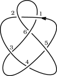
Figure 1: Example of a knot projection.

An explicit combinatorial form (no integrals left) of the coefficients $\hat{v}_{i}(K)$ in (3) would lead to a universal combinatorial formula for Vassiliev invariants. Unfortunately, this has not been obtained yet at all orders. Only part of the contributions entering $\hat{v}_{i}(K)$ have been explicitly written at all orders. These are the kernels introduced in [30]. The kernels are quantities which depend on the knot projection chosen and therefore are not knot invariants. However, at a given order $i$ a kernel differs from an invariant of type $i$ by terms that vanish in signed sums of order $i$. The kernel contains the part of a Vassiliev which is the last in becoming zero when performing signed sums, in other words, a kernel vanishes in signed sums of order $i+1$ but does not in signed sums of order $i$. In some sense the kernel represents the most fundamental part of a Vassiliev invariant, i.e., the part that survives a maximum number of signed sums. Kernels plus the structure of the perturbative series expansion seem to contain enough information to reconstruct the full Vassiliev invariants. This was shown in [30] up to order four. The results obtained there will be presented below and rewritten in a more compact form.

The expression for the kernels results after considering only the simplest part of the propagator of the gauge field in the temporal gauge. This part involves a double delta function and therefore all the integrals can be performed. The result is a combinatorial expression in terms of crossing signatures after distributing propagators among all the crossings. The general expression can be written in a universal form much in the spirit of the universal form of the Kontsevich integral [24]. Let us consider a knot $K$ with a regular knot projection ${\cal K}$ containing $n$ crossings. Let us choose a base point on ${\cal K}$ and let us label the $n$ crossings by $1,2,\dots,n$ as we pass for first time through each of them when traveling along ${\cal K}$ starting at the base point. The universal expression for the kernel associated to ${\cal K}$ has the form:

$${\cal N}({\cal K})=\sum_{k=0}^{\infty}\Bigg{(}\sum_{m=1}^{k}\sum_{p_{1},\dots,p_{m}=1\atop p_{1}+\cdots+p_{m}=k}^{k}\sum_{i_{1},\dots,i_{m}=1\atop i_{1}<\cdots<i_{m}}^{n}{\epsilon_{i_{1}}^{p_{1}}\cdots\epsilon_{i_{m}}^{p_{m}}\over(p_{1}!\cdots p_{m}!)^{2}}\sum_{\sigma_{1},\dots,\sigma_{m}\atop\sigma_{1}\in P_{1},\dots,\sigma_{m}\in P_{m}}{\cal T}(i_{1},\sigma_{1};\dots;i_{m},\sigma_{m})\Bigg{)}.$$ (5)

In this equation $P_{m}$ denotes the permutation group of $p_{m}$ elements. The factors in the innest sum, ${\cal T}(i_{1},\sigma_{1};\dots;i_{m},\sigma_{m})$, are group factors which are computed in the following way: given a set of crossings, $i_{1},\dots,i_{m}$, and a set of permutations, $\sigma_{1},\dots,\sigma_{m}$, with $\sigma_{1}\in P_{1},\dots,\sigma_{m}\in P_{m}$, the corresponding group factor ${\cal T}(i_{1},\sigma_{1};\dots;i_{m},\sigma_{m})$ is the result of taking a trace over the product of group generators which is obtained after assigning $p_{1},\dots,p_{m}$ group generators to the crossings $i_{1},\dots,i_{m}$ respectively, and placing each set of group generators in the order which results after traveling along the knot starting from the base point. The first time that one encounters a crossing $i_{j}$ a product of $p_{j}$ group generators is introduced; the second time the product is similar, but with the indices rearranged according to the permutation $\sigma_{j}\in P_{j}$.

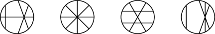
Figure 2: Chord diagrams corresponding to group factors.

In order to clarify the content of (5) we will work out an example. Let us consider the knot projection shown in fig. 1 and let us concentrate on some of the fourth order contributions, $k=4$. The knot projection under consideration has $n=5$ crossings. We will consider, for example, terms with $m=3$, and, $p_{1}=2$, $p_{2}=1$ and $p_{3}=1$. Since in this case the permutation groups $P_{2}$ and $P_{3}$ contain only the identity element, $1$, the form of the kernel is:

$${1\over(2!)^{2}}\sum_{i_{1},i_{2},i_{3}=1\atop i_{1}<i_{2}<i_{3}}^{6}\epsilon_{i_{1}}^{2}\epsilon_{i_{2}}\epsilon_{i_{3}}{\cal T}(i_{1},\sigma_{1};i_{2},1;i_{3},1),$$ (6)

where $\sigma_{1}\in P_{1}$, being $P_{1}$ the permutation group of 2 elements. Examples of the group factors entering this expression are:

$${\cal T}(1,\sigma_{1};2,1;3,1) = {\rm Tr}(T^{b_{1}}T^{b_{2}}T^{a_{1}}T^{a_{2}}T^{a_{1}}T^{\sigma_{1}(b_{1})}T^{\sigma_{1}(b_{2})}T^{a_{2}}),$$

$${\cal T}(1,\sigma_{1};3,1;5,1) = {\rm Tr}(T^{b_{1}}T^{b_{2}}T^{a_{1}}T^{a_{2}}T^{\sigma_{1}(b_{1})}T^{\sigma_{1}(b_{2})}T^{a_{1}}T^{a_{2}}),$$

$${\cal T}(2,\sigma_{1};3,1;6,1) = {\rm Tr}(T^{b_{1}}T^{b_{2}}T^{a_{1}}T^{a_{2}}T^{\sigma_{1}(b_{1})}T^{\sigma_{1}(b_{2})}T^{a_{2}}T^{a_{1}}),$$

$${\cal T}(3,\sigma_{1};4,1;6,1) = {\rm Tr}(T^{b_{1}}T^{b_{2}}T^{a_{1}}T^{a_{2}}T^{a_{2}}T^{\sigma_{1}(b_{1})}T^{\sigma_{1}(b_{2})}T^{a_{1}}),$$

where we have used the labels specified in fig. 1. Group factors can be represented by chord diagrams. For example if one chooses $\sigma_{1}=(12)$ the four chord diagrams corresponding to the group factors in (LABEL:masejem) are the ones pictured in fig. 2. The kernels are independent of the base point chosen for ${\cal K}$.

The universal formula (5) for the kernels can be written in a more useful way collecting all the coefficients multiplying a given group factor. The group factors can be labeled by chord diagrams. At order $k$ one has a term for each of the inequivalent chord diagrams with $k$ chords. Denoting chord diagrams by $D$, equation (5) can be written as:

$${\cal N}({\cal K})=\sum_{D}N_{D}({\cal K})D,$$ (8)

where the sum extends to all inequivalent chord diagrams. Our next task is to derive from (5) the general form of the kernels $N_{D}({\cal K})$. The concept of kernel can be extended to include singular knots by considering signed sums of (8), or, following [23], introducing vacuum expectation values of the operators for singular knots. If ${\cal K}^{j}$ denotes a regular projection of a knot $K^{j}$ with $j$ simple singular crossings or double points, the corresponding universal form for the kernel possesses an expansion similar to (8):

$${\cal N}({\cal K}^{j})=\sum_{D}N_{D}({\cal K}^{j})D.$$ (9)

The general results about singular knots proved in [23] lead to two important features for (9). On the one hand, finite type implies that $N_{D}({\cal K}^{j})=0$ for chord diagrams $D$ with more than $j$ chords. On the other hand, $N_{D}({\cal K}^{j})=2^{j}\delta_{D,D({\cal K}^{j})}$, where $D({\cal K}^{j})$ is the configuration corresponding to the singular knot projection ${\cal K}^{j}$. As observed above, kernels constitute the part of a Vassiliev invariant which survives a maximum number of signed sums.

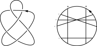
Figure 3: A regular knot projection and its corresponding Gauss diagram.

To compute $N_{D}({\cal K})$ we will introduce first the notion of the set of labeled chord subdiagrams of a given chord diagram. We will denote this set by $S_{D}$. This set is made out of a selected set of labeled chord diagrams that we now define.

A labeled chord diagram of order $p$ is a chord diagram with $p$ chords and a set of positive integers $k_{1},k_{2},\dots,k_{p}$, which will be called labels, such that each chord has one of these integers attached.

The set $S_{D}$ is made out of labeled chord diagrams which satisfy two conditions. These conditions are fixed by the form of the series entering the kernels (5). We will call the elements of $S_{D}$ labeled chord subdiagrams of the chord diagram $D$. They are defined as follows.

A labeled chord subdiagram of a chord diagram $D$ with $k$ chords is a labeled chord diagram of order $p$ with labels $k_{1},k_{2},\dots,k_{p}$, $p\leq k$, such that the following two conditions are satisfied:

a) $k_{1}+k_{2}+\cdots+k_{p}=k$;

b) there exist elements $\sigma_{1}\in P_{k_{1}},\sigma_{2}\in P_{k_{2}},\dots,\sigma_{p}\in P_{k_{p}}$ of the permutation groups $P_{k_{1}},P_{k_{2}},\dots,P_{k_{p}}$ such that, after replacing the $j$-th chord diagram by $k_{j}$ chords arranged according to the permutation $\sigma_{j}$, for $j=1,\dots,p$, the resulting chord diagram is homeomorphic to $D$. The number of ways that permutations $\sigma_{1}\in P_{k_{1}},\sigma_{2}\in P_{k_{2}},\dots,\sigma_{p}\in P_{k_{p}}$ can be chosen is called the multiplicity of the labeled chord subdiagram. We will denote the multiplicity of a given labeled chord subdiagram, $s\in S_{D}$, by $m_{D}(s)$.

The chord diagram $D$ itself can be regarded as a labeled chord subdiagram such that its labels, or positive integers attached to its chords, are 1. It has multiplicity 1. All the elements of $S_{D}$ except $D$ have a number of chords smaller than the number of chords of $D$. Not all labeled chord diagrams are subdiagrams of $D$. However, given a labeled chord diagram with labels $k_{1},k_{2},\dots,k_{p}$ there can be different sets of permutations leading to $D$. The number of these different sets is the multiplicity introduced above. The elements of the sets $S_{D}$ for all chord diagrams $D$ up to order four which do not have disconnected subdiagrams are the following:

$$\longrightarrow \hskip 8.5359pt\mbox{\leavevmode \hskip 15.0pt}\hbox{\hskip-11.38092pt},\mbox{\leavevmode \hskip 15.0pt} \longrightarrow \hskip 8.5359pt\mbox{\leavevmode \hskip 15.0pt}\hbox{\hskip-11.38092pt},\mbox{\leavevmode \hskip 15.0pt}\hbox{\hskip-11.38092pt},2\mbox{\leavevmode \hskip 15.0pt} \longrightarrow \hskip 8.5359pt\mbox{\leavevmode \hskip 15.0pt}\hbox{\hskip-11.38092pt},\mbox{\leavevmode \hskip 15.0pt}\hbox{\hskip-11.38092pt},\mbox{\leavevmode \hskip 15.0pt} \longrightarrow \hskip 8.5359pt\mbox{\leavevmode \hskip 15.0pt}\hbox{\hskip-11.38092pt},\mbox{\leavevmode \hskip 15.0pt}\hbox{\hskip-11.38092pt},\mbox{\leavevmode \hskip 15.0pt}\hbox{\hskip-11.38092pt},2\mbox{\leavevmode \hskip 15.0pt} \longrightarrow \hskip 8.5359pt\mbox{\leavevmode \hskip 15.0pt}\hbox{\hskip-11.38092pt},2\mbox{\leavevmode \hskip 15.0pt} \longrightarrow \hskip 8.5359pt\mbox{\leavevmode \hskip 15.0pt}\hbox{\hskip-11.38092pt},\mbox{\leavevmode \hskip 15.0pt}\hbox{\hskip-11.38092pt},2\mbox{\leavevmode \hskip 15.0pt}\hbox{\hskip-11.38092pt},4\mbox{\leavevmode \hskip 15.0pt} \longrightarrow \hskip 8.5359pt\mbox{\leavevmode \hskip 15.0pt}\hbox{\hskip-11.38092pt},\mbox{\leavevmode \hskip 15.0pt}\hbox{\hskip-11.38092pt},2\mbox{\leavevmode \hskip 15.0pt}\hbox{\hskip-11.38092pt},\mbox{\leavevmode \hskip 15.0pt} \longrightarrow \hskip 8.5359pt\mbox{\leavevmode \hskip 15.0pt}\hbox{\hskip-11.38092pt},\mbox{\leavevmode \hskip 15.0pt}\hbox{\hskip-11.38092pt},\mbox{\leavevmode \hskip 15.0pt}\hbox{\hskip-11.38092pt},2\mbox{\leavevmode \hskip 15.0pt}\hbox{\hskip-11.38092pt},2\mbox{\leavevmode \hskip 15.0pt}\hbox{\hskip-11.38092pt},3\mbox{\leavevmode \hskip 15.0pt} \longrightarrow \hskip 8.5359pt\mbox{\leavevmode \hskip 15.0pt}\hbox{\hskip-11.38092pt},\mbox{\leavevmode \hskip 15.0pt}\hbox{\hskip-11.38092pt},\mbox{\leavevmode \hskip 15.0pt}\hbox{\hskip-11.38092pt},\mbox{\leavevmode \hskip 15.0pt}\hbox{\hskip-11.38092pt},\mbox{\leavevmode \hskip 15.0pt}$$

The numbers accompanying each labeled chord subdiagram denote their multiplicity. When no number is attached to a chord of a labeled chord diagram it should be understood that the corresponding label is 1.

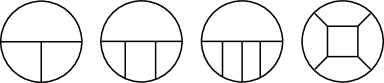
Figure 4: Basis of primitive Vassiliev invariant up to order four.

In order to write our final expression for the kernels we need to recall the notion of Gauss diagram. Given a regular projection ${\cal K}$ of a knot $K$ we can associate to it its Gauss diagram $G({\cal K})$. The regular projection ${\cal K}$ can be regarded as a generic immersion of a circle into the plane enhanced by information on the crossings. The Gauss diagram $G({\cal K})$ consists of a circle together with the preimages of each crossing of the immersion connected by a chord. Each chord is equipped with the sign of the signature of the corresponding crossing. An example of Gauss diagram has been pictured in fig. 3. Gauss diagrams are useful because they allow to keep track of the sums involving the crossings which enter in (5) in a very simple form. Let us consider a chord diagram $D$ and one of its labeled chord subdiagrams $s\in S_{D}$. Let us assume that $s$ has $p$ chords and labels $k_{1},k_{2},\cdots,k_{p}$. We define the product,

$$\langle s,G({\cal K})\rangle,$$ (11)

as the sum over all the embeddings of $s$ into $G({\cal K})$, each one weighted by a factor,

$${\epsilon_{1}^{k_{1}}\epsilon_{2}^{k_{2}}\cdots\epsilon_{p}^{k_{p}}\over(k_{1}!k_{2}!\cdots k_{p}!)^{2}},$$ (12)

where $\epsilon_{1},\epsilon_{2},\dots,\epsilon_{p}$ are the signatures of the chords of $G({\cal K})$ involved in the embedding. Using (11) the kernels $N_{D}({\cal K})$ entering (8) can be written as,

$$N_{D}({\cal K})=\sum_{s\in S_{D}}m_{D}(s)\langle s,G({\cal K})\rangle,$$ (13)

where $m_{D}(s)$ denotes the multiplicity of the labeled subdiagram $s\in S_{D}$ relative to the chord diagram $D$.

The product (11) possesses important properties. First, it is independent of the base point chosen for the regular projection ${\cal K}$ and, correspondingly, for the Gauss diagram $G({\cal K})$. Second, it is of finite type. This means that if $s$ has $j$ chords, the result of computing a signed sum of order higher than $j$ is zero. Recall that signed sums of order $k$ are used to define quantities associated to singular knot projections with $k$ double points, as the ones entering (8). A signed sum of order $k$ contains $2^{k}$ terms which correspond to the possible ways of resolving $k$ double points into overcrossings and undercrossings. Each one has a sign which corresponds to the product of the signatures of the crossings involved in the $k$ double points. If $s$ is a labeled chord diagram with $j$ chords and all its labels take value one, the order-$j$ signed sum is $2^{j}$ if the configuration of the singular projection with $j$ double points associated to such a sum corresponds to the chord diagram $s$; otherwise its value is zero. This fact leads to the result mentioned above stating that:

$$N_{D}({\cal K}^{j})=2^{j}\delta_{D,D({\cal K}^{j})},$$ (14)

where $D({\cal K}^{j})$ is the configuration corresponding to the singular knot projection associated to the signed sum. Of course, the product (11) vanishes if the number of chords of $s$ is bigger than the number of chords of the Gauss diagram $G({\cal K})$.

The products (11) can be regarded as quantities of finite type associated to Gauss diagrams $G$ whether or not these correspond to a regular projection of a knot. Gauss diagrams can be studied as abstract objects characterized by chord diagrams with signs assigned to their chords. It is clear that in such a general context the quantities $\langle s,G\rangle$, as defined in (11), are of finite type. In other words, if $s$ has $j$ chords and $G$ is an abstract Gauss diagram, the product $\langle s,G\rangle$ vanishes under signed sums of order higher than $j$. This observation leads to conjecture that the product (11) might play an interesting role in the theory of virtual knots [34, 35].

The terms $\langle s,G({\cal K})\rangle$ entering (13) are related to the quantities $\chi({\cal K})$ defined in [30]. It is straightforward to obtain the following relations:

$$\langle\mbox{\leavevmode \hskip 15.0pt}\hbox{\hskip-11.38092pt},G({\cal K})\rangle = {1\over(j!)^{2}}\chi_{1}({\cal K}),\hbox{\hskip 8.5359pt}j\hbox{\hskip 5.69046pt}\hbox{\rm odd,} \vbox{\vskip 25.6073pt}\langle\mbox{\leavevmode \hskip 15.0pt}\hbox{\hskip-11.38092pt},G({\cal K})\rangle = \chi_{2}^{A}({\cal K}), \vbox{\vskip 25.6073pt}\langle\mbox{\leavevmode \hskip 15.0pt}\hbox{\hskip-11.38092pt},G({\cal K})\rangle = {1\over 16}\chi_{2}^{C}({\cal K}), \vbox{\vskip 25.6073pt}\langle\mbox{\leavevmode \hskip 15.0pt}\hbox{\hskip-11.38092pt},G({\cal K})\rangle = \chi_{3}^{B}({\cal K}), \vbox{\vskip 25.6073pt}\langle\mbox{\leavevmode \hskip 15.0pt}\hbox{\hskip-11.38092pt},G({\cal K})\rangle = {1\over 4}\chi_{3}^{D}({\cal K}), \vbox{\vskip 25.6073pt}\langle\mbox{\leavevmode \hskip 15.0pt}\hbox{\hskip-11.38092pt},G({\cal K})\rangle = \chi_{4}^{A}({\cal K}), \vbox{\vskip 25.6073pt}\langle\mbox{\leavevmode \hskip 15.0pt}\hbox{\hskip-11.38092pt},G({\cal K})\rangle = \chi_{4}^{C}({\cal K}), \vbox{\vskip 25.6073pt}\langle\mbox{\leavevmode \hskip 15.0pt}\hbox{\hskip-11.38092pt},G({\cal K})\rangle = \chi_{4}^{E}({\cal K}),\vbox{\vskip 25.6073pt} \langle\mbox{\leavevmode \hskip 15.0pt}\hbox{\hskip-11.38092pt},G({\cal K})\rangle = {1\over(j!)^{2}}n({\cal K}),\hbox{\hskip 8.5359pt}j\hbox{\hskip 5.69046pt}\hbox{\rm even,} \vbox{\vskip 25.6073pt}\langle\mbox{\leavevmode \hskip 15.0pt}\hbox{\hskip-11.38092pt},G({\cal K})\rangle = {1\over 4}\chi_{2}^{B}({\cal K}), \vbox{\vskip 25.6073pt}\langle\mbox{\leavevmode \hskip 15.0pt}\hbox{\hskip-11.38092pt},G({\cal K})\rangle = \chi_{3}^{A}({\cal K}), \vbox{\vskip 25.6073pt}\langle\mbox{\leavevmode \hskip 15.0pt}\hbox{\hskip-11.38092pt},G({\cal K})\rangle = {1\over 4}\chi_{3}^{C}({\cal K}), \vbox{\vskip 25.6073pt}\langle\mbox{\leavevmode \hskip 15.0pt}\hbox{\hskip-11.38092pt},G({\cal K})\rangle = {1\over 4}\chi_{3}^{E}({\cal K}), \vbox{\vskip 25.6073pt}\langle\mbox{\leavevmode \hskip 15.0pt}\hbox{\hskip-11.38092pt},G({\cal K})\rangle = \chi_{4}^{B}({\cal K}), \vbox{\vskip 25.6073pt}\langle\mbox{\leavevmode \hskip 15.0pt}\hbox{\hskip-11.38092pt},G({\cal K})\rangle = \chi_{4}^{D}({\cal K}), \vbox{\vskip 25.6073pt}\langle\mbox{\leavevmode \hskip 15.0pt}\hbox{\hskip-11.38092pt},G({\cal K})\rangle = \chi_{4}^{F}({\cal K}).$$

Notice that in the second relation $n({\cal K})$ denotes the number of crossings of the regular projection ${\cal K}$. The rest of the quantities on the right hand side of (1) were defined in [30].

In [30] we were able to express all the Vassiliev invariants up to order four in terms of these quantities and the crossing signatures. The strategy was to start with the kernels (13) and exploit the properties of the perturbative series expansion of Chern-Simons gauge theory. A special role in the construction was played by the factorization theorem proved in [33]. At orders two and three there is only one primitive Vassiliev invariant. We will make the same choice of basis as in [30]. The diagrams associated to them are the first two in fig. 4. The two primitive Vassiliev invariants turn out to be, at second order,

$$\alpha_{21}(K)=\alpha_{21}(U)+\langle\mbox{\leavevmode \hskip 15.0pt}\hbox{\hskip-11.38092pt},\bar{G}({\cal K})\rangle,$$ (16)

while, at third order,

$$\alpha_{31}(K)=\langle\mbox{\leavevmode \hskip 15.0pt}\hbox{\hskip-11.38092pt}+\mbox{\leavevmode \hskip 15.0pt}\hbox{\hskip-11.38092pt}+2\mbox{\leavevmode \hskip 15.0pt}\hbox{\hskip-11.38092pt},G({\cal K})\rangle-\sum_{i=1}^{n}\,\epsilon_{i}({\cal K})\Big{[}\langle\mbox{\leavevmode \hskip 15.0pt}\hbox{\hskip-11.38092pt},G(\alpha({\cal K}))\rangle\Big{]}_{i}.$$ (17)

Several comments are in order to explain the quantities entering these expressions. In (16) $\alpha_{21}(U)$ stands for the value of the invariant $\alpha_{21}$ for the unknot. In the first equation the bar denotes that the product has to be taken on $G({\cal K})$ and then substract its value for the ascending diagram. In general a bar over a quantity $L({\cal K})$ indicates that the same quantity for the ascending diagram has to be subtracted, i.e.:

$$\bar{L}({\cal K})=L({\cal K})-L(\alpha({\cal K}))$$ (18)

where $\alpha({\cal K})$ denotes the standard ascending diagram of ${\cal K}$. The ascending diagram of a knot projection is defined as the diagram obtained by switching, when traveling along the knot from a base point, all the undercrossings to overcrossings. In (17) the sum is over all crossings $i$, $i=1,\dots,n$, and $\epsilon_{i}({\cal K})$ denotes the corresponding signature. The square brackets $[$ $]_{i}$ enclosing a quantity $L({\cal K})$ denote:

$$\Big{[}L({\cal K})\Big{]}_{i}=L({\cal K})-L({\cal K}_{i_{+}})-L({\cal K}_{i_{-}}),$$ (19)

where the regular projection diagrams ${\cal K}_{i_{+}}$ and ${\cal K}_{i_{-}}$ are the ones which result after the splitting of ${\cal K}$ at the crossing point $i$ as shown in the first row of fig. 5. It is clear from the list (1) that these two invariants can be written in terms of the products (11) and the crossing signatures.

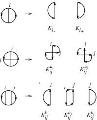
Figure 5: Splitting a knot into other knots.

Combinatorial expressions for the two primitive invariants at order four have been presented in [30]. Their construction is based on the use of the kernels (13) and the properties of the perturbative series expansion. As in the case of previous orders, these invariants are expressed in terms of the products (11) and the crossing signatures. Their form is more complicated than the ones at lower orders. They turn out to be:

$${\hskip-14.22636pt}\alpha_{42}(K)=\alpha_{42}(U)+\langle 7\mbox{\leavevmode \hskip 15.0pt}\hbox{\hskip-11.38092pt}+5\mbox{\leavevmode \hskip 15.0pt}\hbox{\hskip-11.38092pt}+4\mbox{\leavevmode \hskip 15.0pt}\hbox{\hskip-11.38092pt}+2\mbox{\leavevmode \hskip 15.0pt}\hbox{\hskip-11.38092pt}+\mbox{\leavevmode \hskip 15.0pt}\hbox{\hskip-11.38092pt}+\mbox{\leavevmode \hskip 15.0pt}\hbox{\hskip-11.38092pt}$$

$$\hbox{\hskip 175.83781pt}+8\mbox{\leavevmode \hskip 15.0pt}\hbox{\hskip-11.38092pt}+2\mbox{\leavevmode \hskip 15.0pt}\hbox{\hskip-11.38092pt}+8\mbox{\leavevmode \hskip 15.0pt}\hbox{\hskip-11.38092pt}+{1\over 6}\mbox{\leavevmode \hskip 15.0pt}\hbox{\hskip-11.38092pt},\bar{G}({\cal K})\rangle$$

$$+\sum_{i,j\in{\cal C}_{a}\atop i>j}\bar{\epsilon}_{ij}({\cal K})\Bigg{(}\Big{[}\langle\mbox{\leavevmode \hskip 15.0pt}\hbox{\hskip-11.38092pt},G(\alpha({\cal K}))\rangle\Big{]}_{ij}^{a}-2\Big{[}\langle\mbox{\leavevmode \hskip 15.0pt}\hbox{\hskip-11.38092pt},G(\alpha({\cal K}))\rangle\Big{]}_{i}-2\Big{[}\langle\mbox{\leavevmode \hskip 15.0pt}\hbox{\hskip-11.38092pt},G(\alpha({\cal K}))\rangle\Big{]}_{j}\Bigg{)}$$

$$+\sum_{i,j\in{\cal C}_{b}\atop i>j}\bar{\epsilon}_{ij}({\cal K})\Bigg{(}\Big{[}\langle\mbox{\leavevmode \hskip 15.0pt}\hbox{\hskip-11.38092pt},G(\alpha({\cal K}))\rangle\Big{]}_{ij}^{b}-\Big{[}\langle\mbox{\leavevmode \hskip 15.0pt}\hbox{\hskip-11.38092pt},G(\alpha({\cal K}))\rangle\Big{]}_{i}-\Big{[}\langle\mbox{\leavevmode \hskip 15.0pt}\hbox{\hskip-11.38092pt},G(\alpha({\cal K}))\rangle\Big{]}_{j}\Bigg{)},$$

(20)

and,

$${\hskip-19.91684pt}\alpha_{43}(K)=\alpha_{43}(U)+\langle\mbox{\leavevmode \hskip 15.0pt}\hbox{\hskip-11.38092pt}+\mbox{\leavevmode \hskip 15.0pt}\hbox{\hskip-11.38092pt}+\mbox{\leavevmode \hskip 15.0pt}\hbox{\hskip-11.38092pt}+2\mbox{\leavevmode \hskip 15.0pt}\hbox{\hskip-11.38092pt}-{1\over 6}\mbox{\leavevmode \hskip 15.0pt}\hbox{\hskip-11.38092pt},\bar{G}({\cal K})\rangle$$

$$+\sum_{i,j\in{\cal C}_{a}\atop i>j}\bar{\epsilon}_{ij}({\cal K})\Bigg{(}\Big{[}\langle\mbox{\leavevmode \hskip 15.0pt}\hbox{\hskip-11.38092pt},G(\alpha({\cal K}))\rangle\Big{]}_{ij}^{a}-\Big{[}\langle\mbox{\leavevmode \hskip 15.0pt}\hbox{\hskip-11.38092pt},G(\alpha({\cal K}))\rangle\Big{]}_{i}-\Big{[}\langle\mbox{\leavevmode \hskip 15.0pt}\hbox{\hskip-11.38092pt},G(\alpha({\cal K}))\rangle\Big{]}_{j}\Bigg{)}.$$

(21)

In these expressions the explicit dependence on the signatures appears in the quantities $\bar{\epsilon}_{ij}({\cal K})$ which are:

$$\bar{\epsilon}_{ij}({\cal K})=\epsilon_{ij}({\cal K})-\epsilon_{ij}(\alpha({\cal K}))=\epsilon_{i}({\cal K})\epsilon_{j}({\cal K})-\epsilon_{i}(\alpha({\cal K}))\epsilon_{j}(\alpha({\cal K})).$$ (22)

The sums in which these products are involved are over double splittings of the knot projection ${\cal K}$ at the crossings $i$ and $j$. There are two ways of carrying out these double splittings, depending on the configuration associated to the crossings $i$ and $j$. These are shown in the second and third rows of fig. 5. In the first one the regular projection ${\cal K}$ is split into two while in the second one it is split into three. Splittings of the first type build the set ${\cal C}_{a}$. The ones of the second type build ${\cal C}_{b}$. While only the first one is involved in the invariant $\alpha_{43}$, both appear in $\alpha_{42}$. The new quantities entering the sums are:

$$\Big{[}L({\cal K})\Big{]}_{ij}^{a} = L({\cal K})-L({\cal K}_{ij}^{a_{1}})-L({\cal K}_{ij}^{a_{2}}),$$

$$\Big{[}L({\cal K})\Big{]}_{ij}^{b} = L({\cal K})-L({\cal K}_{ij}^{b_{1}})-L({\cal K}_{ij}^{b_{2}})-L({\cal K}_{ij}^{b_{3}}),$$ (23)

where ${\cal K}_{ij}^{a_{1}},{\cal K}_{ij}^{a_{2}},{\cal K}_{ij}^{b_{1}},{\cal K}_{ij}^{b_{2}}$ and ${\cal K}_{ij}^{b_{3}}$ are the knot projections which originate after a double splitting of ${\cal K}$, as denoted in fig. 5. As in previous orders, in the expressions (20) and (21), the quantities $\alpha_{42}(U)$ and $\alpha_{43}(U)$ correspond to the value of these invariants for the unknot. It has been proved in [30] that the combinatorial expressions for $\alpha_{42}(K)$ and $\alpha_{43}(K)$ in (20) and (21) are invariant under Reidemeister moves.

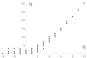
Figure 6: Plot of the absolute value of the third-order Vassiliev invariant $\nu_{3}$ versus the one of order two, $\nu_{2}$, for all prime knots up to nine crossings.

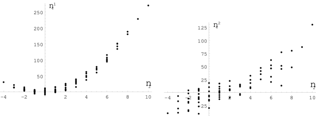
Figure 7: Plots of the two fourth-order Vassiliev invariants $\nu_{4}^{1}$ and $\nu_{4}^{2}$ versus the second order one $\nu_{2}$, for all prime knots up to nine crossings.

Vassiliev invariants constitute vector spaces and their normalization can be chosen in such a way that they are integer-valued. Once their value for the unknot has been subtracted off they can be presented in many basis in which they are integers. We will chose here a particular basis in which the numerical values for the invariants up to order four are rather simple:

$$\nu_{2}(K) = {1\over 4}\tilde{\alpha}_{21}(K),$$

$$\nu_{3}(K) = {1\over 8}\tilde{\alpha}_{31}(K),$$

$$\nu_{4}^{1}(K) = {1\over 8}(\tilde{\alpha}_{42}(K)+\tilde{\alpha}_{43}(K)),$$

$$\nu_{4}^{2}(K) = {1\over 4}(\tilde{\alpha}_{42}(K)-5\tilde{\alpha}_{43}(K)),$$

where the tilde indicates that the value for the unknot has been subtracted, i.e., $\tilde{\alpha}_{ij}(K)=\alpha_{ij}(K)-\alpha_{ij}(U)$. In Tables 1 and 2 we have collected the value of the Vassiliev invariants (LABEL:basica) for all prime knots up to nine crossings. Notice that we could have chosen a basis where all the values for the trefoil knot are 1 just redefining $\nu_{4}^{1}(K)$ into $\nu_{4}^{1}(K)-2\nu_{4}^{2}(K)$. We have no done so because $\nu_{4}^{1}(K)$, as defined in (LABEL:basica), has a simple shape when plotted versus $\nu_{2}(K)$. Actually, the resulting shape has features similar to the shape which results after plotting $\nu_{3}(K)$ versus $\nu_{2}(K)$. In fig. 7 we present $\nu_{4}^{1}(K)$ and $\nu_{4}^{2}(K)$ versus $\nu_{2}(K)$. These should be compared to the plot of the absolute value of $\nu_{3}(K)$ versus $\nu_{2}(K)$ depicted in fig. 6. The similar behavior observed for $|\nu_{3}(K)|$ and $\nu_{4}^{2}(K)$ is expected from their general form for torus knots. As it was shown in [16] and [36], for a torus knot characterized by two coprime integers $p$ and $q$ these invariants are the following polynomials in $p$ and $q$:

$$\nu_{2}(p,q) = {1\over 24}(p^{2}-1)(q^{2}-1)$$

$$\nu_{3}(p,q) = {1\over 144}(p^{2}-1)(q^{2}-1)pq$$

$$\nu_{4}^{1}(p,q) = {1\over 288}(p^{2}-1)(q^{2}-1)p^{2}q^{2}$$ (25)

$$\nu_{4}^{2}(p,q) = {1\over 720}(p^{2}-1)(q^{2}-1)(2p^{2}q^{2}-3p^{2}-3q^{2}-3)$$

The explicit expression of Vassiliev invariants as polynomials in $p$ and $q$ is known up to order six [16]. Of course, up to order four their value agree with the ones computed explicitly from equations (20) and (21), as it can be checked explicitly from the tables collected below. The only torus knots up to nine crossings are $3_{1}$, $5_{1}$, $7_{1}$, $8_{19}$ and $9_{1}$, whose associated coprime integers are (3,2), (5,2), (7,2), (4,3) and (9,2), respectively.

It would be desirable to write the invariants in such a way that signatures and split sums do not appear. Even better would be to possess expressions where terms involving ascending diagrams are not present. It is not known if this is possible even for the few orders in which combinatorial expressions for the invariants exist. There are indications however that in order to achieve such a goal arrow diagrams as the ones used in [31] have to be introduced. The effect of the introduction of these diagrams is to reduce the amount of embeddings entering the product (11) to a selected set. Both, the expressions and the amount of calculation could notably simplify if this is possible. This issue is under investigation.

Our approach opens a variety of investigations. First of all a generalization of the reconstruction procedure from the kernels (5) presented in [30] up to order four should be constructed. This could lead to a universal combinatorial formula for Vassiliev invariants. The approach is also well suited to obtain combinatorial expressions for Vassiliev invariants for links, a field which has not been much explored up to now. Another context in which our approach could be also very powerfull is in the study of vacuum expectation values of graphs, quantities that plays an important role in recent developments in the canonical approach to quantum gravity [37]. Vassiliev invariants for graphas constitute a rather unexplored field which could lead to new sets of important invariants.

Acknowledgements

We would like to thank L. Alvarez-Gaumé and M. Alvarez for helpful discussions on Vassiliev invariants and on gauge fixing. We also thank Simon Willerton for bringing Gauss diagrams to our attention and for sending us a copy of his Ph. D. thesis. J.M.F.L. would like to thank the organizers of the workshop on “New Developments in Algebraic Topology” for their kind invitation and their hospitality. This work was supported in part by DGICYT under grant PB96-0960, and by the EU Commission under the TMR grant FMAX-CT96-0012.

Knot	$\nu_{2}$	$\nu_{3}$	$\nu_{4}^{1}$	$\nu_{4}^{2}$		Knot	$\nu_{2}$	$\nu_{3}$	$\nu_{4}^{1}$	$\nu_{4}^{2}$
$3_{1}$	1	1	3	1		$8_{5}$	$-$1	$-$3	1	$-41$
$4_{1}$	$-$1	0	2	-3		$8_{6}$	$-$2	$-$3	7	-36
$5_{1}$	3	5	25	11		$8_{7}$	2	$-$2	4	22
$5_{2}$	2	3	13	4		$8_{8}$	2	$-$1	5	12
$6_{1}$	$-$2	$-$1	7	$-12$		$8_{9}$	$-$2	0	14	-34
$6_{2}$	$-$1	$-$1	3	$-13$		$8_{10}$	3	$-$3	15	15
$6_{3}$	1	0	0	7		$8_{11}$	$-$1	$-$2	2	-27
$7_{1}$	6	14	98	46		$8_{12}$	$-$3	0	14	$-17$
$7_{2}$	3	6	32	13		$8_{13}$	1	$-$1	$-1$	17
$7_{3}$	5	11	73	25		$8_{14}$	0	0	4	$-16$
$7_{4}$	4	8	50	8		$8_{15}$	4	7	37	18
$7_{5}$	4	8	46	24		$8_{16}$	1	$-$1	$-1$	17
$7_{6}$	1	2	8	-1		$8_{17}$	$-$1	0	6	$-19$
$7_{7}$	$-$1	1	$-$1	3		$8_{18}$	1	0	4	$-9$
$8_{1}$	$-3$	$-3$	13	$-31$		$8_{19}$	5	10	60	35
$8_{2}$	0	$-$1	3	30		$8_{20}$	2	2	8	6
$8_{3}$	$-4$	0	30	$-40$		$8_{21}$	0	$-$1	$-$1	$-14$
$8_{4}$	$-3$	1	21	-39

Table 1: Primitive Vassiliev invariants up to order four for all prime knots up to eight crossings.

Knot	$\nu_{2}$	$\nu_{3}$	$\nu_{4}^{1}$	$\nu_{4}^{2}$		Knot	$\nu_{2}$	$\nu_{3}$	$\nu_{4}^{1}$	$\nu_{4}^{2}$
$9_{1}$	10	30	270	130		$9_{26}$	0	1	$-$5	2
$9_{2}$	4	10	62	32		$9_{27}$	0	1	3	$-6$
$9_{3}$	9	26	228	87		$9_{28}$	1	0	$-$2	3
$9_{4}$	7	19	151	51		$9_{29}$	1	$-$2	2	11
$9_{5}$	6	15	115	20		$9_{30}$	$-$1	$-$1	5	$-9$
$9_{6}$	7	18	134	77		$9_{31}$	2	2	8	6
$9_{7}$	5	12	78	47		$9_{32}$	$-$1	2	$-$2	$-11$
$9_{8}$	0	2	8	-8		$9_{33}$	1	$-$1	3	1
$9_{9}$	8	22	180	80		$9_{34}$	$-$1	0	2	$-3$
$9_{10}$	8	22	188	48		$9_{35}$	7	18	150	13
$9_{11}$	4	$-$9	57	10		$9_{36}$	3	$-$7	39	15
$9_{12}$	1	3	15	1		$9_{37}$	$-$3	1	13	$-7$
$9_{13}$	7	18	142	45		$9_{38}$	6	14	98	46
$9_{14}$	$-$1	2	$-$6	5		$9_{39}$	2	$-$4	24	$-10$
$9_{15}$	2	$-$5	25	4		$9_{40}$	$-$1	$-$1	3	$-13$
$9_{16}$	6	14	94	62		$9_{41}$	0	1	$-$9	18
$9_{17}$	$-$2	0	6	$-2$		$9_{42}$	$-$2	0	10	$-18$
$9_{18}$	6	15	107	52		$9_{43}$	1	2	14	$-13$
$9_{19}$	$-$2	1	3	4		$9_{44}$	0	1	$-1$	10
$9_{20}$	2	4	20	6		$9_{45}$	2	$-$4	20	6
$9_{21}$	3	$-$6	36	$-3$		$9_{46}$	$-$2	$-$3	3	$-20$
$9_{22}$	$-$1	1	1	7		$9_{47}$	$-$1	$-$2	$-$6	5
$9_{23}$	5	11	69	41		$9_{48}$	3	$-$5	29	$-5$
$9_{24}$	1	2	6	$-5$		$9_{49}$	6	14	102	30
$9_{25}$	0	1	11	$-14$

Table 2: Primitive Vassiliev invariants up to order four for all prime knots with nine crossings.

References

- [1]
- [2] E. Witten, Commun. Math. Phys. 121 (1989) 351.
- [3] M. Bos and V.P. Nair, Phys. Lett. B223 (1989) 61 and Int. J. Mod. Phys. A5 (1990) 959; S. Elitzur, G. Moore, A. Schwimmer and N. Seiberg, Nucl. Phys. B326 (1989) 108.
- [4] J.M.F. Labastida and A.V. Ramallo, Phys. Lett. B227 (1989) 92 and B228 (1989) 214; J.M.F. Labastida, P.M. Llatas and A.V. Ramallo, Nucl. Phys. B348 (1991) 651; J.M.F. Labastida and M. Mariño, Int. J. Mod. Phys. A10 (1995) 1045; J.M.F. Labastida and E. Pérez, J. Math. Phys. 37 (1996) 2013.
- [5] J. Frohlich and C. King, Commun. Math. Phys. 126 (1989) 167.
- [6] S. Martin, Nucl. Phys. B338 (1990) 244.
- [7] R.K. Kaul and T.R. Govindarajan, Nucl. Phys. B380 (1992) 293 and B393 (1993) 392; P. Ramadevi, T.R. Govindarajan and R.K. Kaul, Nucl. Phys. B402 (1993) 548; Mod. Phys. Lett. A10 (1995) 1635; R.K. Kaul, Commun. Math. Phys. 162 (1994) 289; “Chern-Simons Theory, Knot Invariants, Vetex Models and Three-Manifold Invariants, hep-th/9804122.
- [8] V. F. R. Jones, Bull. AMS 12 (1985) 103; Ann. of Math. 126 (1987) 335.
- [9] P. Freyd, D. Yetter, J. Hoste, W.B.R. Lickorish, K. Millet and A. Ocneanu, Bull. AMS 12 (1985) 239.
- [10] L.H. Kauffman, Trans. Am. Math. Soc. 318 (1990) 417.
- [11] Y. Akutsu and M. Wadati, J. Phys. Soc. Jap. 56 (1987) 839 and 3039.
- [12] E. Guadagnini, M. Martellini and M. Mintchev, Phys. Lett. B227 (1989) 111 and B228 (1989) 489; Nucl. Phys. B330 (1990) 575.
- [13] D. Bar-Natan, “Perturbative aspects of Chern-Simons topological quantum field theory”, Ph.D. Thesis, Princeton University, 1991.
- [14] J.F.W.H. van de Wetering, Nucl. Phys. B379 (1992) 172.
- [15] M. Alvarez and J.M.F. Labastida, Nucl. Phys. B395 (1993) 198, hep-th/9110069, and B433 (1995) 555, hep-th/9407076; Erratum, ibid. B441 (1995) 403.
- [16] M. Alvarez and J.M.F. Labastida, Journal of Knot Theory and its Ramifications 5 (1996) 779; q-alg/9506009.
- [17] D. Altschuler and L. Friedel, Commun. Math. Phys. 187 (1997) 261 and 170 (1995) 41.
- [18] M. Alvarez, J.M.F. Labastida and E. Pérez, Nucl. Phys. B488 (1997) 677.
- [19] J.M.F. Labastida and E. Pérez, J. Math. Phys. 39 (1998) 5183; hep-th/9710176.
- [20] V. A. Vassiliev, “Cohomology of knot spaces”, Theory of singularities and its applications, Advances in Soviet Mathematics, vol. 1, Americam Math. Soc., Providence, RI, 1990, 23-69.
- [21] D. Bar-Natan, Topology 34 (1995) 423.
- [22] J.S. Birman and X.S. Lin, Invent. Math. 111 (1993) 225; J.S. Birman, Bull. AMS 28 (1993) 253.
- [23] J.M.F. Labastida and E. Pérez, Nucl. Phys. B527 (1998) 499, hep-th/9712139.
- [24] M. Kontsevich, Advances in Soviet Math. 16, Part 2 (1993) 137.
- [25] L. Kauffman, “Witten’s Integral and Kontsevich Integral”, preprint.
- [26] G. Leibbrandt, Rev. Mod. Phys. 59 (1987) 1067.
- [27] A.S. Cattaneo, P. Cotta-Ramusino, J. Frohlich and M. Martellini, J. Math. Phys. 36 (1995) 6137.
- [28] C. P. Martin, Phys. Lett. B241 (1990) 513; G. Giavarini, C.P. Martin and F. Ruiz Ruiz, Nucl. Phys. B381 (1992) 222.
- [29] G. Leibbrandt and C.P. Martin, Nucl. Phys. B377 (1992) 593 and B416 (1994) 351.
- [30] J.M.F. Labastida and E. Pérez, “Combinatorial Formulae for Vassiliev Invariants from Chern-Simons Gauge Theory”, CERN and Santiago de Compostela preprint, CERN-TH/98-193, US-FT-11/98; hep-th/9807155.
- [31] M. Goussarov, M. Polyak and O. Viro, Int. Math. Res. Notices 11 (1994) 445.
- [32] S. Willerton, “On the Vassiliev Invariants for Knots and Pure Braids”, Ph. D. Thesis, University of Edinburgh, 1997.
- [33] M. Alvarez and J.M.F. Labastida, Commun. Math. Phys. 189 (1997) 641, q-alg/9604010.
- [34] L. H. Kauffman, “Virtual Knot Theory”, preprint, 1998.
- [35] M. Goussarov, M. Polyak and O. Viro, “Finite Type Invariants of Classical and Virtual Knots”, preprint, 1998, math.GT/9810073.
- [36] S. Willerton, “On Universal Vassiliev Invariants, Cabling, and Torus Knots”, University of Melbourne preprint (1998).
- [37] R. Gambini, J. Griego and J. Pullin, Phys. Lett. B425 (1998) 41 and Nucl. Phys. B534 (1998) 675.