KANAZAWA/98-22

Non-Perturbative Renormalization Group
and Quantum Tunnelling

Ken-Ichi Aoki ,  Atsushi Horikoshi ,  Masaki Taniguchi
and   Haruhiko Terao

Institute for Theoretical Physics, Kanazawa University,

Kakuma-machi Kanazawa 920-1192, Japan

The non-perturbative renormalization group (NPRG) is applied to analysis of tunnelling in quantum mechanics. The vacuum energy and the energy gap of anharmonic oscillators are evaluated by solving the local potential approximated Wegner-Houghton equation (LPA W-H eqn.). We find that our results are very good in a strong coupling region, but not in a very weak coupling region, where the dilute gas instanton calculation works very well. So it seems that in analysis of quantum tunnelling, the dilute gas instanton and LPA W-H eqn. play complementary roles to each other. We also analyze the supersymmetric quantum mechanics and see if the dynamical supersymmetry (SUSY) breaking is described by NPRG method.

1 Introduction

The theoretical basis of NPRG was formulated by K.G.Wilson in 1970’s.[1] After that, several types of ‘exact’ renormalization group equations were derived and have been applied to various quantum systems. Although those equations are exact, we can not solve them without any approximation in practice. Therefore it is not trivial that such NPRG analysis can take account of the effects caused by non-perturbative dynamics even qualitatively.

Generally, there are two types of non-perturbative quantities. One corresponds to summation of all orders of the perturbative series, which might be related to the Borel resummation.[2] The other is the essential singularity with respect to coupling constant $\lambda$, which has a structure like $e^{-\frac{1}{\lambda}}$.[3] We are not able to expand this singular contribution around the origin of $\lambda$. This singularity is essential in case of quantum tunnelling. For example, in the symmetric double well system, there are degenerated two energy levels at each minima, which are mixed through tunnelling to generate an energy gap $\Delta E\sim e^{-\frac{1}{\lambda}}$. The exponential factor comes from the free energy of topological configurations, the instantons. Can NPRG evaluate these non-perturbative effects in a good manner? The main purpose of our work is to check this not only qualitatively but also quantitatively. We carry it out in quantum mechanical systems by comparing our results with the exact values given by numerical analysis of the Schrödinger equation, with the perturbative series, and with the instanton method. The instanton method is a unique analysis of quantum tunnelling leading to the exact essential singularity, which is, however, valid only in a very weak coupling region. It will turn out that the instanton method and LPA W-H eqn. are somehow complementary to each other.

Though quantum tunnelling is one of the most striking consequences of quantum theories, there has been no general-purpose tool to analyze it. So if NPRG treats non-perturbative dynamics well, it can be a powerful new tool for analysis of tunnelling and this work will be the first touch to attack more complex systems with quantum tunnelling by NPRG.

2 The NPRG study of quantum mechanics

As a primary study, we would like to restrict ourselves to treat the effective potential. We start with the LPA W-H eqn. for scalar theories, where we ignore the corrections to the derivative interactions,[4, 5]

$${\partial\hat{V}_{\rm eff}\over\partial\tau}=\left[D-d_{{\varphi}}\hat{\varphi}{\partial\over\partial\hat{\varphi}}\right]\hat{V}_{\rm eff}+{A_{D}\over 2}\log\left(1+{\partial^{2}\hat{V}_{\rm eff}\over\partial\hat{\varphi}\partial\hat{\varphi}}\right).$$ (1)

Each hatted($~{}\hat{}~{}$) variable represents a dimensionless quantity with a unit defined by the momentum cut off $\Lambda(\tau)=\rm e^{-\tau}\Lambda_{\rm 0}$, $D$ is the space-time dimension, $d_{\varphi}=\frac{D-2}{2}$ is the canonical dimension of scalar field $\varphi$, and $A_{D}=(2\pi)^{-D}\int d\Omega_{D}$. This is a partial differential equation of the dimensionless effective potential $\hat{V}_{\rm eff}$ with respect to $\hat{\varphi}$ and scale parameter $\tau$.

Furthermore, we expand $V_{\rm eff}$ as power series of $\varphi$,

$$V_{\rm eff}\left(\varphi;\tau\right) = \sum_{n=0}^{N}\frac{a_{n}(\tau)}{n!}\varphi^{n},$$ (2)

which is called the operator expansion. If the results converge as the order of truncation $N$ becomes large, we regard them as the solutions of LPA W-H eqn. The partial differential equation is reduced to a set of ordinary differential equations for dimensionless couplings $\{\hat{a}_{n}\}$,

$${d\hat{a}_{0}\over d\tau} = ~{}~{}~{}~{}~{}~{}~{}~{}D\hat{a}_{0}+\frac{A_{D}}{2}\log(1+\hat{a}_{2}),$$

$${d\hat{a}_{1}\over d\tau} = ~{}~{}\frac{D+2}{2}\hat{a}_{1}+\frac{A_{D}}{2}\left[\hat{a}_{3}\over 1+\hat{a}_{2}\right],$$

$${d\hat{a}_{2}\over d\tau} = ~{}~{}~{}~{}~{}~{}~{}~{}~{}2\hat{a}_{2}+\frac{A_{D}}{2}\left[{\hat{a}_{4}\over 1+\hat{a}_{2}}-{\hat{a}_{3}^{2}\over\left(1+\hat{a}_{2}\right)^{2}}\right],$$

$${d\hat{a}_{3}\over d\tau} = ~{}~{}\frac{6-D}{2}\hat{a}_{3}+\frac{A_{D}}{2}\left[{\hat{a}_{5}\over 1+\hat{a}_{2}}-{3\hat{a}_{4}\hat{a}_{3}\over\left(1+\hat{a}_{2}\right)^{2}}+{2\hat{a}_{3}^{3}\over\left(1+\hat{a}_{2}\right)^{3}}\right],$$

$${d\hat{a}_{4}\over d\tau} = (4-D)\hat{a}_{4}+\frac{A_{D}}{2}\left[{\hat{a}_{6}\over 1+\hat{a}_{2}}-{4\hat{a}_{5}\hat{a}_{3}\over\left(1+\hat{a}_{2}\right)^{2}}+{12\hat{a}_{4}\hat{a}_{3}^{2}\over\left(1+\hat{a}_{2}\right)^{3}}-{3\hat{a}_{4}^{2}\over\left(1+\hat{a}_{2}\right)^{2}}-{6\hat{a}_{3}^{4}\over\left(1+\hat{a}_{2}\right)^{4}}\right].$$ (3)

$$\vspace{3cm}\vdots$$

In each $\beta$-function (the right-handed side of each equation), the first term represents the canonical scaling and the second term represents one-loop quantum corrections, respectively. The common denominator $\frac{1}{1+\hat{a}_{2}}$ corresponds to the ‘propagator’. The constant part of $V_{\rm eff}$, $a_{0}$, is given by the vacuum bubble diagrams and is usually ignored. However we will keep it here, since it plays a crucial role in supersymmetric theories.

Making use of these equations, we can analyze quantum mechanics, which is $D$=1 real scalar theory with a dynamical variable $x(t)$. We now evaluate two physical quantities, the vacuum energy $E_{0}$ and the energy gap $\Delta E=E_{1}-E_{0}$. The vacuum energy is given by,

$$E_{0}=\left\langle\Omega\right|\hat{H}\left|\Omega\right\rangle=V_{\rm eff}\left.\right|_{x=<x>}.$$ (4)

Namely, the minimum value of $V_{\rm eff}$ gives us the ground energy of the system. The energy gap is obtained through the two point correlation function,

$$\mathop{\rm lim}_{t\to\infty}\left\langle\Omega\right|{\rm T}\hat{x}(t)\hat{x}(0)\left|\Omega\right\rangle\propto e^{-(E_{1}-E_{0})t},$$ (5)

while it is evaluated in the LPA as follows,

$$\left\langle\Omega\right|{\rm T}\hat{x}(t)\hat{x}(0)\left|\Omega\right\rangle \stackrel{{\scriptstyle\rm LPA}}{{=}} \int\frac{dE}{2\pi}e^{iEt}\frac{1}{E^{2}+m^{2}_{\rm eff}}\propto e^{-m_{\rm eff}t},$$ (6)

where the effective mass $m_{\rm eff}$ is the curvature at the potential minimum. Comparing the damping factor as $t$ goes to infinity, the relation $E_{1}-E_{0}=m_{\rm eff}$ follows and we use,

$$E_{1} = \left.V_{\rm eff}\right|_{x=<x>}+\sqrt{\left.\frac{\partial^{2}V_{\rm eff}}{\partial x^{2}}\right|}_{x=<x>}.$$ (7)

Thus we know the energy spectrum from the information of effective potential.

To show the fundamental procedure of analysis, we consider the case of the harmonic oscillator. We evaluate the effective potential $V_{\rm eff}$ by solving the differential equations for dimensionless couplings as follows,

initial potential $V_{0}(x)=a_{0}+\frac{1}{2}a_{2}x^{2}$  $\Lambda(0)=\Lambda_{\rm 0}$

$\left(a_{0}~{},~{}a_{2}\right)\longrightarrow\left(\hat{a}_{0}=\frac{a_{0}}{\Lambda_{0}}~{},~{}\hat{a}_{2}=\frac{a_{2}}{\Lambda_{0}^{2}}\right)$

$\Downarrow\tau=0$

LPA W-H eqn.
${d\hat{a}_{0}\over d\tau}=\hat{a}_{0}+\frac{1}{2\pi}\log(1+\hat{a}_{2})$
${d\hat{a}_{2}\over d\tau}=2\hat{a}_{2}$

$\Downarrow\tau=\tau_{\rm f}$

$\left(a_{0\rm f}=\Lambda_{\rm f}\hat{a}_{0f}~{},~{}a_{2\rm f}=\Lambda^{2}_{\rm f}\hat{a}_{2\rm f}\right)\longleftarrow\left(\hat{a}_{0\rm f}~{},~{}\hat{a}_{2\rm f}\right)$

final potential $V_{\rm eff}(x)=a_{0\rm f}+\frac{1}{2}a_{2\rm f}x^{2}$  $\Lambda_{\rm f}=\rm e^{-\tau_{\rm f}}\Lambda_{\rm 0}$

In this case, we can carry out the above procedure analytically,

$$a_{0}(\Lambda_{\rm f})\!\! = \!\!a_{0}(\Lambda_{0})+\frac{\sqrt{a_{2}(\Lambda_{0})}}{2\pi}\left[\hat{p}\log\frac{1+\hat{p}^{2}}{\hat{p}^{2}}+2\tan^{-1}\hat{p}\right]^{\hat{p}=\frac{\Lambda_{0}}{\sqrt{a_{2}(\Lambda_{0})}}}_{\hat{p}=\frac{\Lambda_{\rm f}}{\sqrt{a_{2}(\Lambda_{0})}}},$$ (8)

$$a_{2}(\Lambda_{\rm f})\!\! = \!\!a_{2}(\Lambda_{0}).$$ (9)

If we take initial conditions $(a_{0}(\Lambda_{0}),a_{2}(\Lambda_{0}))=(0,m^{2})$, then we get $(a_{0}(\Lambda_{\rm f}),a_{2}(\Lambda_{\rm f}))=(\frac{m}{2},m^{2})$ in the limit $\Lambda_{0}\to\infty$ , $\Lambda_{\rm f}\to 0$. That is, we can evaluate the zero-point energy $\frac{m}{2}$ as a result of running of $a_{0}$. The evolution of $a_{0}$ freezes where the cut off scale becomes less than the mass scale.

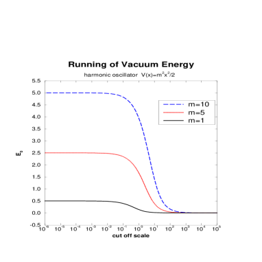
Figure 1: Running of vacuum energy

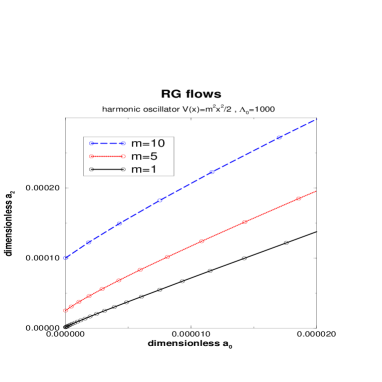
Figure 2: Flow diagram

The renormalization group flows are plotted in Fig.2 and Fig.2. We see that the momentum region where the quantum corrections are effective is finite and depends on the mass. It is the decoupling property, which enables us to get effective couplings as physical quantities even by numerical calculation within a finite momentum region.

3 Analysis of anharmonic oscillators

Now we proceed to analyze quantum mechanics of anharmonic oscillators. At first, we consider a symmetric single-well potential,

$$V_{0}(x)=~{}~{}\lambda_{0}x^{4}+\frac{1}{2}x^{2}.$$ (10)

Of course, there is no tunnelling, so our interest is to compare our NPRG results with the perturbative series. The corrected $V_{\rm eff}$ is shown in Fig.4 and we obtain the energy spectrum as in Fig.4.

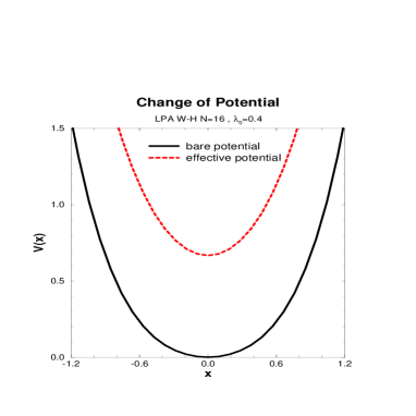
Figure 3: Change of potential

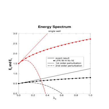
Figure 4: Energy spectrum

The perturbative series of $E_{n}$ are the asymptotic series,

$$E_{n}\!=\![n+\frac{1}{2}]+\frac{3}{4}\lambda_{0}[2n^{2}+2n+1]-\frac{1}{8}\lambda_{0}^{2}[34n^{3}+51n^{2}+59n+21]+\cdots,$$ (11)

and shows diverging nature even in the weak coupling region. Note that the Borel resummation of the perturbative series works fine in this case and gives quantitatively good values. On the other hand, even in the lowest order approximation, W-H equation can evaluate the energy spectrum almost perfectly. Therefore, NPRG could treat all orders of the perturbative series in a correct manner.

Next, we consider a symmetric double-well potential,

$$V_{0}(x)=~{}~{}\lambda_{0}x^{4}-\frac{1}{2}x^{2}.$$ (12)

In this case, there is no well-defined perturbation theory. A standard technique to get the energy gap $\Delta E$ is the dilute gas instanton calculation which gives a result with the essential singularity,

$$\Delta E=2\sqrt{\frac{2\sqrt{2}}{\pi\lambda_{0}}}e^{-\frac{1}{3\sqrt{2}\lambda_{0}}}.$$ (13)

In NPRG evolution of the effective potential, the initial double-well potential finally becomes a single well and the energy gap (mass) arises (Fig.6). This evolution is readily understandable considering that in one space-time dimension the $Z_{2}$ symmetry does not break down due to the barrier penetration, i.e. the quantum tunnelling.

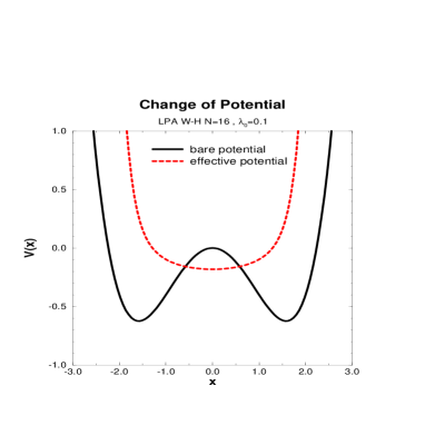
Figure 5: Change of potential

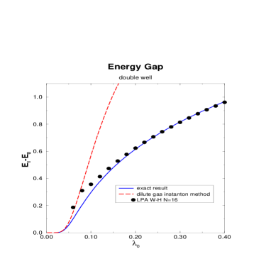
Figure 6: Energy gap

The NPRG results are very good in the strong coupling region, where we have no other method to compete (Fig.6). The perturbation can not be applied in this double-well system and the dilute gas instanton does not work at all, which is valid only in the very weak coupling region. Therefore NPRG method can be a powerful tool for analysis of tunnelling at least in such region. However, our NPRG results deviate from exact values as $\lambda_{0}\to 0$, which corresponds to a very deep well. Because the $\beta$-function becomes singular in this region, NPRG results become unreliable. We consider that the cause of difficulty comes from the approximation scheme that we now adopt. After all, the coupling regions where LPA W-H eqn. and the dilute gas instanton are valid respectively are separated completely. There is only a cross over region. In this sense, these two methods are complementary to each other.

Concerning the reliability of the results, we have to check the truncation dependence of physical quantities. In a single-well case (Fig.8), the results converge extremely well, but in a double-well case, as $\lambda_{0}$ goes smaller (Fig.8), the convergence becomes unclear. So in the small $\lambda_{0}$ region, the effective couplings at even $N=16$ are not suitable for physical quantities. We should always pay attention to the convergence with respect to $N$.[6]

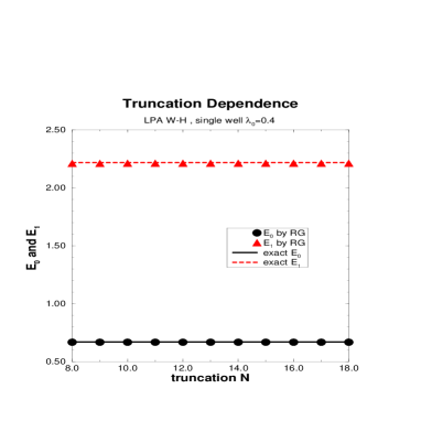
Figure 7: Single well

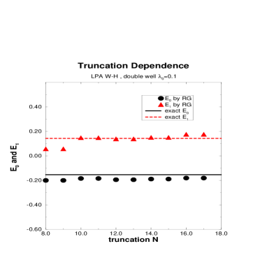
Figure 8: Double well

4 Supersymmetric quantum mechanics

Finally we analyze the supersymmetric theory, where we can see the non-perturbative dynamics of the system more clearly. We consider the Witten’s toy model for dynamical SUSY breaking[7], whose Hamiltonian is represented as follows,

$$\hat{H}=\frac{1}{2}\left[\hat{P}^{2}+\hat{W}^{2}(\Phi)+\sigma_{3}\frac{d\hat{W}(\Phi)}{d\Phi}\right]=\left(\matrix{\!\!\!\frac{1}{2}\hat{P}^{2}+\hat{V}_{+}(\Phi)~{}~{}~{}~{}~{}~{}~{}0\cr~{}~{}0~{}~{}~{}~{}~{}~{}~{}~{}~{}~{}\frac{1}{2}\hat{P}^{2}+\hat{V}_{-}(\Phi)}\right),$$ (14)

where $\hat{V}_{\pm}(\Phi)=\frac{1}{2}\hat{W}^{2}(\Phi)\pm\frac{1}{2}\frac{d\hat{W}(\Phi)}{d\Phi}$ and $\hat{W}(\Phi)$ is called SUSY potential. We define super charges $\hat{Q}_{1}=\frac{1}{2}(\sigma_{1}\hat{P}+\sigma_{2}\hat{W}(\Phi))$, $\hat{Q}_{2}=\frac{1}{2}(\sigma_{2}\hat{P}-\sigma_{1}\hat{W}(\Phi))$ and the Hamiltonian is written as $\hat{H}=\{\hat{Q}_{1},\hat{Q}_{1}\}=\{\hat{Q}_{2},\hat{Q}_{2}\}$. This assures that the vacuum energy is always non-negative, $E_{0}=\langle\Omega|\hat{H}|\Omega\rangle=2\left\|\hat{Q}_{1}|\Omega\rangle\right\|^{2}=2\left\|\hat{Q}_{2}|\Omega\rangle\right\|^{2}\geq 0$, and we have the criterion of SUSY ‘breaking’,

$$E_{0}=0\quad\Rightarrow \hat{Q}_{1}|\Omega\rangle=0,\hat{Q}_{2}|\Omega\rangle=0\qquad{\rm SUSY\quad unbroken},$$ (15)

$$E_{0}>0\quad\Rightarrow \hat{Q}_{1}|\Omega\rangle\neq 0,\hat{Q}_{2}|\Omega\rangle\neq 0\qquad{\rm SUSY\quad breaking}.$$ (16)

That is, the vacuum energy $E_{0}$ is the order parameter of SUSY ‘breaking’. Furthermore, the perturbative corrections to $E_{0}$ are vanishing in any order of perturbation, which is known as the non-renormalization theorem. Actually under the SUSY potential $W(\Phi)=g\Phi^{2}-\Phi$, $V_{+}(\Phi)$ becomes,

$$V_{+}(\Phi)=~{}~{}\frac{1}{2}g^{2}\Phi^{4}-g\Phi^{3}+\frac{1}{2}\Phi^{2}+g\Phi-\frac{1}{2},$$ (17)

and the perturbative corrections to energy spectrum are calculated as follows,

$$E_{n}=n+\frac{3}{8}g^{2}[2n^{2}+2n+1]-\frac{3}{8}g^{2}[10n^{2}+2n+1]+\cdots.$$ (18)

These corrections to $E_{0}$ are cancelled out in each order of $g$, thus there is no perturbative corrections. Namely, non-vanishing $E_{0}$ is realized only by non-perturbative effects caused by the essential singularity.

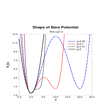
Figure 9: Bare potentials

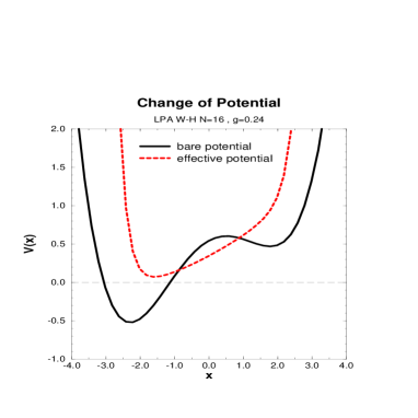
Figure 10: Change of potential

Now we analyze this system by our NPRG method. We calculate the effective potentials for a wide range of parameter $g$. The case of vanishing $g$ corresponds to the harmonic oscillator and SUSY does not break there. On the other hand, SUSY is dynamically broken at any non-vanishing $g$. Note that at small $g$ the bare potential is an asymmetric double-well, while at $g>\sqrt[4]{\frac{1}{108}}\simeq 0.31$ it is a single-well and quantum tunnelling is irrelevant there (Fig.10). Figure 10 shows the result for $g$=0.24, where the effective potential evolves into a convex one and its minimum turns out to be positive. That is, our NPRG method gives positive $E_{0}$ correctly and realizes the dynamical SUSY breaking.

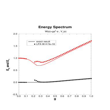
Figure 11: Energy spectrum

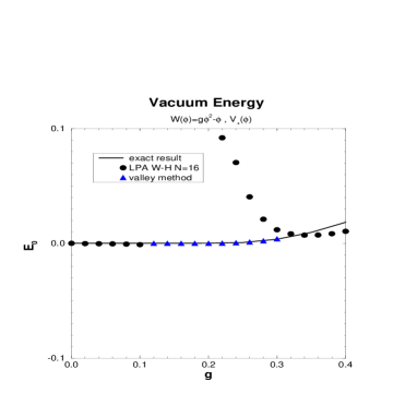
Figure 12: RG and valley instanton

As is shown in Fig.12, NPRG results are excellent in the strong coupling region, but not in the region where the bare double-well potential becomes deep. In this region ($0.1<g<0.2$), we can not show any result because of large numerical errors, while the valley instanton method works very well as shown in Fig.12. The valley instanton is generalization of the instanton method based on the valley structure of the configuration space.[8, 9] Again, two methods are somehow complementary to each other.

5 Discussions

The NPRG method, even in LPA, can evaluate the non-perturbative quantities of the summation of all orders of the perturbative series in a quantitatively good manner. As for the non-perturbative quantities characterized by the essential singularity, LPA W-H eqn. also works very well in the region where the instanton and the perturbation break down, i.e. the strong coupling region. However NPRG is not so effective in the weak coupling region because of large numerical errors. To summarize, LPA W-H eqn. and the (valley) instanton play complementary roles to each other. We don’t know the clear origin of difficulty which we encounter in our NPRG analysis. We suspect that the derivative expansion does not fit in such a parameter region. Anyway, we have to search for ‘better’ approximations.

On the other hand, from a practical point of view, NPRG method can be a good new tool for analysis of quantum tunnelling at least in some parameter region. For this purpose, we also need to study in detail how to extract tunnelling physics from the effective potential and the effective action. Those techniques may be applied to models in quantum field theories[10] and in more complex systems. Especially quantum tunnelling with multi-degrees of freedom represented by dissipation[11] is a very interesting subject to be attacked by NPRG method.

References

- [1] K.G.Wilson and J.B.Kogut, Phys.Rep. 12 (1974) 75
- [2] J.C.Le Guillou and J.Zinn-Justin (ed.), Large-Order Behaviour of Perturbation Theory, (North-Holland,1990)
- [3] S.Coleman, Aspects of symmetry,(Cambridge University Press,1985)
- [4] F.Wegner and A.Houghton, Phys.Rev. A8 (1973) 401
- [5] A.Hasenfratz and P.Hasenfratz, Nucl.Phys. B270 (1986) 687
- [6] K.-I.Aoki, K.Morikawa, W.Souma, J.-I.Sumi and H.Terao, Prog. Theor. Phys. 99 (1998) 451
- [7] E.Witten, Nucl.phys. B188 (1981) 513
- [8] H.Aoyama, H.Kikuchi, T.Harano, I.Okouchi, M.Sato and S.Wada, Prog. Theor. Phys. Supplement 127 (1997) 1
- [9] H.Aoyama, H.Kikuchi, I.Okouchi, M.Sato and S.Wada, hep-th/9808034
- [10] A.Strumia and N.Tetradis, hep-ph/9806453
- [11] A.O.Caldeira and A.J.Leggett, Ann Phys 149 (1983) 374