ITEP-TH-73/98
FISIST/16-98/CFIF

SHORT STRINGS IN THE ABELIAN HIGGS MODEL

F.V. Gubarev, M.I. Polikarpov,

Institute of Theoretical and Experimental Physics,

B. Cheremushkinskaya, 25, 117259 Moscow

E-mail: Fedor.Gubarev@itep.ru, polykarp@vxitep.itep.ru

V.I. Zakharov

Max-Planck Institut für Physik,

Föhringer Ring 6, 80805 München, Germany.

E-mail: xxz@mppmu.mpg.de

We consider the monopole-antimonopole static potential in the confining phase of the Abelian Higgs model and in particular the corrections to the Coulomb-like potential at small distances $r$. By minimizing numerically the classical energy functional we observe a linear in $r$, stringy correction even at distances much smaller than the apparent physical scales. We argue that this term is a manifestation of the condition that the monopoles are connected by a mathematically thin line along which the scalar field vanishes. These short strings modify the operator product expansion as well. Implications for QCD are discussed.

“String” or vortex-like configurations play an important role in a number of areas of physics and in theoretical speculations. The best known perhaps is the flux tube of superconductivity (“Abrikosov string”) and its relativistic version in particle physics, in the Abelian Higgs model(“Nielson-Olesen string”) [1]. Such configurations are also believed to play an important role in QCD, and the confining force between two quarks is often described as due to the stretching of the string [2].

Such physical strings have a definite thickness, reflecting the balance of the various forces going into their composition, and this introduces a certain length scale into the problem. For example for the forces between two static sources, like the quarks of QCD or between hypothetical magnetic monopoles in a superconductor, the string gives a linear potential energy at large distances, reflecting a certain energy per unit length of the string.

Naturally at small distances, that is distances small compared to the thickness of the string, where the picture of an energy per unit length does not seem to apply, we would expect the term linear in the separation to disappear. In this paper we would like to point that, surprisingly, even at small distances, that is less than the thickness of the string, there remains a stringy term in the energy. This term may be interpreted as physical manifestation of the mathematical Dirac string [3] which accompanies such objects as magnetic monopoles.

In the bulk of the paper we will consider the Abelian Higgs model (AHM) while implications for QCD are summarized in the concluding remarks. The AHM describes a gauge field $A_{\mu}$ interacting with a charged scalar field $\Phi$ as well as self-interactions of the scalar field, and the corresponding action is:

$$S=\int d^{4}x\left\{\frac{1}{4e^{2}}F^{2}_{\mu\nu}+\frac{1}{2}|(\partial-iA)\Phi|^{2}+\frac{1}{4}\lambda(|\Phi|^{2}-\eta^{2})^{2}\right\}$$ (1)

where $e$ is the electric charge, $\lambda,\eta$ are constants and $F_{\mu\nu}$ is the electromagnetic field-strength tensor, $F_{\mu\nu}\equiv\partial_{\mu}A_{\nu}-\partial_{\nu}A_{\mu}$. The scalar field condenses in the vacuum, $\langle\Phi\rangle=\eta$ and the physical vector and scalar particles are massive, $m^{2}_{V}=e^{2}\eta^{2},m_{H}^{2}=2\lambda\eta^{2}$.

The model is famous to provide with a relativistic analog of the Landau-Ginzburg theory of superconductivity. In particular, if one introduces a monopole-antimonopole pair as an external probe its static potential $V(r)$ grows linearly with the distance $r$ at large $r$:

$$lim_{r\rightarrow\infty}V(r)~{}=~{}\sigma_{\infty}r$$ (2)

The growth of the potential (2) is well understood in terms of the Abrikosov-Nielsen-Olesen (ANO) strings [1]. These strings are solutions to the classical equations of motion corresponding to the action (1) and carry (quantized) magnetic flux equal to $2\pi n/e$. Because of this, strings may end up with monopole-antimonopole pairs. The salient features of the solution is that the Higgs field $\Phi$ disappears on the axis of the string and reaches its vacuum value at transverse distances of order $1/m_{H}$ while the magnetic field extends to distances of order $1/m_{V}$. In the limit of large distances, $r\gg m_{V}^{-1},m_{H}^{-1}$ the ANO string can be considered as thin and the constant $\sigma_{\infty}$ in Eq. (2) is then its tension.

We will study the static energy of a monopole-antimonopole pair at short distances, $r\ll m_{V}^{-1},m_{H}^{-1}$. The potential $V(r)$ is then Coulomb like because of exchange of the photon. As is mentioned above, the ANO strings are not relevant at such distances, and one would expect that the power corrections to the Coulomb potential are simply due to a non-vanishing vector particle mass. That is, up to a constant which can be included into definition of the heavy masses:

$$\lim_{r\to 0}{V(r)_{Yu}}~{}\approx~{}-\frac{\alpha_{mag}}{r}\left(1+\frac{m_{V}^{2}r^{2}}{2}\right).$$

Note the change of the sign in front of the linear term as compared to the stringy potential (2).

The central point of the present letter is that these naive expectations are not true because, even at scales when the ANO string is irrelevant, there still exists an infinitely thin line inherent to the problem. Namely, there is a line connecting the monopoles along which $\Phi=0$. Its existence follows from the observation [4] that the world sheets with $\Phi=0$ are either closed or have monopole trajectories as their boundaries. In other words, it is a topological condition that magnetic charges are connected by a line $\Phi=0$, no matter how small the distance $r$ between the charges is.

Because this topological condition is so important for further results, it is worth noting that it can be rederived in the language of the Dirac string [3] as well. Namely, the infinitely thin line discussed above is nothing else but the Dirac string connecting the monopoles. The possibility of its dynamical manifestations arises from the fact that the Dirac string cannot coexist with $\Phi\neq 0$ and $\Phi$ vanishes along the string. Indeed, the self-energy of the Dirac string, is normalized to be zero in the perturbative vacuum. To justify this one can invoke duality and ask for equality of self-energies of electric and magnetic charges. Since the electric charge has no string attached the requirement would imply vanishing energy for the Dirac string. However, if the Dirac string would be embedded into a vacuum with $\langle\Phi\rangle\neq 0$ then its energy would jump to infinity since there is the term $1/2|\Phi|^{2}A_{\mu}^{2}$ in the action and $A_{\mu}^{2}\rightarrow\infty$ for a Dirac string. Hence, $\Phi=0$ along the string and it is just the condition found in [4]. In other words, Dirac strings always rest on the perturbative vacuum which is defined as a vacuum state obeying the duality principle. Therefore, even in the limit $r\to 0$ there is a deep well in the profile of the Higgs field $\Phi$. This might cost energy which is linear with $r$ even at small $r$.

By solving numerically the classical equations of motion with a boundary condition $\Phi=0$ along the line connecting the monopoles we do find a linear stringy piece, i.e. with a positive coefficient in front of $r$, in the potential even in the limit $r\to 0$. Another manifestation of the fact that we are dealing with a kind of elementary string is the breaking of the operator product expansion. Indeed the standard operator product expansion (OPE) assumes that short distance expansions can be derived in terms of exchange of elementary particles. On the other hand, the topolgical string $\Phi=0$ cannot be constructed in terms of particle exchanges but should be added independently. Since the effective string tension for small size strings is proportional to $<\Phi>^{2}$, the standard OPE breaks down at the level of $r^{2}<\Phi>^{2}$ corrections to pure perturbative results.

To evaluate the static energy $E(r)$, we first need to introduce the monopole trajectories explicitly into the path integral:

$$E(r)=\lim\limits_{T\to\infty}\left(-\frac{\partial}{\partial T}\right)\ln H(C)\,,$$ (3)

$$H(C)=\frac{\displaystyle 1}{\displaystyle Z}\int DAD\Phi[D\Phi]H(A,\Sigma^{C})e^{-S(A,\Phi)}\,,$$ (4)

here the ’t Hooft loop is defined as follows:

$$H(A,\Sigma^{C})=\exp\left\{\frac{1}{4e^{2}}\int d^{4}x\left[F^{2}_{\mu\nu}-(F_{\mu\nu}+2\pi\left[\Sigma^{C}\right]^{d}_{\mu\nu})^{2}\right]\right\}$$ (5)

where $\Sigma^{C}$ is an arbitrary surface having the contour $C$ as a boundary, $\delta\Sigma^{C}=C$. A particular form of the contour $C$ is determined by the monopoles trajectory and for a static monopole-antimonopole pair located at distance r the contour $C$ is a rectangular loop $T\times r$ with $T\gg r$. In Eq (5) $\left[...\right]^{d}$ denotes the duality operation so that for any tensor $T_{\mu\nu}$ of the second rank $\left[T_{\mu\nu}\right]^{d}=\frac{1}{2}\varepsilon_{\mu\nu\lambda\rho}\;T_{\lambda\rho}$. It can be shown that the expectation value of the ’t Hooft loop (4) does not depend on the particular choice of the surface $\Sigma^{C}$. Moreover it can be shown [5] that in the string representation of the Abelian Higgs model we have to sum over all surfaces $\sigma_{C}$ spanned on the loop $C$ and also over all closed surfaces $\sigma$ (representing virtual glueballs). The classical solution corresponds to the minimal area surface $\sigma_{C}$. Here we consider the classical approximation, hence the problem of finding $E(r)$ is equivalent to solving classical equations of motion with boundary condition $\Phi=0$ along the straight line connecting the monopoles.

Let us note that the numerical results for the potential $V(r)$ can be found in a number of papers [6, 7] and in this respect our approach is not new. However, there are no measurements dedicated specifically to small corrections to the Coulombic potential at $r\rightarrow 0$. Indeed the standard question addressed is how the Coulomb-like behaviour of the potential at short distances is transfromed into the linear potential at large distances (see, e.g., Ref. [8] and references therein). It is only very recently that it was recongnized that the power correction to the potential at short distances in QCD could signify a new phyisics [9]. Hence, there are no measurements which would provide error bars of the slope of the potential at small distances. Moreover, one could argue that at small $r$ the strong magnetic field “pushes out” the Higgs field in any case and, therefore, the potential energy is insensitive to the condition $\Phi=0$ along a line connecting the magnetic charges. Since in answering this kind of questions we rely on the numerical results, we need dedicated measurements.

We will consider the unitary gauge, $Im\Phi=0$. Then the most general ansatz for the fields consistent with the symmetries of the problem is:

$$\begin{array}[]{ll}\Phi=\eta f(\rho,z)&A_{a}=\varepsilon_{ab}\hat{x}_{b}A(\rho,z)~{}~{}~{}~{}~{}A_{0}=A_{3}=0\\ \\ \rho=[x_{a}x_{a}]^{1/2}&z=x_{3}\qquad\hat{x}_{a}=x_{a}/\rho\qquad a=1,2\ .\end{array}$$ (6)

Let us introduce also a new variable $\kappa=\sqrt{2\lambda}/e=m_{H}/m_{V}$ and measure all dimensional quantities in terms of $m_{V}=e\eta$. Then the energy functional is:

$$\begin{array}[]{l}E(r)=\frac{\pi}{e^{2}}\int\limits^{+\infty}_{-\infty}dz\int\limits^{+\infty}_{0}\rho d\rho\left\{[\frac{1}{\rho}\partial_{\rho}(\rho A)+\Sigma]^{2}+[\partial_{z}A]^{2}+\right.\\ \left.\rule{145.11052pt}{0.0pt}+[\partial_{\rho}f]^{2}+[\partial_{z}f]^{2}+f^{2}A^{2}+\frac{1}{4}\kappa^{2}(f^{2}-1)^{2}\right\}\end{array}$$ (7)

$$\Sigma=\frac{1}{\rho}\delta(\rho)\cdot\int\limits^{1}_{-1}d\xi\;\delta(z-\xi\frac{r}{2})$$ (8)

In the limit $r\to 0$ the Coulombic contribution becomes singular. The easiest way to separate the singular piece is to change the variables $A=A_{d}+a$, where $A_{d}$ is the solution in the absence of the Higgs field:

$$A_{d}=\frac{1}{2\rho}\left[\frac{z_{-}}{r_{-}}-\frac{z_{+}}{r_{+}}\right],~{}~{}~{}z_{\pm}=z\pm r/2\qquad r_{\pm}=\left[\rho^{2}+z_{\pm}^{2}\right]^{1/2}$$ (9)

Upon this change of variables the energy functional takes the form:

$$\begin{array}[]{l}E(r)=E_{self}-\pi/r+\tilde{E}(r),\\ \\ \tilde{E}(r)=\frac{\pi}{e^{2}}\int\limits^{+\infty}_{-\infty}dz\int\limits^{+\infty}_{0}\rho d\rho\left\{[\frac{1}{\rho}\partial_{\rho}(\rho a)]^{2}+[\partial_{z}a]^{2}+\right.\\ \left.\rule{145.11052pt}{0.0pt}+[\partial_{\rho}f]^{2}+[\partial_{z}f]^{2}+f^{2}(a+A_{d})^{2}+\frac{1}{4}\kappa^{2}(f^{2}-1)^{2}\right\}\end{array}$$ (10)

We investigated numerically $\tilde{E}(r)$ in the region $0.1<r<5.0$ (details of the procedure will be given elsewhere). Fig. 1 represents the results of our computations for various $\kappa$ values and clearly demonstrates that there is a linear piece in the potential even in the limit $r\ll 1$. While obtaining the values of the slope $\sigma_{0}$ at small distances we separated the Yukawa-potential contribution by fitting the energy as follows:

$$\tilde{E}_{fit}(r)=C_{0}\left(\frac{\displaystyle 1-e^{-r}}{r}-1\right)+(\sigma_{0}+\frac{1}{2}C_{0})r=\sigma_{0}r+O(r^{2})$$ (11)

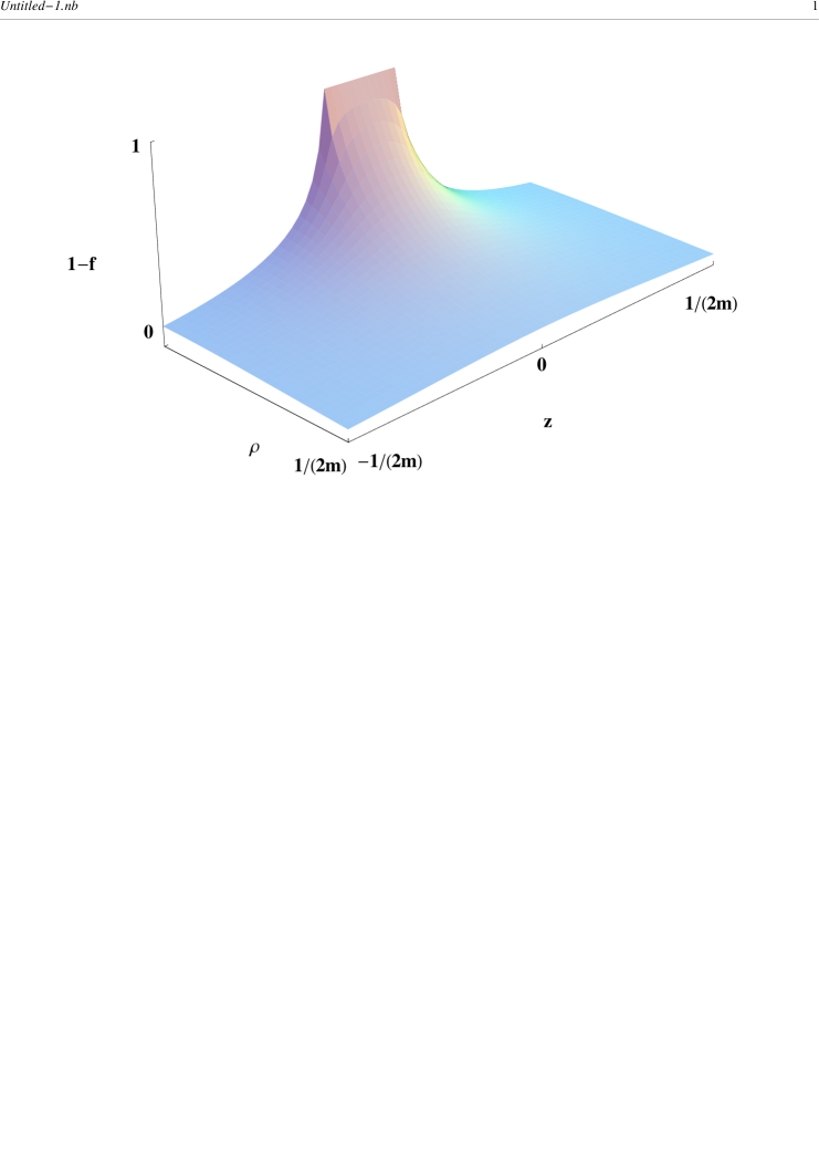
Figure 3: The function $(1-f(\rho,z))$ in the $\rho-z$ plane for $m_{H}=m_{V}=m$, $r=0.2/m$. The line at which $f=0$ is clearly seen.

The slope $\sigma_{0}$ depends smoothly on the value of $\kappa$, see Fig. 2. The linear piece in the potential at small distances reflects the boundary condition that $\Phi=0$ along the straight line connecting the monopoles. To illustrate this point we show in Fig. 3 the function $(1-f(\rho,z))$ which makes the impact of the stringy boundary condition visible. It is noteworthy that in the Bogomolny limit ($\kappa=1$) the slope of the linear potential within the error bars is the same for $r\to\infty$ and $r\to 0$.

As it is mentioned above, the existence of short strings is manifested also through breaking of the standard operator expansion. Indeed, above we found the potential in the classical approximation. In this approximation the potential is usually directly related to the propagator $D_{\mu\nu}(q^{2})$ in the momentum space,

$$V(r)=\int d^{3}r\;e^{i{\bf q\cdot r}}\;D_{00}({\bf q}^{2})$$ (12)

Moreover, as far as $q^{2}$ is in Euclidean region and much larger than the mass parameters, the propagator $D_{\mu\nu}(q^{2})$ can be evaluated by using the OPE. Restriction to the classical approximation implies that loop contributions are not included. However, vacuum fields which are soft on the scale of ${\bf q}^{2}$ can be consistently accounted for in this way (for a review of see, e.g., [10]). This standard logic can be illustrated by an example of the photon propagator connecting two electric currents. Modulus longitudinal terms, we have:

$$D_{\mu\nu}(q^{2})~{}=~{}\delta_{\mu\nu}\left({1\over q^{2}}+{1\over q^{2}}e^{2}\langle\Phi^{2}\rangle{1\over q^{2}}+{1\over q^{2}}e^{2}\langle\Phi^{2}\rangle{1\over q^{2}}e^{2}\langle\Phi^{2}\rangle{1\over q^{2}}+...\right)~{}=~{}{\delta_{\mu\nu}\over q^{2}-m_{V}^{2}}.$$ (13)

Thus, one uses first the general OPE assuming $|q^{2}|\gg e^{2}\Phi^{2}$ then substitutes the vacuum expectation of the Higgs field $\Phi$ and upon summation of the whole series of the power corrections reproduces the propagator of a massive particle. The latter can also be obtained by solving directly the classical equations of motion.

This approach fails, however, if there are both magnetic and electric charges present. In this case, one can choose the Zwanziger formalism [11] and work out an expression for propagation of a photon coupled to magnetic currents following literally the same steps as in (13), (see e.g. [12]). In the gauge $n_{\mu}D_{\mu\nu}=0$ the result is::

$$\tilde{D}_{\mu\nu}(q,n)~{}=~{}{1\over q^{2}-m_{V}^{2}}\left(\delta_{\mu\nu}-{1\over(qn)}(q_{\mu}n_{\nu}+q_{\nu}n_{\mu})+{q_{\mu}q_{\nu}\over(qn)^{2}}+{m_{V}^{2}\over(qn)^{2}}(\delta_{\mu\nu}n^{2}-n_{\mu}n_{\nu})\right).$$ (14)

Here the vector $n_{\mu}$ is directed along the Dirac strings attached to the magnetic charges and there are general arguments that there should be no dependence of physical effects on $n_{\mu}$ [11]. On the other hand, if the potential energy is given by the Fourier transform of (14) then its dependence on $n_{\mu}$ is explicit, see, e.g., [13, 14] and we addressed this problem in Ref. [5].

Note that Eq. (14) immediately implies that the standard OPE does not work any longer on the level of $q^{-2}$ corrections. Indeed, choosing $q^{2}$ large and negative does not guarantee now that the $m_{V}^{2}$ correction is small since the factor $(qn)^{2}$ in the denominator may become zero. Of course, appearance of the poles in $(qn)$ variables in longitudinal pieces is not dangerous since they drop due to the current conservation. However, the term proportional to $m_{V}^{2}$ in (14) cannot be disregarded and contribute, in particular, to (12).

The reason for the breaking of the standard OPE is that even at short distances the dynamics of the short strings should be accounted for explicitly. In particular, in the classical approximation the string lies along the straight line connecting the magnetic charges and affects the solution through the corresponding boundary condition, see above. More generally, the OPE allows to account for effect of vacuum fields, in our case for $\langle\Phi\rangle\neq 0$. The OPE is valid therefore as far as the probe particles do not change the vacuum fields drastically and the unperturbed vacuum fields are a reasonable zero-order approximation. In our case, however, the Higgs field is brought down to zero along the string and this is a nonperturbative effect. Thus, the stringy piece in the potential $V(r)$ at $r\to 0$ is a nonperturbative correction which is associated with short distances and emerges already on the classical level.

A few remarks on the implications of the results obtained to QCD are now in order. To begin with, there exist detailed numerical simulations on the lattice which confirm the dual-superconductor picture of the confinement (for review and references see [15]). In particular, the potential $V(r)$ at large $r$ is well described by the model [8]. Moreover, if the simulations are performed in the $U(1)$ projection of QCD, condensation of a scalar field $\Phi_{mag}$ with magnetic charge is confirmed and, moreover, the structure of the observed string which determines the $\bar{Q}Q$ potential at large distances is well described by the classical Landau-Ginzburg equations [16]. What is especially important for us, is that the definitions of the magnetic charges in the Abelian projection of gluodynamics [4] are in fact local and, therefore, the results obtianed within the AHM with a local field $\Phi$ can imitate gluodynamics.

Note that, naively, existence of a $U(1)$ gauge invariant operator $|\Phi_{mag}|^{2}$ of dimension $d=2$ in the abelian projection of QCD would imply infrared sensitive corrections of order $\langle\Phi_{mag}\rangle^{2}/q^{2}$ which are calculable via the OPE. On the other hand, it is well known (for references see, e.g., [10]) that such corrections are not present in QCD. The paradox is resolved through the observation that the $U(1)$ projection of QCD is similar to the Higgs model and, therefore, the OPE breaks down in this projection.

Moreover, we have learned that in the Higgs model there emerges in fact a non-perturbative short distance correction of order $q^{-2}$ manifested through the slope $\sigma_{0}\neq 0$. Although the Dirac strings are specific for the abelian projection, the results for the slope $\sigma_{0}$ which is a physical quantity should be true for any gauge fixing. In other projections, the linear potential at small distances arises if there are short-distance correlations in non-perturbative fields [9]. There are attempts to extract phenomenological consequences from hypothetical existence of short strings in QCD [20]. On the other hand, the most common picture of non-correlated finite size non-perturbative fluctuations results in $\sigma_{0}=0$ [17].

It is amusing therefore that the lattice simulation [19] do not show any change in the slope of the $\bar{Q}Q$ potential as the distances change from the largest to the smallest ones available. In the notations introduced above,

$$\sigma_{\infty}~{}\approx~{}\sigma_{0}.$$ (15)

Moreover, it is known from phenomenological analisis and from the calculations on the lattice [13, 18, 16] that the realistic QCD corresponds to the case $\kappa\approx 1$ where $\kappa=m_{H}/m_{V}$. It is remarkable that, as is mentioned above, the AHM in the classical approximation also results in the relation (15) for $\kappa\approx 1$. Thus we see that existing data [19] on the behavior of the $\bar{Q}Q$ potential at small distances agree with the classical approximation to AHM. Also, our results support indirectly phenomenological attempts to account for the novel $1/q^{2}$ corrections [20]

To summarize, we have demonstrated that the potential of a monopole-antimonopole pair at distances much smaller than the inverse masses $m^{-1}_{V,H}$ does contain a linear piece $\sigma_{0}r$ with a positive $\sigma_{0}$. This linear piece is a dynamical manifestation of the topological condition that the scalar field $\Phi$ vanishes along a line connecting the magnetic charges. These short strings are responsible also for breaking of the standard OPE on the level of $1/q^{2}$ corrections. Note that usually the Abelian Higgs model plays the role of the effective infrared model of gluodynamics (see reviews [15]). It is amusing that the behaviour of the $Q\bar{Q}$ potential at small distances obtained via the lattice simulations agree with the dual-superconductor model with $\kappa\approx 1$.

We are thankful to M.N. Chernodub, V.A. Rubakov, L. Stodolsky and T. Suzuki for interesting discussions, F.V.G. and M.I.P. feel much obliged for the kind hospitality extended to them by the staff of Max-Planck Institut fuer Physik (Munich), and by the staff of Centro de Física das Interacções Fundamentais, Edifício Ciência, Instituto Superior Técnico (Lisboa). This work was partially supported by the grants INTAS-RFBR-95-0681, INTAS-96-370, RFBR-96-15-96740 and RFBR-96-02-17230a.

Figure 1: $\frac{\displaystyle e^{2}}{\displaystyle\pi}\cdot\frac{\displaystyle E}{\displaystyle m_{v}}$ as a function of $m_{v}r$.

Figure 2: The linear slop $\sigma$ of the energy $\frac{\displaystyle e^{2}}{\displaystyle\pi}\cdot\frac{\displaystyle E}{\displaystyle m_{v}}$ in the limit $r\to 0$ as a function of $\kappa$ (see (11)).

References

-
[1]
A.A. Abrikosov, ZhETF 32 (1957) 1442;
H.B. Nielsen and P. Olesen, Nucl. Phys. B61 (1973) 45. -
[2]
Y. Nambu, Phys. Rev. D10 (1974) 4662;
G. ’t Hooft, in ”High Energy Physics”, Proc. EPS Intern. Conf., ed A. Zichichi, Editrici Compositori, (1976);
S. Mandelstam, Phys. Rep. 23 (1976) 245;
A.M. Polyakov, Phys. Lett. B59 (1975) 82. - [3] P.A.M. Dirac, Proc. Roy. Soc. A133 (1931) 60.
- [4] G. ’t Hooft, Nucl. Phys. B190 (1981) 455.
- [5] F.V. Gubarev, M.I. Polikarpov and V.I. Zakharov, Phys. Lett. B438 (1998) 147.
-
[6]
A. Jevicki and P. Senjanović, Phys. Rev.
D11 (1975) 860;
J.W. Alcock, M.J. Burfitt, and W.N. Cottingham, Nucl. Phys. B226 (1983) 299;
J.S. Ball and A. Caticha, Phys. Rev. D37 (1988) 524;
S. Kamizawa, Y. Matsubara, H. Shiba, and T. Suzuki, Nucl. Phys. B389 (1993) 563;
M. Baker, N. Brambilla, H. G. Dosch and A. Vairo, Phys.Rev. D58 (1998) 034010. - [7] S. Maedan, Y. Matsubara and T. Suzuki, Progr. Theor. Phys. 84 (1990) 130.
- [8] M. Baker, J.S. Ball, N. Brambila, C.M. Prosperi, F Zachariasen, Phys. Rev. 54 (1996) 2829.
- [9] R. Akhoury and V.I. Zakharov, Phys. Lett. B438 (1998) 165.
- [10] V.A. Novikov et.al., Fortsch. Phys. 32 (1985) 585.
- [11] D. Zwanziger, Phys. Rev. D3 (1971) 343.
- [12] A.P. Balachandran, H. Rupertsberger, J. Schechter, Phys. Rev. D11 (1975) 2260.
- [13] T. Suzuki, Progr. Theor. Phys. 80 (1988) 929, ibid 81 (1989) 752;
- [14] S. Sasaki, H. Suganuma, H. Toki, ibid 94 (1995) 384.
-
[15]
M. N. Chernodub and M. I. Polikarpov,
Lectures given at the Workshop “Confinement,
Duality and Non-Perturbative Aspects of QCD”, Cambridge (UK),
24 June - 4 July 1997, hep-th/9710205;
G. S. Bali, Talk given at 3rd International Conference on Quark Confinement and the Hadron Spectrum (Confinement III), Newport News, VA, 7-12 Jun 1998, hep-ph/9809351. - [16] G.S. Bali, C. Schlichter, K. Schilling, Prog.Theor.Phys.Suppl. 131 (1998) 645-656.
-
[17]
Ya.Ya. Balitskii, Nucl. Phys. B254 (1985) 166;
H.G. Dosh and Yu.A. Simonov, Phys. Lett. B205 (1988) 339. -
[18]
M. Baker, J. S. Ball and F. Zachariasen, Phys.Rev.
D41 (1990) 2612;
V. Singh, R. Haymaker and D. Browne, Phys.Rev. D47 (1993) 1715;
Y. Matsubara, S. Ejiri and T. Suzuki, Nucl.Phys.Proc.Suppl. 34 (1994) 176;
S. Kato et al, it Nucl.Phys.Proc.Suppl. 63 (1998) 471;
- [19] G.S. Bali, K. Schilling, A. Wachter, hep-lat/9506017; Phys. Rev. D55 (1997) 5309.
-
[20]
K.G. Chetyrkin, S. Narison and V.I. Zakharov,
hep-ph/9811275;
V.I. Zakharov, hep-ph/9802416.