Abstract

We begin a classification of the symmetry algebras arising on configurations of type IIB $[p,q]$ 7-branes. These include not just the Kodaira symmetries that occur when branes coalesce into a singularity, but also algebras associated to other physically interesting brane configurations that cannot be collapsed. We demonstrate how the monodromy around the 7-branes essentially determines the algebra, and thus 7-brane gauge symmetries are classified by conjugacy classes of the modular group $SL(2,{\sf Z\!\!\!Z})$. Through a classic map between the modular group and binary quadratic forms, the monodromy fixes the asymptotic charge form which determines the representations of the various $(p,q)$ dyons in probe D3-brane theories. This quadratic form also controls the change in the algebra during transitions between different brane configurations. We give a unified description of the brane configurations extending the $D_{N}$, $E_{N}$ and Argyres-Douglas $H_{N}$ series beyond the Kodaira cases. We anticipate the appearance of affine and indefinite infinite-dimensional algebras, which we explore in a sequel paper.

1 Introduction

Over the last couple of years F-theory [1] compactifications on an elliptic K3 have been studied explicitly as type IIB compactifications involving of $[p,q]$ 7-branes. In particular, an elliptic K3 with a Kodaira singularity maps to a 7-brane configuration where the branes have coalesced to form the singularity. It has become clear, however, that the Kodaira singularities do not exhaust the set of 7-branes configurations relevant to field theory applications. There exist 7-brane configurations that cannot be collapsed, but nevertheless provide backgrounds for interesting D3-brane probe theories. The most familiar examples of such theories are the ${\cal N}=2$, $D=4$ Seiberg-Witten theories [2] with $N_{f}\leq 3$ flavors. These can be realized in the presence of background 7-brane configurations of $D_{N_{f}}$ global symmetry type, but the branes cannot be collapsed since Kodaira singularities of $D_{N}$ type only appear for $N\geq 4$. Other examples include the four-dimensional theories with $E_{N}$ global symmetry, where any value $N\geq 0$ arises from a possible 7-brane background configuration, but only for $N=5,6,7,8$ the 7-branes can be collapsed to a singularity.

These applications, as well as others, have led us to consider enumerating all the possible 7-brane configurations and their corresponding algebras, whether or not there is an associated singularity. Finite Lie algebras arising on 7-brane configurations were explored in [3, 4, 5, 6, 7], and it was shown in detail how $(p,q)$ strings and string junctions stretched between the 7-branes correspond to vector bosons of the eight-dimensional gauge theory. In M-theory these junctions lift to M2-branes embedded in K3, and the requirement that the states be BPS specifies that these branes must be holomorphically embedded, i.e. they are wrapped on holomorphic 2-cycles of the K3 [8]. An inner product on junction space is induced from the intersection of the associated 2-cycles, and the Cartan matrix of the Lie algebra appears as the intersection matrix of a basis of string junctions ending on the 7-brane configuration. The algebra is then realized on the branes through the composition of junctions. A key result of [7] was the expression of the self-intersection of a junction emerging from a 7-brane configuration with “asymptotic” charges $(p,q)$,

$$\mbox{\boldmath$\bf J$}^{2}=-\lambda\cdot\lambda+f\,(p,q)\,,$$ (1.1)

where $\lambda$ is the Lie algebra weight vector associated to the junction and $f(p,q)$ is a quadratic form determined by the 7-brane configuration.

The requirement of holomorphy implies a constraint on the self-intersection of a junction, and this was exploited in [9] to determine the possible BPS junctions on theories with a single probe D3-brane in a 7-brane background. The BPS spectra of $SU(2)$ Seiberg-Witten theory for $N_{f}\leq 4$ was reproduced exactly using only this constraint. (A related constraint was used to obtain the $N_{f}=0$ case in [8].) Results were derived for the largely unknown spectra of the four-dimensional theories with $E_{N}$ global symmetry. Much about their spectra is controlled by the quadratic form $f(p,q)$ appearing in (1.1). The computation of self-intersection for junctions for the case of 7-brane backgrounds and multiple D3-branes was given in [10].

In this paper we expand on and systematize this previous work. We begin a classification of all the possible configurations of 7-branes, and their associated algebras. We find that the monodromy matrix associated to a set of 7-branes essentially specifies which Lie algebra is realized. More precisely, in all cases we have considered, the $SL(2,{\sf Z\!\!\!Z})$ conjugacy class of the monodromy, together with the number of branes and an integer $\ell$ characterizing the possible asymptotic charges of junctions, determine the algebra uniquely.

Thus we find an elegant organization of all possible Lie algebras on 7-branes based on conjugacy classes of $SL(2,{\sf Z\!\!\!Z})$ matrices. The classification of such conjugacy classes is a well-known mathematical problem closely related to the classification of equivalence classes of binary quadratic forms. This relation is implemented by a map associating binary quadratic forms to elements of $SL(2,{\sf Z\!\!\!Z})$. According to the value of its trace, an $SL(2,{\sf Z\!\!\!Z})$ matrix is either elliptic, parabolic or hyperbolic. We find that the finite algebras corresponding to Kodaira singularities exhaust the elliptic classes and fill some of the parabolic classes, while the other non-collapsible finite algebra configurations are in parabolic classes and hyperbolic classes of negative trace.

Although the conjugacy classes of $SL(2,{\sf Z\!\!\!Z})$ matrices are the primary organizational tool, the classification also requires the number of branes and the integer $\ell$, and perhaps other data we have not yet encountered. Specifying the number of branes is necessary because there exist configurations of twelve branes with unit monodromy, which nonetheless change the algebra of a given configuration considerably. When different from one, $\ell$ indicates that not all possible asymptotic charges can appear on junctions. We have found configurations that have the same monodromy and the same number of branes but give different algebras; in such cases $\ell$ differs. Similarly, configurations with the same algebras and number of branes will have inequivalent monodromies if $\ell$ is distinct.

We also show that the map from $SL(2,{\sf Z\!\!\!Z})$ to quadratic forms, applied to the monodromy matrix of the brane configuration, gives us the corresponding asymptotic charge quadratic form $f(p,q)$ appearing in (1.1). We explore systematically how this quadratic form controls the change in the Lie algebra when a new brane is introduced. We find that $f(p,q)$, where $f$ is the asymptotic charge form for the original configuration and $[p,q]$ are the charges of the new brane, precisely encodes the type of enhancement that takes place. When $f(p,q)<-1$ the original algebra is only supplemented by a new $u(1)$, while for precisely $f(p,q)=-1$ an additional $A_{1}$ appears. For values $-1<f(p,q)<1$, the original algebra enhances to some other finite algebra with rank greater by one.

We also present a simple and unified description of the ${\bf D_{N}}$, ${\bf E_{N}}$ and ${\bf H_{N}}$ series of configurations, which realize $D_{N}$, $E_{N}$ and $A_{N}$ algebras respectively. These configurations can collapse into Kodaira singularities for ${\bf D_{N}}$, $N\geq 4$, for ${\bf E_{5}}$, ${\bf E_{6}}$, ${\bf E_{7}}$ and ${\bf E_{8}}$, and finally for ${\bf H_{0}}$, ${\bf H_{1}}$ and ${\bf H_{2}}$, the configurations associated to Argyres-Douglas points. The configurations ${\bf D_{5}}$ and ${\bf E_{5}}$ both realize a $D_{5}$ algebra, and as an example we show explicitly how one configuration can be transformed into the other by a global $SL(2,{\sf Z\!\!\!Z})$ transformation and by relocation of branch cuts.

Once one considers brane configurations that are not collapsible, infinite-dimensional algebras appear naturally. This was seen in [11], where it was shown that affine Lie algebras arise whenever the junction intersection form produces an affine Cartan matrix. We discuss how these and other infinite-dimensional Lie algebras appear in our classification, filling many of the remaining $SL(2,{\sf Z\!\!\!Z})$ conjugacy classes and corresponding to brane transitions with $f(p,q)\geq 1$, in the sequel paper [12].

In the present paper we also take the opportunity to discuss explicitly a basic issue that is seldom brought into the open. We explain in general terms how a Lie algebra arises from BPS junctions (or holomorphic 2-cycles). The conventional wisdom is that once the intersection matrix of a set of basis junctions gives the Cartan matrix of a Lie algebra, that algebra is realized. We give evidence for this idea by showing that when a set of junctions represent simple roots, namely, their intersections define a Cartan matrix, the constraints of holomorphicity applied to junctions built from these basis junctions naturally take the form of Serre relations. These relations indeed constrain the combinations of simple roots that define allowed roots in the Chevalley-Serre construction of a Lie algebra starting from a Cartan matrix. We also indicate what aspects of the construction survive when the algebra to be identified has no Cartan matrix, or when we deal with nontrivial infinite dimensional algebras.

This paper is organized as follows. In section 2 we show how to compute efficiently monodromies and their traces. We define carefully the notion of equivalent brane configurations, illustrating it with examples. We also consider explicitly the classification of configurations with two 7-branes. In section 3 we begin by explaining how a Lie algebra arises from junctions. We then show how the monodromy of a configuration determines the associated charge quadratic form, and prove a relation between the trace of the monodromy and the determinant of the Cartan matrix associated to the algebra arising from the brane configuration. In section 4 we consider the unified presentation and extension of the main Kodaira series, as well as generalizations thereof. In sections 5 and 6 we discuss transitions between brane configurations, limiting ourselves to the case when the resulting algebra is finite. In section 7 we collect the results relevant to the general classification of brane configurations, anticipating some of the results to be explained in [12].

2 7-Brane Configurations and Monodromies

In this section we first discuss a few simple computations involving branes and their monodromies. These include $SL(2,{\sf Z\!\!\!Z})$ conjugation, computations of traces, and transformations induced by moving branch cuts. We then explain in detail our notion of equivalent brane configurations. This notion is illustrated with some examples. One noteworthy example also illustrates an exception, namely that in the exceptional series $E_{N}$ there are two inequivalent brane configurations associated to $E_{1}$. Finally, we discuss a classification of brane configurations involving two 7-branes.

2.1 Monodromy matrices and moving branch cuts

Throughout the paper we shall be considering configurations of IIB 7-branes, filling (7+1) dimensions and pointlike in the remaining two, which we take to be the complex plane. These 7-branes are magnetic sources for the complex dilaton-axion scalar $\tau=\chi+ie^{-\phi}$. This scalar experiences a monodromy around each 7-brane, which we account for by introducing a branch cut associated to each 7-brane. Following the conventions of [5, 7], a generic background is specified by listing the 7-branes in the order in which their branch cuts are crossed when encircling them in a counterclockwise direction.

A 7-brane is labeled by two relatively prime integers $(p,q)$ up to a sign; a $[p,q]$ 7-brane is the same object as a $[-p,-q]$ 7-brane. It is convenient to place the branes in a canonical presentation, locating them along the real axis, ordered from left to right and with the cuts going downwards. When crossing the cut of an individual $[p,q]$-brane, $\tau$ transforms with the $SL(2,{\sf Z\!\!\!Z})$ monodromy matrix $K_{[p,q]}$ [13]. It is convenient to unify the two charges in a vector ${\bf z}=({p\atop q})$, in terms of which $K_{\bf z}$ is given as

$$K_{\bf z}=1\!\!1+{\bf z}{\bf z}^{T}S = \left(\begin{array}[]{cc}1+pq&-p^{2}\\ q^{2}&1-pq\end{array}\right)\,,$$ (2.4)

where $S\equiv\pmatrix{0&-1\cr 1&0}$. Under the operation of global $SL(2,{\sf Z\!\!\!Z})$ conjugation with an element $g$ one finds

$$g\,K_{\bf z}\,g^{-1}=K_{g\,{\bf z}}\,.$$ (2.5)

Following the conventions stated above, the total monodromy around the brane configuration $\mbox{\boldmath$\bf X$}_{1}\ldots\mbox{\boldmath$\bf X$}_{n-1}\mbox{\boldmath$\bf X$}_{n}\,,$ is given by

$$K=K_{{\bf z}_{n}}K_{{\bf z}_{n-1}}\ldots K_{{\bf z}_{1}}\,,$$ (2.6)

and will be of vital importance to us. The labeling of branes actually depends on the placement of branch cuts. We can move the branch cut of one 7-brane $\mbox{\boldmath$\bf X$}_{{\bf z}_{1}}$ across another 7-brane $\mbox{\boldmath$\bf X$}_{{\bf z}_{2}}$, thus changing the latter to $\mbox{\boldmath$\bf X$}_{{\bf z}^{\prime}_{2}}$ and exchanging their order in the canonical presentation, or we can move the cut of $\mbox{\boldmath$\bf X$}_{{{\bf z}_{2}}}$ across $\mbox{\boldmath$\bf X$}_{{\bf z}_{1}}$. This was explained in [5], and the result can be written as follows:

$${\bf X}_{\displaystyle{\bf z}_{1}}{\bf X}_{\displaystyle{\bf z}_{2}} = {\bf X}_{\displaystyle{\bf z}_{2}}\,{\bf X}_{\,\displaystyle({\bf z}_{1}+({\bf z}_{1}\times{\bf z}_{2})\,{\bf z}_{2}\,)}$$ (2.7)

$$= {\bf X}_{\,\displaystyle({\bf z}_{2}+({\bf z}_{1}\times{\bf z}_{2})\,{\bf z}_{1}\,)}\,{\bf X}_{\displaystyle{\bf z}_{1}}\,,$$

where we have defined

$${\bf z}_{1}\!\times\!{\bf z}_{2}\equiv-{\bf z}_{1}^{T}S\,{\bf z}_{2}={\bf z}_{2}^{T}S\,{\bf z}_{1}=\hbox{det}\,\pmatrix{p_{1}&p_{2}\cr q_{1}&q_{2}}\,.$$ (2.8)

Equation (2.7) indicates the fixed brane acquires an extra charge equal to the charge of the moving brane times the determinant of the relative charges.

For a given brane configuration the trace of the associated monodromy is an $SL(2,{\sf Z\!\!\!Z})$ invariant. Given the configuration ${\mbox{\boldmath$\bf X$}_{1}\mbox{\boldmath$\bf X$}_{2}\cdots\mbox{\boldmath$\bf X$}_{n}}$ with monodromy $K=K_{n}\cdots K_{2}K_{1}$ the trace of $K$ is calculated using (2.4). One finds:

$$\hbox{Tr}\,K=2+\sum_{k=2}^{n}\,\,\,\,\,\,\,\,\!\!\!\!\!\!\sum_{i_{1}<i_{2}\ldots<i_{k}}({\bf z}_{i_{1}}\!\times\!{\bf z}_{i_{2}})({\bf z}_{i_{2}}\!\times\!{\bf z}_{i_{3}})\ldots({\bf z}_{i_{k}}\!\times\!{\bf z}_{i_{1}}).$$ (2.9)

Another useful $SL(2,{\sf Z\!\!\!Z})$ invariant of a brane configuration $\mbox{\boldmath$\bf X$}_{1}\mbox{\boldmath$\bf X$}_{2}\ldots\mbox{\boldmath$\bf X$}_{n}$ is the positive integer $\ell$, the greatest common divisor of all non-vanishing pairwise determinants:

$$\ell\equiv\left\{\begin{array}[]{ll}\gcd\{{\bf z}_{i}\times{\bf z}_{j},\mbox{for all $i,j$}\;\}&\mbox{for mutually nonlocal branes}\\ 0&\mbox{for mutually local branes}.\end{array}\right.$$ (2.10)

For reasons that will be explained at the beginning of sect. 3, we sometimes call $\ell$ the asymptotic charge invariant. It is manifest that $\ell$ is invariant under global $SL(2,{\sf Z\!\!\!Z})$ transformations, and it can be shown it also does not change when branch cuts are relocated.

In this paper we continue to label some useful branes in the way we did in previous works. We take $\mbox{\boldmath$\bf A$}={\bf[1,0]}$ ($K_{\bf A}=T^{-1}$), $\mbox{\boldmath$\bf B$}={\bf[1,-1]}$ ($K_{\bf B}=ST^{2}$), and $\mbox{\boldmath$\bf C$}={\bf[1,1]}$ ($K_{\bf C}=T^{2}S$). Branes of other charges ${\bf z}$ will be denoted by $\mbox{\boldmath$\bf X$}_{{\bf z}}$.

2.2 Equivalence classes of brane configurations

The classification of the algebras that can arise on configurations of 7-branes has to take into account equivalence transformations between different configurations. We define:

Two 7-brane configurations will be said to be equivalent (indicated as $\cong$) if they have the same number of branes and their canonical presentations can be matched brane by brane using the operations of overall $SL(2,{\sf Z\!\!\!Z})$ conjugation and relocation of branch cuts.

Global $SL(2,{\sf Z\!\!\!Z})$ conjugation changes some brane labels and may or may not change the overall monodromy. Due to the $SL(2,{\sf Z\!\!\!Z})$ symmetry of type IIB string theory, it does not change the physics and is therefore an equivalence transformation when applied to a complete configuration. Moving branch cuts, as reviewed in the previous subsection, does not change the overall monodromy, only the labels of the individual 7-branes. Two brane configurations related only by relocation of branch cuts will be said to be equal.

Brane configurations can only be equivalent if their monodromies are conjugate in $SL(2,{\sf Z\!\!\!Z})$. In addition, they must have the same value of the invariant $\ell$. In all the examples we have studied, we have found that two configurations with conjugate monodromies, equal values for $\ell$ and the same number of branes are equivalent. Although we have no general proof, we conjecture that

Conjecture: Inequivalent 7-brane configurations are classified by monodromy, number of branes and the asymptotic charge invariant $\ell$.

Classifying equivalence classes of monodromies in $SL(2,{\sf Z\!\!\!Z})$ is a well-studied but complicated problem. It is useful to consider the trace of the monodromy, which is an $SL(2,{\sf Z\!\!\!Z})$ invariant. Two monodromies with different trace are necessarily inequivalent, but if their traces agree they still need not be equivalent. Indeed, there are inequivalent conjugacy classes in $SL(2,{\sf Z\!\!\!Z})$ with the same trace.

In the remainder of this section, we will work through an example of brane configurations that are equivalent, and we prove this completely by mapping the brane configurations into each other explicitly. Another similar example is given in the sequel paper [12]. Following this we present two different series realizing the $E_{N}$ algebras, and prove the equivalence of all pairs in the two series except for one pair, having to do with $E_{1}$. This exception illustrates how differing $\ell$ can render configurations inequivalent.

Equivalence of two realizations of so(10). Consider the conventional ${\bf D_{5}}=\mbox{\boldmath$\bf A$}^{5}\mbox{\boldmath$\bf B$}\mbox{\boldmath$\bf C$}$ configuration of branes known to give the $D_{5}=so(10)$ algebra. On the other hand the $E_{5}$ algebra of the exceptional series is isomorphic to $D_{5}$. Since $E_{6}$, $E_{7}$ and $E_{8}$ are realized on ${\bf E_{6}}=\mbox{\boldmath$\bf A$}^{5}\mbox{\boldmath$\bf B$}\mbox{\boldmath$\bf C$}\mbox{\boldmath$\bf C$}$, ${\bf E_{7}}=\mbox{\boldmath$\bf A$}^{6}\mbox{\boldmath$\bf B$}\mbox{\boldmath$\bf C$}\mbox{\boldmath$\bf C$}$, and ${\bf E_{8}}=\mbox{\boldmath$\bf A$}^{7}\mbox{\boldmath$\bf B$}\mbox{\boldmath$\bf C$}\mbox{\boldmath$\bf C$}$, it is natural to ask whether the brane configuration ${\bf E_{5}}=\mbox{\boldmath$\bf A$}^{4}\mbox{\boldmath$\bf B$}\mbox{\boldmath$\bf C$}\mbox{\boldmath$\bf C$}$ gives an equivalent construction of $so(10)$. The answer is yes. To show this we first confirm that the two monodromies are $SL(2,{\sf Z\!\!\!Z})$ conjugate

$$K({\bf E_{5}})=-K_{\bf[1,1]}=\left(\begin{array}[]{cc}-2&1\\ -1&0\end{array}\right)\sim\left(\begin{array}[]{cc}-1&1\\ 0&-1\end{array}\right)=-K_{\bf[1,0]}=K({\bf D_{5}})\,.$$ (2.11)

The $SL(2,{\sf Z\!\!\!Z})$ transformation can be taken to be the transformation that acting on the $[1,0]$ brane gives the $[1,1]$ brane

$$K_{\bf[1,1]}=g\,K_{\bf[1,0]}\,\,g^{-1}\,,\qquad g=\pmatrix{1&0\cr 1&1},$$ (2.12)

for example. This transformation turns $\mbox{\boldmath$\bf A$}^{5}\mbox{\boldmath$\bf B$}\mbox{\boldmath$\bf C$}$ into $\mbox{\boldmath$\bf C$}^{5}\mbox{\boldmath$\bf A$}\mbox{\boldmath$\bf X$}_{\bf[1,2]}$. This configuration must now be shown to be identical to $\mbox{\boldmath$\bf A$}^{4}\mbox{\boldmath$\bf B$}\mbox{\boldmath$\bf C$}\mbox{\boldmath$\bf C$}$ by moving cuts. By repeated use of eqn. (2.7) we find the claimed equivalence:

$$\mbox{\boldmath$\bf C$}^{5}\mbox{\boldmath$\bf A$}\,\mbox{\boldmath$\bf X$}_{\bf[1,2]} = \mbox{\boldmath$\bf A$}\,(\mbox{\boldmath$\bf X$}_{\bf[0,1]})^{5}\,\mbox{\boldmath$\bf X$}_{\bf[1,2]}=\mbox{\boldmath$\bf A$}\,(\mbox{\boldmath$\bf X$}_{\bf[0,1]})^{4}\,(\mbox{\boldmath$\bf X$}_{\bf[0,1]}\mbox{\boldmath$\bf X$}_{\bf[1,2]})=\mbox{\boldmath$\bf A$}\,(\mbox{\boldmath$\bf X$}_{\bf[0,1]})^{4}\,\mbox{\boldmath$\bf C$}\,\mbox{\boldmath$\bf X$}_{\bf[0,1]}$$

$$= \mbox{\boldmath$\bf A$}\,(\mbox{\boldmath$\bf X$}_{\bf[0,1]})^{2}\,\mbox{\boldmath$\bf C$}\,\mbox{\boldmath$\bf A$}^{2}\,\mbox{\boldmath$\bf X$}_{\bf[0,1]}=\mbox{\boldmath$\bf A$}\,(\mbox{\boldmath$\bf X$}_{\bf[0,1]})^{2}\,\mbox{\boldmath$\bf A$}^{2}\,\mbox{\boldmath$\bf B$}\,\mbox{\boldmath$\bf X$}_{\bf[0,1]}$$

$$= \mbox{\boldmath$\bf A$}\,((\mbox{\boldmath$\bf X$}_{\bf[0,1]})^{2}\,\mbox{\boldmath$\bf A$})\,\mbox{\boldmath$\bf A$}\,(\mbox{\boldmath$\bf B$}\,\mbox{\boldmath$\bf X$}_{\bf[0,1]})=\mbox{\boldmath$\bf A$}^{2}\mbox{\boldmath$\bf B$}^{2}\mbox{\boldmath$\bf A$}^{2}\mbox{\boldmath$\bf B$}$$

$$= \mbox{\boldmath$\bf A$}^{4}\,(\mbox{\boldmath$\bf X$}_{\bf[3,-1]})^{2}\,\mbox{\boldmath$\bf B$}=\mbox{\boldmath$\bf A$}^{4}\mbox{\boldmath$\bf B$}\mbox{\boldmath$\bf C$}\mbox{\boldmath$\bf C$}\,.$$

Equivalence and inequivalence in the $E_{N}$-series. We now examine two series of algebras which realize the $E_{N}$ algebras, ${\bf E_{N}}={\bf A}^{N-1}{\bf BCC}$ and ${\bf\tilde{E}_{N}}={\bf A}^{N}{\bf X}_{\bf[2,-1]}{\bf C}$. The first is a familiar series [3, 4], while the second will be introduced and explained in section 4.

Note that the second series gives a definition for ${\bf E_{0}}$ as $\mbox{\boldmath$\bf X$}_{\bf[2,-1]}\mbox{\boldmath$\bf C$}$ while the first series does not. The two series are equivalent for  $N\geq 2$. To prove this it is enough to concentrate on the four rightmost branes:

$${\bf ABCC}={\bf BX}_{\bf[0,1]}{\bf CC}={\bf BAAX}_{\bf[0,1]}={\bf AAX}_{\bf[3,-1]}{\bf X}_{\bf[0,1]}\stackrel{{\scriptstyle K_{A}^{-1}}}{{\cong}}{\bf AAX}_{\bf[2,-1]}{\bf C},$$ (2.14)

where the last step involves conjugation with $K_{A}$, which does not affect the rest of the spectator A-branes. The steps in (2.14), however, cannot be applied to the case of fewer then four branes. This means that ${\bf E_{1}}={\bf BCC}$ and ${\bf\tilde{E}_{1}}={\bf AX_{\bf[2,-1]}}{\bf C}$ need not be equivalent. In fact, they are not. We readily find from (2.10) that $\ell({\bf E_{1}})=2$, while $\ell({\bf\tilde{E}_{1}})=1$, thus guaranteeing inequivalence. Note that $\ell({\bf E_{N}})=1$ for $N\geq 2$.

3 String Junctions, Lie Algebras and Quadratic Forms

Thus far we have discussed only the $[p,q]$ 7-branes themselves. Configurations of 7-branes support strings and string junctions stretched in between them. There exist BPS junctions realizing the adjoint of the 7-brane algebra ${\cal G}$, and in the case of ${\cal G}$ finite they are gauge bosons living on the 7-brane worldvolume theory, as we now review.

The labels $(p,q)$ are also associated to segments of strings corresponding to bound states of fundamental and D-strings [14]. In crossing the branch cut of an $[r,s]$ 7-brane in the counterclockwise direction, the $(p,q)$ charges of a string segment change as $({p\atop q})\rightarrow K_{[r,s]}\,({p\atop q})$. Under global $g\in SL(2,{\sf Z\!\!\!Z})$ transformations all charges carried by strings change as $({p\atop q})\rightarrow g\,({p\atop q})$. A $(p,q)$ string can end only on a $[p,q]$ 7-brane, a statement that is $SL(2,{\sf Z\!\!\!Z})$-invariant as 7-brane labels $[r,s]$ change as $({r\atop s})\rightarrow g\,({r\atop s})$, as well as invariant under moving branch cuts.

A web of $(p,q)$-strings, here called a junction, is charged under the $u(1)$ gauge field of a given 7-brane $\bf X$ if the associated invariant charge $Q_{\bf X}$ defined in [7] is non-vanishing. This charge combines the contribution from crossing the cut of $\bf X$ and the contribution of string prongs emanating from $\bf X$ in a way that is invariant under Hanany-Witten transformations [15]. We call two junctions equivalent if they are related by junction transformations as defined in [7, 16]; it was proven in [16] that the BPS representative of an equivalence class of junctions containing an open string is unique. The algebraic properties of a given string junction are entirely specified by the set of invariant charges $\{Q_{\bf X}{{}_{i}}\}$, where $\mbox{\boldmath$\bf X$}_{i}$, $i=1\ldots n$, are the set of 7-branes. From now on we shall refer to an equivalence class of junctions simply as a junction, and denote it as $\bf J$. Thus the space of junctions is a lattice of dimension equal to the number of branes, with a junction $\bf J$ expressed as

$$\mbox{\boldmath$\bf J$}=\sum_{i=1}^{n}\,Q_{{\bf X}_{i}}\,\mbox{\boldmath$\bf x$}_{i}\equiv Q^{\mu}\,\mbox{\boldmath$\bf x$}_{\mu}\,,$$ (3.15)

where $\mu$ indexes the branes and the “basis strings” $\mbox{\boldmath$\bf x$}_{\mu}$ can be thought of as a basis of string prongs leaving each brane.

A given junction will carry some total amount of $p$ and $q$ charges away from the 7-brane configuration; we call these the asymptotic charges of the junction. The integer $\ell$ introduced in (2.10) constrains the possible asymptotic charges that can be realized on junctions in a given 7-brane configuration. Let ${\bf z}=({p\atop q})$ denote the asymptotic charges of a junction emerging from a configuration, and let ${\bf z}_{i}=({p_{i}\atop q_{i}})$ denote the brane charges in the configuration.

The constraint takes the form

$${\bf z}\times\,{\bf z}_{i}=0\,(\hbox{mod}\,\ell)\,\,,$$ (3.16)

for every ${\bf z}_{i}$ in the brane configuration. Indeed, any emerging junction must have ${\bf z}=\sum_{i}n_{i}{\bf z}_{i}$ for integers $n_{i}$, and then (3.16) follows immediately from the definition (2.10). In fact, one need only check (3.16) for a single brane ${\bf z}_{i}$ of the configuration; if ${\bf z}\times\,{\bf z}_{i}$ and ${\bf z}_{i}\times\,{\bf z}_{j}$ vanish mod$(\ell)$, then ${\bf z}\times\,{\bf z}_{j}$ will also vanish mod$(\ell)$.

Instead of using invariant charges as in (3.15), we can specify a junction with a Lie algebra weight vector $\lambda=a_{i}\,\omega^{i}$, and asymptotic charges $p$, $q$:

$$\mbox{\boldmath$\bf J$}=\sum_{i}a_{i}\,\mbox{\boldmath$\bf\omega$}^{i}+p\,\mbox{\boldmath$\bf\omega$}^{p}+q\,\mbox{\boldmath$\bf\omega$}^{q}\,,$$ (3.17)

where the $\mbox{\boldmath$\bf\omega$}^{i}$ are $n-2$ junctions of zero asymptotic charge representing the weights of the algebra, and $\mbox{\boldmath$\bf\omega$}^{p}$ and $\mbox{\boldmath$\bf\omega$}^{q}$ are Lie algebra singlets with asymptotic charges $(1,0)$ and $(0,1)$ respectively. The $a_{i}$ and $p,q$ are linear combinations of the $Q_{\bf X}{{}_{i}}$.

In a few cases, the Lie algebra is not semisimple, but consists of a semisimple part of rank $r$ and a number of $u(1)$ factors. In this case the $(n-2)$ Dynkin labels are replaced by $r$ Dynkin labels and $((n-2)-r)$ $u(1)$ charges in a generalized weight vector. For simplicity of notation, we denote all these charges by $a_{i}$. The asymptotic charges $p$ and $q$, however, are not considered $u(1)$ charges. The $\mbox{\boldmath$\bf\omega$}^{i}$ associated to $u(1)$ charges will not be true Lie algebraic fundamental weights, but will just be some basis junctions with zero asymptotic charge. Similarly, their duals $\mbox{\boldmath$\bf\alpha$}_{i}$ will not be true simple roots, but will obey $(\mbox{\boldmath$\bf\alpha$}_{i},\mbox{\boldmath$\bf\alpha$}_{i})<2$; as we shall see shortly, this means they are not BPS, but they are still useful as basis junctions.

Furthermore, note that $\mbox{\boldmath$\bf\omega$}^{i},\mbox{\boldmath$\bf\omega$}^{p},\mbox{\boldmath$\bf\omega$}^{q}$ are “improper” junctions, meaning they have non-integral $Q_{\bf X}{{}_{i}}$; a physical junction must combine them in such a way as to be proper, which places constraints on the asymptotic charges depending on the conjugacy class of $\lambda$, as discussed in [7]. Junctions with zero asymptotic charge begin and end on the 7-branes, while those with nonzero $(p,q)$ carry charge away from the configuration, perhaps to a probe 3-brane or some other set of 7-branes. The junctions with zero asymptotic charge represent the root vectors of the Lie algebra.

In the M-theory picture of the 7-brane setup, BPS junctions are viewed as M2-branes wrapped on holomorphic 2-cycles of an elliptically fibered K3. A junction supported only on the 7-branes has zero asymptotic charge; it corresponds to a 2-cycle without a boundary and defines an element of the second homology group of the K3. The BPS representative of an equivalence class is the holomorphic cycle in that homology class. The lattice property of junctions is consistent with the abelian nature of the homology group. As a result, the lattice of junctions inherits an inner product $(\mbox{\boldmath$\bf J$},\mbox{\boldmath$\bf J$}^{\prime})$ from the intersection of the corresponding 2-cycles.

For an arbitrary junction $\bf J$ on a 7-brane configuration with associated finite algebra ${\cal G}$, characterized by a weight vector $\lambda$ and asymptotic charges $(p,q)$, the self-intersection is [7]:

$$({\bf J},{\bf J})=-\lambda\cdot\lambda+f(p,q)\,.$$ (3.18)

The first term is an inner product on the weight vector, $\lambda\cdot\lambda=a_{i}\,A^{ij}\,a_{j}$, where $A^{ij}=-(\mbox{\boldmath$\bf\omega$}^{i},\mbox{\boldmath$\bf\omega$}^{j})$. When the associated algebra is semisimple, $A^{ij}$ is the inverse Cartan matrix, since the $\mbox{\boldmath$\bf\omega$}^{i}$ are chosen to be dual to the simple roots $\mbox{\boldmath$\bf\alpha$}_{i}$, and thus $\lambda\cdot\lambda$ is just the usual Lie algebra inner product. When the algebra contains $u(1)$ factors, $A^{ij}$ is not an inverse Cartan matrix, and its elements must be determined explicitly by the intersection of junctions.

In the second term, $f(p,q)$ is a binary quadratic form in the asymptotic charges given by

$$f(p,q)\equiv p^{2}\,({\mbox{\boldmath$\bf\omega$}}^{p},{\mbox{\boldmath$\bf\omega$}}^{p})+2pq\,({\mbox{\boldmath$\bf\omega$}}^{p},{\mbox{\boldmath$\bf\omega$}}^{q})+q^{2}\,({\mbox{\boldmath$\bf\omega$}}^{q},{\mbox{\boldmath$\bf\omega$}}^{q})\,.$$ (3.19)

The singlets $\mbox{\boldmath$\bf\omega$}^{p}$ and $\mbox{\boldmath$\bf\omega$}^{q}$ can be represented as a loop around the 7-branes with an asymptotic string, and $f(p,q)$ can be derived completely from the monodromy, as we explain shortly.

Notice that although (3.18) is always an integer, the two terms $-\lambda\cdot\lambda$ and $f(p,q)$ individually need not be. The requirement that they sum to an integer is another expression of the conjugacy restrictions on junctions, which restrict the possible asymptotic charges depending on the conjugacy class of the weight vector $\lambda$. The fact that the quadratic form $f(p,q)$, which is determined entirely from the $SL(2,{\sf Z\!\!\!Z})$ monodromy matrix $K$, has precisely the form to cancel the non-integral part of the Lie algebra length-squared $\lambda\cdot\lambda$ is a clue to the interesting connection between $SL(2,{\sf Z\!\!\!Z})$ conjugacy classes and semisimple Lie algebras.

3.1 The algebra of junctions

In the Chan-Paton construction of gauge interactions one assigns to every open string ${\cal S}$ a generator and identifies the structure constants of the Lie algebra as $f^{{\cal S}_{1}{\cal S}_{2}}_{\;\;\;\;\;\;\;\;{\cal S}_{3}}=\pm 1$ when the strings ${\cal S}_{1}$ and ${\cal S}_{2}$ can be joined to form ${\cal S}_{3}$. We now discuss how to generalize this picture when we have string junctions, and how algebras arise on 7-branes. We will begin with the generic situation, where we are only able to make general comments, and then specialize to more familiar cases, where the connection of junctions with Lie algebras will be more explicit.

The key condition on BPS junctions is that they correspond to homology cycles that have holomorphic representatives. If the junctions stretch between 7-branes and thus have no boundaries, a holomorphic representative exists whenever [17, 18]

$$\mbox{\boldmath$\bf J$}^{2}=(\mbox{\boldmath$\bf J$},\mbox{\boldmath$\bf J$})\geq-2\,.$$ (3.20)

For any nonzero proper junction (homology class) we introduce a root space $\hbox{g}_{J}$. Whenever we deal with finite algebras the number of roots in each root space is one and we introduce a generator $E_{J}$ associated to the root space. In general algebras, however, there can be a number of different roots in a given root space, corresponding to a nontrivial root multiplicity, and we must then introduce generators $E_{J}^{i}$, with $i=1,\cdots m(J)$ for each root space. The number $m(J)$ is the dimension of $\hbox{g}_{J}$. The various roots arise from the same homology class and therefore they are indistinguishable as junctions. Note that for a nonzero $\bf J$ satisfying (3.20), the junction $(-\mbox{\boldmath$\bf J$})$ is also a solution, so the root spaces $\hbox{g}_{J}$ and $\hbox{g}_{-J}$ come in pairs. Moreover, associated to the zero junction, we have a set of Cartan generators spanning a space $h$.

Let us now consider combining junctions. Given two junctions $\mbox{\boldmath$\bf J$}_{1}$ and $\mbox{\boldmath$\bf J$}_{2}$ with $\mbox{\boldmath$\bf J$}_{1}+\mbox{\boldmath$\bf J$}_{2}\not=0$ and $\mbox{\boldmath$\bf J$}_{1}+\mbox{\boldmath$\bf J$}_{2}$ satisfying (3.20), the sum junction can also be realized as a holomorphic surface and has an associated root space. We then expect the Lie algebra bracket to relate root spaces in the usual way. Therefore, for $\mbox{\boldmath$\bf J$}_{1}+\mbox{\boldmath$\bf J$}_{2}\not=0$ we get

$$[\hbox{g}_{J_{1}},\hbox{g}_{J_{2}}] \subseteq \hbox{g}_{J_{1}+J_{2}}\,,\;\;\;\;\hbox{when}\;\;\;\;(\mbox{\boldmath$\bf J$}_{1}+\mbox{\boldmath$\bf J$}_{2})^{2}\geq-2\,$$

$$\ [\hbox{g}_{J_{1}},\hbox{g}_{J_{2}}] = 0\,,\;\;\;\;\quad\quad\mbox{when}\;\;\;\;(\mbox{\boldmath$\bf J$}_{1}+\mbox{\boldmath$\bf J$}_{2})^{2}<-2.$$ (3.21)

In addition, we also have

$$[\hbox{g}_{J},\hbox{g}_{-J}]\subseteq\,h\,.$$ (3.22)

Without further information one cannot list the generators, nor give structure constants and verify Jacobi identities.

For many (but not all) of the algebras appearing on 7-branes one can find on the lattice of junctions with zero asymptotic charges a basis of simple root junctions, $\{\mbox{\boldmath$\bf\alpha$}_{i}\},i=1\ldots r$. These satisfy $(\mbox{\boldmath$\bf\alpha$}_{i},\mbox{\boldmath$\bf\alpha$}_{i})=-2$ (no sum), and have the property that their intersection matrix defines (minus) a generalized Cartan matrix (see [19]). The Chevalley-Serre construction reproduces an algebra ${\cal G}$ entirely from its Cartan matrix, and there is an exact parallel in the framework of junctions.

If $n>0$ copies of the simple root junction $\mbox{\boldmath$\bf\alpha$}_{i}$ can be added to the simple root junction $\mbox{\boldmath$\bf\alpha$}_{j}$ to obtain a junction that can be realized holomorphically, we must have:

$$(n\,\mbox{\boldmath$\bf\alpha$}_{i}+\mbox{\boldmath$\bf\alpha$}_{j},n\,\mbox{\boldmath$\bf\alpha$}_{i}+\mbox{\boldmath$\bf\alpha$}_{j})=-2n^{2}+2n(\mbox{\boldmath$\bf\alpha$}_{i},\mbox{\boldmath$\bf\alpha$}_{j})-2\geq-2.$$ (3.23)

This equation yields

$$n\leq(\mbox{\boldmath$\bf\alpha$}_{i},\mbox{\boldmath$\bf\alpha$}_{j})=-A_{ij}\,,$$ (3.24)

and it therefore follows that

$$n=1-A_{ij}\geq 1\,,$$ (3.25)

is the lowest value of $n$ for which the resulting junction $n\,\mbox{\boldmath$\bf\alpha$}_{i}+\mbox{\boldmath$\bf\alpha$}_{j}$ cannot be BPS, and therefore is not to generate a root space. On the Lie algebra side we have the corresponding Serre relation

$$(\mbox{ad}\,E_{\alpha_{i}})^{1-A_{ij}}\,E_{\alpha_{j}}=0\,,$$ (3.26)

which states that $(1-A_{ij})\alpha_{i}+\alpha_{j}$ is not a root. In the Chevalley-Serre construction a Lie algebra is completely specified by the commutation relations of the simple root generators $E_{\pm\alpha_{i}}$ and the Cartan generators, together with the Serre relations. This shows that up to the identification of zero junctions for Cartan generators, as well as the explicit calculation of root multiplicities, we have realized the algebra ${\cal G}$ by generators associated to zero asymptotic charge junctions on the brane configuration realizing the Cartan matrix of ${\cal G}$ in its intersection form. A junction with asymptotic charge will fall into a representation of ${\cal G}$ and so will be characterized by an appropriate weight vector $\lambda$.

Finite Lie algebras have all root multiplicities equal to one. In fact for all configurations realizing $ADE$ algebras, BPS junctions with zero asymptotic charge satisfy $\mbox{\boldmath$\bf J$}^{2}=-2$. For each junction there is a single root, and thus a single root generator $E_{J}$. We then have

$$[E_{J_{1}},E_{J_{2}}] = \pm E_{J_{1}+J_{2}}\,\;\;\;\;\hbox{when}\;\;\;\;(\mbox{\boldmath$\bf J$}_{1}+\mbox{\boldmath$\bf J$}_{2})^{2}=-2\,,$$

$$\,[E_{J_{1}},E_{J_{2}}] = 0\,\;\;\;\;\,\,\,\,\,\,\qquad\mbox{when}\;\;\;\;(\mbox{\boldmath$\bf J$}_{1}+\mbox{\boldmath$\bf J$}_{2})^{2}<-2\,,$$ (3.27)

$$\,[E_{J},E_{-J}] \subseteq h\,.$$

In case of mutually local branes all junctions are necessarily open strings and (3.1) reproduces the usual Chan-Paton interaction. In the general $ADE$ case the junctions represent the generators of ${\cal G}$ in the Chevalley basis, in which all the structure constants are $\pm 1$. This completes our discussion of the identification of junctions with Lie algebra generators.

3.2 The monodromy and the asymptotic charge form $f(p,q)$

We now show how the monodromy determines the asymptotic charge form $f(p,q)$ uniquely. We shall see in sections 5 and 6 how this quadratic form not only determines the contribution of a junction’s $(p,q)$ charges to the intersection inner product, but also controls the enhancement of the algebra as the number of branes is increased. Furthermore, in section 7 we will see how it plays a role in the classification of $SL(2,{\sf Z\!\!\!Z})$ conjugacy classes.

Consider a junction $\bf J$ with asymptotic charge ${\bf z}=({p\atop q})$, associated to some 7-brane configuration with monodromy $K$ and Lie algebra ${\cal G}$. Let $\bf J$ be a singlet of ${\cal G}$, so $\lambda=0$. It can be realized as a string $\overline{\mbox{\boldmath$\bf z$}}$, crossing the branch cut to become a $K\overline{\mbox{\boldmath$\bf z$}}$ string, then joining itself to become an asymptotic $\bf z$-string, where $\mbox{\boldmath$\bf z$}=K\overline{\mbox{\boldmath$\bf z$}}-\overline{\mbox{\boldmath$\bf z$}}$, as in Fig. 1.

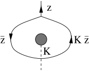
Figure 1: A singlet junction as a loop with an asymptotic string of charge $\bf z$.

Every junction that does not intersect the simple roots can be represented like this, since the roots begin and end on the branes and so lie within the loop, never crossing it. Since the $a_{i}$ vanish, $\bf J$ is a linear combination of $\mbox{\boldmath$\bf\omega$}^{p}$ and $\mbox{\boldmath$\bf\omega$}^{q}$, as in (3.17). Rules for computing the self-intersection of general junctions were discussed in [7]. In this case, the only contribution comes from the point where the asymptotic string joins the loop, and is given in terms of the charges of the string segments by $(\mbox{\boldmath$\bf J$},\mbox{\boldmath$\bf J$})=\mbox{\boldmath$\bf z$}\!\times\!\overline{\mbox{\boldmath$\bf z$}}$, or explicitly

$$(\mbox{\boldmath$\bf J$},\mbox{\boldmath$\bf J$})=\mbox{\boldmath$\bf z$}\times\overline{\mbox{\boldmath$\bf z$}}=-\mbox{\boldmath$\bf z$}^{T}S(K-1\!\!1)^{-1}\mbox{\boldmath$\bf z$}\,,$$ (3.28)

which by (3.18) will be the charge quadratic form $f_{K}({\bf z})$. Defining $t\equiv{\rm Tr\ }K$ and making use of $\hbox{det}\,(K-1\!\!1)=2-t$ and $t{1\!\!1}=K+K^{-1}$, we find:

$$f_{K}({\bf z})\;\;=\;\;\frac{1}{2-t}\,\,{\bf z}^{T}SK\mbox{\boldmath$\bf z$}\;\;\;\equiv\;\;\frac{1}{2-t}\,\,Q_{K}(p,q).$$ (3.29)

Another useful expression for the charge quadratic form which can be derived from (2.4) is

$$f_{K}({\bf z})\;\;=1+\frac{1}{2-t}\{Tr(K_{{\bf z}}K)-2\}.$$ (3.30)

This result indicates that the charge quadratic form $f_{K}({\bf z})$ is determined completely by the $SL(2,{\sf Z\!\!\!Z})$ monodromy matrix of the brane configuration. More explicitly we can write

$$K=\left(\begin{array}[]{cc}a&b\\ c&d\end{array}\right)\;\;\;\to\;\;\;Q_{K}(p,q)=-c\,p^{2}+(a-d)\,p\,q+b\,q^{2}\,.$$ (3.31)

This map from $SL(2,{\sf Z\!\!\!Z})$ to binary quadratic forms is well known in mathematics (see for example [20]). Let us take a moment to explore its properties, as it will turn out to be very useful. The map associates $SL(2,{\sf Z\!\!\!Z})$ matrices of trace $t$ to quadratic forms of discriminant $t^{2}-4$, and turns out to be one-to-one and invertible. The inverse map associates to the quadratic form $Q(p,q)=A\,p^{2}+B\,pq+C\,q^{2}$ the $SL(2,{\sf Z\!\!\!Z})$ matrix of trace $t$ [20]

$$K(Q)=\pmatrix{\frac{t+B}{2}&-C\cr A&\frac{t-B}{2}}\,,$$ (3.32)

with discriminant $B^{2}-4AC=t^{2}-4$, and since $t+B\equiv 0~{}(\mbox{mod}~{}2)$ the entries are integral. This map is natural since the fixed points $x$ of $K$ acting on the upper half plane coincide with the zeroes of $Q_{K}(x,1)$:

$$\frac{ax+b}{cx+d}=x\;\;\;\Longleftrightarrow\;\;\;-cx^{2}+(a-d)x+b=0\,.$$ (3.33)

Moreover, the relation (3.31) establishes a one-to-one correspondence between $SL(2,{\sf Z\!\!\!Z})$ conjugacy classes of trace $t$ and equivalence classes of quadratic forms of discriminant $t^{2}-4$. In other words two $SL(2,{\sf Z\!\!\!Z})$ matrices of trace $t$ are conjugate in $SL(2,{\sf Z\!\!\!Z})$ if and only if the associated quadratic forms are equivalent (i.e. $Q\sim Q^{\prime}$ if $Q^{\prime}(\mbox{\boldmath$\bf z$})=Q(g\mbox{\boldmath$\bf z$})$ for some $g\in SL(2,{\sf Z\!\!\!Z})$). Indeed, we have

$$K^{\prime}=gKg^{-1}\;\;\;\Leftrightarrow\;\;\;Q_{K^{\prime}}({\bf z})=Q_{K}(g^{-1}{\bf z})\,..$$ (3.34)

Let us prove this. By explicit substitution the direction $\Rightarrow$ is straightforward. To see the opposite, consider $K$ and $K^{\prime}$ satisfying $Q_{K^{\prime}}(\mbox{\boldmath$\bf z$})=Q_{K}(g^{-1}\mbox{\boldmath$\bf z$})$ for any $\bf z$:

$$\mbox{\boldmath$\bf z$}^{T}g^{T-1}SKg^{-1}\mbox{\boldmath$\bf z$}=\mbox{\boldmath$\bf z$}^{T}SK\mbox{\boldmath$\bf z$},$$ (3.35)

implying

$$SgKg^{-1}=SK+mS,$$ (3.36)

for some $m$, where we used $Sg=(g^{T})^{-1}S$. Multiplying (3.36) by $S$ and taking the trace of both sides yields $m=0$, proving (3.34). This should not surprise us, since our construction of $f_{K}(p,q)$ was manifestly $SL(2,{\sf Z\!\!\!Z})$-covariant.

We have shown that the monodromy $K$ entirely determines the asymptotic charge form $f(p,q)$, and additionally one can show that from $f(p,q)$ one can uniquely recover $K$. We see that the problem of enumerating the conjugacy classes of $SL(2,{\sf Z\!\!\!Z})$, which in turn determine the possible algebras realized on 7-branes, is equivalent to that of classifying inequivalent quadratic forms. We shall come back to this point later.

3.3 The monodromy and the determinant of $A({\cal G})$

In this section, we shall express the determinant of the Cartan matrix of the semisimple algebra ${\cal G}$ arising on a set of 7-branes in terms of two simple invariants of the 7-brane system, the trace of the monodromy matrix $K$ and the asymptotic charge invariant $\ell$.

For any brane configuration $\mbox{\boldmath$\bf G$}=\mbox{\boldmath$\bf X$}_{1}\mbox{\boldmath$\bf X$}_{2}\ldots\mbox{\boldmath$\bf X$}_{n}$, the metric on the associated lattice of junctions $\Lambda$ is given by [7]

$${\cal A}\equiv\left(\begin{array}[]{cccc}1&a_{12}&\ldots&a_{1n}\\ a_{12}&1&\ldots&a_{2n}\\ \vdots&\vdots&\ddots&\vdots\\ a_{1n}&a_{2n}&\ldots&1\end{array}\right)\hskip 36.135pta_{ij}=-\frac{1}{2}(\mbox{\boldmath$\bf z$}_{i}\times\mbox{\boldmath$\bf z$}_{j})=-\frac{1}{2}(p_{i}q_{j}-q_{i}p_{j}).$$ (3.37)

The volume of the unit cell in the total junction lattice $\Lambda$ is given by $\sqrt{\mbox{det}{\cal A}}$, and one finds that this quantity only depends on the trace of the overall monodromy:

$$\mbox{det}\,{\cal A}=\frac{1}{4}\,\,\hbox{Tr}\,K+\frac{1}{2}\,\,,$$ (3.38)

This equation, which holds for any brane configuration, is proven using (2.9) and (3.37). Since our proof is somewhat technical we have relegated it to the appendix.

The lattice $\Lambda$ has a sublattice $\Lambda_{0}$ containing all junctions with no asymptotic charges. We denote by ${\cal A}_{0}$ the matrix giving the metric on $\Lambda_{0}$ for some specific choice of basis. Being the volume of the unit cell, $\sqrt{\mbox{det}{\cal A}_{0}}$ is basis independent. It is shown in the appendix that

$$\ell^{2}\;\mbox{det}{\cal A}_{0}=2-{\rm Tr\ }K\,.$$ (3.39)

When we have a set of all mutually local branes – for example $\mbox{\boldmath$\bf A$}^{N+1}$ , which realizes ${\cal G}=A_{N}$ – the lattice of asymptotic charges is only one-dimensional, $\ell=0$ and ${\rm Tr\ }K=2$, in which case (3.39) is trivially satisfied. This situation is treated separately in the appendix where we find

$$\mbox{det}{\cal A}_{0}=N+1\,,\qquad\hbox{for}\,\,(N+1)\,\,\hbox{mutually local branes}\,.$$ (3.40)

We now recall that the Lie algebra ${\cal G}$ associated to a brane configuration $\bf G$ is precisely identified by matching the basis basis junctions of $\Lambda_{0}$ to the simple roots of ${\cal G}$ in such a way that inner products coincide [7]. This is exactly the situation when ${\cal G}$ is semisimple, in which case simple roots describe the algebra completely. Then $\mbox{det}{\cal A}_{0}$ coincides with $\mbox{det}A({\cal G})$, the determinant of the Cartan matrix of ${\cal G}$. Indeed, (3.40) is consistent since the $A_{N}$ Cartan matrix has determinant $N+1$. For (3.39) we write

$$\ell^{2}\;\mbox{det}A({\cal G})=2-{\rm Tr\ }K\,.$$ (3.41)

Here, however, we must note that when ${\cal G}$ is not semisimple $A({\cal G})$ is not a Cartan matrix. Consider, for example, the case ${\cal G}=\bar{\cal G}\oplus u(1)$, with $\bar{\cal G}$ semisimple. Assume basis junctions $(\{\mbox{\boldmath$\bf J$}_{i}\},\mbox{\boldmath$\bf J$})$ can be found such that the $\{\mbox{\boldmath$\bf J$}_{i}\}$ generate $\bar{\cal G}$, $\bf J$ carries the $u(1)$ charge, and $\mbox{\boldmath$\bf J$}\cdot\mbox{\boldmath$\bf J$}_{i}=0$. Then $\mbox{det}A({\cal G})=\mbox{det}A(\bar{\cal G})\cdot(-\mbox{\boldmath$\bf J$}^{2})$.

We will use the trace/determinant relation (3.41) in section 7 to fit configurations with various algebras into conjugacy classes of $SL(2,{\sf Z\!\!\!Z})$. For now, let us consider what it tells us about the algebras realized on the configurations ${\bf E_{1}}$ and ${\bf\tilde{E}_{1}}$, which as we mentioned have equivalent $K$ but different $\ell$.

We determined in section 2 that $\ell({\bf E_{1}})=2$. Its monodromy is $K({\bf E_{1}})=\left(-2\;-7\atop-1\;-4\right)$, and consequently, ${\rm Tr\ }K=-6$. Using (3.41), we learn that det$A({\cal G}({\bf E_{1}}))=2$. The only $ADE$ algebra with such a Cartan matrix is ${\cal G}({\bf E_{1}})=A_{1}$. Indeed, explicit examination of the junctions supported on ${\bf E_{1}}$ reveals a single simple root with $\mbox{\boldmath$\bf J$}^{2}=-2$.

The monodromy of ${\bf\tilde{E}_{1}}$ is conjugate to that of ${\bf E_{1}}$, and consequently ${\rm Tr\ }K({\bf\tilde{E}_{1}})=-6$ as well; however, $\ell({\bf\tilde{E}_{1}})=1$. Equation (3.41) then tells us that det$A({\cal G}({\bf\tilde{E}_{1}}))=8$. Thus the algebra cannot be $A_{1}$. However, the configuration has only three branes, and cannot support an algebra with rank greater than one. The only possible conclusion is that $A({\cal G}({\bf\tilde{E}_{1}}))$ is not the Cartan matrix of a semisimple Lie algebra, but instead is just the intersection form of a basis vector corresponding to an Abelian factor. Indeed, the minimal uncharged proper junction on the configuration has self-intersection $\mbox{\boldmath$\bf J$}^{2}=-8$, and so ${\cal G}({\bf\tilde{E}_{1}})=u(1)$.

The 7-brane configurations corresponding to $E_{N}$ can be used to construct ${\cal N}=2$ $D=4$ theories with exceptional global symmetries which are $S^{1}$ compactifications of the five dimensional theories with the same global symmetry [21, 22, 23, 24]. Therefore the presence of two configurations either of which can enhance to $E_{2}$ is consistent with the fact that in five dimensions there are two different theories, $E_{1}$ and $\tilde{E}_{1}$, with $su(2)$ and $u(1)$ global symmetry. These two theories become equivalent to the $E_{2}$ theory after addition of more matter. In [22] these theories were related to shrinking del Pezzo surfaces in a Calabi-Yau threefold. In that framework the two theories $E_{1}$ and $\tilde{E}_{1}$ correspond to the two del Pezzos $\,{\hbox{P}\!\!\!\!\!\hbox{I}\,\,\,}^{1}\times\,{\hbox{P}\!\!\!\!\!\hbox{I}\,\,\,}^{1}$ and ${\cal B}_{1}$, where ${\cal B}_{n}$ is $\,{\hbox{P}\!\!\!\!\!\hbox{I}\,\,\,}^{2}$ blown up at $n$ generic points. It is a known fact that further blowing up either one at a point gives the manifold ${\cal B}_{2}$. Correspondingly, the ${\bf E_{1}}$ and ${\bf{\tilde{E}_{1}}}$ configurations become equivalent as ${\bf E_{2}}$ after addition of a D7-brane.

4 From Kodaira Singularities to Infinite Series

The Kodaira classification of singularities on a K3 manifold tells us that in certain limit of moduli space, a collection of 2-cycles with intersection realizing an $ADE$ Cartan matrix collapse to zero size. In the 7-brane picture, this means that certain sets of 7-branes can be brought to a point. Other configurations, with other possible algebras realized by the intersection form, may not, but are still interesting to study.

In this section we generalize the configurations corresponding to Kodaira singularities into a number of infinite series, recognizing a more systematic way of treating these series in the process. We begin the discussion by examining configurations of two 7-branes, which turn out to be “kernels” for the infinite series we discuss in the second half of the section.

4.1 Classification of configurations of two 7-branes

The complete enumeration of inequivalent configurations of two 7-branes is still a difficult problem, but we shall organize the classification, and examine the first few nontrivial cases.

A pair of 7-branes may be either mutually local or nonlocal. Two mutually local branes are always $SL(2,{\sf Z\!\!\!Z})$-equivalent to $\mbox{\boldmath$\bf A$}_{1}=\mbox{\boldmath$\bf A$}\mbox{\boldmath$\bf A$}$, which realizes the $A_{1}$ algebra and supports only $p$ charge.

Two mutually non-local branes will support junctions with both $p$ and $q$ charge. There are no junctions without asymptotic charge and no enhanced symmetry algebra. If the charges of the 7-branes are $[p,q]$, and $[r,s]$, then $\ell=ps-rq$ from (2.10). Furthermore the trace of the monodromy is readily computed to be

$${\rm Tr\ }K=2-\ell^{2}\,.$$ (4.42)

Note that in larger brane configurations ${\rm Tr\ }K$ need not depend on $\ell$ in any fashion; indeed ${\bf E_{1}}$ and ${\bf\tilde{E}_{1}}$ have identical $K$ despite differing $\ell$. The relationship (4.42) is special to the case of two 7-branes.

We have conjectured that only the equivalence class of $K$, the value of $\ell$ and the number of branes will classify any configuration of 7-branes. In this instance we have fixed the number of branes, and since $\ell$ follows from $K$, we predict that only the equivalence classes of the monodromy will specify equivalence.

Two configurations will only be equivalent if $\ell$ coincides. By separate global $SL(2,{\sf Z\!\!\!Z})$ transformations we can always convert them into the form $\mbox{\boldmath$\bf A$}\mbox{\boldmath$\bf X$}_{\bf[i,\ell]}$, $\mbox{\boldmath$\bf A$}\mbox{\boldmath$\bf X$}_{\bf[j,\ell]}$ where $0\leq i,j\leq~{}\ell$. Configurations with the same $\ell$ may be equivalent if the values $i$, $j$ can be mapped into each other by transformations preserving the form of these configurations.

Since the integers $(i,\ell)$ characterize a 7-brane, we must have gcd$(i,\ell)$=1. In this case there exist integers $(a,b)$ such that $ai-b\ell=1$, using which we can construct an $SL(2,{\sf Z\!\!\!Z})$ matrix:

$$g=\pmatrix{a&-b\cr-\ell&i}.$$ (4.43)

We then apply this transformation, move a branch cut and apply another $SL(2,{\sf Z\!\!\!Z})$ by some power of $K_{A}=\left({1\;-1\atop\!0\;\;\;1}\right)$:

$$\mbox{\boldmath$\bf A$}\mbox{\boldmath$\bf X$}_{\bf[i,\ell]}\stackrel{{\scriptstyle g}}{{\cong}}\mbox{\boldmath$\bf X$}_{\bf[-a,\ell]}\mbox{\boldmath$\bf A$}\,=\mbox{\boldmath$\bf A$}\mbox{\boldmath$\bf X$}_{\bf[-a-\ell,\ell]}\stackrel{{\scriptstyle(K_{A})^{n}}}{{\cong}}\mbox{\boldmath$\bf A$}\mbox{\boldmath$\bf X$}_{\bf[a^{*},\ell]}\,,$$ (4.44)

where in the power $n$ of $K_{A}$ is chosen to as to obtain

$$0\leq a^{*}\leq\ell\,,\qquad\hbox{with}\quad a^{*}=-a\quad(\hbox{mod}\,\ell)\,.$$ (4.45)

This result helps the classification as follows. For a given $\ell$ the above relation will provide equivalences between $\mbox{\boldmath$\bf A$}\mbox{\boldmath$\bf X$}_{\bf[i,\ell]}$ configurations with different allowed values of $i$. Configurations that cannot be made equivalent in this way, may or may not be equivalent. Let us now catalog the first few cases.

The value ${\rm Tr\ }K=+2$ corresponds the two 7-branes being are mutually local. The brane configuration is then always equivalent to an ${\bf AA}$ configuration and the resulting gauge algebra is $A_{1}$. As an aside, since affine algebras can only arise for ${\rm Tr\ }K=+2$ (see [11, 12]) this implies that affine algebras cannot arise with just two 7-branes.

The case $\ell=1$ gives ${\rm Tr\ }K=1$ and can be achieved with $\mbox{\boldmath$\bf A$}\mbox{\boldmath$\bf X$}_{\bf[i,{\bf 1}]}$. Here the two possible cases $i=0$ and $i=1$ are manifestly equivalent by suitable $K_{A}$ conjugation. We find it convenient to choose the representative ${\bf H_{0}}=\mbox{\boldmath$\bf X$}_{\bf[0,-1]}{\bf C}$, the first element of the Argyres-Douglas series, and a Kodaira configuration in its own right. We can show it is equivalent to the canonical form by $\mbox{\boldmath$\bf X$}_{\bf[0,-1]}{\bf C}=\mbox{\boldmath$\bf A$}\mbox{\boldmath$\bf X$}_{\bf[0,-1]}=\mbox{\boldmath$\bf A$}\mbox{\boldmath$\bf X$}_{\bf[0,1]}$.

For $\ell=2$, ${\rm Tr\ }K=-2$ and the unique realization is $\mbox{\boldmath$\bf A$}\mbox{\boldmath$\bf X$}_{\bf[1,2]}$ since $i=0,2$ do not denote good 7-branes. We can represent this case by the ${\bf D_{0}}={\bf BC}$ system, as global action of $g=\left({1\;0\atop 1\;1}\right)$ on ${\bf BC}$ gives us $\mbox{\boldmath$\bf A$}\mbox{\boldmath$\bf X$}_{\bf[1,2]}$. ${\bf D_{0}}$ is the background 7-brane configuration for realizing the familiar $SU(2)$ Seiberg-Witten theory with $N_{f}=0$ on the world volume of a D3-brane probe.

The case $\ell=3$ giving ${\rm Tr\ }K=-7$ can be realized as $\mbox{\boldmath$\bf A$}\mbox{\boldmath$\bf X$}_{\bf[1,3]}$ and as $\mbox{\boldmath$\bf A$}\mbox{\boldmath$\bf X$}_{\bf[2,3]}$. It is simple to verify using (4.44), (4.45) that these two are actually equivalent. We can therefore choose to represent this case by ${\bf E_{0}}={\bf X_{\bf[2,-1]}C}$, a configuration with $\ell=3$. This will be the kernel for the exceptional series.

We do not find two inequivalent configurations until $\ell=5$, where ${\rm Tr\ }K=-23$. The brane configurations are $\mbox{\boldmath$\bf A$}\mbox{\boldmath$\bf X$}_{\bf[1,5]}\cong\mbox{\boldmath$\bf A$}\mbox{\boldmath$\bf X$}_{\bf[4,5]}$ and $\mbox{\boldmath$\bf A$}\mbox{\boldmath$\bf X$}_{\bf[2,5]}\cong\mbox{\boldmath$\bf A$}\mbox{\boldmath$\bf X$}_{\bf[3,5]}$. Inequivalence is proved explicitly by a calculation showing that the monodromies are not conjugate in $SL(2,{\sf Z\!\!\!Z})$.

One can continue in this fashion without encountering much new. Let us now turn to the infinite series we can generate from these two 7-brane kernels.

4.2 Infinite Series

The examples of $A_{N}$, $D_{N}$ and $E_{N}$ Kodaira singularities [25] have been studied considerably, and have been associated with the 7-brane configurations [26]:

$${\bf A}_{\bf N} : {\bf AA\ldots A}\equiv{\bf A}^{N+1}$$

$${\bf D}_{\bf N\geq 4} : {\bf A}^{N}{\bf BC}$$ (4.46)

$${\bf E}_{\bf 6},{\bf E}_{\bf 7},{\bf E}_{\bf 8} : {\bf A}^{5}{\bf BCC},{\bf A}^{6}{\bf BCC},{\bf A}^{7}{\bf BCC}$$

$${\bf H}_{\bf 0},{\bf H}_{\bf 1},{\bf H}_{\bf 2} : {\bf AC},{\bf AAC},{\bf AAAC}.$$

The ${\bf D}_{\bf 4},{\bf E}_{\bf 6},{\bf E}_{\bf 7},{\bf E}_{\bf 8}$ correspond to orbifold singularities of the K3, and the ${\bf H}_{\bf 0},{\bf H}_{\bf 1},{\bf H}_{\bf 2}$ are the Argyres-Douglas points with associated algebras ${\cal G}=0,A_{1},A_{2}$. These configurations are “dual” to the ${\bf E_{N}}$ in the sense that ${\bf E_{N}}$ and ${\bf H_{8-N}}$ can be realized with the same constant value of $\tau$ and together the net monodromy is unity.

These configurations naturally suggest generalizations. The non-collapsible ${\bf D_{N}}$ configurations with $N=3,2,1,0$ support algebras $D_{3}=A_{3}$, $D_{2}=A_{1}\oplus A_{1}$, $D_{1}=u(1)$ and $D_{0}=0$, and are backgrounds of a probe D3-brane realization for the Seiberg-Witten theories with $N$ flavors, where the 7-brane algebra is realized as a global symmetry.

Similarly, we can extend ${\bf E_{N}}$ to ${\bf A}^{N}{\bf BCC}$ with $N=1,2,3,4,5$, realizing the algebras $E_{1}=A_{1}$, $E_{2}=A_{1}\oplus u(1)$, $E_{3}=A_{2}\oplus A_{1}$, $E_{4}=A_{4}$, and $E_{5}=D_{5}$. We have already seen that ${\bf E_{5}}\cong{\bf D_{5}}$, and one can also confirm ${\bf E_{4}}\cong{\bf H_{4}}$. Continuing the ${\bf E_{N}}$ series beyond $N=8$ one encounters ${\bf E_{9}}$ which gives rise to the affine algebra $E_{9}=\widehat{E}_{8}$ [11], which we shall have more to say about in the sequel paper [12].

The $SL(2,{\sf Z\!\!\!Z})$ equivalence transformations are also useful in unifying the description of the ${\bf D}$, ${\bf E}$, ${\bf H}$ series which gives hint to further generalization. It is straightforward to check the following identity:

$${\bf A}^{N+1}{\bf C}\stackrel{{\scriptstyle K_{A}}}{{\cong}}{\bf A}^{N+1}{\bf X_{\bf[0,-1]}}={\bf A}^{N}{\bf X_{\bf[0,-1]}C}\,,$$ (4.47)

which allows us alternately to describe this series as ${\bf\tilde{H}_{N}}={\bf A}^{N}{\bf X_{[0,-1]}C}\,$. Thus the kernel ${\bf H_{0}}$ from the previous section generates the entire Argyres-Douglas series just by adding $\bf A$-branes.

Similarly, the ${\bf D_{N}}$ series is described by ${\bf D_{N}}={\bf A}^{N}{\bf X_{[1,-1]}C}\,,$ where we have written explicitly the charges of the $\bf B$-brane. It is generated from the ${\bf D_{0}}$ kernel. Notice that although $\ell({\bf D_{0}})=2$, $\ell({\bf D_{N}})=1$ for $N>0$.

This now suggests a similar possibility for the ${\bf E_{N}}$ series. Indeed, we noted in (2.14) that

$${\bf A}^{N-1}{\bf BCC} \cong {\bf A}^{N}{\bf X_{[2,-1]}C},$$ (4.48)

where the conjugation is with the matrix $K_{A}$. This enables us to write another presentation for the $E_{N}$ series as ${\bf\tilde{E}_{N}}={\bf A}^{N}{\bf X_{[2,-1]}C}\,$. We see that the ${\bf E_{0}}$ kernel does indeed generate the entire series. As we discussed in section 2, the ${\bf E_{N}}$ and ${\bf\tilde{E}_{N}}$ series are only equivalent for $N\geq 2$, while ${\bf E_{1}}$ and ${\bf\tilde{E}_{1}}$ are not equivalent.

With these examples in mind, we recognize the significance of the Kodaira series. ${\bf A_{N}}$ may be thought of as the series that results from adding a number of $\bf A$-branes to a kernel of a single $\bf A$-brane. Similarly, ${\bf H_{N}}$, ${\bf D_{N}}$ and ${\bf E_{N}}$ are the three simplest series generated from kernels of two branes.

The three series of configurations can be uniformly described as:

$${\bf S_{p,N}}={\bf A}^{N}{\bf X_{[p,-1]}C}\,,$$ (4.49)

with $p=0,1,2$ for the ${\bf\tilde{H}_{N}},{\bf D_{N}}$ and ${\bf\tilde{E}_{N}}$ series, respectively. Notice that in all cases, $\ell=1$ for $N\geq 1$.

To see how the Lie algebras arise, we show in Fig. 2 the simple root junctions whose intersection form produces the corresponding Cartan matrix. The trace of the overall monodromy is

$${\rm Tr\ }K({\bf S_{p,N}})=2-(p+1)^{2}+(p-1)N\,,$$ (4.50)

so that $2-{\rm Tr\ }K(p,N)=(p+1)^{2}-(p-1)N$ which reproduces the expected relation to the determinant of the Cartan matrices: det$\,(A(A_{N}))=N+1$, det$\,(A(D_{N}))=4$ and det$\,(A(E_{N}))=9-N$.

Figure 2: (a) Brane configuration of the ${\bf H}$, ${\bf D}$, ${\bf E}$ and the generalized ${\bf S_{p}}$ series. (b) Dynkin diagrams of the algebras $A_{N}$, $D_{N}$, $E_{N}$ and $T_{p+1,2,N-1-p}$.

Notice that besides the series of finite $A$ and $D$ algebras, we have constructed $E_{N}$ whose elements are infinite dimensional Kac-Moody algebras for $N>8$. In fact one could go further by engineering new algebra realizations with $p>2$, those Dynkin diagrams are shown in Fig. 2(b) and are usually denoted as $T_{p+1,2,n-1-p}$. Finally the simple root junctions suggest how to the realize ${\cal G}=T_{r_{1},r_{2},r_{3}}$: the configuration is ${\bf A}^{r_{1}+r_{2}}{\bf X_{[r_{1}-1,-1]}}{\bf C}^{r_{2}-1}$, the simple roots are shown in Fig. 3(a), and one can check that (3.41) is satisfied. We shall not pursue these exotic series further; no doubt there is more to be said. We shall have more to say about infinite-dimensional algebras in [12].

Figure 3: (a) Brane configuration of ${\cal G}=T_{r_{1},r_{2},r_{3}}$. (b) Dynkin diagram of ${\cal G}=T_{r_{1},r_{2},r_{3}}$.

It is remarkable that we have found two series, ${\bf A_{N}}$ and ${\bf H_{N}}$, realizing the $A_{N}$ algebras, the former supporting junctions with only $p$ charge and $\ell=0$, the latter with both $p$ and $q$ asymptotic charges and $\ell=1$. In fact there are an infinite number of such series, parameterized by $\ell$.

Take any kernel of two 7-branes with some value $\ell$, and perform an $SL(2,{\sf Z\!\!\!Z})$ transformation such that one of the 7-branes is an $\bf A$-brane, ${\bf\mbox{\boldmath$\bf A$}\mbox{\boldmath$\bf X$}_{[i,\ell]}}$, as in the previous subsection. One may add additional $\bf A$-branes without modifying $\ell$, to obtain a series

$${\bf A^{{\bf i}\,\ell}_{N}}\equiv\mbox{\boldmath$\bf A$}^{N+1}\mbox{\boldmath$\bf X$}_{\bf[i,\ell]}\,,$$ (4.51)

which has ${\cal G}=A_{N}$ and asymptotic charge invariant $\ell$. Configurations with different $\ell$ are obviously inequivalent, thus proving there are an infinite number of series realizing $A_{N}$. We have not found any analogous configurations for the $D_{N}$ and $E_{N}$ algebras, which seem to appear on just one series each.

Notice that, like the ${\bf S_{p,N}}$ series, the ${\bf A_{N}^{{\bf i}\,\ell}}$ series arise from adding $\bf A$-branes to a kernel of two 7-branes with some $\ell$. They differ in the $SL(2,{\sf Z\!\!\!Z})$ presentation of that kernel, relative to the $\bf A$-branes.

We shall end our discussion of series of 7-branes here, since we have found more than enough to occupy our attention. This technique of beginning with a known configuration and enhancing it by adding a new brane is a powerful one, and offers insight into how the monodromy fixes the algebra by means of the quadratic form. We shall explore it systematically in the next section.

$\mathcal{G}$	Brane Configuration	$K$	$f_{K}(p,q)$
$A_{N}$	${\bf{A}_{N}}={\bf A}^{N+1}$	$\pmatrix{1&-N-1\cr 0&1}$	$-\frac{1}{N+1}p^{2}$
	${\bf{H}_{N}}={\bf A}^{N+1}{\bf C}$	$\pmatrix{2&-3-2N\cr 1&-N-1}$	$\frac{1}{N+1}\{-p^{2}+(N+3)pq-(3+2N)q^{2}\}$
	$\rule{0.0pt}{19.91692pt}{\bf\tilde{H}_{N}}={\bf A}^{N}{\bf X}_{\bf[0,-1]}{\bf C}$	$\pmatrix{1&-N-1\cr 1&-N}$	$\frac{1}{N+1}\{-p^{2}+(N+1)pq-(N+1)q^{2}\}$
$D_{N}$	${\bf D_{N}}={\bf A}^{N}{\bf BC}$	$\pmatrix{-1&N-4\cr 0&-1}$	$\frac{N-4}{4}q^{2}$
$E_{N}$	${\bf E_{N}}={\bf A}^{N-1}{\bf BCC}~{}$	$\pmatrix{-2&2N-9\cr-1&N-5}$	$\frac{1}{9-N}\{p^{2}+(3-N)pq+(2N-9)q^{2}\}$
	${\bf\tilde{E}_{N}}={\bf A}^{N}{\bf X}_{\bf[2,-1]}{\bf C}$	$\pmatrix{-3&3N-11\cr-1&N-4}$	$\frac{1}{9-N}\{p^{2}+(1-N)pq+(3N-11)q^{2}\}$

Table 1: Brane configurations, monodromies and the charge quadratic form for $A_{N},D_{N}$ and $E_{N}$ algebras. The two series (${\bf H_{N}}$ and ${\bf\tilde{H}_{N}}$) realizing the $A_{N}$ algebras are equivalent. The two series (${\bf E_{N}}$ and ${\bf\tilde{E}_{N}}$) realizing $E_{N}$ are equivalent for $N\geq 2$.

5 Transitions Between 7-Brane Configurations

We have examined several series of finite Lie algebras arising on 7-branes. Keeping in mind the general question of understanding all possible configurations, in the present section we address transitions from one algebra to another. Here we shall see how the charge quadratic form $f(p,q)$ controls the change from one algebra to the other. Suppose we have a brane configuration $\bf G$ with monodromy $K$ and quadratic form $f_{K}$ that realizes a finite Lie algebra ${\cal G}$. When we add one more 7-brane $\bf Z$ with charge $\mbox{\boldmath$\bf z$}=[p,q]$, we obtain a new configuration ${\bf G}^{enh}=\mbox{\boldmath$\bf G$}\mbox{\boldmath$\bf Z$}$, where we have conventionally placed the new brane on the right of the configuration (see Fig. 4). Additional junctions with support on the new brane appear, resulting in an enhancement from ${\cal G}$ to some larger algebra ${\cal G}^{enh}$.

Which algebra ${\cal G}^{enh}$ is obtained depends on ${\cal G}$ and on the charge $\bf z$ of $\bf Z$. Recall that $f(\mbox{\boldmath$\bf z$})=f(\mbox{\boldmath$\bf z$}^{\prime})$ when $\mbox{\boldmath$\bf z$}^{\prime}=g\mbox{\boldmath$\bf z$}$ with $g\in SL(2,{\sf Z\!\!\!Z})$ and $gKg^{-1}=K$. As a result, the total monodromy $K_{\mbox{\boldmath$\bf z$}}\,K$ of ${\bf G}^{enh}$ is conjugate to $K_{\mbox{\boldmath$\bf z$}^{\prime}}\,K$, and we expect both $\bf Z$ and $\mbox{\boldmath$\bf Z$}^{\prime}$ to enhance ${\cal G}$ to the same ${\cal G}^{enh}$. The enhancing 7-branes can therefore be grouped into classes; all elements of a given class give the same enhancement. The charge quadratic form $f(\mbox{\boldmath$\bf z$})$ thus measures how the monodromy “sees” the charges of the enhancing brane. In general $\mbox{rank}({\cal G}^{enh})=\mbox{rank}({\cal G})+1$ (except when the initial configuration contains only mutually local branes, in which case adding a mutually nonlocal brane will not enhance ${\cal G}$) and so the enhancing brane opens up a new direction in the weight lattice.

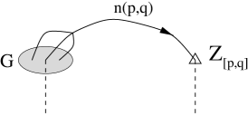
Figure 4: The enhanced configuration ${\bf G}^{enh}$ is obtained by adding a ${\bf Z_{[p,q]}}$-brane to the original configuration $\bf G$. A generic junction has support on the new brane.

To investigate the enlarged root lattice, we construct all junctions on ${\bf G}^{enh}$ having zero total asymptotic charge. Each can be written

$$\mbox{\boldmath$\bf J$}=-n\ \mbox{\boldmath$\bf z$}+n\,(p\,\mbox{\boldmath$\bf\omega$}^{p}+q\,\mbox{\boldmath$\bf\omega$}^{q})+\sum_{i}a_{i}\,\mbox{\boldmath$\bf\omega$}^{i}\,,$$ (5.52)

where the $\mbox{\boldmath$\bf\omega$}^{i}$ are the weight junctions for ${\cal G}$ and have zero asymptotic charge, and $\{\mbox{\boldmath$\bf\omega$}^{p},\mbox{\boldmath$\bf\omega$}^{q}\}$ are the singlets of ${\cal G}$ with asymptotic charges $\mbox{\boldmath$\bf z$}_{p}=(1,0)$ and $\mbox{\boldmath$\bf z$}_{q}=(0,1)$. This junction can be visualized as a sub-junction which leaves the $\bf G$ configuration with charges $(np,nq)$ and ends on the $\bf Z$ brane, where it has $n$ prongs, as in Fig. 4. The self-intersection of $\bf J$ is readily calculated, since there are no cross-terms between the $\bf G$ sub-junction and the $\bf Z$-brane prongs. We find

$$\mbox{\boldmath$\bf J$}^{2}=-n^{2}+n^{2}f(\mbox{\boldmath$\bf z$})-\lambda\cdot\lambda\,,$$ (5.53)

where $\mbox{\boldmath$\bf J$}^{2}=(\mbox{\boldmath$\bf J$},\mbox{\boldmath$\bf J$})$, and $\lambda=\sum_{i}\,a_{i}\,\omega^{i}$ is the ${\cal G}$ weight vector. A minor rearrangement gives

$$\lambda\cdot\lambda=-\mbox{\boldmath$\bf J$}^{2}+n^{2}(f(\mbox{\boldmath$\bf z$})-1)\,.$$ (5.54)

New junctions appear whenever this equation has a solution with non-vanishing grade $n$, and we identify them as the roots of the algebra ${\cal G}^{enh}$. For each value of $\lambda\cdot\lambda$ there are a number of weight vectors $\lambda$, filling out a Weyl orbit of ${\cal G}$, and there will be a distinct root of ${\cal G}^{enh}$ for each distinct weight $\lambda$. Thus each ${\cal G}$ root junction can be characterized by $\mbox{\boldmath$\bf\alpha$}=(n,\lambda)$. Since $\lambda\cdot\lambda\geq 0$ always and supersymmetry requires $\mbox{\boldmath$\bf J$}^{2}\geq-2$, it is possible that (5.54) cannot be satisfied for some $n$, in which case there are simply no root junctions at that $n$. Naturally the roots of ${\cal G}$ appear as $(0,\alpha_{{\cal G}})$.

Since roots have no overall asymptotic charge, it is natural to interpret equation (5.53) as $\mbox{\boldmath$\bf J$}^{2}=-\Lambda\cdot\Lambda$, where $\Lambda$ is a ${\cal G}^{enh}$ weight vector. The length squared of the ${\cal G}^{enh}$ weight vector is given in terms of the length squared of the ${\cal G}$ weight vector plus a contribution along the new axis in the weight lattice, with $(1-f(\mbox{\boldmath$\bf z$}))$ setting the scale for the new direction.

Once we have determined the root system of ${\cal G}^{enh}$, we next find a subset of simple roots. This requires ensuring that any root can be written in the basis of simple roots with coefficients that are either all positive or all negative integers. The simple roots then determine both the Cartan matrix and the Dynkin diagram of ${\cal G}^{enh}$. Simple roots of Kac-Moody Lie algebras are always real, meaning the corresponding junctions have $\mbox{\boldmath$\bf J$}^{2}=-2$.

Since the rank increases by one, generically we need exactly one new root in addition to the simple roots of ${\cal G}$ to complete the set of simple roots for ${\cal G}^{enh}$. (A few exotic cases where two (linearly dependent) new simple roots are necessary are examined in [12]; in all these cases ${\cal G}^{enh}$ is an infinite-dimensional algebra.)

When there is a single new simple root $\mbox{\boldmath$\bf\alpha$}_{0}=(n_{0},\lambda_{0})$, it must be that $|n_{0}|\leq|n|$ for any $n$ with solutions for (5.54) since we need to write any root as an integer linear combination of simple roots, and all other simple roots have $n=0$. Let $W_{0}$ denote the Weyl orbit at grade $n_{0}$. Each root $\mbox{\boldmath$\bf\alpha$}=(n_{0},\lambda)$ which is associated to a weight $\lambda\in W_{0}$ must be positive, since ${\mbox{\boldmath$\bf\alpha$}}=\ldots+{\mbox{\boldmath$\bf\alpha$}_{0}}$ (i.e. the coefficient of $\mbox{\boldmath$\bf\alpha$}_{0}$ is already positive). It is then necessary that $\lambda-\lambda_{0}$ be a positive root of ${\cal G}$ for every $\lambda\in W_{0}$. This implies that $\lambda_{0}$ must be the lowest weight $\theta_{<}$ in the Weyl orbit $W_{0}$.

In the next section we shall explore how the value $f(\mbox{\boldmath$\bf z$})$ determines the type of enhancement that occurs. We shall consider only enhancements to finite ${\cal G}^{enh}$. Enhancements to infinite-dimensional ${\cal G}^{enh}$ are examined in [12]. The structure that we shall find is summarized in Table 2.

$\rule{0.0pt}{14.22636pt}f(\mbox{\boldmath$\bf z$})$	${\cal G}^{enh}$
$f(\mbox{\boldmath$\bf z$})<-1$	${\cal G}\oplus u(1)$
$f(\mbox{\boldmath$\bf z$})=-1$	${\cal G}\oplus A_{1}$
$-1<f(\mbox{\boldmath$\bf z$})<1$	finite
$f(\mbox{\boldmath$\bf z$})=1$	affine
$f(\mbox{\boldmath$\bf z$})>1$	indefinite

Table 2: Algebraic enhancements of brane configurations. Adding one brane to an existing configuration, the asymptotic charge form $f(\mbox{\boldmath$\bf z$})$ of ${\bf G}$ evaluated on the new brane determines the type of ${\cal G}^{enh}$.

6 Finite Enhancement: $f(\mbox{\boldmath$\bf z$})<1$

Let us explore how the value of $f(\mbox{\boldmath$\bf z$})$ determines the enhanced algebra. First, consider the values $f(\mbox{\boldmath$\bf z$})<-1$; it is easy to see that equation (5.54) cannot be satisfied simultaneously with $\mbox{\boldmath$\bf J$}^{2}\geq-2$. Thus no new roots will appear, and we merely find ${\cal G}^{enh}={\cal G}\oplus u(1)$.

At the saturating value $f(\mbox{\boldmath$\bf z$})=-1$,

$$\lambda\cdot\lambda=-\mbox{\boldmath$\bf J$}^{2}-2n^{2}\,,$$ (6.55)

which only has solutions for $\mbox{\boldmath$\bf J$}^{2}=-2$, with $\lambda\cdot\lambda=0$ and $n=\pm 1$. The new simple root is $\mbox{\boldmath$\bf\alpha$}_{0}=(n_{0},\lambda)=(1,0)$, and satisfies $(\mbox{\boldmath$\bf\alpha$}_{0},\mbox{\boldmath$\bf\alpha$}_{i})=0$ for all $\mbox{\boldmath$\bf\alpha$}_{i}$ in ${\cal G}$. Thus the enhancement is ${\cal G}^{enh}={\cal G}\oplus A_{1}$, independent of ${\cal G}$.

Now consider the range $-1<f(\mbox{\boldmath$\bf z$})<1$, or equivalently, where the coefficient $(f(\mbox{\boldmath$\bf z$})-1)$ of $n^{2}$ in (5.54) is negative. It follows that this equation only has solutions for $\mbox{\boldmath$\bf J$}^{2}=-2$, all of which are roots of ${\cal G}^{enh}$ with $\Lambda\cdot\Lambda=2$. Moreover the number of new roots is finite, for (5.54) will have no solution for sufficiently large $|n|$. Therefore ${\cal G}^{enh}$ is a finite Lie algebra. We

now give several examples of this case.

Consider the ${\bf H_{N}}$ series, representing the algebra $A_{N}$ on branes $\mbox{\boldmath$\bf A$}^{N+1}\mbox{\boldmath$\bf C$}$. The $\bf C$-brane enables the configuration of otherwise mutually local branes to have junctions with asymptotic $q$-charge , thus making it possible for new roots to stretch to an enhancing $[p,q]$ brane when it is added. The charge quadratic form is (see table 1)

$$f(p,q)=-\,\frac{1}{N+1}\;(p^{2}-(N+3)pq+(2N+3)q^{2})\,,$$ (6.56)

and will determine what kind of enhanced algebra appears.

The simplest enhancement occurs when the new brane is another $[1,0]$, $f(1,0)=-1/(N\!+\!1)$. The only junctions satisfying (5.54) besides the roots of $A_{N}$ have $|n|=1$ and $\lambda\cdot\lambda=N/(N\!+1\!)$, requiring either $\lambda\in{\bf N+1}$ (fundamental) or $\lambda\in{\bf\overline{N+1}}$ (antifundamental). We can choose $\mbox{\boldmath$\bf\alpha$}_{0}=(1,\lambda)$ with $\lambda=-\omega^{1}$ or $\lambda=-\omega^{N}$. In either case we get a total of $2(N+1)$ new roots from $n=\pm 1$, the number of roots needed to enhance from $A_{N}$ to $A_{N+1}$. Indeed, $(\mbox{\boldmath$\bf\alpha$}_{0},\mbox{\boldmath$\bf\alpha$}_{i})=-(\mbox{\boldmath$\bf\omega$}^{1},\mbox{\boldmath$\bf\alpha$}_{i})=\delta^{1}_{i}$ or $(\mbox{\boldmath$\bf\alpha$}_{0},\mbox{\boldmath$\bf\alpha$}_{i})=-(\mbox{\boldmath$\bf\omega$}^{N},\mbox{\boldmath$\bf\alpha$}_{i})=\delta^{N}_{i}$, and either choice reproduces the Cartan matrix and Dynkin diagram of $A_{N+1}$. As expected, we enhance to ${\bf H_{N+1}}$.

$\rule{0.0pt}{14.22636pt}{\cal G}$	Config	Branes	$f(\mbox{\boldmath$\bf z$})$	${\cal G}^{enh}$	Enh. branes
			$-1/N$	$A_{N+1}$	$\mbox{\boldmath$\bf A$}{\bf H_{N}}$
$A_{N}$	${\bf H_{N}}$	$\mbox{\boldmath$\bf A$}^{N+1}\mbox{\boldmath$\bf C$}$	$(N\hskip-2.0pt-\hskip-2.0pt3)/(N\hskip-2.0pt+\hskip-2.0pt1)$	$D_{N+1}$	${\bf H_{N}}\mbox{\boldmath$\bf X$}_{\bf[3,1]}$
			$(2N\hskip-2.0pt-\hskip-2.0pt7)/(N\hskip-2.0pt+\hskip-2.0pt1)$	$E_{N+1}$	${\bf H_{N}}\mbox{\boldmath$\bf X$}_{\bf[4,1]}$
$D_{N}$	${\bf D_{N}}$	$\mbox{\boldmath$\bf A$}^{N}\mbox{\boldmath$\bf B$}\mbox{\boldmath$\bf C$}$	$0$	$D_{N+1}$	$\mbox{\boldmath$\bf A$}{\bf D_{N}}$
			$(N-4)/4$	$E_{N+1}$	${\bf D_{N}}\mbox{\boldmath$\bf C$}$
$A_{1}$	${\bf E_{1}}$	$\bf B$$\bf C$$\bf C$	$a^{2}/2-1$	$\tilde{A_{2}}^{(a)}$	${\bf E_{1}}\mbox{\boldmath$\bf X$}_{\bf[2a-1,1]}$
$\rule{0.0pt}{14.22636pt}D_{4}$	${\bf D_{4}}$	${\bf A}^{4}{\bf BC}$	$0$	$D_{5}$	${\bf D_{4}}\mbox{\boldmath$\bf X$}_{\bf[p,q]}$
			$0$	$D_{6}$	$\mbox{\boldmath$\bf A$}{\bf D_{5}}$
$D_{5}$	${\bf D_{5}}$	$\mbox{\boldmath$\bf A$}^{5}\mbox{\boldmath$\bf B$}\mbox{\boldmath$\bf C$}$	$1/4$	$E_{6}$	${\bf D_{5}}\mbox{\boldmath$\bf C$}$
	$\cong{\bf E_{5}}$		$1$	$\widehat{D}_{5}$	${\bf D_{5}}\mbox{\boldmath$\bf X$}_{\bf[1,2]}$
			$9/4$	$E_{4}^{H}$	${\bf D_{5}}\mbox{\boldmath$\bf X$}_{\bf[1,3]}$
			$1/3$	$E_{7}$	$\mbox{\boldmath$\bf A$}{\bf E_{6}}$
$E_{6}$	${\bf E_{6}}$	$\mbox{\boldmath$\bf A$}^{5}\mbox{\boldmath$\bf B$}\mbox{\boldmath$\bf C$}\mbox{\boldmath$\bf C$}$	$1$	$\widehat{E}_{6}$	${\bf E_{6}}\mbox{\boldmath$\bf X$}_{\bf[3,1]}$
			$7/3$	$E_{5}^{H}$	${\bf E_{6}}\mbox{\boldmath$\bf X$}_{\bf[4,1]}$
			$1/2$	$E_{8}$	$\mbox{\boldmath$\bf A$}{\bf E_{7}}$
$E_{7}$	${\bf E_{7}}$	$\mbox{\boldmath$\bf A$}^{6}\mbox{\boldmath$\bf B$}\mbox{\boldmath$\bf C$}\mbox{\boldmath$\bf C$}$	$1$	$\widehat{E}_{7}$	${\bf E_{7}}\mbox{\boldmath$\bf X$}_{\bf[3,1]}$
			$5/2$	$E_{6}^{H}$	${\bf E_{7}}\mbox{\boldmath$\bf X$}_{\bf[4,1]}$
$E_{8}$	${\bf E_{8}}$	$\mbox{\boldmath$\bf A$}^{7}\mbox{\boldmath$\bf B$}\mbox{\boldmath$\bf C$}\mbox{\boldmath$\bf C$}$	$1$	$\widehat{E}_{8}=E_{9}$	$\mbox{\boldmath$\bf A$}{\bf E_{8}}$
			$3$	$E_{7}^{H}$	${\bf E_{8}}\mbox{\boldmath$\bf X$}_{\bf[4,1]}$

Table 3: Finite algebras ${\cal G}$ and enhanced algebras ${\cal G}^{enh}$ obtained by adding a single $\mbox{\boldmath$\bf z$}=[p,q]$ brane. The Dynkin diagram of $\tilde{A}_{2}^{(a)}$ has two nodes with $a$ lines joining them.

Another possibility that proceeds identically for any algebra in the series is to add another $[1,1]$ brane. We would expect that the pair of $\bf C$-branes will now form an additional $A_{1}$ algebra, giving $A_{N}\oplus A_{1}$. Indeed, as $f(1,1)=-1$ for all $N$, and, as mentioned above, this simply adds an additional $A_{1}$ algebra.

Other enhancements are possible. For example, adding a $[3,1]$-brane gives $f(3,1)\!\!=\!\!(N\!-\!3)\,/\,(N\!+\!1)$, so at $n^{2}=1$, $\lambda\cdot\lambda=2(N-1)/(N+1)$. This is the Weyl orbit with dominant weight $\omega^{2}$ (or conjugate) and thus the new simple root is $\mbox{\boldmath$\bf\alpha$}_{0}=(1,-\omega^{2})$. The inner products of this with the other simple roots show the enhancement $A_{N}\rightarrow D_{N+1}$. We can pass the $[3,1]$-brane through the $[1,1]$ branch cut to turn it into a $[1,-1]$-brane, thus recovering the canonical form of the ${\bf D_{N}}$ series. Analogously, adding a $[4,1]$-brane enhances to the $E_{N}$ series. In general a $[p,1]$-brane adds a node connecting to the $(p-1)^{th}$ node of the $A_{N}$ Dynkin diagram.

Naturally we do not need to begin with the ${\bf H_{N}}$ series. One can consider enhancing the ${\bf D_{N}}$ or ${\bf E_{N}}$ series as well. A particularly interesting example is $D_{4}$, on $\mbox{\boldmath$\bf A$}^{4}\mbox{\boldmath$\bf B$}\mbox{\boldmath$\bf C$}$. For this

case $f(p,q)$ vanishes identically, and thus the enhanced algebra ${\cal G}^{enh}$ is independent of the charges $\mbox{\boldmath$\bf z$}=[p,q]$ of the enhancing brane $\bf Z$. This is easy to understand: the monodromy of $D_{4}$ is minus the identity matrix and is invariant under the $SL(2,{\sf Z\!\!\!Z})$ transformation relating any two choices for new branes. We have $\mbox{\boldmath$\bf\alpha$}_{0}=(1,\lambda)$ with $\lambda\cdot\lambda=1$, and therefore $\mbox{\boldmath$\bf\alpha$}_{0}=(1,-\omega^{i})$ where $\omega^{i}=1,3,4$ is the highest weight of the ${\bf 8_{v}}$, ${\bf 8_{s}}$ or ${\bf 8_{c}}$ representation. For any of these three choices, the enhanced algebra is ${\cal G}^{enh}=D_{5}$, a manifestation of triality.

The various $D_{N}$ algebras can enhance to $E_{N+1}$ algebras. For $D_{N}$, $f(p,q)=(N-4)\,q^{2}/4$, and the value of $p$ does not affect the resulting enhancement. As an example, $q=1$ gives $f(\mbox{\boldmath$\bf z$})=(N-4)/4$, which means the new roots $(1,\lambda)$ have $\lambda\cdot\lambda=n/4$. Such weights belong to the spinor representations and enhancement proceeds by attaching a new node to a node associated to a spinor representation, the result being $E_{N+1}$. If $p=1$, $E_{N+1}$ is obtained in the canonical form; otherwise a global $SL(2,{\sf Z\!\!\!Z})$ transformation is necessary to recover the usual monodromy.

If we restrict ourselves to $f(\mbox{\boldmath$\bf z$})<1$ it is simple to show that $E_{6}$ can only enhance to $E_{7}$, that $E_{7}$ can only enhance to $E_{8}$ and that $E_{8}$ cannot enhance to any finite algebra. This last fact follows simply because for $E_{8}$ one has $f(\mbox{\boldmath$\bf z$})\geq 1$ for any choice of $\mbox{\boldmath$\bf z$}\not=0$.

As $N$ increases in the ${\bf H_{N}}$, ${\bf D_{N}}$ and ${\bf E_{N}}$ series, the values of $f(\mbox{\boldmath$\bf z$})$ tend to grow larger. When an enhancing brane has charges giving $f(\mbox{\boldmath$\bf z$})\geq 1$, the algebras that result will not be finite-dimensional, but infinite-dimensional. We shall study these cases in [12].

7 $SL(2,{\sf Z\!\!\!Z})$ Conjugacy Classes and Classification

Having explored the appearance of various algebras on 7-branes in the previous sections, we now proceed to find their place in the classification scheme. As mentioned in the introduction, the complete classification involves a discussion of infinite dimensional Lie algebras. Therefore, a complete analysis will be postponed for the sequel paper [12]. Here we will present the complete table of results, including information to be obtained in the sequel, but only parts of this table will be explained.

The monodromy $K$ of a brane configuration is the primary factor determining the associated algebra. Global $SL(2,{\sf Z\!\!\!Z})$ transformations organize monodromies into equivalence classes which are physically distinct. Thus it is the conjugacy classes of elements of the modular group $SL(2,{\sf Z\!\!\!Z})$, each of which corresponds to an equivalence class, that we must study.

Given that the trace is a conjugation invariant, conjugacy classes of $SL(2,{\sf Z\!\!\!Z})$ are conveniently organized according to the value of the trace. An element $K\in SL(2,{\sf Z\!\!\!Z})$ is called elliptic if $|{\rm Tr\ }K|<2$, parabolic if $|{\rm Tr\ }K|=2$ and hyperbolic if $|{\rm Tr\ }K|>2$. Under the action of $SL(2,{\sf Z\!\!\!Z})$, elliptic elements have one fixed point in the upper half plane, whereas the fixed points of the parabolic and hyperbolic elements are real rational and irrational numbers respectively. We are curious how many conjugacy classes exist at a given value of $t\equiv{\rm Tr\ }K$, each of which corresponds to an inequivalent 7-brane configuration. For the case of elliptic and parabolic monodromies the number of conjugacy classes $H(t)$ can determined by elementary methods. Let us discuss these cases.

Elliptic conjugacy classes: Consider an element $K\in SL(2,{\sf Z\!\!\!Z})$ with ${\rm Tr\ }K=0$. The characteristic equation of $K$ implies that $K^{2}=-1\!\!1$. The fixed point of $K$ is thus left invariant by a cyclic group of order two. Its image on the fundamental domain ${\cal F}$ of the modular group must be $z=i$, for this is the unique point in ${\cal F}$ left invariant by a group of order two, the group generated by $S$. Since $S$ and $-S(=S^{-1})$ act in the same way in the upper half plane and can readily be shown not to be equivalent matrices, we can only have that $gKg^{-1}\in\{S,S^{-1}\}$. Thus trace zero elements fall into two conjugacy classes.

If ${\rm Tr\ }K=1$ then the characteristic equation requires $K^{3}=-1\!\!1$, and the fixed point of $K$ is left invariant by a group of order three. Its image in ${\cal F}$ must be either $\exp(\pi i/3)$ or $\exp(2\pi i/3)$, both of which have isotropy groups of order three. There groups are generated by $TS$ and $ST$ respectively. It is readily verified that $ST$ is the relevant generator and we get two inequivalent classes, that is, $gKg^{-1}\in\{ST,(ST)^{-1}\}$. When ${\rm Tr\ }K=-1$ a completely analogous argument gives the classes $\{-ST,-(ST)^{-1}\}$.

Parabolic conjugacy classes: If ${\rm Tr\ }K=\pm 2$, then $K$ is of infinite order and has a real rational fixed point. This point can be mapped to infinity by an $SL(2,{\sf Z\!\!\!Z})$ transformation $g$. Then infinity is a fixed point of $gKg^{-1}$. The only elements of $SL(2,{\sf Z\!\!\!Z})$ that have infinity as a fixed point are of the type $\pm\!\left({1\;N\atop 0\;1}\right)$ A simple computation shows that none of these matrices are conjugate in $SL(2,{\sf Z\!\!\!Z})$. Thus $gKg^{-1}\in\{\pm\!\left({1\;N\atop 0\;1}\right)|N\in{\sf Z\!\!\!Z}\}$, and elements of trace plus or minus two have infinitely many conjugacy classes.

The hyperbolic conjugacy classes have fixed points which are irrational real numbers, which cannot be mapped to ${\cal F}$. As a result, enumerating these classes is a more difficult problem, and requires other methods. In fact, $H(t)$ can be determined using the isomorphism between the $SL(2,{\sf Z\!\!\!Z})$ matrices of trace $t$ and binary quadratic forms of discriminant $t^{2}-4$, discussed in section 3.2. It is clear from the isomorphism that the number of conjugacy classes for trace $t$ and trace $-t$ are equal. Values of $H(t)$ for $|t|\leq 7$ are listed in Table 4. We explain how to calculate $H(t)$ for generic $t$ in an appendix of [12].

We now wish to organize the brane configurations we have discussed throughout the paper into the appropriate conjugacy classes. We must note first that there are certain brane configurations which have $K=1\!\!1$, and so are invisible to the total monodromy. If a set of branes with $K=1\!\!1$ is added to some configuration $\bf G$, the resulting configuration $\mbox{\boldmath$\bf G$}^{\prime}$ will have $K(\mbox{\boldmath$\bf G$}^{\prime})=K(\mbox{\boldmath$\bf G$})$. Were these configurations very common, our classification would be hopeless. It can be proven, however, that the number of branes in a configuration with unit monodromy must be a multiple of 12. Thus any monodromy realized on $n$ branes will also have realizations on $n+12k$ branes, for any positive integer $k$. Specifying the number of branes as well as the monodromy fixes this ambiguity. As will be discussed in [12], a configuration with twelve branes and unit monodromy realizes the infinite dimensional loop algebra $\widehat{E_{9}}$ algebra. Below we shall be assuming each configuration has fewer than twelve 7-branes.

In sec. 3.3, we proved that if ${\cal G}$ is an algebra on a brane configuration $\bf G$ with non-degenerate Cartan matrix $A({\cal G})$, then

$$\ell^{2}\;\mbox{det}A({\cal G})=2-t.$$ (7.57)

This equation will be a useful tool in classifying the various $\bf G$. Let us start by analyzing configuration of 7-branes with monodromy of trace zero. It follows from (7.57) that det$A({\cal G})=2$, implying that the possible finite simple algebras are ${\cal G}=\{A_{1},E_{7}\}$. The possible conjugacy classes at this trace are represented by $\{S,-S\}$. Comparing with the configurations we are familiar with, we see that $K({\bf E_{7}})$ is conjugate to $S$, and that the ${\bf H_{1}}$ configuration, realizing the algebra $A_{1}$, has monodromy conjugate to $(-S)$, exhausting these two conjugacy classes.

Now consider the case when the collection of 7-branes has ${\rm Tr\ }K=-1$. There are this time the classes $\{-ST,-(ST)^{-1}\}$. We see from (7.57) that det $A({\cal G})=3$, and thus the candidate algebras are ${\cal G}=\{A_{2},E_{6}\}$. In fact the monodromies show that $(-ST)$ is associated to ${\bf H_{2}}$, which realizes $A_{2}$, and $(-(ST)^{-1})$ is associated to the ${\bf E_{6}}$ configuration.

The case where ${\rm Tr\ }K=1$ requires det$(A({\cal G}))=1$; the only such $ADE$ algebra is $E_{8}$, which is realized by the conjugacy class $ST$. The class $(ST)^{-1}$, on the other hand, corresponds to the ${\bf H_{0}}$ configuration, which does not support an algebra.

The information we have just derived for the elliptic conjugacy classes is summarized in Table 4 which can be viewed as the extension of Table I of [25]. Notice that (7.57) required $\ell=1$ for all these cases.

Both the ${\bf E_{N}}$ and ${\bf H_{N}}$ configurations extend naturally to all $N\geq 0$. The ${\bf E_{N}}$ configurations all satisfy the relation

$${\rm Tr\ }K({\bf E_{N}})=N-7\,.$$ (7.58)

At ${\rm Tr\ }K=-6$ both inequivalent realizations ${\bf E_{1}}$ and ${\bf\widetilde{E}_{1}}$ discussed in section 2 appear, and at ${\rm Tr\ }K=-7$ we have ${\bf\tilde{E}_{0}}$. For ${\bf E_{N}},N\geq 2$, we have det $A({E_{N}})=9-N$ and $\ell({\bf E_{N\geq 2}})=1$, while for ${\bf E_{1}}$, det $A({\bf E_{1}})=2$ and $\ell({\bf E_{1}})=2$, and for ${\bf\tilde{E}_{1}}$, det $A({\bf\tilde{E}_{1}})=8$ and $\ell({\bf\tilde{E}_{1}})=1$; (7.58) then follows from (7.57). The configurations ${\bf E_{2}}$ and ${\bf\tilde{E}_{1}}$ realize the non-semisimple algebras $A_{1}\oplus u(1)$ and $u(1)$, so the intersection matrix $A$ is not a Cartan matrix.

The junction lattices of configurations of two mutually nonlocal branes such as ${\bf\tilde{E}_{0}}$ consist solely of the asymptotic charge parts. Thus there is no algebra, and (7.57) is modified to just $\ell^{2}=2-t$, as derived directly in (4.42). For ${\bf\tilde{E}_{0}}$ we find $\ell=3$, as required.

For $N\geq 9$ the ${\bf E_{N}}$ series gives infinite-dimensional algebras. The ${\bf E_{N}}$ configurations that correspond to elliptic conjugacy classes correspond to Kodaira singularities and are collapsible, as is the parabolic ${\bf E_{5}}\cong{\bf D_{5}}$.

For all positive values of $N$, the ${\bf H_{N}}$ configurations realize an $A_{N}$ algebra. The traces satisfy

$${\rm Tr\ }K({\bf H_{N}})=1-N\,,$$ (7.59)

in all cases consistent with (7.57), making use of $\ell({\bf H_{N}})=1$. We notice that only ${\bf H_{N}}$ brane configurations associated to elliptic conjugacy classes are collapsible, indeed ${\bf H_{3}}\cong{\bf D_{3}}$, is not a Kodaira singularity. ${\bf H_{0}}$ has $\ell=1$, satisfying (3.41).

More exotic brane realizations of $A_{N}$ exist, the ${\bf A_{N}^{{\bf i}\,\ell}}$ series, characterized by the values of $i$ and $\ell$, as discussed in section 4. The value $\ell=1$ gives ${\bf H_{N}}$. These have ${\rm Tr\ }K=2-\ell^{2}(N+1)$, which satisfies (7.57). They are beyond the range of Table 4, with the exception of $N=1$, $\ell=2$, which is just equivalent to ${\bf E_{1}}$. It is interesting that ${\bf E_{1}}$, which is the only member of the ${\bf E_{N}}$ series not equivalent to a member of ${\bf S_{p=2,N}}$, turns up as equivalent to ${\bf A_{1}^{{\bf i}=1,\ell=2}}$.

Let us now consider the 7-brane configurations with ${\rm Tr\ }K=-2$. It follows from (7.57) that det $A({\cal G})=4$ and $\ell=1$, or det $A({\cal G})=1$ and $\ell=2$. Therefore the possible finite algebras are ${\cal G}=\{D_{N},E_{8}\}$. All $D_{N}$ are possible since det $A({D_{N}})=4$ holds for each one. This conveniently coincides with the parabolic conjugacy classes, which we know are infinite in number. We do not observe an $E_{8}$ configuration with $\ell=2$. There is a unique configuration of two seven branes with trace minus two, which has no algebra, the $\bf B$$\bf C$ configuration recognized as ${\bf D_{0}}$; it has $\ell=2$ and so satisfies (3.41). Each member of the series of ${\bf D_{N}}$ algebras is obtained from ${\bf D_{0}}$ by adding $N$ $\bf A$-branes, and they are all characterized by

$${\rm Tr\ }K({\bf D_{N}})=-2\,.$$ (7.60)

Of the infinitely many conjugacy classes of trace minus two, only those with representatives of the type

$$\pmatrix{-1&N-4\cr 0&-1},\quad N\geq 0\,,$$ (7.61)

are realized by the $D_{N}$ algebras. Other conjugacy classes are occupied by infinite dimensional algebras [12]. The ${\bf D_{N}}$ configurations with $N\geq 4$ are collapsible.

Finally, configurations of branes with ${\rm Tr\ }K=2$ include the straightforward series of mutually local D7-branes ${\bf A_{N}}=\mbox{\boldmath$\bf A$}^{N+1}$, realizing the algebra $A_{N}$:

$${\rm Tr\ }K({\bf A_{N}})=2\,.$$ (7.62)

As mentioned in section 3, $\ell=0$ for these configurations and their Cartan matrices must satisfy (3.40), which they do. They are all collapsible. We noticed above that ${\bf E_{9}}$ also occurs at ${\rm Tr\ }K=2$, and in fact the entire affine exceptional series is present at this trace as will be explored in [12].

The data we have assembled in the table provides evidence that the monodromy of configurations of 7-branes, together with the number of branes and the asymptotic charge constraint $\ell$, determines the algebra realized on the configuration. With one exception, we find that for each conjugacy class of $SL(2,{\sf Z\!\!\!Z})$ a single non-trivial algebra is realized on the configuration with the minimum number of branes. Configurations corresponding to elliptic conjugacy classes with minimal numbers of branes are collapsible, and correspond to Kodaira singularities. This is also the case for some of the parabolic conjugacy classes, of which there are an infinite number, but not for others. None of the hyperbolic conjugacy classes correspond to collapsible configurations.

$K$-type	${\rm Tr\ }K$	det $A({\cal G})$	Brane configuration $\bf G$	$\hskip 25.29494ptK$	$H(t)$
	$-7$	9	${\bf\tilde{E}_{0}}\,,{\bf H_{8}}$	$\pmatrix{-7&1\cr-1&0}^{\pm 1}$	2
	$-6$	(2,8),8	$({\bf E_{1}},{\bf\tilde{E}_{1}})\,,{\bf H_{7}}$	$\pmatrix{-6&1\cr-1&0}^{\pm 1}$	2
$hyp.$	$-5$	7	${\bf E_{2}}\,,{\bf H_{6}}$	$\pmatrix{-5&1\cr-1&0}^{\pm 1}$	2
	$-4$	6	${\bf E_{3}}\,,{\bf H_{5}}$	$\pmatrix{-4&1\cr-1&0}^{\pm 1}$	2
	$-3$	5	${\bf E_{4}}={\bf H_{4}}$	$\pmatrix{-3&1\cr-1&0}$	1
$par.$	$-2$	4	$\begin{array}[]{c}{\bf D_{N+4\,\geq 0}}\\ ({\bf E_{5}}\!=\!{\bf D_{5}}\,,{\bf H_{3}}\!=\!{\bf D_{3}})\end{array}$	$\pmatrix{-1&N\cr 0&-1}$	$\infty$
	$-1$	3	${\bf E_{6}}\,,{\bf H_{2}}$	$~{}-\!(ST)^{\mp 1}$	2
$ell.$	0	2	${\bf E_{7}}\,,{\bf H_{1}}$	$~{}~{}~{}~{}~{}~{}S^{\pm 1}$	2
	1	1	${\bf E_{8}}\,,{\bf H_{0}}$	$~{}~{}~{}~{}(ST)^{\pm 1}$	2
$par.$	2	$\begin{array}[]{c}N\\ 0\end{array}$	$\begin{array}[]{c}{\bf A_{N-1\,\geq 0}}\\ {\bf\widehat{E}_{N+9\geq 0}},{\bf\widehat{\tilde{E}}_{1}},({\bf E_{9}}={\bf\widehat{E}_{8}})\end{array}$	$\pmatrix{1&-N\cr 0&1}$	$\infty$
	3	$-1$	${\bf E_{10}}={\bf E_{8}^{H}}$	$\pmatrix{0&1\cr-1&3}$	1
	4	$-2$	${\bf E_{11}}\,,{\bf E_{7}^{H}}$	$\pmatrix{0&1\cr-1&4}^{\pm 1}$	2
$hyp.$	5	$-3$	${\bf E_{12}}\,,{\bf E_{6}^{H}}$	$\pmatrix{0&1\cr-1&5}^{\pm 1}$	2
	6	$-4$	${\bf E_{13}}\,,{\bf E_{5}^{H}}$	$\pmatrix{0&1\cr-1&6}^{\pm 1}$	2
	7	$-5$	${\bf E_{14}}\,,{\bf E_{4}^{H}}$	$\pmatrix{0&1\cr-1&7}^{\pm 1}$	2

Table 4: $SL(2,{\sf Z\!\!\!Z})$ conjugacy classes and algebras realized on 7-branes with overall monodromy $K$ (up to conjugation). The upper and lower exponents of the matrices correspond to the first and the second brane configuration, respectively. The brane configurations $\bf G$, whose notations suggest the algebra ${\cal G}$, are defined in the text. The determinant of $A({\cal G})$ is given, except when no algebra is realized, as with ${\bf H_{0},\tilde{E}_{0}}$ and ${\bf D_{0}}$.

This paper has restricted its attention mostly to finite algebras on 7-branes. To fully understand the possibilities one should also consider the infinite-dimensional algebras which appear on non-collapsible configurations of 7-branes, and are associated to certain parabolic and hyperbolic conjugacy classes. These will be explored in [12], where we consider the affine and hyperbolic extensions of the exceptional series, the infinite-dimensional $E_{N}$ algebras with $N\geq 10$, and others. Some of the relevant algebras are not Kac-Moody and do not possess a Cartan matrix, but instead are understood as loop algebras of other infinite-dimensional algebras. A particularly important example is $\widehat{E}_{9}$, the algebra associated to the simplest configuration of unit monodromy. Taken together, a fascinating pattern of algebraic enhancements on 7-brane configurations emerges.

Acknowledgments

Thanks are due to A. Hanany, D. Zagier and E. Witten for their useful comments and questions. We are grateful to C. Vafa for instructive discussions, and to V. Kac and R. Borcherds for very helpful correspondence.

This work was supported by the U.S. Department of Energy under contract #DE-FC02-94ER40818.

Appendix

In this appendix we prove two equations relating the determinant of the metric on the lattice of junctions and that on the lattice of junctions with zero asymptotic charges to the trace of the overall monodromy.

Trace-Determinant relation #1

We first compute the determinant of the total intersection matrix (defined in [7]), which is the metric on the space of

junctions. Thus we are interested in:

$$\mbox{det}{\cal A}\equiv\left|\begin{array}[]{cccc}1&a_{12}&\ldots&a_{1n}\\ a_{12}&1&\ldots&a_{2n}\\ \vdots&\vdots&\ddots&\vdots\\ a_{1n}&a_{2n}&\ldots&1\end{array}\right|\hskip 36.135pta_{ij}=-\frac{1}{2}(\mbox{\boldmath$\bf z$}_{i}\times\mbox{\boldmath$\bf z$}_{j})=-\frac{1}{2}(p_{i}q_{j}-q_{i}p_{j}).$$ (7.63)

Consider the 7-brane configuration with charges $\{\mbox{\boldmath$\bf z$}_{1}\!=({p_{1}\atop q_{1}}),\ldots,\mbox{\boldmath$\bf z$}_{n}\!=({p_{n}\atop q_{n}})\}$. We claim that the following relation holds between $\mbox{det}{\cal A}$ and the trace of the overall monodromy:

$$\begin{array}[]{|c|}\hline\cr\\ \mbox{det}{\cal A}=\frac{1}{4}{\rm Tr\ }K+\frac{1}{2}\\ \\ \hline\cr\end{array}$$ (7.67)

Both sides of (7.67) are functions of the $(p,q)$-charges and are explicitly given, thus we need to prove an algebraic identity. In particular ${\rm Tr\ }K$ can be expressed in terms of $p_{i}$ and $q_{i}$ using (2.9):

$${\rm Tr\ }K=2+\sum_{i_{1}<i_{2}}(\mbox{\boldmath$\bf z$}_{i_{1}}\!\!\times\!\mbox{\boldmath$\bf z$}_{i_{2}})(\mbox{\boldmath$\bf z$}_{i_{2}}\!\!\times\!\mbox{\boldmath$\bf z$}_{i_{1}})+\ldots+\sum_{i_{1}<\ldots<i_{n}}(\mbox{\boldmath$\bf z$}_{i_{1}}\!\!\times\!\mbox{\boldmath$\bf z$}_{i_{2}})\ldots(\mbox{\boldmath$\bf z$}_{i_{n}}\!\!\times\!\mbox{\boldmath$\bf z$}_{i_{1}}).$$ (7.68)

The proof of (7.67) goes as follows. Notice that both the lhs and the rhs is a quadratic polynomial in each $q_{i}$ for any fixed values of the $p_{i}$’s. As a consequence it is sufficient to verify (7.67) at three distinct values of $q_{i}$ for each $i$ (i.e. at $3^{n}$ points) while keeping the $p_{i}$’s arbitrary. The natural choice for these points is $-1,0$ and 1; in other words we should verify (7.67) for brane configurations $\{\mbox{\boldmath$\bf z$}_{1}\!=({p_{1}\atop q_{1}}),\ldots,\mbox{\boldmath$\bf z$}_{n}\!=({p_{n}\atop q_{n}})\}$ where the $q$-charge of each brane is $-1,0$ or 1 (but one has to include $({p\atop 0})$ branes for $|p|>1$ as well). The $({p\atop-1})$ branes can be turned into $({-p\atop 1})$-branes and the $({p\atop 0})$-branes can be moved to the

left of the configuration by pulling all the other branes through their branch cut; note that this transformation does not change their $q$-charge which remains $1$. Therefore to show that (7.67) is true in general, it is sufficient to prove its validity for brane configurations of the form

$$\{\mbox{\boldmath$\bf z$}_{1}\!=\left({p_{1}\atop 0}\right),\ldots,\mbox{\boldmath$\bf z$}_{k}\!=\left({p_{k}\atop 0}\right),\mbox{\boldmath$\bf z$}_{k+1}\!=\left({p_{k\!+\!1}\atop 1}\right),\ldots,\mbox{\boldmath$\bf z$}_{n}\!=\left({p_{n}\atop 1}\right)\}.$$ (7.69)

As the next step, we calculate $\mbox{det}{\cal A}$ for the above configuration. Let us expand the determinant as follows:

$$\mbox{det}{\cal A} = 1+\sum_{i_{1}<i_{2}}\mbox{det}_{2}(\mbox{\boldmath$\bf z$}_{i_{1}}\mbox{\boldmath$\bf z$}_{i_{2}})+\ldots+\sum_{i_{1}<\ldots<i_{m}}\mbox{det}_{m}(\mbox{\boldmath$\bf z$}_{i_{1}}\ldots\mbox{\boldmath$\bf z$}_{i_{m}})$$ (7.70)

$$\mbox{det}_{m}(\mbox{\boldmath$\bf z$}_{1}\ldots\mbox{\boldmath$\bf z$}_{m}) \equiv \left|\begin{array}[]{ccccc}0&a_{12}&a_{13}&\ldots&a_{1m}\\ a_{12}&0&a_{23}&\ldots&a_{2m}\\ a_{13}&a_{23}&0&\ldots&a_{3m}\\ \vdots&\vdots&\vdots&\ddots&\vdots\\ a_{1m}&a_{2m}&a_{3m}&\ldots&0\end{array}\right|,$$ (7.76)

where we collected the terms containing $m$ factors from the diagonal. We want to compute $\mbox{det}_{m}$ for the configuration (7.69), in which case

$$-2a_{ij}=\left\{\begin{array}[]{lll}0&\mbox{if}&i,j\leq k\\ p_{i}&\mbox{if}&i\leq k;j>k\\ p_{i}-p_{j}&\mbox{if}&i,j>k.\end{array}\right.$$ (7.77)

When $k\geq 2$, the first two lines of $\mbox{det}_{m}$ are proportional and the determinant is zero. Let us consider the case $k=0$, first. Elementary operations on the determinant give:

$$\mbox{det}_{m}=\left|\begin{array}[]{cccccc}0&a_{12}&a_{13}&\ldots&a_{1m}\\ a_{12}&a_{21}&a_{21}&\ldots&a_{21}\\ a_{23}&a_{23}&a_{32}&\ldots&a_{32}\\ \vdots&\vdots&\vdots&\ddots&\vdots\\ a_{m-1,m}&a_{m-1,m}&a_{m-1,m}&\ldots&a_{m,m-1}\end{array}\right|=\left|\begin{array}[]{cccccc}0&a_{12}&a_{13}&\ldots&a_{1n}\\ a_{12}&0&0&\ldots&0\\ a_{23}&2a_{23}&0&\ldots&0\\ \vdots&\vdots&\ddots&&\vdots\\ a_{n-1,n}&2a_{n-1,n}&\ldots&2a_{n-1,n}&0\end{array}\right|.$$ (7.88)

To obtain the first form we subtracted the $m-1$th row from the $m$th, then the $m-2$th from the $m-1$th …and finally the 1st from the 2nd. Then we obtained the rhs by adding the 1st column to all the others. The final form yields:

$$\mbox{det}_{m}(\mbox{\boldmath$\bf z$}_{1}\ldots\mbox{\boldmath$\bf z$}_{m})=(-)^{m}2^{m-2}(a_{12}a_{23}\ldots a_{m1})=\frac{1}{4}(\mbox{\boldmath$\bf z$}_{1}\!\!\times\!\mbox{\boldmath$\bf z$}_{2})\ldots(\mbox{\boldmath$\bf z$}_{m}\!\!\times\!\mbox{\boldmath$\bf z$}_{1}).$$ (7.89)

When $k>1$, (7.89) is trivially satisfied. Now consider $k=1$, i.e. when the leftmost brane has vanishing $q$-charge, the others have $q_{i}=1$. Manipulations similar to the $k=0$ case yield:

$$\left|\begin{array}[]{cccccc}0&p_{1}&p_{1}&p_{1}&\ldots&p_{1}\\ p_{1}&0&a_{23}&a_{24}&\ldots&a_{2m}\\ p_{1}&a_{23}&0&a_{34}&\ldots&a_{3m}\\ p_{1}&a_{24}&a_{34}&0&\ldots&a_{3m}\\ \vdots&\vdots&\vdots&\vdots&\ddots&\vdots\\ p_{1}&a_{2m}&a_{3m}&a_{4m}&\ldots&0\end{array}\right|=\left|\begin{array}[]{cccccc}0&p_{1}&p_{1}&p_{1}&\ldots&p_{1}\\ p_{1}&0&a_{23}&a_{24}&\ldots&a_{2n}\\ 0&a_{23}&0&0&\ldots&0\\ 0&a_{34}&2a_{34}&0&\ldots&0\\ \vdots&\vdots&\vdots&\vdots&\ddots&\vdots\\ 0&a_{n-1,n}&2a_{n-1,n}&2a_{n-1,n}&\ldots&0\end{array}\right|,$$ (7.102)

which after expanding the determinant with respect to the first column and then the last column yields again (7.89). Comparing (7.89), (7.70) and (7.68) proves the claimed equality (7.67).

Trace-Determinant relation #2

Consider the lattice of junctions $\Lambda$ supported by a 7-brane configuration consisting of $n$ branes. Let us set one of the branes to be a $[1,0]$-brane by an $SL(2,{\sf Z\!\!\!Z})$-transformation, then the smallest values of asymptotic charges, $|p|$ and $|q|$ are $1$ and $\ell$, respectively. The junction lattice is $n$-dimensional, the metric in the particular basis furnished by open strings supported on a single 7-brane is given by (7.63) and the volume of the unit cell of $\Lambda$ (which is of course basis-independent) is $\sqrt{\mbox{det}{\cal A}}$. We are interested in the sub-lattice $\Lambda_{0}\subset\Lambda$ which is generated by junctions of zero asymptotic charges and want to compute the volume of its unit cell. We have to distinguish two cases: when the 7-branes are all mutually local $\Lambda_{0}$ is $r=n-1$ dimensional while for mutually nonlocal branes it is $r=n-2$ dimensional. Moreover, as we will see, the case of $\mbox{Tr}K=2$ has to be treated separately for mutually nonlocal branes.

Mutually local branes. In this case $K=\mbox{$({1\;-n\atop 0\;\;\;1})$},\;\mbox{Tr}K=2$ and it is straightforward to find an explicit basis on $\Lambda_{0}$:

$$\Lambda_{0}=\{\alpha_{i}\}_{i=1}^{r},\;\;\;\;\;\;\alpha_{i}={\bf x}_{i}-{\bf x}_{i+1},$$ (7.103)

where ${\bf x}_{i}$ are the basis strings having unit support on the $i$th 7-brane only. The determinant is readily computed:

$$\left|\begin{array}[]{ccccc}-(\alpha_{1},\alpha_{1})&\ldots&-(\alpha_{1},\alpha_{r})\\ \vdots&\ddots&\vdots\\ -(\alpha_{r},\alpha_{1})&\ldots&-(\alpha_{r},\alpha_{r})\end{array}\right| = \left|\begin{array}[]{ccccc}2&-1&0&\ldots&0\\ -1&2&-1&\ldots&0\\ 0&-1&2&\ldots&0\\ \vdots&&&\ddots&\vdots\\ 0&&\ldots&&2\end{array}\right|=r+1$$ (7.112)

$$\mbox{det}{\cal A}_{0} = n.$$ (7.113)

Mutually nonlocal branes with $\mbox{Tr}K=2$. In this case the overall monodromy has an eigenvector $({p\atop q})$ with eigenvalue 1. This means that a $({p\atop q})$ string can wind around the 7-branes. The $({p\atop q})$-loop is a nontrivial junction whose intersection with any elements of $\Lambda_{0}$ is zero. Choosing this junction as one of the basis elements shows

$$\mbox{det}{\cal A}_{0}=0.$$ (7.114)

Mutually nonlocal branes with $\mbox{Tr}K\neq 2$ It is hard to find an explicit basis of $\Lambda_{0}$ in general, but it is possible to compute the volume of its unit cell without having one. To this end, consider the following basis on $\Lambda$:

$$\Lambda=\{\alpha_{i}\}_{i=1}^{r}\cup\{{\bf j}_{p},{\bf j}_{q}\},$$ (7.115)

where $\{\alpha_{i}\}_{i=1}^{r}$ is a basis on $\Lambda_{0}$ while ${\bf j}_{p}$ and ${\bf j}_{q}$ correspond to (proper) junctions carrying asymptotic charges $({1\atop 0})$ and $({0\atop\ell})$, respectively. (Such a basis exists since any basis of a sublattice can be completed to the full lattice. First introduce ${\bf j}_{p}$ extending the basis on $\Lambda_{0}$ to a basis on the lattice of junctions with zero $q$-charge, and then define ${\bf j}_{q}$ to complete the basis on $\Lambda$.) Notice that when $\mbox{Tr}K\neq 2$, ${\bf j}_{p}$ and ${\bf j}_{q}$ can be expressed as

$${\bf j}_{p}=\mbox{\boldmath$\bf\omega$}^{p}+\tilde{\alpha}_{p},\qquad{\bf j}_{q}=\ell\mbox{\boldmath$\bf\omega$}^{q}+\tilde{\alpha}_{q}$$ (7.116)

where $\mbox{\boldmath$\bf\omega$}^{p}$ and $\mbox{\boldmath$\bf\omega$}^{q}$ as well as $\tilde{\alpha}_{p}$ and $\tilde{\alpha}_{q}$ are in general improper junctions, i.e. lattice vectors with fractional coefficients. As $\tilde{\alpha}_{p}$ and $\tilde{\alpha}_{q}$ lie in the sublattice $\Lambda_{0}$, they can be expressed as:

$$\tilde{\alpha}_{p}=\sum_{i=1}^{r}c_{i}\alpha_{i};\hskip 36.135pt\tilde{\alpha}_{q}=\sum_{i=1}^{r}d_{i}\alpha_{i}.$$ (7.117)

The volume of the unit cell of $\Lambda$ in this basis can be computed from the determinant:

$$\mbox{det}{\cal A}=\left|\begin{array}[]{ccccc}-(\alpha_{1},\alpha_{1})&\ldots&-(\alpha_{1},\alpha_{r})&-(\alpha_{1},{\bf j}_{p})&-(\alpha_{1},{\bf j}_{q})\\ \vdots&\ddots&\vdots&\vdots&\vdots\\ -(\alpha_{r},\alpha_{1})&\ldots&-(\alpha_{r},\alpha_{r})&-(\alpha_{r},{\bf j}_{p})&-(\alpha_{r},{\bf j}_{q})\\ -({\bf j}_{p},\alpha_{1})&\ldots&-({\bf j}_{p},\alpha_{r})&-({\bf j}_{p},{\bf j}_{p})&-({\bf j}_{p},{\bf j}_{q})\\ -({\bf j}_{q},\alpha_{1})&\ldots&-({\bf j}_{q},\alpha_{r})&-({\bf j}_{q},{\bf j}_{p})&-({\bf j}_{q},{\bf j}_{q})\end{array}\right|.$$ (7.123)

To evaluate, let us add the linear combination $-\sum_{i=1}^{r}c_{i}\cdot\mbox{row}_{i}$ of the first $r$ rows to the $(n-1)$-th and $-\sum_{i=1}^{r}d_{i}\cdot\mbox{row}_{i}$ to the $n$-th, and then do similarly with the columns. Using $(\alpha_{i},\mbox{\boldmath$\bf\omega$}^{p})=(\alpha_{i},\mbox{\boldmath$\bf\omega$}^{p})=0$ and (7.117), we obtain

$$\mbox{det}{\cal A}=\left|\begin{array}[]{ccccc}-(\alpha_{1},\alpha_{1})&\ldots&-(\alpha_{1},\alpha_{r})&0&0\\ \vdots&\ddots&\vdots&\vdots&\vdots\\ -(\alpha_{r},\alpha_{1})&\ldots&-(\alpha_{r},\alpha_{r})&0&0\\ 0&\ldots&0&-(\mbox{\boldmath$\bf\omega$}^{p},\mbox{\boldmath$\bf\omega$}^{p})&-(\mbox{\boldmath$\bf\omega$}^{p},\ell\mbox{\boldmath$\bf\omega$}^{q})\\ 0&\ldots&0&-(\tilde{\ell}\mbox{\boldmath$\bf\omega$}^{q},\mbox{\boldmath$\bf\omega$}^{p})&-(\ell\mbox{\boldmath$\bf\omega$}^{q},\ell\mbox{\boldmath$\bf\omega$}^{q})\end{array}\right|.$$ (7.129)

The 2-by-2 minor is straightforward to compute ($K\equiv({a\;b\atop c\;d})$, $K-1\!\!1$ is nonsingular):

$$\mbox{det}{\cal A}_{pq}\equiv\left|\begin{array}[]{cc}-(\mbox{\boldmath$\bf\omega$}^{p},\mbox{\boldmath$\bf\omega$}^{p})&-(\mbox{\boldmath$\bf\omega$}^{p},\mbox{\boldmath$\bf\omega$}^{q})\\ -(\mbox{\boldmath$\bf\omega$}^{q},\mbox{\boldmath$\bf\omega$}^{p})&-(\mbox{\boldmath$\bf\omega$}^{q},\mbox{\boldmath$\bf\omega$}^{q})\end{array}\right|=\left|\begin{array}[]{cc}\frac{c}{2-a-d}&\frac{d-a}{2(2-a-d)}\\ \frac{d-a}{2(2-a-d)}&\frac{-b}{2-a-d}\end{array}\right|=\frac{2+{\rm Tr\ }K}{4(2-{\rm Tr\ }K)},$$ (7.134)

where the elements of the matrix were identified using (3.19), (3.29) and (3.31). Given that $\mbox{det}{\cal A}=\ell^{2}\mbox{det}{\cal A}_{pq}\;\mbox{det}{\cal A}_{0}$, we can use (7.134) and (7.67) to find

$$\mbox{det}{\cal A}_{0}=\frac{2-{\rm Tr\ }K}{\ell^{2}}$$ (7.135)

We thus conclude from (7.113), (7.114), (7.135) that every brane configuration satisfies the following trace-determinant relation:

$$\begin{array}[]{|c|}\hline\cr\\ \ell^{2}\;\mbox{det}{\cal A}_{0}=2-{\rm Tr\ }K\\ \\ \hline\cr\end{array}$$ (7.136)

(7.136) is trivial for mutually local brane configurations with $\mbox{Tr}K-2=0$ and $\ell=0$, and the determinant is given by (7.113). For other cases this equation determines the volume $\sqrt{\mbox{det}{\cal A}_{0}}$ of the lattice of junctions with zero asymptotic charge in terms of the monodromy of the configuration and the invariant $\ell$.

References

- [1] C. Vafa, Evidence for F-Theory, Nucl. Phys. B 469 (1996) 403, hep-th/9602022.
- [2] N. Seiberg and E. Witten, Electric - Magnetic Duality, Monopole Condensation, And Confinement In N=2 Supersymmetric Yang-Mills Theory, Nucl. Phys. B426 (1994) 19, hep-th/9407087; N. Seiberg and E. Witten, Monopoles, Duality And Chiral Symmetry Breaking In N=2 Supersymmetric QCD, Nucl. Phys. B431 (1994) 484, hep-th/9408099.
- [3] A. Johansen, A comment on BPS states in F-theory in 8 dimensions, Phys. Lett. B395 (1997) 36-41, hep-th/9608186.
- [4] M. R. Gaberdiel, B. Zwiebach, Exceptional groups from open strings, Nucl. Phys. B518 (1998) 151, hep-th/9709013.
- [5] M. R. Gaberdiel, T. Hauer, B. Zwiebach, Open string-string junction transitions, Nucl. Phys. B525 (1998) 117, hep-th/9801205.
- [6] Y. Imamura, Flavor Multiplets, Phys. Rev. D58 (1998) 106005, hep-th/9802189.
- [7] O. DeWolfe and B. Zwiebach, String junctions for arbitrary Lie algebra representations hep-th/9804210, to appear in Nucl. Phys. B.
- [8] A. Mikhailov, N. Nekrasov, S. Sethi, Geometric Realizations of BPS States in N=2 Theories, hep-th/9803142.
- [9] O. DeWolfe, T. Hauer, A. Iqbal and B. Zwiebach, Constraints On The BPS Spectrum Of N=2, D=4 Theories With A-D-E Flavor Symmetry, hep-th/9805220, to appear in Nucl. Phys. B.
- [10] A. Iqbal, Self-intersection Number Of BPS Junctions In Backgrounds Of Three-Branes And Seven-Branes, hep-th/9807117.
- [11] O. DeWolfe, Affine Lie Algebras, String Junctions And 7-Branes, hep-th/9809026.
- [12] O. DeWolfe, T. Hauer, A. Iqbal and B. Zwiebach, Affine and Indefinite Kac-Moody Symmetries on [p,q] 7-branes, hep-th/9812209.
- [13] B. Greene, A. Shapere, C. Vafa and S. Yau, Stringy Cosmic Strings And Non-Compact Calabi-Yau Manifolds, Nucl. Phys. B337 (1990) 1.
- [14] E. Witten, Bound states of strings and p-branes, Nucl. Phys. B460 (1996) 335, hep-th/9510135; O. Aharony, J. Sonnenschein, S. Yankielowicz, Interactions of strings and D-branes from M theory, Nucl. Phys. B474 (1996) 309, hep-th/9603009; J. H. Schwarz, Lectures on Superstring and M-theory dualities, hep-th/9607201; J. H. Schwarz, An SL(2,Z) multiplet of type IIB superstrings, Phys. Lett. B360 (1995) 13, hep-th/9508143.
- [15] A. Hanany and E. Witten, Type IIB Superstrings, BPS Monopoles, and three-dimensional gauge dynamics, Nucl. Phys. B492 (1997) 152, hep-th/9611230.
- [16] T. Hauer, Equivalent String Networks and Uniqueness of BPS States, hep-th/9805076, to appear in Nucl. Phys. B.
- [17] J. G. Wolfson, Minimal surfaces in Kähler surfaces and Ricci curvature, J. Differential Geometry 29 (1989) 281.
- [18] M. Bershadsky, V. Sadov and C. Vafa, D-branes and topological field theory, Nucl. Phys. B463 (1996) 420, hep-th/9511222.
- [19] V. Kac, Infinite-dimensional Lie Algebras, Cam. Univ. Press, New York, 1985.
- [20] C. Traina, The conjugacy problem of the modular group and the class number of the real quadratic number fields, J. Number Theory, 21, 176-184 (1985).
- [21] N. Seiberg, Five dimensional SUSY field theories, non-trivial fixed points and string dynamics, Phys. Lett. B388 (1996) 753, hep-th/9608111; J. A. Minahan and D. Nemeschansky, An N=2 superconformal fixed point with global symmetry, Nucl. Phys. B482 (1996) 142, hep-th/9608047; J. A. Minahan and D. Nemeschansky, Superconformal fixed points with global symmetry, Nucl. Phys. B489 (1997) 24, hep-th/9610076; J. Minahan, D. Nemeschansky, C. Vafa and N. Warner, Strings And N=4 Topological Yang-Mills Theories, Nucl. Phys. B527 (1998) 581, hep-th/9802168.
- [22] D. Morrison and N. Seiberg, Extremal Transitions And Five-Dimensional Supersymmetric Field Theories, Nucl. Phys. B483 (1997) 229, hep-th/9609070; O. Ganor, D. Morrison and N. Seiberg, Branes, Calabi-Yau Spaces, And Toroidal Compactification Of The N=1 Six-Dimensional Theory, Nucl. Phys. B487 (1997) 93, hep-th/9610251.
- [23] B. Kol, 5d field theories and M theory, hep-th/9705031; O. Aharony, A. Hanany, B. Kol, Webs of 5-branes, Five dimensional field theories and grid diagrams, JHEP.01 (1998) 002, hep-th/9710116; B. Kol and J. Rahmfeld, BPS spectrum of dimensional field theories, webs and curve counting, JHEP.9808 (1998) 006, hep-th/9801067.
- [24] N. C. Leung and C. Vafa, Branes and toric geometry, Adv. Theor. Math. Phys. 2 (1998) 91, hep-th/9711013.
- [25] K. Kodaira, On Compact Analytic Surfaces: II, Annals of Math. 77 (1963), 563.
- [26] K. Dasgupta and S. Mukhi, F Theory At Constant Coupling, Phys. Lett. B385 (1996) 125, hep-th/9606044; A. Sen, F-theory and Orientifolds, Nucl. Phys. B475 (1996) 562-578, hep-th/9605150.