Abstract

We investigate the Abelian projection with respect to the Polyakov loop operator for $SU(N)$ gauge theories on the four torus. The gauge fixed $A_{0}$ is time-independent and diagonal. We construct fundamental domains for $A_{0}$. In sectors with non-vanishing instanton number such gauge fixings are always singular. The singularities define the positions of magnetically charged monopoles, strings or walls. These magnetic defects sit on the Gribov horizon and have quantized magnetic charges. We relate their magnetic charges to the instanton number.

$SU(N)$-Gauge Theories in Polyakov Gauge on the Torus

C. Ford , T. Tok and A. Wipf
Theor.–Phys. Institut, Universität Jena
Fröbelstieg 1, D–07743 Jena, Germany

In the absence of dynamical fermions the relevant observables for confinement studies are products of Wilson-loops [1]. At finite temperature $T=1/\beta$ the gauge potentials in the functional integral are periodic in Euclidean time i.e.

$$A(x^{0}+\beta,\vec{x})=A(x^{0},\vec{x})\,,\quad A(x)=A_{\mu}(x)\,dx^{\mu}$$

and one may use Polyakov loops [2]

$$P(\vec{x})=\mbox{tr}\,\big{(}{\cal P}(\beta,\vec{x})\big{)},\quad\hbox{{where}}\quad{\cal P}(x^{0},\vec{x})={\cal P}\exp\left[i\int^{x^{0}}_{0}d\tau A_{0}(\tau,\vec{x})\right]$$

as order parameters for confinement. Below we set ${\cal P}(\beta,\vec{x})\equiv{\cal P}(\vec{x})$.

We shall follow the strategy put forward by G. ’t Hooft [3] who considered Yang-Mills theories on a Euclidean space-time torus $\mbox{\af T}^{4}$. The torus provides a gauge invariant infrared cut-off. Its non-trivial topology gives rise to a non-trivial structure in the space of Yang-Mills fields which yields additional information on the possible phases of Yang-Mills theories.

Since the gauge invariant $P(\vec{x})$ is a functional of $A_{0}$ only, we seek a gauge fixing where $A_{0}$ is as simple as possible. In an earlier paper [4] we considered an Abelian projection where the gauge-fixed $A_{0}$ is time-independent and diagonal. The fixing hinges on the diagonalization of the path ordered exponential ${\cal P}(\vec{x})$. In the topologically non-trivial sectors the gauge fixed potential has unavoidable singularities [5, 6]. These singularities, which can be interpreted as magnetically charged ‘defects’, occur at points (or loops and sheets) where ${\cal P}(\vec{x})$ has degenerate eigenvalues. For $SU(2)$ this happens when ${\cal P}(\vec{x})=\pm 1\!\mbox{l}$. Associated with the gauge fixing procedure one can define an Abelian magnetic potential $A_{mag}$ [5] on $\mbox{\af T}^{3}$. This allows us to precisely define the magnetic charge of any defect. With the gauge group $SU(2)$ the possible magnetic charges are quantized. While the total magnetic charge on $\mbox{\af T}^{3}$ is zero, the total magnetic charge of ${\cal P}(\vec{x})=1\!\mbox{l}$ defects is equal to the instanton number $q$ [7, 4, 8]. The relationship between magnetic charge and the instanton number was considered earlier in a different context by Christ and Jackiw [9] and Gross et.al [10].

In this letter we extend our results to $SU(N)$ and show that the defects sit on the Gribov horizon. Now the magnetic potential $A_{mag}$, and hence the magnetic charge $Q_{M}$ are diagonal matrices. We find that there are $N$ types of basic defects corresponding to the $N$ boundary faces of the fundamental domain for the gauge fixed $A_{0}$. For a basic defect, $Q_{M}$ is an integer multiple of a fixed matrix. Much as in the $SU(2)$ analysis there is a simple linear relation between the total magnetic charge of a given type of defect and the instanton number $q$. We again have overall magnetic charge neutrality on $\mbox{\af T}^{3}$.

We view the four torus as $\mbox{\af R}^{4}$ modulo the lattice generated by four orthogonal vectors $b_{\mu},\;\mu=0,1,2,3$. The Euclidean lengths of the $b_{\mu}$ are denoted by $L_{\mu}$ (we may identify $L_{0}$ with the inverse temperature $\beta$). Local gauge invariants such as $\mbox{tr}\,\,F_{\mu\nu}F_{\mu\nu}$ are periodic with respect to a shift by an arbitrary lattice vector. However, the gauge potential $A$ has to be periodic only up to gauge transformations. In order to specify boundary conditions for $A$ on the torus one requires a set of $SU(N)$ valued transition functions $U_{\mu}(x)$, which are defined on the whole of $\mbox{\af R}^{4}$. The periodicity properties of $A$ are as follows

$$A(x+b_{\mu})=U_{\mu}^{-1}(x)A(x)U_{\mu}(x)+iU_{\mu}^{-1}(x){\mbox{d}}U_{\mu}(x),\qquad\mu=0,1,2,3\,.$$

It follows at once, that the path ordered exponential ${\cal P}(x^{0},\vec{x})$ in (LABEL:defpol) has the following periodicity properties

$${\cal P}(x^{0}\!+\!L_{0},\vec{x})={\cal P}(x^{0},\vec{x}){\cal P}(L_{0},\vec{x})\,,\quad\quad{\cal P}(x^{0},\vec{x}\!+b_{i})=U_{i}^{-1}(x^{0},\vec{x}){\cal P}(x^{0},\vec{x})U_{i}(0,\vec{x})\,.$$

In the presence of matter in the defining representation the transition functions $U_{\mu}(x)$ satisfy the cocycle conditions [3]

$$U_{\mu}(x)U_{\nu}(x+b_{\mu})=U_{\nu}(x)U_{\mu}(x+b_{\nu})\,.$$

Under a gauge transformation the pair $(A,U)$ is mapped to

$$A^{V}(x)=V^{-1}(x)A(x)V(x)+iV^{-1}(x){\mbox{d}}V(x)\,,\quad U_{\mu}^{V}(x)=V^{-1}(x)U_{\mu}(x)V(x\!+b_{\mu})\,.$$

The integer-valued instanton number

$$q={1\over 16\pi^{2}}\int\limits_{\mbox{\af T}^{4}}\,\mbox{tr}\,\,F\wedge F,$$

is fully determined by the transition functions [13]. In particular, if we take all $U_{\mu}$ to be the identity or equivalently a periodic gauge potential then $q=0$. Accordingly, if we are to describe the non-perturbative sectors, one must consider non-trivial transition functions. For a given $q$ we only require one set of transition functions. If we have two sets with the same instanton number then they are gauge equivalent [13]. In every instanton sector we can choose transition functions with the following properties [4]

$$U_{0}=1\!\mbox{l},\ \ U_{i}(x^{0}\!=\!0,\vec{x})=1\!\mbox{l}\,,\qquad i=1,2,3,\quad\hbox{{so that}}\quad U_{i}(x+b_{0})=U_{i}(x)\,.$$

The condition that $U_{0}=1\!\mbox{l}$ is simply the statement that the gauge potentials are periodic in time. With (LABEL:polloopperiod) and (LABEL:cocycle) one obtains periodicity of ${\cal P}(\vec{x})$ in the three spatial directions. The properties of the transition functions (LABEL:condition) imply that the instanton number is the winding number of the map ${\cal P}(\vec{x}):\mbox{\af T}^{3}\rightarrow SU(N)$, i.e.

$$q=\frac{1}{24\pi^{2}}\int\limits_{\mbox{\af T}^{3}}\mbox{tr}\,\,({\cal P}^{-1}{\mbox{d}}{\cal P})^{3},$$

where ${\cal P}={\cal P}(\vec{x})$, and $\mbox{\af T}^{3}=\{x\in\mbox{\af T}^{4}|x^{0}=0\}$. This can be deduced by performing the gauge transformation $V(x^{0},\vec{x})={\cal P}(x^{0},\vec{x})$ which transforms the transition functions to $U_{0}^{V}={\cal P}(\vec{x})\,,\,U_{i}^{V}=1\!\mbox{l}$ and applying the well known formula for the instanton number in terms of the transition functions [13].

Now we follow [14, 15, 16, 4] and seek a gauge transformation for which the gauge transformed $A_{0}$ is time-independent and diagonal. Consider the time-periodic gauge transformation

$$V(x^{0},\vec{x})={\cal P}(x^{0},\vec{x})\,{{\cal P}}^{-x^{0}/\beta}(\vec{x})\,W(\vec{x}),$$

where ${\cal P}(x^{0},\vec{x})$ is the path ordered exponential (LABEL:defpol), and $W(\vec{x})$ diagonalizes ${\cal P}(\vec{x})$,

$${\cal P}(\vec{x})=W(\vec{x})D(\vec{x})W^{-1}(\vec{x}).$$

It follows at once that the gauge transformed $A_{0}$,

$$A_{0}^{V}=-{i\over\beta}\log D(\vec{x}),$$

is indeed time-independent and diagonal. Whereas ${\cal P}(\vec{x})$ is smooth the factors $W(\vec{x})$ and $D(\vec{x})$ in the decomposition (LABEL:diagonalization) are in general not. The classification and implications of these singularities are investigated below.

The decomposition (LABEL:diagonalization) is not unique. In a first step we assign to ${\cal P}$ a unique diagonal

$$D(\vec{\rho})=\hbox{diag}\Big{(}e^{2\pi i\rho_{1}},e^{2\pi i\rho_{2}},\dots,e^{2\pi\rho_{N-1}},e^{2\pi i\rho_{N}}\Big{)}$$

in its conjugacy class. This is unique if we demand

$$\vec{\rho}\in{\cal F},\quad\hbox{{where}}\quad{\cal F}=\{\vec{\rho}\in\mbox{\af R}^{N}\;|\rho_{1}\geq\rho_{2}\geq\cdots\geq\rho_{N}\geq\rho_{1}-1,\;\sum_{i=1}^{N}\rho_{i}=0\}.$$

This means that the entries of $D(\vec{\rho})$ are ordered on the circle. The conjugacy classes are in one-to-one correspondence with the points $\vec{\rho}$ in the fundamental domain ${\cal F}$. This domain is a simplex. At its extremal points all but one of the $N$ inequalities in (LABEL:ordering) become equalities. The extremal point where the only inequality is $\rho_{\sigma}>\rho_{\sigma+1}$, where we have set $\rho_{N+1}\equiv\rho_{1}-1$, is at

$$\vec{\rho}_{(\sigma)}=\Big{(}\overbrace{1,\dots,1}^{\sigma},0\dots,0\Big{)}-{\sigma\over N}\Big{(}1,\dots,1\Big{)},\quad\sigma=1,\dots,N.$$

The corresponding $D$ is a center element of $SU(N)$:

$$D(\vec{\rho}_{(\sigma)})=\exp\big{(}2\pi i\mu_{(\sigma)}\big{)}=e^{-2\pi i\sigma/N}\;1\!\mbox{l},\qquad\sigma=1,\dots,N.$$

We have introduced

$$\mu_{(\sigma)}=\hbox{diag}\Big{(}\overbrace{1,\dots,1}^{\sigma},0\dots,0\Big{)}-{\sigma\over N}1\!\mbox{l}.$$

The $\{\mu_{(1)},\dots,\mu_{(N-1)}\}$ are the fundamental weights and $\mu_{(N)}=0$. For example, for $SU(3)$ the fundamental domain ${\cal F}$ is an equilateral triangle, see fig.1, and for $SU(4)$ a tetrahedron.

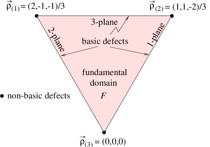
Figure 1: The fundamental domain ${\cal F}$ for $SU(3)$. The extremal points of the simplex ${\cal F}$ correspond to the center elements.

On the boundary face opposite to extremal point $\vec{\rho}_{(\sigma)}$ the inequality $\rho_{\sigma}\leq\rho_{\sigma+1}$ in (LABEL:ordering) becomes an equality. We call this $(N\!-\!2)$-dimensional face the $\sigma$-plane. If $\vec{\rho}$ lies on several $\sigma$-planes, then $D(\vec{\rho})$ and hence ${\cal P}$ has several coinciding eigenvalues, see below. From now on we shall assume that the argument $\vec{\rho}(\vec{x})$ of $D$ lies in the fundamental domain. Then (LABEL:diagonalization) assigns a unique $\vec{\rho}(\vec{x})$ to each ${\cal P}(\vec{x})$. We shall see that the singularities (so-called defects) in the decomposition (LABEL:diagonalization) occur at points $\vec{x}$ for which $\vec{\rho}(\vec{x})$ is on the boundary of ${\cal F}$.

The diagonalizing matrix $W(\vec{x})$ in (LABEL:diagonalization) is determined only up to right-multiplication with an arbitrary matrix commuting with $D(\vec{x})$

$$W(\vec{x})\longrightarrow W(\vec{x})V(\vec{x})\,,\quad V(\vec{x})D(\vec{x})V^{-1}(\vec{x})=D(\vec{x}).$$

At each point the residual gauge transformations $V(\vec{x})$ form a subgroup of $SU(N)$ which contains the maximal Abelian subgroup $U^{N-1}(1)$ of $SU(N)$. At points where it is just this subgroup we can smoothly diagonalize the Polyakov loop operator. However, at points where it is

$$H\times U^{l}(1)\,,\quad H\,\mbox{non-Abelian}\,,\quad\,\mbox{rank}\,(H)+l=N-1\,,$$

the Polyakov loop ${\cal P}(\vec{x})$ has degenerate eigenvalues and there are obstructions to diagonalizing it smoothly [4, 5, 6]. It is convenient to define the defect manifold

$${\cal D}=\{\vec{x}\in\mbox{\af T}^{3}|\hbox{residual gauge group at }\vec{x}\neq U^{N-1}(1)\}$$

on which the residual gauge symmetry is non-Abelian. A defect ${\cal D}_{p}$ is understood to be a connected subset of ${\cal D}$. In the neighbourhood of a defect the diagonalization is in general not smoothly possible and the gauge fixing will be singular.

Now we classify the various defects arising in our gauge fixing. There is a defect whenever ${\cal P}(\vec{x})$ has degenerate eigenvalues, i.e. when $\vec{\rho}(\vec{x})$ is on the boundary of ${\cal F}$. When $\vec{\rho}(\vec{x})$ lies on only one $\sigma$-plane forming the boundary of ${\cal F}$ then exactly two eigenvalues coincide. We call this a basic $\sigma$-defect. Its residual gauge symmetry group $SU(2)\times U^{N-2}(1)$ is minimally non-Abelian. There are $N$ types of basic $\sigma$-defects. If a defect lies on several, say $k$, $\sigma$-planes, the non-Abelian part $H$ of the residual gauge group has rank $k$. $H$ is generated by the $SU(2)$-subgroups associated to the $\sigma$-planes on which the defect lies.

Away from the defects $W(\vec{x})$ in (LABEL:diagonalization) is unique up to a residual Abelian gauge transformation (LABEL:residual):

$$W(\vec{x})\longrightarrow W(\vec{x})V(\vec{x})\quad\hbox{{with}}\quad V(\vec{x})=e^{-i\lambda(\vec{x})}\in U^{N-1}(1)\quad\hbox{{on}}\quad{\cal D}^{c}:=\mbox{\af T}^{3}\setminus{\cal D}\,.$$

If we append to each point in ${\cal D}^{c}$ the set of all diagonalizing matrices $W(\vec{x})$ we obtain a $U^{N-1}(1)$ principal bundle over ${\cal D}^{c}$. If we can find a smooth global section in this bundle then the diagonalization is smoothly possible outside of the defects, see also [17]. To investigate the structure of the bundle we employ the Abelian $U^{N-1}(1)$ gauge potential, $A_{mag}(\vec{x})$, obtained by projecting the pure gauge $A_{W}=iW^{-1}dW$ onto the Cartan subalgebra,

$$A_{mag}(\vec{x}):=(A_{W})_{c}\,,$$

where the subscript $c$ denotes the diagonal part of $A_{W}(\vec{x})$. This Abelian potential is singular at the defects and on Dirac strings joining the defects. Under a residual gauge transformation (LABEL:diagonalize) the gauge potential transforms as

$$A_{mag}\longrightarrow A_{mag}+i(V^{-1}dV)_{c}=A_{mag}+d\lambda\quad\hbox{{on}}\quad{\cal D}^{c}\,.$$

Since $A_{W}$ is pure gauge, the field strength corresponding to $A_{mag}$ is given by

$$\begin{array}[]{rcl}\displaystyle F_{mag}={\mbox{d}}A_{mag}=i(A_{W}\wedge A_{W})_{c}\,,\end{array}$$ (19)

and it is invariant under residual Abelian gauge transformations.

A defect may carry $N-1$ quantized magnetic charges [18]. For each defect these charges form a matrix $Q_{M}$ in the Cartan subalgebra,

$$Q_{M}=\frac{1}{2\pi}\int\limits_{{\cal S}}F_{mag}\,.$$

Here ${\cal S}$ is a surface surrounding the defect. The charge matrix $Q_{M}$ must satisfy the following quantization condition

$$e^{2\pi iQ_{M}}=1\!\mbox{l}\quad\quad\hbox{{for each defect.}}\quad$$

This is just the standard magnetic charge quantization condition of Goddard et.al [19].

If a defect ${\cal D}_{p}$ divides ${\cal D}^{c}$ into disconnected parts, e.g. a closed wall which may extend over the whole torus $\mbox{\af T}^{3}$, some comments are in order. In this case the surface ${\cal S}_{p}$ surrounding the wall ${\cal D}_{p}$ consists of several connected parts. If the wall defect does not extent over $\mbox{\af T}^{3}$ every part of ${\cal S}_{p}$ has no boundary and we get the above quantization condition, see also [20]. If the wall-defect extends over $\mbox{\af T}^{3}$ then each part of ${\cal S}_{p}$ also extends over $\mbox{\af T}^{3}$. But since $F_{mag}$ is periodic on $\mbox{\af T}^{3}$ the integral of $F_{mag}$ over each part of ${\cal S}_{p}$ is again quantized, since we get no contributions to the magnetic charge from the ‘boundary’ of the torus.

Depending on the residual gauge symmetry in the defects we get different types of magnetic monopoles. This is most elegantly expressed if we introduce the simple roots and the lowest root,

$${\alpha_{(j)}}=\hbox{diag}\big{(}\overbrace{0,\dots,0}^{j-1},1,-1,0\dots 0\big{)}\;\quad\hbox{{and}}\quad\;\alpha_{(N)}=\hbox{diag}\big{(}-1,0,\dots,0,1\big{)}.$$

The simple roots are dual to the fundamental weights introduced earlier,

$$\mbox{tr}\,\big{(}{\alpha_{(i)}}\cdot{\mu_{(j)}}\big{)}=\delta_{ij},\quad i,j\in\{1,\dots,N\!-\!1\}.$$

We have seen that to each basic $\sigma$-defect there is an associated residual symmetry group $SU(2)$. The root $\alpha_{(\sigma)}$ generates the diagonal subgroup of this $SU(2)$. Below we shall see that a basic $\sigma$-defect has magnetic charge

$$Q_{M}=m\,\alpha_{(\sigma)}\quad\hbox{{with}}\quad m\in\mbox{\af Z},\qquad\sigma\in\{1,\dots,N\}.$$

If a defect lies on two or more $\sigma$-planes then $Q_{M}$ is an integer combination of the corresponding $\alpha_{(\sigma)}$,

$$Q_{M}=\sum_{\sigma=1}^{N}m_{\sigma}\alpha_{(\sigma)},\qquad m_{\sigma}\in\mbox{\af Z},\qquad m_{\sigma}=0\,\,\quad\hbox{{if defect is not on $\sigma$-plane.}}\quad$$

The $m_{\sigma}$ are not overdetermined because a defect can maximally lie on $N-1$ of the $\sigma$-planes. The charge matrix $Q_{M}$ lies in the Cartan-subalgebra of the non-Abelian part $H$ of the residual symmetry group associated to the defect.

We shall also prove the following relation between the instanton number and the magnetic charges of defects of one type:

$$q=-\sum_{\tiny\hbox{$\sigma$-defects}}m_{\sigma}\,.$$

Since (LABEL:instantonno) is valid for all types of defect it is immediately obvious that for $|q|>0$ every type of defect must be present. For example, in the case $q=-1$ the total magnetic charge of a given type of defect is unity. The simplest (i.e. minimal) way of achieving this would be to have exactly one monopole of each type. One is tempted to speculate whether this minimal monopole content is always achieved for minimal action configurations, i.e. self-dual solutions. Indeed, in the recent construction of the general $q=1$ caloron solutions (i.e. instantons on $S^{1}\times\mbox{\af R}^{3}$) [21] each instanton has exactly $N$ monopole ‘constituents’. Since the magnetic field strength $F_{mag}$ lives on the compact manifold $\mbox{\af T}^{3}$ it follows that we have overall magnetic charge neutrality:

$$\sum_{\tiny\hbox{all defects}}Q_{M}=0\,.$$

This also follows immediately from (LABEL:magneticcharge) and (LABEL:instantonno); in that it is apparent that the total magnetic charge must be proportional to $\sum_{\sigma=1}^{N}\alpha_{(\sigma)}=0$.

To derive the results (LABEL:magneticcharge,LABEL:instantonno) we assume that inside a defect the residual gauge group is uniform. This assumption is made to avoid the complication of ‘defects within defects’. Our arguments are based on the observation that

$$\mbox{tr}\,\,\big{(}P^{-1}dP\big{)}^{3}={\mbox{d}}{\cal A}^{(\sigma)},\qquad\sigma=1,\ldots,N$$

where the $2$-forms are

$${\cal A}^{(\sigma)}=-6\,\mbox{tr}\,\left[A_{W}\wedge A_{W}\left(\log D-2\pi i\mu_{(\sigma)}\right)\right]+3\,\mbox{tr}\,\left[A_{W}D^{-1}\wedge A_{W}D\right]\,.$$

These forms are smooth outside the defects, because they are invariant under the residual Abelian gauge transformations (LABEL:diagonalize). However, ${\cal A}^{(\sigma)}$ can smoothly be continued into all but the $\sigma$-defects [22].

Now we make use of (LABEL:aab) to relate the magnetic charges of the $\sigma$-defects to the instanton number. Away from such defects ${\cal A}^{(\sigma)}$ is regular. Now we surround each $\sigma$-defect with a closed surface ${\cal S}$ and pick a two form ${\cal A}^{(\rho)}$ which is smooth inside ${\cal S}$, see fig.2. Since a defect can not lie on all faces constituting the boundary of ${\cal F}$ there is always at least one such regular two form with $\rho\neq\sigma$.

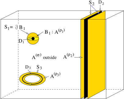
Figure 2: We must choose two forms ${\cal A}^{(\rho_{p})}$ which are regular inside closed $2$-surfaces $S_{p}$ containing $\sigma$-defects $D_{p}$. Shown are $3$ topologically distinct defects: a point-, ring- and wall-defect.

With (LABEL:polloopindex,LABEL:aab) the instanton number reads

$$q=\frac{1}{24\pi^{2}}\int\limits_{\scriptscriptstyle\rm{outside}}d{\cal A}^{(\sigma)}+\frac{1}{24\pi^{2}}\sum_{p}\int\limits_{{\cal B}_{p}}d{\cal A}^{(\rho_{p})}=\frac{1}{24\pi^{2}}\sum_{p}\int\limits_{{\cal S}_{p}}\big{(}{\cal A}^{(\rho_{p})}-{\cal A}^{(\sigma)}\big{)},$$

where, since the $2$-forms are periodic on $\mbox{\af T}^{3}$, we get no contributions from the ‘boundary of the torus’. Using (LABEL:a) we obtain

$${\cal A}^{(\rho)}-{\cal A}^{(\sigma)}={12\pi i}\,\mbox{tr}\,\Big{(}A_{W}\wedge A_{W}\,\big{(}\mu_{(\rho)}-\mu_{(\sigma)}\big{)}\Big{)}\,.$$

Since the magnetic field $F_{mag}$ is the projection to the Cartan of $iA_{W}\wedge A_{W}$ we find

$${\cal A}^{(\rho)}-{\cal A}^{(\sigma)}={12\pi}\mbox{tr}\,\,\Big{(}F_{mag}\,\big{(}\mu_{(\rho)}-\mu_{(\sigma)}\big{)}\Big{)}$$

and end up with

$$q=\sum_{{\cal D}_{p}}\mbox{tr}\,\Big{(}Q_{M}\,\big{(}\mu_{(\rho_{p})}-\mu_{(\sigma)}\big{)}\Big{)},$$

where we used (LABEL:magncharge). The sum extends over all $\sigma$-defects.

Let us have a closer look at the contribution

$$\mbox{tr}\,\Big{(}Q_{M}\,\big{(}\mu_{(\rho)}-\mu_{(\sigma)}\big{)}\Big{)}$$

of a given basic $\sigma$-defect with minimal non-Abelian centralizer. Then all ${\cal A}^{(\rho)}$ with $\rho\neq\sigma$ are regular at the defect and (LABEL:onedefect) must not depend on $\mu_{(\rho)}$. By noting that the fundamental weights are dual to the simple roots we see at once that $Q_{M}$ must be proportional to $\alpha_{(\sigma)}$. With the quantization conditions (LABEL:quantbed) we arrive at

$$Q_{M}=m_{\sigma}\,\alpha_{(\sigma)}\,\qquad m_{\sigma}\in\mbox{\af Z}.$$

With (LABEL:qmag) a basic $\sigma$-defect contributes $-m_{\sigma}$ to the instanton number.

A non-basic defect on the $\sigma$-plane must also lie on one of the other boundary-planes, say the $\rho$-plane. Then we must not take the corresponding singular ${\cal A}^{(\rho)}$ in (LABEL:instantonnu) or $\mu_{(\rho)}$ in (LABEL:onedefect). We see that $Q_{M}$ may be an integer linear combination of $\alpha_{(\sigma)}$ and $\alpha_{(\rho)}$. If the defect lies on several $\sigma$-planes (LABEL:charge-on-0-plane) holds. The representation (LABEL:charge-on-0-plane) for the magnetic charge is unique. Note that the results (LABEL:charge-on-0-plane,LABEL:instantonno) are also correct in the presence of wall defects.

In [15, 4] it has been shown that the (singular) gauge fixing

$$A_{0}=\big{(}A_{0}(\vec{x})\big{)}_{c}$$

can be supplemented by additional gauge fixing conditions on the diagonal parts of $A_{1},A_{2}$ and $A_{3}$. This gauge can be achieved and is unique. One can show [23] that field dependent part of the Fadeev-Popov determinant associated to these conditions is

$$\det\,D_{0}|_{{\cal H}^{\perp}},\qquad D_{0}=\partial_{0}-i[A_{0},\,.\,].$$

Here ${\cal H}^{\perp}$ is the space orthogonal to the Cartan subalgebra. With (LABEL:gfanull,LABEL:D) our gauge fixed $A_{0}$ is diagonal and time-independent,

$$A_{0}=-{i\over\beta}\log D(\vec{x})={2\pi\over\beta}\,\hbox{diag}\,\big{(}\rho_{1}(\vec{x}),\dots,\rho_{N}(\vec{x})\big{)},$$

and $\vec{\rho}(\vec{x})$ lies in the fundamental domain ${\cal F}$. With

$$D_{0}\psi=D^{\xi^{0}}\partial_{0}\big{(}D^{-\xi^{0}}\psi D^{\xi^{0}}\big{)}D^{-\xi^{0}},\qquad\xi^{0}=x^{0}/\beta.$$

the eigenvalue problem $D_{0}\psi=\lambda\psi$ on the space of time-periodic functions results in the following simple equation for $\chi=D^{-\xi^{0}}\psi D^{\xi^{0}}$:

$$\partial_{0}\chi=\lambda\chi,\quad\hbox{{with boundary conditions}}\quad\chi(x^{0}+\beta)=D^{-1}(\vec{x})\chi(x^{0})D(\vec{x}).$$

Now it is not difficult to prove [14, 24] that

$$\det\,D_{0}|_{{\cal H}^{\perp}}=C\;\prod_{1\leq i<j\leq N}\sin^{2}\big{\{}\pi(\rho_{i}(\vec{x})-\rho_{j}(\vec{x}))\big{\}}$$

with a field-independent constant $C$. It is just the reduced Haar measure of $SU(N)$ [25]. On the basic defects where either two $\rho$’s are equal or $\rho_{1}\!-\!\rho_{N}=1$ the Fadeev-Popov determinant has a root of multiplicity $2$. More generally, on a (non-basic) defect where the residual symmetry group is $H\times U^{l}(1)$ the determinant has a root of multiplicity $\,\mbox{dim}\,(H)-\,\mbox{rank}\,(H)$. In particular, at the center elements the determinant has a root of multiplicity $N(N-1)$. In other words, the multiplicity of the Fadeev-Popov determinant at a defect is equal to the number of non-diagonal generators of the residual gauge group at this defect. For a given $\vec{x}$ the corresponding zero modes $\chi$ of $D_{0}|_{{\cal H}^{\perp}}$ are just the elements in $H\cap{\cal H}^{\perp}$.

Since the Fadeev-Popov determinant vanishes on the boundary of ${\cal F}$ we conclude, that the defects lie on the Gribov horizon. However, although the boundary of ${\cal F}$ has common points with the Gribov horizon they are not the same. Because of the gauge fixing conditions on the spatial components of the gauge potential the fundamental domain is smaller (has lower dimension) than the domain bounded by the horizon.

References

- [1] K.G. Wilson, Phys. Rev. D10 (1974) 2445.
- [2] A.M. Polyakov, Phys. Lett. 72B (1978) 477; L. Susskind, Phys. Rev. D20 (1979) 2610.
- [3] G. ’t Hooft, Nucl. Phys. B153 (1979) 141; Acta Phys. Austria CA Suppl. XXII (1980) 1063; Phys. Scr. 24 (1981) 841.
- [4] C. Ford, U.G. Mitreuter, T. Tok, A. Wipf and J.M. Pawlowski, Annals Phys. 269 (1998) 26.
- [5] G. ’t Hooft, Nucl. Phys. B190 (1981) 455.
- [6] A.S. Kronfeld, G. Schierholz and U.J. Wiese, Nucl. Phys. B293 (1987) 461.
- [7] H. Reinhardt, Nucl. Phys. B503 (1997) 505.
- [8] O. Jahn and F. Lenz, Phys. Rev. D58 (1998) 085006.
- [9] N. Christ and R. Jackiw, Phys. Lett. 91B (1980) 228.
- [10] D.J. Gross, R.D. Pisarski and L.G. Yaffe, Rev. Mod. Phys. 53 (1981) 43.
- [11] U.G. Mitreuter, J.M. Pawlowski and A. Wipf, Nucl. Phys. B514 (1998) 381.
- [12] A. Gonzalez-Arroyo, Yang-Mills Fields on the 4-dimensional torus. Part I: Classical Theory, preprint FTUAM-97/18, hep-th/9807108.
- [13] P. van Baal, Comm. Math. Phys. 85 (1982) 529.
- [14] N. Weiss, Phys. Rev. D24 (1981) 475.
- [15] E. Langmann, M. Salmhofer and A. Kovner, Mod. Phys. Lett. A9 (1994) 2913.
- [16] F. Lenz, H.W.L. Naus and M. Thies, Annals Phys. 233 (1994) 317.
- [17] H. W. Grießhammer, Magnetic Defects Signal Failure of Abelian Projection Gauges in QCD, preprint FAU-TP3-97/6, hep-ph/9709462.
- [18] G. ’t Hooft, Nucl. Phys. B79 (1974) 276; A.M. Polyakov, JETP lett. 20 (1974) 194.
- [19] P. Goddard, J. Nuyts and D. Olive, Nucl. Phys. B125 (1977) 1.
- [20] M. Quandt, H. Reinhardt and A. Schafke, Magnetic Monopoles and Topology of Yang-Mills Theory in Polyakov Gauge, UNITU-THEP-17-1998, hep-th/9810088.
- [21] T.C. Kraan and P. van Baal, Phys. Lett. B435 (1998) 389.
- [22] C. Ford, T. Tok and A. Wipf, Abelian Projection on the torus for general gauge groups, FSUJ-TPI-98-11, hep-th/9809209.
- [23] F. Bruckmann, T. Heinzl, T. Tok and A. Wipf, to appear.
- [24] H. Reinhardt, Mod. Phys. Lett. A11 (1996) 2451.
- [25] H. Weyl, The classical groups, Princeton University Press, Princeton, NJ, 1973.