UT-Komaba 98-12 DPNU-98-22 OU-HET 298 November 1998

Dynamical Aspects of Large $N$ Reduced Models

Tomohiro Hotta¹⁾, Jun Nishimura²⁾ and Asato Tsuchiya^3)
1) Institute of Physics, University of Tokyo,
Komaba, Meguro-ku, Tokyo 153-8902, Japan

²⁾ Department of Physics, Nagoya University,
Chikusa-ku, Nagoya 464-8602, Japan

³⁾ Department of Physics, Graduate School of Science,
Osaka University, Toyonaka, Osaka 560-0043, Japan

We study the large $N$ reduced model of $D$-dimensional Yang-Mills theory with special attention to dynamical aspects related to the eigenvalues of the $N\times N$ matrices, which correspond to the space-time coordinates in the IIB matrix model. We first put an upper bound on the extent of space time by perturbative arguments. We perform a Monte Carlo simulation and show that the upper bound is actually saturated. The relation of our result to the SSB of the U(1)^D symmetry in the Eguchi-Kawai model is clarified. We define a quantity which represents the uncertainty of the space-time coordinates and show that it is of the same order as the extent of space time, which means that a classical space-time picture is maximally broken. We develop a $1/D$ expansion, which enables us to calculate correlation functions of the model analytically. The absence of an SSB of the Lorentz invariance is shown by the Monte Carlo simulation as well as by the $1/D$ expansion.

1 Introduction

Large $N$ reduced models, which are the zero-volume limit of gauge theories, have been developed for studying the large $N$ limit of gauge theories [1, 2, 3, 4, 5]. Recently the (partially) reduced models have been revived in the context of nonperturbative formulations of string theory [6, 7]. The IIB matrix model [7, 8, 9], which is the reduced model of ten-dimensional supersymmetric Yang-Mills theory, is expected to be a nonperturbative formulation of superstring theory. It is hoped that all the fundamental issues including the origin of the space-time dimensionality can be understood by studying the dynamics of this model.

Aiming at such an end, we study the large $N$ reduced model of Yang-Mills theory, which we call as the “bosonic model”, since it is nothing but the bosonic part of the IIB matrix model. The action of the bosonic model is given by

$$S=-\frac{1}{4g^{2}}\mbox{tr}([A_{\mu},A_{\nu}]^{2}),$$ (1.1)

where $A_{\mu}$ $(\mu=1,\cdots,D)$ are $N\times N$ traceless hermitian matrices. The partition function is given by

$$Z=\int\mbox{d}A~{}\mbox{e}^{-S},$$ (1.2)

where the measure $\mbox{d}A$ is defined by

$$\mbox{d}A=\prod_{\mu=1}^{D}\left[\prod_{i=1}^{N}\mbox{d}(A_{\mu})_{ii}\delta\left(\sum_{i=1}^{N}(A_{\mu})_{ii}\right)\prod_{i<j}\mbox{d}\mbox{Re}(A_{\mu})_{ij}\mbox{d}\mbox{Im}(A_{\mu})_{ij}\right].$$ (1.3)

In Ref. [10], the value of the partition function of this model has been numerically evaluated and found to be finite for $N\geq 4$ when $D=3$, for $N\geq 3$ when $D=4$, and for $N\geq 2$ when $D\geq 5$, which means that in the large $N$ limit, the model is well-defined for $D\geq 3$ without any regularizations. This property, together with the fact that the action is homogeneous with respect to $A_{\mu}$, enables us to absorb the coupling constant $g$ by rescaling $A_{\mu}^{\prime}=\frac{1}{\sqrt{g}}A_{\mu}$. Hence $g$ is nothing but a scale parameter like the lattice spacing in lattice gauge theories, and the dependence of expectation values on $g$ is determined on dimensional grounds, which is also the case for the IIB matrix model [9]. This is in striking contrast to the ordinary Yang-Mills theory before being reduced, where the parameter $g$ is the coupling constant, which is independent of the scale parameter.

We investigate dynamical aspects of the model related to the eigenvalues of $A_{\mu}$, which correspond to the space-time coordinates in the IIB matrix model. One of the most important quantities is the extent of space time defined by $R=\sqrt{\langle\frac{1}{N}\mbox{tr}(A^{2})\rangle}$. Since $R$ should be proportional to $\sqrt{g}$ on dimensional grounds, we parameterize its large $N$ behavior as $R\sim\sqrt{g}N^{\omega}$. In the IIB matrix model, the value of $\omega$ plays an important role when we deduce the space-time dimension, which is to be determined dynamically within the model. We determine the value of $\omega$ for the bosonic model. We first obtain an upper bound on $\omega$, namely $\omega\leq\frac{1}{4}$ by perturbative arguments. The first argument is based on a perturbative calculation of the effective action for the eigenvalues of $A_{\mu}$. The second one is based on exact relations among correlation functions derived as Schwinger-Dyson equations. We evaluate the correlation functions as a perturbative expansion and estimate the large $N$ behavior of each term, from which we extract an upper bound on the extent of space time by requiring that the Schwinger-Dyson equations should be satisfied if we take all the terms of the perturbative expansion into account. We then perform a Monte Carlo simulation and find that $\omega=\frac{1}{4}$, which means that the upper bound given through perturbative arguments is actually saturated. This means that the perturbative estimation of the large $N$ behavior of correlation functions is valid, which is also confirmed directly by the Monte Carlo simulation. We further clarify the relation of our result concerning the extent of space time to the SSB of the U(1)^D symmetry in the Eguchi-Kawai model.

The space time which is generated dynamically in the IIB matrix model is not classical, since $A_{\mu}$’s which are given dynamically are non-commutative generically. To what extent a classical space-time picture is broken is therefore an important issue to address. For this purpose, we define a quantity which represents the uncertainty of the space-time coordinates. We determine its large $N$ behavior for the bosonic model and show that it is of the same order as the extent of space time, which means that the classical space-time picture is maximally broken in the bosonic model.

In the IIB matrix model, the (ten-dimensional) Lorentz invariance should be broken spontaneously if the space time generated dynamically is to be four-dimensional. We define an order parameter for the SSB of the Lorentz invariance. We show, for the bosonic model, that the order parameter vanishes in the large $N$ limit, and hence the Lorentz invariance is not spontaneously broken.

As a method complementary to the Monte Carlo simulation, we develop a $1/D$ expansion, which enables us to calculate correlation functions of the model analytically. To all orders of the $1/D$ expansion, we determine the large $N$ behavior of correlation functions, which agrees with the one obtained by the perturbation theory and the Monte Carlo simulation. We also prove that the large $N$ factorization property holds for the correlation functions. In order to confirm the validity of the $1/D$ expansion for studying the large $N$ limit of the model for finite $D$, we perform explicit calculations of correlation functions up to the next-leading terms in $1/D$ and compare the results with the Monte Carlo data. We conclude that there is no phase transition at some finite $D$ and that the $1/D$ expansion is valid for any $D\geq 3$.

This paper is organized as follows. In Section 2, we focus on the extent of space time. We first put an upper bound on $\omega$, namely $\omega\leq\frac{1}{4}$ by perturbative arguments. We then show that the upper bound is actually saturated by a Monte Carlo simulation. We further clarify the relation of our result to the SSB of the U(1)^D symmetry in the Eguchi-Kawai model. In Section 3, we show that a classical space-time picture is maximally broken in the bosonic model. In Section 4, we develop a $1/D$ expansion, with which we determine the large $N$ behavior of correlation functions. In Section 5, the absence of an SSB of the Lorentz invariance is shown by the Monte Carlo simulation as well as by the $1/D$ expansion. Section 6 is devoted to summary and discussion.

2 The extent of space time

2.1 Perturbative arguments

2.1.1 Upper bound from the effective action

We first start by decomposing $A_{\mu}$ into its eigenvalues $\lambda_{i\mu}$ and the angular part $V_{\mu}$ as [4]

$$A_{\mu}=V_{\mu}\Lambda_{\mu}V_{\mu}^{\dagger},$$ (2.1)

where $\Lambda_{\mu}=\mbox{diag}(\lambda_{\mu 1},\cdots,\lambda_{\mu N})$ and $V_{\mu}$ is a unitary matrix. Since $A_{\mu}$ is traceless, we have $\sum_{i}\lambda_{\mu i}=0$. The effective action $W(\lambda)$ for the eigenvalues can be defined by

$$\mbox{e}^{-W(\lambda)}=\int\mbox{d}A\int\mbox{d}V\left[\prod_{\mu}\left\{\prod_{i>j}(\lambda_{\mu i}-\lambda_{\mu j})^{2}\right\}\delta(A_{\mu}-V_{\mu}\Lambda_{\mu}V_{\mu}^{\dagger})\right]~{}\mbox{e}^{-S}.$$ (2.2)

The VEV of an operator ${\cal O}$ can be written as

$$\langle{\cal O}\rangle=\frac{\int\mbox{d}\lambda\;{\cal O}(\lambda)\;\mbox{e}^{-W(\lambda)}}{\int\mbox{d}\lambda\;\mbox{e}^{-W(\lambda)}},$$ (2.3)

where ${\cal O}(\lambda)$ is defined by

$${\cal O}(\lambda)=\frac{\int\mbox{d}A\int\mbox{d}V\left[\prod_{\mu}\left\{\prod_{i>j}(\lambda_{\mu i}-\lambda_{\mu j})^{2}\right\}\delta(A_{\mu}-V_{\mu}\Lambda_{\mu}V_{\mu}^{\dagger})\right]~{}{\cal O}~{}\mbox{e}^{-S}}{\int\mbox{d}A\int\mbox{d}V\left[\prod_{\mu}\left\{\prod_{i>j}(\lambda_{\mu i}-\lambda_{\mu j})^{2}\right\}\delta(A_{\mu}-V_{\mu}\Lambda_{\mu}V_{\mu}^{\dagger})\right]~{}\mbox{e}^{-S}}.$$ (2.4)

We can perform a perturbative expansion with respect to $g^{2}$ regarding $\lambda_{\mu i}$ as external fields. The perturbation theory is valid when $\lambda_{i}$’s are widely separated, as we will see shortly.

We first integrate out $V_{\mu}$ perturbatively around the unit matrix either in (2.2) or in (2.4). We find that the van der Monde determinants are cancelled out and obtain the following constraints [4].

$$d_{\mu i}=\lambda_{\mu i}-\sum_{j\neq i}\frac{a_{\mu ij}a_{\mu ji}}{\lambda_{\mu i}-\lambda_{\mu j}}+O(a^{3}),$$ (2.5)

where $d_{\mu i}$ and $a_{\mu ij}$ are the diagonal parts and the off-diagonal parts of $A_{\mu}$ respectively.

Since the quadratic term in $a$ of the action is

$$S_{2}=-\frac{1}{2g^{2}}\{\mbox{tr}([\lambda_{\mu},a_{\nu}]^{2})-\mbox{tr}([\lambda_{\mu},a_{\mu}]^{2})\},$$ (2.6)

we have to fix the gauge. Here we put the following gauge fixing term and the corresponding Faddeev-Popov ghost term.

$$S_{g.f.} = -\frac{1}{2g^{2}}\mbox{tr}([\lambda_{\mu},a_{\mu}]^{2})$$ (2.7)

$$S_{gh} = -\frac{1}{g^{2}}\mbox{tr}([\lambda_{\mu},b][d_{\mu}+a_{\mu},c])$$ (2.8)

The total action $S^{\prime}=S+S_{g.f.}+S_{gh}$ can be written as follows.

$$S^{\prime} = S_{2}^{\prime}+S_{int},$$ (2.9)

$$S_{2}^{\prime} = \frac{1}{g^{2}}\sum_{i\neq j}\left(\frac{1}{2}(\lambda_{i}-\lambda_{j})^{2}a_{\mu ji}a_{\mu ij}+b_{ji}(\lambda_{i}-\lambda_{j})^{2}c_{ij}\right),$$ (2.10)

$$S_{int} = -\frac{1}{g^{2}}\left[\mbox{tr}\left([\lambda_{\mu},a_{\nu}][a_{\mu},a_{\nu}]+\frac{1}{4}[a_{\mu},a_{\nu}]^{2}-b[\lambda_{\mu},[a_{\mu},c]]\right)\right.$$ (2.11)

$$+\sum_{i\neq j,i\neq k}\left\{\sum_{\mu,\nu}\left(2\frac{\lambda_{\mu i}-\lambda_{\mu j}}{\lambda_{\mu i}-\lambda_{\mu k}}a_{\mu ik}a_{\mu ki}a_{\nu ij}a_{\nu ji}\right.\right.$$

$$\left.-\frac{\lambda_{\nu i}-\lambda_{\nu j}}{\lambda_{\mu i}-\lambda_{\mu k}}a_{\mu ik}a_{\mu ki}(a_{\mu ij}a_{\nu ji}+a_{\mu ji}a_{\nu ij})\right)$$

$$\left.\left.+\sum_{\mu}\frac{\lambda_{\mu i}-\lambda_{\mu j}}{\lambda_{\mu i}-\lambda_{\mu k}}a_{\mu ik}a_{\mu ki}(b_{ij}c_{ji}+b_{ji}c_{ij})\right\}+O(a^{5})\right]$$

From (2.10), we can read off the propagators as

$$\langle\!\langle a_{\mu ij}a_{\nu kl}\rangle\!\rangle = g^{2}\delta_{\mu\nu}\delta_{il}\delta_{jk}\frac{1}{(\lambda_{i}-\lambda_{j})^{2}},$$

$$\langle\!\langle c_{ij}b_{kl}\rangle\!\rangle = g^{2}\delta_{il}\delta_{jk}\frac{1}{(\lambda_{i}-\lambda_{j})^{2}},$$ (2.12)

where the symbol $\langle\!\langle\cdots\rangle\!\rangle$ is defined by

$$\langle\!\langle{\cal O}\rangle\!\rangle=\frac{\int\mbox{d}a\mbox{d}b\mbox{d}c~{}{\cal O}~{}\mbox{e}^{-S_{2}^{\prime}}}{\int\mbox{d}a\mbox{d}b\mbox{d}c~{}\mbox{e}^{-S_{2}^{\prime}}}.$$ (2.13)

The interaction vertices can be read off from $S_{int}$.

The one-loop effective action $W_{1}(\lambda)$ for $\lambda_{\mu i}$ is given by

$$W_{1}(\lambda)=(D-2)\sum_{i<j}\log(\lambda_{i}-\lambda_{j})^{2},$$ (2.14)

which is an $O(N^{2})$ quantity and gives a logarithmic attractive potential between all the pairs of $\lambda_{i}$. If the $\lambda_{i}$’s are sufficiently separated from one another, the one-loop effective action (2.14) dominates and higher loop corrections can be neglected.

We can therefore examine the convergence of the integration over $A_{\mu}$ in (1.2) in the infrared region, where the eigenvalues are far apart, by using the one-loop effective action (2.14). The power of $\lambda$ coming from the one-loop effective action is $-(D-2)N(N-1)$, while the one coming from the measure is $D(N-1)$. If and only if the sum of the powers is strictly negative, the integration over $\lambda_{\mu i}$ converges in the infrared region. Thus, we obtain the condition for the infrared convergence as

$$N>\frac{D}{D-2}.$$ (2.15)

Let us next discuss the behavior of the model in the ultraviolet region, where some pairs of the eigenvalues are close to each other. Looking at the one-loop effective action (2.14), one might argue that there might be an ultraviolet divergence. The two-loop effective action (2.23), which we calculate later, actually shows even a severer divergence for coinciding eigenvalues, and the higher loop one considers, the severer divergence one encounters. However, this is simply due to the fact that the perturbative expansion is no more valid in the ultraviolet region, and does not imply a real divergence of the model. Rather, one should look at the partition function before performing the perturbative expansion:

$$Z=\int\mbox{d}\Lambda\int\mbox{d}V\left[\prod_{\mu}\left\{\prod_{i>j}(\lambda_{\mu i}-\lambda_{\mu j})^{2}\right\}\right]~{}\mbox{e}^{-S[V_{\mu}\Lambda_{\mu}V_{\mu}^{\dagger}]},$$ (2.16)

where one sees no source of divergence for coinciding eigenvalues.

Therefore the model is well defined if and only if the condition (2.15) is satisfied. This is in agreement with the results obtained by a numerical evaluation of the value of the partition function [10]. As far as the large $N$ limit is concerned, the bosonic model is well defined for any $D\geq 3$.

Figure 1: The diagrams we have to consider to obtain the two-loop corrections to the effective action for $\lambda_{\mu i}$. The wavy line corresponds to $a_{\mu ij}$ and the dashed line corresponds to the $b$,$c$-ghosts.

As we have seen above, if $\lambda_{i}$’s are widely separated, the $\lambda_{i}$’s attract one another due to the logarithmic attractive potential induced by the one-loop calculation, and the space time shrinks until the dominance of the one-loop effective action no more holds. This means that we can put an upper bound on the extent of the distribution of $\lambda_{i}$ by considering higher loop corrections to the effective action.

Let us calculate the two-loop corrections. The diagrams we have to evaluate are shown in Fig. 1. The diagram (a) is evaluated as follows.

$$(\mbox{a}) = \frac{1}{g^{2}}\left\langle\!\!\left\langle\frac{1}{2}\sum_{ijkl}(a_{\mu ij}a_{\nu jk}a_{\mu kl}a_{\nu li}-a_{\mu ij}a_{\mu jk}a_{\nu kl}a_{\nu li})\right.\right.$$ (2.17)

$$+\sum_{i\neq j,i\neq k}\sum_{\mu,\nu}\left(2\frac{\lambda_{\mu i}-\lambda_{\mu j}}{\lambda_{\mu i}-\lambda_{\mu k}}a_{\mu ik}a_{\mu ki}a_{\nu ij}a_{\nu ji}\right.$$

$$\left.\left.\left.-\frac{\lambda_{\nu i}-\lambda_{\nu j}}{\lambda_{\mu i}-\lambda_{\mu k}}a_{\mu ik}a_{\mu ki}a_{\mu ij}a_{\nu ji}-\frac{\lambda_{\nu i}-\lambda_{\nu j}}{\lambda_{\mu i}-\lambda_{\mu k}}a_{\mu ik}a_{\mu ki}a_{\mu ji}a_{\nu ij}\right)\right\rangle\!\!\right\rangle$$

$$= \frac{1}{g^{2}}\left[\sum_{ijkl}\frac{1}{2}(\langle\!\langle a_{\mu ij}a_{\nu jk}\rangle\!\rangle\langle\!\langle a_{\mu kl}a_{\nu li}\rangle\!\rangle-\langle\!\langle a_{\mu ij}a_{\mu jk}\rangle\!\rangle\langle\!\langle a_{\nu kl}a_{\nu li}\rangle\!\rangle)\right.$$

$$+\sum_{ijk}\sum_{\mu,\nu}\left\{2\frac{\lambda_{\mu i}-\lambda_{\mu j}}{\lambda_{\mu i}-\lambda_{\mu k}}(\langle\!\langle a_{\mu ik}a_{\mu ki}\rangle\!\rangle\langle\!\langle a_{\nu ij}a_{\nu ji}\rangle\!\rangle+\langle\!\langle a_{\mu ik}a_{\nu ji}\rangle\!\rangle\langle\!\langle a_{\mu ki}a_{\nu ij}\rangle\!\rangle)\right.$$

$$-\frac{\lambda_{\nu i}-\lambda_{\nu j}}{\lambda_{\mu i}-\lambda_{\mu k}}(\langle\!\langle a_{\mu ik}a_{\mu ki}\rangle\!\rangle\langle\!\langle a_{\mu ij}a_{\nu ji}\rangle\!\rangle+\langle\!\langle a_{\mu ik}a_{\nu ji}\rangle\!\rangle\langle\!\langle a_{\mu ki}a_{\mu ij}\rangle\!\rangle)$$

$$\left.\left.-\frac{\lambda_{\nu i}-\lambda_{\nu j}}{\lambda_{\mu i}-\lambda_{\mu k}}(\langle\!\langle a_{\mu ik}a_{\mu ki}\rangle\!\rangle\langle\!\langle a_{\mu ji}a_{\nu ij}\rangle\!\rangle+\langle\!\langle a_{\mu ik}a_{\mu ji}\rangle\!\rangle\langle\!\langle a_{\mu ki}a_{\nu ij}\rangle\!\rangle)\right\}\right]$$

$$= -\frac{g^{2}}{2}D(D-1)\sum_{i\neq j,i\neq k}\frac{1}{(\lambda_{i}-\lambda_{j})^{2}(\lambda_{i}-\lambda_{k})^{2}}$$

$$+2g^{2}(D-1)\sum_{i\neq j,i\neq k}\sum_{\mu}\frac{\lambda_{\mu i}-\lambda_{\mu j}}{\lambda_{\mu i}-\lambda_{\mu k}}\frac{1}{(\lambda_{i}-\lambda_{j})^{2}(\lambda_{i}-\lambda_{k})^{2}}.$$

Defining

$$I_{1} = \sum_{i\neq j,j\neq k,k\neq i}\frac{1}{(\lambda_{i}-\lambda_{j})^{2}(\lambda_{i}-\lambda_{k})^{2}},$$ (2.18)

$$I_{2} = \sum_{i\neq j}\frac{1}{(\lambda_{i}-\lambda_{j})^{4}},$$ (2.19)

$$I_{3} = \sum_{\mu}\sum_{i\neq j,i\neq k,j\neq k}\frac{\lambda_{\mu i}-\lambda_{\mu j}}{\lambda_{\mu i}-\lambda_{\mu k}}\frac{1}{(\lambda_{i}-\lambda_{j})^{2}(\lambda_{i}-\lambda_{k})^{2}},$$ (2.20)

we can write the above result as

$$(\mbox{a})=g^{2}\left\{-\frac{1}{2}D(D-1)I_{1}+\frac{3}{2}D(D-1)I_{2}+2(D-1)I_{3}\right\}.$$ (2.21)

The diagrams (b), (c) and (d) can be calculated in the same way. The results are

$$(\mbox{b}) = \frac{3}{2}g^{2}(D-1)I_{1},$$

$$(\mbox{c}) = -\frac{1}{2}g^{2}I_{1},$$

$$(\mbox{d}) = -2g^{2}(DI_{2}+I_{3}).$$ (2.22)

Summing up all these results, we obtain the two-loop effective action as

$$W_{2}(\lambda)=-((\mbox{a})+(\mbox{b})+(\mbox{c})+(\mbox{d}))=g^{2}\left\{\frac{1}{2}(D-2)^{2}I_{1}-\frac{1}{2}D(3D-7)I_{2}-2(D-2)I_{3}\right\}.$$ (2.23)

In order to estimate the order of magnitude of the two-loop effective action, we note that

$$R^{2}=\left\langle\frac{1}{N}\sum_{i}\lambda_{i}^{2}\right\rangle.$$ (2.24)

Assuming that $\lambda_{i}$’s distribute uniformly in a $D$-dimensional ball with the radius $R$ as in Ref. [9], we can estimate the order of magnitude of $I_{1}$ and $I_{2}$ as follows.

$$I_{1} \sim N^{3}\frac{1}{{R}^{3D}}\int\mbox{d}^{D}x~{}\mbox{d}^{D}y~{}\mbox{d}^{D}z~{}\frac{1}{(x-y)^{2}(x-z)^{2}}\sim O\left(\frac{N^{3}}{{R}^{4}}\right).$$ (2.25)

$$I_{2} \sim N^{2}\frac{1}{{R}^{2D}}\int\mbox{d}^{D}x~{}\mbox{d}^{D}y~{}\frac{1}{(x-y)^{4}}\sim O\left(\frac{N^{2}}{{R}^{4}}\right).$$ (2.26)

Similarly, we can estimate the order of magnitude of $I_{3}$ as $O\left(\frac{N^{3}}{{R}^{4}}\right)$. Therefore the order of magnitude of the two-loop corrections is $O\left(\frac{g^{2}N^{3}}{{R}^{4}}\right)$. By simple power counting, we can see that the $n$-loop corrections are of the order of $O\left(N^{2}\left(\frac{g^{2}N}{{R}^{4}}\right)^{(n-1)}\right)$, in general.

Since the one-loop result for the effective potential can be considered as an $O(N^{2})$ quantity, the higher loop corrections can be neglected as long as $R>\sqrt{g}N^{1/4}$. Thus, we can put an upper bound on $R$ as $R\lesssim\sqrt{g}N^{1/4}$.

2.1.2 Perturbative estimation of correlation functions

In this section, we explain how to estimate the order in $N$ of correlation functions of $A$ through perturbative calculations. We will see that the perturbative estimation is valid if the upper bound on $R$ given in Section 2.1.1 is actually saturated.

Here we perform the integration over $a_{\mu}$ in (2.4) perturbatively as

$${\cal O}(\lambda)=\frac{\int\mbox{d}a\mbox{d}b\mbox{d}c~{}{\cal O}~{}\mbox{e}^{-S^{\prime}}}{\int\mbox{d}a\mbox{d}b\mbox{d}c~{}\mbox{e}^{-S^{\prime}}}.$$ (2.27)

An example of the operator ${\cal O}$ we consider is $\mbox{tr}(A^{2})$. We calculate ${\cal O}(\lambda)$ as a perturbative expansion with respect to $g^{2}$, which gives a loop-wise expansion. We then perform the integration over $\lambda$ for the result of each order of the perturbative expansion of ${\cal O}(\lambda)$ with the Boltzmann factor $\mbox{e}^{-W(\lambda)}$ defined nonperturbatively by (2.2)

As an example, let us consider the perturbative estimation of $\langle\frac{1}{N}\mbox{tr}((A^{2})^{2})\rangle$.

$$\left\langle\frac{1}{N}\mbox{tr}((A^{2})^{2})\right\rangle = \left\langle\frac{1}{N}\sum_{i}(\lambda_{i}^{2})^{2}\right\rangle+\left\langle\frac{1}{N}\sum_{ij}\lambda_{i}^{2}|a_{\mu ij}|^{2}\right\rangle+\cdots$$ (2.28)

$$= \left\langle\frac{1}{N}\sum_{i}(\lambda_{i}^{2})^{2}\right\rangle+\left\langle\frac{1}{N}\sum_{i\neq j}\frac{g^{2}\lambda_{i}^{2}}{(\lambda_{i}-\lambda_{j})^{2}}\right\rangle+\cdots.$$

The order of magnitude of the first and second terms are estimated as $O({R}^{4})$ and $O\left(g^{2}N\right)$, respectively. We can easily see that the $n$-loop corrections are of the order of $O\left({R}^{4}\left(\frac{g^{2}N}{{R}^{4}}\right)^{n}\right)$, in general. Therefore, if the upper bound on $R$ obtained in Section 2.1.1 is actually saturated, i.e., $R\sim\sqrt{g}N^{1/4}$, all the orders of the perturbative expansion give the same order in $N$ and we obtain $\langle\frac{1}{N}\mbox{tr}((A^{2})^{2})\rangle\sim g^{2}N$.

We can generalize the above argument to the correlation functions written as

$$\left\langle\frac{1}{N}\mbox{tr}(\underbrace{A\cdots A}_{p_{1}})\frac{1}{N}\mbox{tr}(\underbrace{A\cdots A}_{p_{2}})\cdots\frac{1}{N}\mbox{tr}(\underbrace{A\cdots A}_{p_{Q}})\right\rangle.$$ (2.29)

If the upper bound on $R$ is actually saturated, the above quantity can be estimated as $(\sqrt{g}N^{1/4})^{P}$, where $P=\sum_{i=1}^{Q}p_{i}$.

In Section 2.2, we calculate $R$ through a Monte Carlo simulation and see that the upper bound on $R$ is saturated and that the perturbative estimation of the large $N$ behavior of correlation functions given above is indeed valid.

2.1.3 Upper bound from Schwinger-Dyson equations

In this section, we provide another way to extract information on the extent of space time $R$. The strategy is to derive exact relations among correlation functions of $A$ through Schwinger-Dyson equations and to evaluate each of the correlation functions by the perturbative method described in Section 2.1.2. By estimating the large $N$ behavior of the correlation functions, we will see that the exact relations can be satisfied only if $R\lesssim\sqrt{g}N^{1/4}$ holds.

We expand $A_{\mu}$ as

$$A_{\mu}=\sum_{a=1}^{N^{2}-1}A_{\mu}^{~{}a}~{}t^{a},\\$$ (2.30)

where $t^{a}$ are the generators of SU$(N)$. We consider the following Schwinger-Dyson equations.

$$0 = \int\mbox{d}A\frac{\partial}{\partial A_{\mu}^{~{}a}}\left(\mbox{tr}(t^{a}A_{\mu})\mbox{e}^{-S}\right),$$ (2.31)

$$0 = \int\mbox{d}A\frac{\partial}{\partial A_{\mu}^{~{}a}}\left(\mbox{tr}(t^{a}A_{\nu}A_{\lambda}A_{\rho})\mbox{e}^{-S}\right).$$ (2.32)

These equations lead to the following exact relations, respectively:

$$(\mbox{i}) ~{}~{}~{}~{}~{}-\langle\mbox{tr}([A_{\mu},A_{\nu}]^{2})\rangle=D(N^{2}-1)g^{2},$$

$$(\mbox{ii}) ~{}~{}~{}~{}~{}-g^{2}\frac{1}{D}\left\{\left(N-\frac{1}{N}\right)(\delta_{\mu\nu}\delta_{\lambda\rho}+\delta_{\mu\rho}\delta_{\nu\lambda})-\frac{1}{N}\delta_{\mu\lambda}\delta_{\nu\rho}\right\}\langle\mbox{tr}(A^{2})\rangle$$

$$~{}~{}~{}~{}~{}~{}~{}~{}~{}~{}=\langle\mbox{tr}(A_{\nu}A_{\lambda}A_{\rho}[A_{\tau},[A_{\mu},A_{\tau}]])\rangle.$$ (2.34)

We estimate the large $N$ behavior of each of the correlation functions which appear in the above equations.

Let us first consider eq. (i). We calculate the leading term of the l.h.s. as follows.

$$-\langle\mbox{tr}[A_{\mu},A_{\nu}]^{2}\rangle \stackrel{{\scriptstyle\rm leading}}{{\simeq}} -2\left\{\langle\mbox{tr}[\lambda_{\mu},a_{\nu}][\lambda_{\mu},a_{\nu}]\rangle-\langle\mbox{tr}[\lambda_{\mu},a_{\nu}][\lambda_{\nu},a_{\mu}]\rangle\right\}$$ (2.35)

$$= 2\left\{\left\langle\sum_{i\neq j}(\lambda_{\mu i}-\lambda_{\mu j})(\lambda_{\mu i}-\lambda_{\mu j})\langle\!\langle a_{\nu ji}a_{\nu ij}\rangle\!\rangle\right\rangle\right.$$

$$~{}~{}~{}~{}~{}-\left.\left\langle\sum_{i\neq j}(\lambda_{\mu i}-\lambda_{\mu j})(\lambda_{\nu i}-\lambda_{\nu j})\langle\!\langle a_{\nu ji}a_{\mu ij}\rangle\!\rangle\right\rangle\right\}$$

$$= 2(D-1)N(N-1)g^{2}.$$

The discrepancy between (2.35) and the r.h.s. of (i) is an $O(g^{2}N^{2})$ quantity. This should be compensated by higher loop corrections to the l.h.s. of (i). The typical next-leading contribution of the l.h.s. of (i) is obtained as follows.

$$\sim g^{4}\sum_{i\neq k,j\neq k}\frac{1}{(\lambda_{i}-\lambda_{k})^{2}(\lambda_{j}-\lambda_{k})^{2}},$$ (2.36)

which is an $O(\frac{g^{4}N^{3}}{R^{4}})$ quantity. In general, the $n$-th subleading contribution is $O(g^{2}N^{2}(\frac{g^{2}N}{R^{4}})^{n})$. If $R>\sqrt{g}N^{1/4}$, all the subleading terms are suppressed compared with the leading term and the discrepancy at the leading order cannot be compensated. We therefore obtain an upper bound $R\lesssim\sqrt{g}N^{1/4}$, which is the same as the one obtained in Section 2.1.1.

Let us next consider eq. (ii). The l.h.s. of (ii) can be evaluated to the leading order of the perturbative expansion as follows.

$$\mbox{l.h.s. of (ii)}\stackrel{{\scriptstyle\rm leading}}{{\simeq}}-g^{2}\frac{1}{D}\left\{\left(N-\frac{1}{N}\right)(\delta_{\mu\nu}\delta_{\lambda\rho}+\delta_{\mu\rho}\delta_{\nu\lambda})-\frac{1}{N}\delta_{\mu\lambda}\delta_{\nu\rho}\right\}\left\langle\sum_{i}\lambda_{i}^{2}\right\rangle.$$ (2.37)

The r.h.s. of (ii) can be evaluated as follows.

$$\langle\mbox{tr}(A_{\nu}A_{\lambda}A_{\rho}[A_{\tau},[A_{\mu},A_{\tau}]])\rangle$$ (2.38)

$$\stackrel{{\scriptstyle\rm leading}}{{\simeq}}\langle\mbox{tr}(a_{\nu}\lambda_{\lambda}\lambda_{\rho}[\lambda_{\tau},[a_{\mu},\lambda_{\tau}]])\rangle+\langle\mbox{tr}(\lambda_{\nu}a_{\lambda}\lambda_{\rho}[\lambda_{\tau},[a_{\mu},\lambda_{\tau}]])\rangle$$

$$~{}~{}~{}~{}~{}+\langle\mbox{tr}(\lambda_{\nu}\lambda_{\lambda}a_{\rho}[\lambda_{\tau},[a_{\mu},\lambda_{\tau}]])\rangle+\langle\mbox{tr}(\lambda_{\nu}\lambda_{\lambda}\lambda_{\rho}[a_{\tau},[a_{\mu},\lambda_{\tau}]])\rangle$$

$$~{}~{}~{}~{}~{}+\langle\mbox{tr}(a_{\nu}\lambda_{\lambda}\lambda_{\rho}[\lambda_{\tau},[\lambda_{\mu},a_{\tau}]])\rangle+\langle\mbox{tr}(\lambda_{\nu}a_{\lambda}\lambda_{\rho}[\lambda_{\tau},[\lambda_{\mu},a_{\tau}]])\rangle$$

$$~{}~{}~{}~{}~{}+\langle\mbox{tr}(\lambda_{\nu}\lambda_{\lambda}a_{\rho}[\lambda_{\tau},[\lambda_{\mu},a_{\tau}]])\rangle+\langle\mbox{tr}(\lambda_{\nu}\lambda_{\lambda}\lambda_{\rho}[a_{\tau},[\lambda_{\mu},a_{\tau}]])\rangle$$

$$=-g^{2}\frac{1}{D}\left\{(N-1)(\delta_{\mu\nu}\delta_{\lambda\rho}+\delta_{\mu\rho}\delta_{\nu\lambda})-\delta_{\mu\lambda}\delta_{\nu\rho}\right\}\left\langle\sum_{i}\lambda_{i}^{2}\right\rangle$$

$$~{}~{}~{}~{}~{}-2(D-2)g^{2}\left\langle\sum_{i\neq j}\frac{(\lambda_{\mu i}-\lambda_{\mu j})\lambda_{\nu i}\lambda_{\lambda i}\lambda_{\rho i}}{(\lambda_{i}-\lambda_{j})^{2}}\right\rangle.$$

The discrepancy between (2.37) and (2.38) which is dominant in the large $N$ limit comes from the second term in (2.38), which is estimated as $O(g^{2}N^{2}R^{2})$. Sub-leading contributions to both sides of (ii) can be estimated as $O(g^{2}N^{2}R^{2}(\frac{g^{2}N}{R^{4}})^{n})$. Thus we obtain the same upper bound on $R$.

2.1.4 Subtlety for the $D=3$ case

When we estimated the order in $N$ of the expressions such as (2.18),(2.28) and (2.36), we considered only the infrared region, in which the $x_{i}$’s are widely separated from one another. Actually, we have to be careful about the contributions from the ultraviolet region, in which the $\lambda_{i}$’s are close to one another. As we will see below, the ultraviolet contributions do not affect the upper bound on $R$ for $D\geq 4$, but they do for $D=3$.

Let us denote the minimum distance of the $\lambda_{i}$’s by $r$. The ultraviolet contributions can be estimated for (2.18), the second term of (2.28), and (2.36) as $\frac{N}{r^{4}}$, $\frac{g^{2}R^{2}}{r^{2}}$ and $\frac{g^{4}N}{r^{4}}$, respectively. For higher loop corrections, the above expressions should be multiplied by $(\frac{g^{2}}{r^{4}})^{n}$, which means that the perturbative arguments break down for $r<\sqrt{g}$. On the other hand, if $r\gtrsim\sqrt{g}$, the ultraviolet contributions can be safely neglected in the perturbative arguments given in the previous sections. One should also consider mixed contributions such as the one obtained from (2.18) when $\lambda_{i}$ and $\lambda_{j}$ are near but $\lambda_{i}$ and $\lambda_{k}$ are far apart, which can be estimated as $\frac{N^{2}}{r^{2}R^{2}}$. Such contributions can also be neglected if $r\gtrsim\sqrt{g}$.

In order to estimate the magnitude of $r$, we introduce the typical distance between two nearest-neighboring $\lambda_{i}$’s, which is given by $\ell\sim R\cdot N^{-1/D}$. In general, we have $r\lesssim\ell$. If $\ell\gtrsim\sqrt{g}$, the distance of the two nearest $\lambda_{i}$’s is controlled by an SU(2) matrix model [9] and therefore, $r\gtrsim\sqrt{g}$. Therefore, in order that the perturbative arguments may be valid, $\ell\gtrsim\sqrt{g}$, or equivalently, $R\gtrsim\sqrt{g}N^{1/D}$ must be satisfied. Taking this point into account, the upper bound $R\lesssim\sqrt{g}N^{1/4}$ remains unchanged for $D\geq 4$, but for $D=3$ case, it should be weakened to $R\lesssim\sqrt{g}N^{1/3}$.

2.2 Monte Carlo calculation of the extent of space time and other correlation functions

In this section, we perform a Monte Carlo simulation of the bosonic model in order to determine the large $N$ behavior of correlation functions. Above all, we determine the large $N$ behavior of the extent of space time, defined by $R=\sqrt{\langle\frac{1}{N}\mbox{tr}(A^{2})\rangle}$. The details of the algorithm for our simulation are given in the Appendix.

The observables we measure are the following.

$$(1) \left\langle\frac{1}{N}\mbox{tr}(A^{2})\right\rangle\times\left(\sqrt{g}N^{1/4}\right)^{-2},~{}~{}~{}~{}~{}~{}~{}~{}~{}~{}~{}~{}~{}~{}~{}~{}~{}~{}~{}~{}~{}~{}~{}~{}~{}~{}~{}~{}~{}~{}~{}~{}~{}~{}~{}~{}~{}~{}~{}$$

$$(2) \left\langle\frac{1}{N}\mbox{tr}((A_{\mu}A_{\nu})^{2})\right\rangle\times\left(\sqrt{g}N^{1/4}\right)^{-4},~{}~{}~{}~{}~{}~{}~{}~{}~{}~{}~{}~{}~{}~{}~{}~{}~{}~{}~{}~{}~{}~{}~{}~{}~{}~{}~{}~{}~{}~{}~{}~{}~{}~{}~{}~{}~{}~{}~{}$$

$$(3) \left\langle\frac{1}{N}\mbox{tr}((A^{2})^{2})\right\rangle\times\left(\sqrt{g}N^{1/4}\right)^{-4},~{}~{}~{}~{}~{}~{}~{}~{}~{}~{}~{}~{}~{}~{}~{}~{}~{}~{}~{}~{}~{}~{}~{}~{}~{}~{}~{}~{}~{}~{}~{}~{}~{}~{}~{}~{}~{}~{}~{}$$

$$(4) \left\langle\frac{1}{N}\mbox{tr}(F^{2})\right\rangle\times\left(\sqrt{g}N^{1/4}\right)^{-4},~{}~{}~{}~{}~{}~{}~{}~{}~{}~{}~{}~{}~{}~{}~{}~{}~{}~{}~{}~{}~{}~{}~{}~{}~{}~{}~{}~{}~{}~{}~{}~{}~{}~{}~{}~{}~{}~{}~{}$$ (2.39)

where we define $F_{\mu\nu}=i[A_{\mu},A_{\nu}]$. Actually $(4)$ can be written as $(4)=2\times((3)-(2))$. Note that the above quantities are independent of $g$, since we have normalized them so that they are dimensionless.

We first note that $\left\langle\frac{1}{N}\mbox{tr}(F^{2})\right\rangle$ can be obtained analytically by the following scaling argument. Rescaling $A_{\mu}$ as $A_{\mu}\rightarrow\mbox{e}^{\epsilon}A_{\mu}$ in the definition of $Z$ in (1.2), we obtain

$$Z = \mbox{e}^{\epsilon D(N^{2}-1)}\int\mbox{d}A~{}\mbox{e}^{-\frac{1}{4g^{2}}\mbox{\scriptsize e}^{4\epsilon}\mbox{\scriptsize tr}(F^{2})}$$ (2.40)

$$= Z+\epsilon\left\{D(N^{2}-1)Z-\frac{1}{g^{2}}\int\mbox{d}A~{}\mbox{tr}(F^{2})~{}\mbox{e}^{-S}\right\}+O(\epsilon^{2}).$$

Thus we obtain

$$\left\langle\frac{1}{N}\mbox{tr}(F^{2})\right\rangle=DN\left(1-\frac{1}{N^{2}}\right)g^{2}.$$ (2.41)

This agrees with the result (2.1.3) obtained through the Schwinger-Dyson equation.

In Fig. 2, we show our results of the Monte Carlo simulation for $D=4$ with $N=4\sim 256$. One can see that the quantities (1)$\sim$(4) are constant for $N\gtrsim 16$.

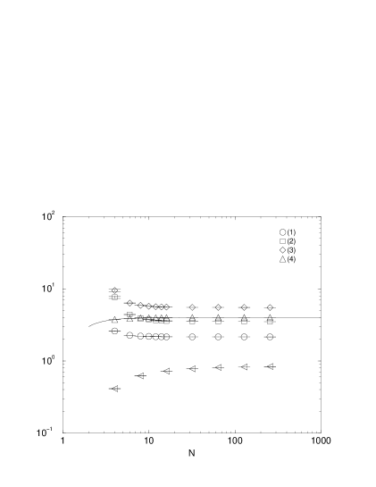
Figure 2: The quantities (1)(circles),(2)(squares),(3)(diamonds) and (4)(triangles) are plotted against $N$ for the bosonic model with $D=4$. The solid line represents the exact result (2.41) for (4). The tilted triangles are the plot of $\left\langle\Delta^{2}\right\rangle/(\sqrt{g}N^{1/4})^{2}$, which is discussed in Section 3.

In order to see the finite $N$ effects, we plot in Fig. 3 the same data against $1/N^{2}$. The data can be fitted nicely to $a_{0}+\frac{a_{1}}{N^{2}}+\frac{a_{2}}{N^{4}}$. In Section 4.2, we will see that this large $N$ behavior of the observables (1)$\sim$(4) agrees with the one given by the $1/D$ expansion.

Figure 3: The quantities (1)(circles),(2)(squares),(3)(diamonds) and (4)(triangles) are plotted against $1/N^{2}$ for the bosonic model with $D=4$. The solid line represents the exact result (2.41) for (4). The other lines represent the fits to $a_{0}+\frac{a_{1}}{N^{2}}+\frac{a_{2}}{N^{4}}$.

In Fig. 4, we plot the data for $D=10$ with $N=2\sim 32$. Here again we find that the quantities (1)$\sim$(4) are constant for $N\gtrsim 16$. We have also checked that the data can be fitted nicely to $a_{0}+\frac{a_{1}}{N^{2}}+\frac{a_{2}}{N^{4}}$.

Figure 4: The quantities (1)(circles),(2)(squares),(3)(diamonds) and (4)(triangles) are plotted against $N$ for the bosonic model with $D=10$. The solid line represents the exact result (2.41) for (4). The tilted triangles are the plot of $\left\langle\Delta^{2}\right\rangle/(\sqrt{g}N^{1/4})^{2}$, which is discussed in Section 3.

It is rather surprising that the leading large $N$ behavior shows up at about the same $N$ for $D=4$ and $D=10$. If the system were a gas model with $N$ particles in a $D$-dimensional space time, the large $N$ behavior would be expected naively to show up at such $N$ that satisfies $N^{1/D}\gg 1$. In Section 3, we define the uncertainty of the space-time coordinates and show that it is of the same order as the extent of space time, which means that the bosonic model indeed can hardly be considered as a gas model with $N$ particles in a $D$-dimensional space time.

From the results of the Monte Carlo simulation, we find that the extent of space time $R=\sqrt{\langle\frac{1}{N}\mbox{tr}(A^{2})\rangle}$ is of the order of $O(\sqrt{g}N^{1/4})$, which means that the upper bound on $R$ given in the previous sections for $D\geq 4$ is actually saturated. Due to this, the perturbative estimation of the large $N$ behavior of correlation functions given in Section 2.1.2 with the input of $R\sim O(\sqrt{g}N^{1/4})$ is valid for $D\geq 4$, which is also confirmed directly by the Monte Carlo simulation.

Figure 5: The quantities (1)(circles),(2)(squares),(3)(diamonds) and (4)(triangles) are plotted against $N$ for the bosonic model with $D=3$. The results for the $D=4$ are replotted for comparison. The solid line and the dashed line represent the exact result (2.41) for (4) for $D=3$ and $D=4$, respectively.

We have done a simulation for the $D=3$ case also, since it is rather an exceptional case from the perturbative point of view, as we remarked in Section 2.1.4. The result is shown in Fig. 5. One can see that the result is qualitatively the same as for the $D=4$ case. The fact that the upper bound $R\lesssim\sqrt{g}N^{1/3}$ is not saturated means that the perturbative arguments completely break down in the $D=3$ case due to the ultraviolet contributions. We will see in Section 4.3, however, that the $1/D$ expansion is valid even for $D=3$, which explains why the results for $D=3$ are qualitatively the same as those for $D\geq 4$.

2.3 Relation to the U(1)^D SSB of the EK model

In this section, we examine the relation of our result concerning the extent of space time to the U(1)^D SSB of the $D$-dimensional Eguchi-Kawai model.

The action of the $D$-dimensional Eguchi-Kawai model [1] is given by

$$S_{EK}=-N\beta\sum_{\mu\neq\nu=1}^{D}\mbox{tr}(U_{\mu}U_{\nu}U^{{\dagger}}_{\mu}U^{{\dagger}}_{\nu}).$$ (2.42)

This model has a U(1)^D symmetry.

$$U_{\mu}\to\mbox{e}^{i\theta_{\mu}}U_{\mu}.$$ (2.43)

In Ref. [1], it has been shown that if the U(1)^D symmetry is not spontaneously broken, the model is equivalent to an SU($N$) lattice gauge theory on an infinite lattice in the large $N$ limit, where the coupling constant $\beta$ in the action (2.42) is kept fixed.

It is found in Ref. [2] that when $D$ is larger than two, the U(1)^D symmetry is spontaneously broken in the weak coupling (large $\beta$) region. This means that we cannot study the continuum limit of the large $N$ gauge theory by the EK model when $D>2$, since we have to send $\beta$ to infinity when we take the continuum limit. Slightly modified versions of the model known as the quenched EK model [2, 4, 5] and the twisted EK model [11] have been shown to be equivalent to the SU($N$) lattice gauge theory on the infinite lattice in the large $N$ limit.

Here we note that the bosonic model is actually equivalent to the weak coupling limit of the original EK model for $D>2$. This can be seen as follows [2]. Since $U_{\mu}$ is unitary, the eigenvalues of $U_{\mu}$ are on a unit circle in the complex plane. The U(1)^D symmetry rotates all the eigenvalues by the same angle. In the weak coupling limit, namely when $\beta\rightarrow\infty$, the U(1)^D symmetry is spontaneously broken and the eigenvalues collapse to a point. Therefore, when $\beta$ is sufficiently large, the dominant configurations are given by

$$U_{\mu}\sim\mbox{e}^{i\alpha_{\mu}}\mbox{e}^{iA_{\mu}},$$ (2.44)

where $\alpha_{\mu}$ are real numbers defined modulo $2\pi$ and $A_{\mu}$ are $N\times N$ traceless hermitian matrices, whose eigenvalues are small. $\alpha_{\mu}$ take random values due to the U(1)^D symmetry. The action for $A_{\mu}$ is obtained by putting (2.44) in (2.42) and expanding it in terms of $A_{\mu}$. We obtain the following.

$$S_{EK}\sim-\frac{1}{2}N\beta\sum_{\mu\neq\nu=1}^{D}\mbox{tr}([A_{\mu},A_{\nu}]^{2})+\mbox{(higher order terms in $A$)}.$$ (2.45)

In the weak coupling limit, the higher order terms can be neglected and we arrive at the bosonic model (1.1) with $g=\frac{1}{\sqrt{2N\beta}}$.

A quantity which represents the extent of the eigenvalue distribution in the Eguchi-Kawai model can be defined by [2]

$$P=\frac{1}{2}\left\{1-\frac{1}{DN^{2}}\sum_{\mu}|\mbox{tr}~{}U_{\mu}|^{2}\right\}.$$ (2.46)

As can be seen in the above expression, $0\leq P\leq\frac{1}{2}$ for any $U_{\mu}$. $P\sim\frac{1}{2}$ when the eigenvalues are uniformly distributed, while $P\sim 0$ when the eigenvalues collapse. Thus $\langle P\rangle$ serves as an order parameter for the SSB of the U(1)^D symmetry.

Let us consider $\langle P\rangle$ in the weak coupling limit. Putting (2.44) in (2.46) and expanding it in terms of $A_{\mu}$, we obtain, to the leading order of $A_{\mu}$,

$$P\sim\frac{1}{2DN}\sum_{\mu}\mbox{tr}(A_{\mu}^{~{}2}).$$ (2.47)

Therefore $\langle P\rangle\sim\frac{1}{2D}R^{2}$, where $R$ is the extent of the eigenvalue distribution defined in the bosonic model. In Section 2.2, we have seen that $R^{2}=C(\sqrt{g}N^{1/4})^{2}$ in the large $N$ limit. This means that

$$\langle P\rangle\sim\frac{C}{2\sqrt{2}D}\frac{1}{\beta^{1/2}},$$ (2.48)

as $\beta\rightarrow\infty$. Thus our finding for the bosonic model can be interpreted in terms of the EK model as the eigenvalue distribution having a finite extent in the large $N$ limit for fixed $\beta$ in the weak coupling region. We check this explicitly by a Monte Carlo simulation in what follows.

A Monte Carlo simulation of the EK model with $D=4$ and $N=20$ has been performed in Ref. [12], where the internal energy defined by

$$E=\left\langle\frac{1}{N}\frac{1}{D(D-1)}\sum_{\mu\neq\nu}\mbox{tr}(U_{\mu}U_{\nu}U_{\mu}^{\dagger}U_{\nu}^{\dagger})\right\rangle$$ (2.49)

is measured. The asymptotic behavior of the quantity in the weak coupling limit can be obtained just in the same way as we derived (2.48). The result to the leading order of $A_{\mu}$ reads [12]

$$E \sim 1+\frac{1}{2ND(D-1)}\left\langle\sum_{\mu\neq\nu}\mbox{tr}([A_{\mu},A_{\nu}]^{2})\right\rangle$$ (2.50)

$$= 1-\frac{1}{4(D-1)}\left(1-\frac{1}{N^{2}}\right)\frac{1}{\beta},$$

where we used the exact result (2.41) in the second equality.

Figure 6: The order parameter $\langle P\rangle$ for the U(1)^D symmetry (open squares) as well as the internal energy $E$ (filled squares) is plotted against $\beta$ for the $D=4$ SU(16) Eguchi-Kawai model. The solid line and the dashed line represent the asymptotic behavior of $\langle P\rangle$ and $E$ respectively at large $\beta$ predicted by the bosonic model.

In Fig. 6, we plot the order parameter $\langle P\rangle$ as well as the internal energy $E$ for the SU(16) EK model. The solid line and the dashed line represent the asymptotic behavior at large $\beta$ for $\langle P\rangle$ (2.48) with $C=2.162(5)$ and that for $E$ (2.50), respectively, predicted by the bosonic model. The data for large $\beta$ fit nicely to the predictions. The results for the internal energy are in good agreement with the results in Ref. [12], though $N$ differs from ours slightly. We have also done simulations with $N=32$ and $N=64$ for $\beta=1.0$ and checked that both $E$ and $\langle P\rangle$ remain the same within error bars. This large $N$ behavior is just the one we expect from the large $N$ behavior of the quantities (1) and (4) in the bosonic model obtained in Section 2.2.

$\langle P\rangle$ is around 0.5 for $\beta\lesssim 0.17$ and decreases for $\beta\gtrsim 0.17$, which shows that the U(1)^D symmetry is spontaneously broken at around $\beta=\beta_{c}\sim 0.17$. At the critical point $\beta=\beta_{c}$, the internal energy is continuous but its first derivative with respect to $\beta$ seems to diverge, which suggests that the system undergoes a second order phase transition.

It is intriguing to compare the phase diagram of the EK model with that of the TEK model [11, 13]. Since the U(1)^D symmetry is not spontaneously broken in the TEK model even in the weak coupling region, the model is equivalent to the SU($N$) lattice gauge theory on the infinite lattice in the large $N$ limit throughout the whole region of $\beta$ [11]. The system undergoes a first order phase transition at $\beta\sim 0.35$. This phase transition can be considered as an artifact of the Wilson’s plaquette action, and could be avoided if one wishes, say, by introducing the adjoint term [13].

If the $\beta_{c}$, at which the SSB of the U(1)^D symmetry occurs in the EK model, were larger than 0.35, the EK model would also have undergone a first order phase transition at $\beta\sim 0.35$, but the fact is that $\beta_{c}<0.35$ and the model is not equivalent to the SU($N$) lattice gauge theory for $\beta>\beta_{c}$. Thus the first order phase transition may well be absent in the EK model.

Before ending this section, let us address the issue [10] whether the bosonic model can be used to calculate correlation functions in the large $N$ Yang-Mills theory. It is natural to think that the answer is in the negative considering the fact that the EK model is not equivalent to the large $N$ lattice gauge theory for $D>2$ due to the SSB of the U(1)^D symmetry. Let us see how this can be restated within the bosonic model.

One way to show the equivalence between the reduced model and the original model in the large $N$ limit is to confirm it to all orders of the perturbative expansion [3, 4, 5], where $\lambda_{\mu i}$ should be identified with the loop momenta and the extent of space time $R$ plays the role of the momentum cutoff. One can easily see that the coupling constant $g_{YM}$ of the corresponding Yang-Mills theory is given by

$$g_{YM}^{~{}2}=\frac{g^{2}}{R^{D}},$$ (2.51)

which can be also deduced on dimensional grounds. In order to take a nontrivial large $N$ limit, namely the ’t Hooft limit, one has to fix $g_{YM}^{~{}2}N=\lambda_{YM}$ to a constant. Since $R=C^{1/2}\sqrt{g}N^{1/4}$, where $C$ is a fixed constant determined dynamically, we obtain

$$\lambda_{YM}=C^{-\frac{D}{2}}(g^{2}N)^{1-\frac{D}{4}}.$$ (2.52)

From (2.52), we have to fix $g^{2}N$ to reproduce the ’t Hooft limit. In this limit, $R$ goes to a constant, which we denote by $\Lambda$. $\lambda_{YM}$ can then be written as

$$\lambda_{YM}=C^{-2}\Lambda^{4-D},$$ (2.53)

which means that we are not allowed to take the continuum limit $\Lambda\rightarrow\infty$ as one wishes, but the coupling constant $\lambda_{YM}$ is doomed to scale canonically with the cutoff $\Lambda$. Thus, there is no way to take a nontrivial continuum limit in the Yang-Mills theory to which the bosonic model is equivalent perturbatively. We therefore conclude that the bosonic model cannot be used to calculate correlation functions in the large $N$ Yang-Mills theory.

3 Breakdown of the classical space-time picture

As we mentioned in the Introduction, the eigenvalues of $A_{\mu}$ represent the space-time coordinates, when we interpret the IIB matrix model as a string theory formulated nonperturbatively. If $A_{\mu}$’s are mutually commutative, they can be diagonalized simultaneously and the diagonal elements after diagonalization can be regarded as the classical space-time coordinates. This must be violated more or less by $A_{\mu}$’s generated dynamically in the IIB matrix model. Therefore it makes sense to ask to what extent the classical space-time picture is broken. In order to address this issue, we define a quantity which represents the uncertainty of the space-time coordinates. We determine its large $N$ behavior for the bosonic model and show that it is of the same order as the extent of space time, which means that the classical space-time picture is maximally broken in the bosonic model.

We define such a quantity by considering an analogy to the quantum mechanics. We regard the matrices $A_{\mu}$’s as linear operators which act on a linear space, which we identify as the space of states of particles. We take an orthonormal basis $|e_{i}\rangle$ ($i=1,2,\cdots,N$) of the $N$-dimensional linear space, and identify the ket $|e_{i}\rangle$ with the state of the $i$-th particle. The space-time coordinate of the $i$-th particle can be defined by $\langle e_{i}|A_{\mu}|e_{i}\rangle$. The uncertainty $\delta(i)$ of the space-time coordinate of the $i$-th particle can be defined by

$$\delta(i)^{2}=\sum_{\mu}\left\{\langle e_{i}|A_{\mu}^{~{}2}|e_{i}\rangle-(\langle e_{i}|A_{\mu}|e_{i}\rangle)^{2}\right\}.$$ (3.1)

Note that this quantity is invariant under a Lorentz transformation and a translation : $A_{\mu}\rightarrow A_{\mu}+\alpha_{\mu}$. We take an average of $\delta(i)^{2}$ over all the $N$ particles.

$$\overline{\delta^{2}}=\frac{1}{N}\sum_{i}\delta(i)^{2}.$$ (3.2)

Note that this quantity depends on the orthonormal basis $|e_{i}\rangle$ ($i=1,2,\cdots,N$) we choose. We therefore define a quantity $\Delta$ which represents the uncertainty of the space-time coordinates for a given $A_{\mu}$ by

$$\Delta^{2} = \min_{\{|e_{i}\rangle\}}(\overline{\delta^{2}})$$ (3.3)

$$= \frac{1}{N}\mbox{tr}(A_{\mu}^{~{}2})-\max_{U\in\mbox{\scriptsize SU}(N)}\frac{1}{N}\sum_{i}\{(UA_{\mu}U^{\dagger})_{ii}\}^{2}.$$ (3.4)

Note that $\Delta$ is invariant under a gauge transformation: $A_{\mu}\rightarrow gA_{\mu}g^{\dagger}$. Note also that $\Delta=0$ if and only if $A_{\mu}$ are diagonalizable simultaneously. The classical space-time picture is good if $\Delta$ is smaller than the typical distance $\ell\sim R\cdot N^{-1/D}$ between two nearest-neighboring particles.

We calculate $\langle\Delta^{2}\rangle$ for the bosonic model by a Monte Carlo simulation. Given a configuration $A_{\mu}$, which is generated by a Monte Carlo simulation, we evaluate $\Delta^{2}$ numerically by performing the maximization of $\sum_{i}\{(UA_{\mu}U^{\dagger})_{ii}\}^{2}$ in (3.4) in the following way. We first maximize $\sum_{i}\{(UA_{\mu}U^{\dagger})_{ii}\}^{2}$ restricting the $U$ to be in one of the SU(2) subgroup of the SU($N$). Redefining the $A_{\mu}$ by the $U_{0}A_{\mu}U_{0}^{\dagger}$, where $U_{0}$ is the element of the SU(2) subgroup that gives the maximum, we do the maximization for all the $~{}_{N}\mbox{C}_{2}$ SU(2) subgroups successively. We call this as ‘one sweep’ in our maximization procedure. For $N\leq 32$, the quantity saturates up to 16 digits within 200 sweeps for $D=4$, and within 500 sweeps for $D=10$. For $D=4$, we have done the measurement with larger $N$ as well. For $N=256$, we have made 300 sweeps of the maximization, with which the saturation is achieved up to 3 digits. The result thus obtained is plotted in Figs. 2 and 4. We find that $\langle\Delta^{2}\rangle$ normalized by $(\sqrt{g}N^{1/4})^{2}$ tends to a constant for large $N$. Thus we conclude that $\sqrt{\langle\Delta^{2}\rangle}$ is of the same order as $R$.

We have seen in Section 2.2 that the $N$ at which the leading large $N$ behavior dominates does not depend much on $D$. The large $N$ behavior would show up for $N^{1/D}\gg 1$ if the system can be viewed as $N$ classical particles in a $D$-dimensional space time. Indeed our conclusion in this section means that the bosonic model can hardly be viewed as consisting of $N$ particles.

4 $1/D$ expansion of the bosonic model

4.1 The formalism

In this section, we show that the bosonic model allows a systematic $1/D$ expansion, which serves as an analytical method complementary to the Monte Carlo simulation. To all orders of the $1/D$ expansion, we determine the large $N$ behavior of correlation functions and prove the large $N$ factorization property. We also perform an explicit calculation of the quantities (1)$\sim$(4) defined in Section 2.2 up to the next-leading order and compare the results with the Monte Carlo data for various $D$, from which we conclude that the $1/D$ expansion is valid down to $D=3$.

Here we use again the adjoint notation defined through

$$A_{\mu}=\sum_{a=1}^{N^{2}-1}A_{\mu}^{~{}a}~{}t^{a},$$ (4.1)

where $t^{a}$ are the generators of SU($N$). Taking the generators $t^{a}$ to satisfy the orthonormal condition

$$\mbox{tr}(t^{a}t^{b})=\delta_{ab},$$ (4.2)

we have the following relation

$$\sum_{a}(t^{a})_{ij}(t^{a})_{kl}=\delta_{il}\delta_{jk}-\frac{1}{N}\delta_{ij}\delta_{kl}.$$ (4.3)

We first rewrite the action (1.1) for the bosonic model as

$$S = -\frac{1}{4g^{2}}\mbox{tr}([A_{\mu},A_{\nu}]^{2})$$ (4.4)

$$= -\frac{1}{4g^{2}}\lambda^{abcd}A_{\mu}^{~{}a}A_{\mu}^{~{}b}A_{\nu}^{~{}c}A_{\nu}^{~{}d},$$

where we have defined

$$\lambda^{abcd}=\frac{1}{4}\left\{\mbox{tr}([t^{a},t^{c}][t^{b},t^{d}])+(a\leftrightarrow b)+(c\leftrightarrow d)+\left(\begin{array}[]{c}a\leftrightarrow b\\ c\leftrightarrow d\end{array}\right)\right\}.$$ (4.5)

Note that the measure (1.3) can be written as $\prod_{\mu a}\mbox{d}A_{\mu}^{~{}a}$ up to an irrelevant constant factor. We introduce the auxiliary field $h_{ab}$, which is a real symmetric tensor, with the following action.

$$S[A,h] = \frac{1}{4g^{2}}\lambda^{abcd}(h_{ab}h_{cd}-A_{\mu}^{~{}a}A_{\mu}^{~{}b}h_{cd}-h_{ab}A_{\nu}^{~{}c}A_{\nu}^{~{}d})$$ (4.6)

$$= \frac{1}{4g^{2}}\lambda^{abcd}h_{ab}h_{cd}+\frac{1}{2g}K_{ab}A_{\mu}^{~{}a}A_{\mu}^{~{}b},$$ (4.7)

where we have defined the dimensionless kernel

$$K_{ab}=-\frac{1}{g}\lambda^{abcd}h_{cd}$$ (4.8)

for $A_{\mu}^{a}$. Integrating out the auxiliary field, we reproduce the original action (4.4).

Since the $A_{\mu}^{~{}a}$ is quadratic in (4.7), we can integrate it out first. The propagator for $A_{\mu}^{~{}a}$ is given by

$$\langle A_{\mu}^{~{}a}A_{\nu}^{~{}b}\rangle=g\delta_{\mu\nu}(K^{-1})_{ab}.$$ (4.9)

For example, $\langle\mbox{tr}(A^{2})\rangle$ can be expressed by the following integral.

$$\langle\mbox{tr}(A^{2})\rangle=\frac{\int\mbox{d}h_{ab}gD(K^{-1})_{aa}\mbox{e}^{-S_{\mbox{\tiny eff}}}}{\int\mbox{d}h_{ab}\mbox{e}^{-S_{\mbox{\tiny eff}}}}.$$ (4.10)

$S_{\mbox{\scriptsize eff}}$ is the effective action for $h$ defined by

$$S_{\mbox{\scriptsize eff}}=\frac{D}{2}\mbox{Tr}\ln K+\frac{1}{4g^{2}}\lambda^{abcd}h_{ab}h_{cd},$$ (4.11)

where the Tr represents a trace over the adjoint indices $a$.

By rescaling the $h$ as $\tilde{h}_{ab}=\frac{1}{g\sqrt{D}}h_{ab}$, which is now dimensionless, we can rewrite the effective action as

$$S_{\mbox{\scriptsize eff}}=\frac{D}{2}\left\{\mbox{Tr}\ln K+\frac{1}{2}\lambda^{abcd}\tilde{h}_{ab}\tilde{h}_{cd}\right\}.$$ (4.12)

Therefore, in the large $D$ limit, the integration over $\tilde{h}$ is dominated by the saddle point and one can perform a systematic $1/D$ expansion. The saddle point equation can be given as

$$(K^{-1})_{cd}\frac{\delta K_{dc}}{\delta\tilde{h}_{ab}}+\lambda^{abcd}\tilde{h}_{cd}=0.$$ (4.13)

The relevant saddle point $\tilde{h}_{ab}^{(0)}$, if we assume that it preserves the SU($N$) symmetry, should be written as $\tilde{h}_{ab}^{(0)}=v\delta_{ab}$. From the saddle point equation (4.13), we obtain $v=\frac{1}{\sqrt{2N}}$. We expand the $\tilde{h}_{ab}$ around the saddle point $\tilde{h}_{ab}^{(0)}$ as

$$\tilde{h}_{ab}=\frac{1}{\sqrt{2N}}\delta_{ab}+2\sqrt{\frac{N}{D}}\varphi_{ab},$$ (4.14)

where $\varphi_{ab}$ is real symmetric. We have put the factor $2\sqrt{\frac{N}{D}}$ in front of $\varphi_{ab}$ for later convenience. Expanding $K$ in terms of $\varphi$, we obtain

$$K_{ab}=\sqrt{2ND}(\delta_{ab}-\epsilon X_{ab}),$$ (4.15)

where $\epsilon=\sqrt{\frac{2}{D}}$ and

$$X_{ab}=\lambda^{abcd}\varphi_{cd}.$$ (4.16)

We can expand $(K^{-1})_{ab}$ and $\mbox{Tr}\ln K$ in terms of $\varphi$ in the following way.

$$(K^{-1})_{ab} = \frac{1}{\sqrt{2ND}}(\delta_{ab}+\epsilon X_{ab}+\epsilon^{2}X_{ac}X_{cd}+O(\varphi^{3})),$$ (4.17)

$$\mbox{Tr}\ln K = \mbox{const.}-\epsilon X_{aa}-\frac{1}{2}\epsilon^{2}X_{ab}X_{ba}+O(\varphi^{3}).$$ (4.18)

The effective action $S_{\mbox{\scriptsize eff}}$ can be expanded in terms of $\varphi$ as

$$S_{\mbox{\scriptsize eff}}=\frac{1}{2}T^{abcd}\varphi_{ab}\varphi_{cd}-\sum_{n=3}^{\infty}\frac{\epsilon^{n-2}}{n}\mbox{Tr}(X^{n})+\mbox{const.},$$ (4.19)

where we have defined

$$T^{abcd}=-\lambda^{abef}\lambda^{cdef}+2N\lambda^{abcd}.$$ (4.20)

The propagator of $\varphi_{ab}$ can be given by

$$\langle\varphi_{ab}\varphi_{cd}\rangle=S^{abcd},$$ (4.21)

where $S^{abcd}$ is defined by

$$T^{abpq}S^{pqcd}=S^{abpq}T^{pqcd}=I^{abcd}.$$ (4.22)

In order to obtain $S^{abcd}$ explicitly, we introduce the following quantities.

$$F^{abcd} = \frac{1}{4}(f^{abcd}+f^{bacd}+f^{abdc}+f^{badc}),$$ (4.23)

$$G^{abcd} = \frac{1}{2}(f^{acbd}+f^{adbc}),$$ (4.24)

$$H^{abcd} = \delta_{ab}\delta_{cd},$$ (4.25)

$$I^{abcd} = \frac{1}{2}(\delta_{ac}\delta_{bd}+\delta_{ad}\delta_{bc}),$$ (4.26)

where

$$f^{abcd}=\mbox{tr}(t^{a}t^{b}t^{c}t^{d}).$$ (4.27)

$\lambda^{abcd}$ and $T^{abcd}$ can be written as follows.

$$\lambda^{abcd} = 2(G^{abcd}-F^{abcd})$$ (4.28)

$$T^{abcd} = -6NF^{abcd}+4NG^{abcd}-2H^{abcd}-4I^{abcd}.$$ (4.29)

$S^{abcd}$ can be obtained as

$$S^{abcd}=\frac{1}{4(N^{2}-1)}\left\{-\frac{2}{3N}F^{abcd}+NG^{abcd}+\frac{1}{6N^{2}}H^{abcd}+I^{abcd}\right\}.$$ (4.30)

Figure 7:

Since we work with $X_{ab}$ instead of $\varphi_{ab}$ in what follows, we introduce the propagator of $X_{ab}$ given as

$$V^{abcd} \stackrel{{\scriptstyle\rm def}}{{=}} \langle X_{ab}X_{cd}\rangle$$ (4.31)

$$= \lambda^{abef}S^{efgh}\lambda^{ghcd}$$ (4.32)

$$= \frac{1}{N^{2}-1}\left\{-\frac{2}{3}NF^{abcd}+NG^{abcd}+\frac{1}{6}H^{abcd}+I^{abcd}\right\}.$$ (4.33)

Let us represent $V^{abcd}$ by the four-point vertex, as is shown in Fig. 7. Then we can calculate $\langle\mbox{tr}(A^{2})\rangle$ by evaluating the diagrams depicted in Fig. 8.

Figure 8:

The result is given as follows.

$$\langle\mbox{tr}(A^{2})\rangle=gD\frac{1}{\sqrt{2ND}}\left\{(N^{2}-1)+\epsilon^{2}\left(V^{abab}+V^{aabc}V^{bddc}\right)+O(\epsilon^{4})\right\},$$ (4.34)

where each term corresponds to the diagrams (a), (b) and (c) in Fig. 8, respectively. By noting that $V^{abcc}=-\frac{1}{2}\delta_{ab}$ and $V^{abab}=\frac{1}{6}(7N^{2}-1)$, we obtain the result for the quantity (1) defined in Section 2.2 as

$$(1) \stackrel{{\scriptstyle\rm def}}{{=}} \left\langle\frac{1}{N}\mbox{tr}(A^{2})\right\rangle\times\left(\sqrt{g}N^{1/4}\right)^{-2}$$ (4.35)

$$= \sqrt{\frac{D}{2}}\left\{\left(1-\frac{1}{N^{2}}\right)+\frac{1}{D}\left(\frac{7}{6}-\frac{1}{6N^{2}}\right)+O\left(\frac{1}{D^{2}}\right)\right\}.$$

Similarly, we can calculate $\langle\mbox{tr}((A_{\mu}A_{\nu})^{2})\rangle$ as follows.

$$\langle\mbox{tr}((A_{\mu}A_{\nu})^{2})\rangle$$ (4.36)

$$= G^{abcd}\langle A_{\mu}^{~{}a}A_{\mu}^{~{}b}A_{\nu}^{~{}c}A_{\nu}^{~{}d}\rangle$$

$$= g^{2}G^{abcd}\{D^{2}\langle(K^{-1})_{ab}(K^{-1})_{cd}\rangle+2D\langle(K^{-1})_{ac}(K^{-1})_{bd}\rangle\}$$

$$= g^{2}\frac{1}{2ND}[D^{2}\{G^{aabb}+\epsilon^{2}(G^{abcd}V^{abcd}+2G^{aabc}V^{bddc}+2G^{abcc}V^{abde}V^{dffe})\}$$

$$~{}~{}~{}~{}~{}~{}~{}~{}~{}~{}+2DG^{abab}+O(1)].$$

$\langle\mbox{tr}((A^{2})^{2})\rangle$ can be calculated by replacing $G$ by $F$ in the above expressions. We obtain the following final results for the quantities (2) and (3).

$$(2) \stackrel{{\scriptstyle\rm def}}{{=}} \left\langle\frac{1}{N}\mbox{tr}((A_{\mu}A_{\nu})^{2})\right\rangle\times\left(\sqrt{g}N^{1/4}\right)^{-4}$$ (4.37)

$$= D\left\{-\frac{1}{2N^{2}}\left(1-\frac{1}{N^{2}}\right)+\frac{1}{D}\left(\frac{3}{2}-\frac{5}{2N^{2}}+\frac{1}{N^{4}}\right)+O\left(\frac{1}{D^{2}}\right)\right\},$$

$$(3) \stackrel{{\scriptstyle\rm def}}{{=}} \left\langle\frac{1}{N}\mbox{tr}((A^{2})^{2})\right\rangle\times\left(\sqrt{g}N^{1/4}\right)^{-4}$$ (4.38)

$$= D\left\{\frac{1}{2}\left(1-\frac{1}{N^{2}}\right)^{2}+\frac{1}{D}\left(\frac{3}{2}-\frac{5}{2N^{2}}+\frac{1}{N^{4}}\right)+O\left(\frac{1}{D^{2}}\right)\right\}.$$

Note that the above results are consistent with the exact result (2.41) for $\langle\frac{1}{N}\mbox{tr}(F^{2})\rangle$.

4.2 Large $N$ behavior and factorization

We estimate the order in $N$ of correlation functions to all orders of the $1/D$ expansion and further prove the large $N$ factorization property.

Let us first consider $\langle\frac{1}{N}\mbox{tr}(A^{2})\rangle$ as an example. The diagrams we encounter up to the next-leading order in the $1/D$ expansion are shown in Fig. 8. We estimate the order in $N$ of each diagram we encounter at each order of the $1/D$ expansion. We start by replacing the $V^{abcd}$ by the r.h.s. of (4.33). Each $V$-vertex should be replaced by either of the $F$-, $G$-,$H$- and $I$-vertices with the factor $\frac{1}{N}$ for the first two, and with the factor $\frac{1}{N^{2}}$ for the last two due to the coefficients in (4.33). We denote the number of $F$- and $G$-vertices by $V_{1}$ and the number of $H$- and $I$-vertices by $V_{2}$ in the diagram after this replacement. The diagram has an overall factor $\left(\frac{1}{N}\right)^{V_{1}}\left(\frac{1}{N^{2}}\right)^{V_{2}}$.

The next task is to replace the $F$-,$G$-,$H$- and $I$-vertices by their definitions (4.23)$\sim$(4.26). Let us introduce the diagrammatic representation for $\mbox{tr}(t^{a}t^{b}\cdots t^{c})$ as in Fig. 9.

Figure 9:

Fig. 10 shows an example of what we get from the diagram (c) of Fig. 8. The symbols $F$ and $H$ in the l.h.s. of Fig. 10 represent that the $V$-vertices in the diagram (c) of Fig. 8 have been replaced by $F$- and $H$- vertices respectively.

Figure 10:

In general, we obtain diagrams composed of $V_{1}$ blobs connected by $L$ lines with additional $\ell$ loops which are not connected to any of the blobs. Reflecting the fact that each blob has four legs, we have

$$4V_{1}=2L.$$ (4.39)

Let us denote by $C$ the number of connected parts in the diagram excluding the additional $\ell$ loops. For the diagram shown in the r.h.s. of Fig. 10, we have $C=1$ and $\ell=1$. Since the number of connected parts has a chance to increase from its initial value ‘1’ by the use of $H$- and $I$- vertices, we have

$$C+\ell=1+j,$$ (4.40)

where $j=0,1,\cdots,V_{2}$. The $\ell$ loops give a factor of $(N^{2})^{\ell}$.

In order to read off the order in $N$ of the diagram, it is convenient to switch at this stage to the double-line notation. The $\mbox{tr}(t^{a}t^{b}\cdots t^{c})$ should be represented as in Fig. 11.

Figure 11:

Due to the relation (4.3), we have the diagrammatic rule depicted in Fig. 12

Figure 12:

for the contraction of the adjoint indices. In order to see the leading large $N$ behavior, it suffices to consider only the first term. Fig. 13 shows the diagram in the double-line notation which gives the leading large $N$ contribution to the diagram on the r.h.s. in Fig. 10.

Figure 13:

If we denote by $F$ the number of index loops excluding those coming from the $\ell$ additional loops, we have the following relation

$$F+V_{1}-L=2C-2h,$$ (4.41)

where $h$ is the number of handles necessary to write the diagram without crossings of the double lines.

The order of magnitude of the contribution to $\langle\frac{1}{N}\mbox{tr}(A^{2})\rangle$ from the diagram is given by

$$\frac{1}{N}\frac{g}{\sqrt{N}}\left(\frac{1}{N}\right)^{V_{1}}\left(\frac{1}{N^{2}}\right)^{V_{2}}(N^{2})^{\ell}N^{F}$$ (4.42)

$$= g\sqrt{N}\cdot(N^{2})^{(j-V_{2})-h},$$

where we have used (4.39),(4.40) and (4.41). Therefore the leading term is $O(g\sqrt{N})$, which is obtained for $j=V_{2}$ and $h=0$.

So far, we have been concentrating on the leading large $N$ behavior. Let us next consider sub-leading terms. Note first that the sub-leading terms from (4.42) are given in terms of a $1/N^{2}$ expansion. The effect of the second term in Fig. 12 is a factor either of $O(1)$ or of $O(\frac{1}{N^{2}})$ for each replacement of the first term by the second term. Also the prefactor $\frac{1}{N^{2}-1}$ of (4.33) can be expanded in terms of $1/N^{2}$, which may give extra $O(\frac{1}{N^{2}})$ factors, as well. Thus we have shown that the subleading terms appear as a $1/N^{2}$ expansion.

Generalization of the above argument to the quantity written as

$$\left\langle\frac{1}{N}\mbox{tr}(\underbrace{A\cdots A}_{p_{1}})\frac{1}{N}\mbox{tr}(\underbrace{A\cdots A}_{p_{2}})\cdots\frac{1}{N}\mbox{tr}(\underbrace{A\cdots A}_{p_{Q}})\right\rangle$$ (4.43)

is straightforward. (4.39), (4.40) and (4.41) should be replaced by

$$4V_{1}+P = 2L,$$ (4.44)

$$C+\ell = q+j,$$ (4.45)

$$F+(V_{1}+Q)-L = 2C-2h,$$ (4.46)

where $P=\sum_{i=1}^{Q}p_{i}$ and $q=1,2,\cdots,Q$. $q$ is the number of connected parts before replacing the $V$-vertices by either of $F$-,$G$-,$H$- and $I$-vertices. Then the order of magnitude of the quantity (4.43) is given by

$$\left(\frac{1}{N}\right)^{Q}\left(\frac{g}{\sqrt{N}}\right)^{P/2}\left(\frac{1}{N}\right)^{V_{1}}\left(\frac{1}{N^{2}}\right)^{V_{2}}(N^{2})^{\ell}N^{F}$$ (4.47)

$$= (\sqrt{g}N^{1/4})^{P}N^{2\{(q-Q)+(j-V_{2})-h\}},$$

where we have used (4.44), (4.45) and (4.46). Therefore, we have the maximum order $(\sqrt{g}N^{1/4})^{P}$ when $q=Q$, $j=V_{2}$ and $h=0$ and the sub-leading terms appear as a $1/N^{2}$ expansion.

Thus we have shown, to all orders of the $1/D$ expansion, that if we define

$${\cal O}=\frac{1}{N}\mbox{tr}(\underbrace{A\cdots A}_{p})\times(\sqrt{g}N^{1/4})^{-p},$$ (4.48)

correlation functions of ${\cal O}$’s such as $\langle{\cal O}_{1}{\cal O}_{2}\cdots{\cal O}_{n}\rangle$ have finite large $N$ limits. Note that this large $N$ behavior is the same as the one obtained by the perturbative argument in Section 2.1.2 with the input of $R\sim\sqrt{g}N^{1/4}$. The fact that the large $N$ behavior of the correlation functions does not depend on the order of the $1/D$ expansion is consistent with the fact that the perturbative argument is independent of $D$ except for $D=3$. We have also shown that the subleading large $N$ behavior of the correlation functions can be given by a $1/N^{2}$ expansion, which is clearly seen by the Monte Carlo simulation in Section 2.2. Moreover, the fact that the leading large $N$ contribution to (4.43) comes solely from the diagrams with $q=Q$ as is seen from (4.47) means that we have the factorization property :

$$\langle{\cal O}_{1}{\cal O}_{2}\cdots{\cal O}_{n}\rangle=\langle{\cal O}_{1}\rangle\langle{\cal O}_{2}\rangle\cdots\langle{\cal O}_{n}\rangle+O\left(\frac{1}{N^{2}}\right)$$ (4.49)

in the large $N$ limit.

The factorization can be generalized to the case when ${\cal O}$’s are Wilson loop operators such as

$${\cal O}=\frac{1}{N}{\cal P}\exp(i\int\mbox{d}\sigma k_{\mu}(\sigma)A_{\mu}).$$ (4.50)

We here consider $k_{\mu}(\sigma)$ to be written as

$$k_{\mu}(\sigma)=\frac{1}{\sqrt{g}N^{1/4}}f_{\mu}(\sigma),$$ (4.51)

where $f_{\mu}(\sigma)$ is independent of $g$ and $N$. Then the above quantity can be expanded in terms of $f$ as

$${\cal O} = \frac{1}{N}{\cal P}\exp(i\int\mbox{d}\sigma k_{\mu}(\sigma)A_{\mu})$$ (4.52)

$$= \sum_{n=0}^{\infty}i^{n}\int_{0}^{1}\mbox{d}\sigma_{1}\int_{\sigma_{1}}^{1}\mbox{d}\sigma_{2}\cdots\int_{\sigma_{n-1}}^{1}\mbox{d}\sigma_{n}f_{\mu_{1}}(\sigma_{1})f_{\mu_{2}}(\sigma_{2})\cdots f_{\mu_{n}}(\sigma_{n})$$

$$~{}~{}~{}\frac{1}{N}\mbox{tr}(A_{\mu_{n}}\cdots A_{\mu_{2}}A_{\mu_{1}})\times(\sqrt{g}N^{1/4})^{-n}.$$

Therefore the factorization property is satisfied by the Wilson operators considered above as well. This is in contrast to the situation seen in the double scaling limit of the 2D Eguchi-Kawai model, studied as a toy model of the IIB matrix model [15].

4.3 Comparison of the $1/D$ expansion with numerical data

Figure 14: The quantities (1)(circles),(2)(squares),(3)(diamonds) and (4)(triangles) extrapolated to $N=\infty$ and normalized by the leading asymptotic behavior in the large $D$ limit are plotted against $1/D$ for the bosonic model. The solid line represents the exact result (2.41) for (4) and the other lines represent the fits to $1+b_{1}/D+b_{2}/D^{2}+b_{3}/D^{3}+b_{4}/D^{4}$ with the input of the $1/D$ expansion up to the next-leading terms.

In order to confirm that the $1/D$ expansion developed in the previous sections is valid for studying the large $N$ limit of the model for finite $D$, we perform Monte Carlo simulations for various $D$ and examine the $D$ dependence of the quantities (1)$\sim$(4) defined in Section 2.2. Extrapolation to $N=\infty$ has been done by the fit to $a_{0}+a_{1}/N^{2}$ with $N=16$, 32, 64, 128, 256 for $D=3$, 4, with $N=16$, 32, 64 for $D=6$, 8, and with $N=16$, $32$ for $D=10,12,14,20$. In order to compare the data with the results of the $1/D$ expansion (4.35), (4.37) and (4.38), where we put $N=\infty$, we normalize the Monte Carlo data by the leading asymptotic behavior in the large $D$ limit. For (2), since the leading term in $1/D$ vanishes in the $N\rightarrow\infty$ limit, we normalize the data by the next-leading term. In Fig. 14, we plot the results against $1/D$. We fit the data to $1+b_{1}/D+b_{2}/D^{2}+b_{3}/D^{3}+b_{4}/D^{4}$, except for (4), which is known exactly. For (1) and (3), we use the values of $b_{1}$ predicted by the next-leading term. We find that the data are nicely fitted.

This result suggests that we do not have a phase transition at some intermediate value of $D$ and that the $1/D$ expansion is valid for finite $D$ down to $D=3$.

5 No SSB of Lorentz invariance

In this section, we address the issue of the SSB of the Lorentz invariance in large $N$ reduced models. This is of paramount importance in the IIB matrix model, since if the space time is to be four-dimensional at all, the 10D Lorentz invariance of the model must be spontaneously broken.

Let us define an order parameter for the SSB of the Lorentz invariance. We first note that the extent of the eigenvalue distribution in the direction $n_{\mu}$, where $n_{\mu}$ is a $D$-dimensional unit vector, can be given by the square root of

$$I(n) = \frac{1}{N}\mbox{tr}~{}(n\cdot A)^{2}$$ (5.1)

$$= I_{\mu\nu}n_{\mu}n_{\nu},$$ (5.2)

where $I_{\mu\nu}$ is a $D\times D$ real symmetric matrix defined by

$$I_{\mu\nu}=\frac{1}{N}\mbox{tr}(A_{\mu}A_{\nu}).$$ (5.3)

The eigenvalues of $I_{\mu\nu}$ are real positive. The SSB of the Lorentz invariance can be probed by the variation of the eigenvalues, which is given by

$$J = \frac{1}{D}I_{\mu\nu}I_{\mu\nu}-\left(\frac{1}{D}I_{\mu\mu}\right)^{2}$$ (5.4)

$$= \frac{1}{D}\left\{\frac{1}{N}\mbox{tr}(A_{\mu}A_{\nu})\right\}^{2}-\frac{1}{D^{2}}\left\{\frac{1}{N}\mbox{tr}(A^{2})\right\}^{2}.$$ (5.5)

If $\langle J\rangle/R^{4}$ is nonzero in the large $N$ limit, where $R\sim\sqrt{g}N^{1/4}$ is the (averaged) extent of space time, the Lorentz invariance is spontaneously broken. Therefore, $\langle J\rangle/(\sqrt{g}N^{1/4})^{4}$ can be considered as an order parameter for the SSB of the Lorentz invariance.

In Fig. 15 we plot $\frac{\langle J\rangle}{(\sqrt{g}N^{1/4})^{4}}$ against $N$ for $D=4,6,8$ and $10$. We see that the order parameter vanishes in the large $N$ limit, which means that the Lorentz invariance is not spontaneously broken.

Figure 15: The order parameter for the SSB of the Lorentz invariance $\langle J\rangle/(\sqrt{g}N^{1/4})^{4}$ is plotted against $N$ for $D=4,6,8$ and $10$. The solid line represents the leading large $N$ behavior for $D=\infty$ and the other lines represent the fits of the data to the $1/N^{2}$ behavior predicted by (4.49).

This result can be also confirmed by the $1/D$ expansion. By using the $1/D$ expansion, we can prove a relation

$$\langle\mbox{tr}(A_{\mu}A_{\nu})\rangle=\frac{1}{D}\delta_{\mu\nu}\langle\mbox{tr}(A^{2})\rangle,$$ (5.6)

which already suggests the absence of an SSB of the Lorentz invariance. In fact, this relation combined with the relation

$$\left\langle\frac{1}{N}\mbox{tr}(A_{\mu}A_{\nu})\frac{1}{N}\mbox{tr}(A_{\lambda}A_{\rho})\right\rangle\times\left(\sqrt{g}N^{1/4}\right)^{-4}$$ (5.7)

$$= \left\langle\frac{1}{N}\mbox{tr}(A_{\mu}A_{\nu})\right\rangle\left\langle\frac{1}{N}\mbox{tr}(A_{\lambda}A_{\rho})\right\rangle\times\left(\sqrt{g}N^{1/4}\right)^{-4}+O\left(\frac{1}{N^{2}}\right),$$

due to the large $N$ factorization property (4.49), which can be also shown by the $1/D$ expansion, leads to $\frac{\langle J\rangle}{(\sqrt{g}N^{1/4})^{4}}=O(\frac{1}{N^{2}})$ in the large $N$ limit. Indeed the large $N$ behavior of the order parameter obtained by the Monte Carlo simulation can be nicely fitted to $1/N^{2}$.

We have also calculated the order parameter by the $1/D$ expansion explicitly. The result is given as

$$\frac{\langle J\rangle}{(\sqrt{g}N^{1/4})^{4}}=\frac{1}{2N^{2}}\left\{1+\frac{17}{3D}+O\left(\frac{1}{D^{2}}\right)\right\}+O\left(\frac{1}{N^{4}}\right).$$ (5.8)

The leading large $N$ behavior for $D=\infty$ is plotted in Fig. 15 for comparison.

6 Summary and Discussion

In this paper, we studied the reduced model of bosonic Yang-Mills theory with special attention to dynamical aspects related to the eigenvalues of the $N\times N$ matrices, which are regarded as the space-time coordinates in the IIB matrix model. We found that the bosonic model allows a systematic $1/D$ expansion, which indeed revealed many interesting dynamical properties of the model. One should note again that the parameter $g$ of the model, which corresponds to the coupling constant before being reduced, is merely a scale parameter which can be scaled out if one wishes by an appropriate redefinition of the dynamical variables $A_{\mu}$. Thus, unlike in ordinary gauge theories, we have neither a weak coupling expansion nor a strong coupling expansion. $1/D$ is the only parameter which allows a systematic expansion of the model. We confirmed that the $1/D$ expansion is indeed valid for all $D\geq 3$.

To all orders of the expansion, we estimated the large $N$ behavior of correlation functions, which agrees with the one determined by the Monte Carlo simulation. Above all, the extent of space time, which is defined by $R=\sqrt{\langle\frac{1}{N}\mbox{tr}(A^{2})\rangle}$, was found to behave as $R\sim\sqrt{g}N^{1/4}$ in the large $N$ limit. For $D\geq 4$, the above result turned out to saturate the upper bound given by perturbative arguments, which fact makes the perturbative estimation of the large $N$ behavior of correlation functions valid. We also showed that the large $N$ behavior of the extent of space time is consistent with the SSB of the U(1)^D symmetry in the weak coupling region of the Eguchi-Kawai model.

The fact that we could obtain an upper bound on $R$ through a perturbative evaluation of the effective action has an important implication. It means that if we look at the effective action for the eigenvalues $\lambda_{\mu i}$ obtained perturbatively, it has nonnegligible contributions when a pair of $\lambda_{i}$’s which are assigned to adjacent index loops on a Feynman diagram (e.g., Fig. 1) are separated widely in the $D$-dimensional space time. This gives an obstacle to identifying the Feynman diagrams with smooth worldsheets of strings, which means that the bosonic model cannot be interpreted as a string theory. We expect that the situation changes drastically in the supersymmetric case.

We defined a quantity representing the uncertainty of the space-time coordinates and showed that it is of the same order as the extent of space time, which means that a classical space-time picture is maximally broken. To all orders of the $1/D$ expansion, we found that correlation functions are given by an expansion in terms of $1/N^{2}$. This makes, e.g., $N=16$ sufficiently large to probe the large $N$ behavior of the model even for large $D$. We pointed out that this is related to the maximal breakdown of the classical space-time picture.

The absence of an SSB of the Lorentz invariance was shown both by the Monte Carlo simulation and by the $1/D$ expansion.

All the above issues we addressed for the bosonic model should be addressed for the IIB matrix model as well. The results must reveal all the dynamical properties of the model related to the space-time structure and the worldsheet picture. We expect that the supersymmetry plays an essential role. We hope our findings for the bosonic model provide a helpful comparison when we investigate the supersymmetric case including the IIB matrix model.

Appendix: The algorithm for the Monte Carlo simulation

In this appendix, we explain the algorithm we use for the Monte Carlo simulation of the bosonic model with the action

$$S=-\frac{1}{2}\beta\sum_{\mu<\nu}\mbox{tr}([A_{\mu},A_{\nu}]^{2}),$$ (A.1)

where $\beta=\frac{1}{g^{2}}$. Since $\mu\neq\nu$, the action is quadratic with respect to each component, which means that we can update each component by generating gaussian variables using the heat bath algorithm.

We first note that the trace can be written as

$$\mbox{tr}([A_{\mu},A_{\nu}]^{2})=2(A_{\mu})_{ij}(A_{\nu})_{jk}(A_{\mu})_{kl}(A_{\nu})_{li}-2(A_{\mu})_{ij}(A_{\nu}^{~{}2})_{jk}(A_{\mu})_{ki}.$$ (A.2)

Suppose we want to update $A_{\mu}$. In the first term, all the $N^{2}$ components are coupled, while in the second term, only the components which include at least one common index are coupled.

In order to simplify the algorithm, we employ the following trick. We first rewrite the action as

$$S=-\frac{1}{2}\beta\sum_{\mu<\nu}\mbox{tr}(\{A_{\mu},A_{\nu}\}^{2})+2\beta\sum_{\mu<\nu}\mbox{tr}(A_{\mu}^{~{}2}A_{\nu}^{~{}2}).$$ (A.3)

Here we introduce the auxiliary field $Q_{\mu\nu}$ ($1\leq\mu<\nu\leq D$), which is $~{}_{D}\mbox{C}_{2}$ $N\times N$ hermitian matrices, with the following action

$$S^{\prime}=\frac{1}{2}\beta\sum_{\mu<\nu}\mbox{tr}(Q_{\mu\nu}^{~{}2}-2Q_{\mu\nu}G_{\mu\nu})+2\beta\sum_{\mu<\nu}\mbox{tr}(A_{\mu}^{~{}2}A_{\nu}^{~{}2}),$$ (A.4)

where $G_{\mu\nu}$ is an hermitian matrix defined by

$$G_{\mu\nu}=\{A_{\mu},A_{\nu}\}.$$ (A.5)

Integrating out the auxiliary field $Q_{\mu\nu}$, one reproduces the original action (A.3).

Note that the simultaneous update of each of $(Q_{\mu\nu})_{ij}$ can be done easily by generating Gaussian variables. As for the update of $A_{\mu}$, note that only the components which include at least one common index are coupled due to the second term of (A.4). The $N$ diagonal components $(A_{\mu})_{ii}$ ($i=1,\cdots,N$) for each $\mu$ can be updated simultaneously. The $\frac{N}{2}$ off-diagonal components $(A_{\mu})_{n_{1}n_{2}}$, $(A_{\mu})_{n_{3}n_{4}}$, …, $(A_{\mu})_{n_{N-1}n_{N}}$, where $n_{1},n_{2},\cdots,n_{N}$ are different indices, can be updated simultaneously for each $\mu$.

References

- [1] T. Eguchi and H. Kawai, Phys. Rev. Lett. 48 (1982) 1063.
- [2] G. Bhanot, U. Heller and H. Neuberger, Phys. Lett. 113B (1982) 47.
- [3] G. Parisi, Phys. Lett. 112B (1982) 463.
- [4] D. Gross and Y. Kitazawa, Nucl. Phys. B206 (1982) 440.
- [5] S. Das and S. Wadia, Phys. Lett. 117B (1982) 228.
- [6] T. Banks, W. Fischler, S.H. Shenker and L. Susskind, Phys. Rev. D55 (1997) 5112, hep-th/9610043.
- [7] N. Ishibashi, H. Kawai, Y. Kitazawa and A. Tsuchiya, Nucl. Phys. B498 (1997) 467, hep-th/9612115.
- [8] M. Fukuma, H. Kawai, Y. Kitazawa and A. Tsuchiya, Nucl. Phys. B510 (1998) 158, hep-th/9705128.
- [9] H. Aoki, S. Iso, H. Kawai, Y. Kitazawa and T. Tada, Prog. Theor. Phys. 99 (1998) 713, hep-th/9802085.
- [10] W. Krauth and M. Staudacher, Phys. Lett. B435 (1998) 350, hep-th/9804119.
- [11] A. Gonzalez-Arroyo and M. Okawa, Phys. Rev. D27 (1983) 2397.
- [12] M. Okawa, Phys. Rev. Lett. D49 (1982) 705.
- [13] J. Nishimura, Mod. Phys. Lett. A11 (1996) 3049, hep-lat/9608119.
- [14] T. Yoneya, p. 419 in “Wandering in the Fields”, eds. K. Kawarabayashi and A. Ukawa (World Scientific, 1987); p. 23 in “Quantum String Theory”, eds. N. Kawamoto and T. Kugo (Springer, 1988); Mod. Phys. Lett. A4 (1989) 1587.
- [15] T. Nakajima and J. Nishimura, Nucl. Phys. B528 (1998) 355, hep-th/9802082.