Abstract. We calculate the Hausdorff dimension, $d_{H}$, and the correlation function exponent, $\eta$, for polymerized two dimensional quantum gravity models. If the non-polymerized model has correlation function exponent $\eta_{0}>3$ then $d_{H}=\gamma^{-1}$ where $\gamma$ is the susceptibility exponent. This suggests that these models may be in the same universality class as certain non-generic branched polymer models.

The idea of polymerization was first introduced in the context of matrix models [1, 2, 3] and then later generalized to an arbitrary random surface theory (ie model of discretized two dimensional quantum gravity) by Durhuus [4]. The basic idea is that the random surface (universe) can have other random surfaces (baby universes) attached with the minimal possible contact (this is defined more carefully below). Depending upon the fugacity for these contact terms the system can exist in one of three phases; at low fugacity there is a single random surface with few outgrowths attached, at high fugacity there are many outgrowths and the system is a generic branched polymer, and at an intermediate point there is a branched polymer structure in which each node is itself a critical surface. This point is the polymerized model and has been studied in a number of papers [5, 6, 7, 8]. The polymerized models have the interesting feature that their susceptibility exponent is positive but less than the generic branched polymer value $1/2$. In this letter we compute the Hausdorff dimension of these polymerized models.

In general we define the grand canonical partition function for an ensemble of graphs ${\mathcal{G}}$ by

$${\mathcal{Z}}(\mu)=\sum_{{\mathrm{G}}\in{\mathcal{G}}}e^{-\mu{|{\mathrm{G}}|}}w_{{\mathrm{G}}}$$ (1)

where ${|{\mathrm{G}}|}$ denotes the number of points in G, and $w_{{\mathrm{G}}}$ the weight for the graph G (for an introduction to this material see for example [9]). We will assume throughout that graphs are defined with one marked point. The sum in (1) is convergent for $\mu>\mu_{c}$ and as $\mu\to\mu_{c}$ we expect

$${\mathcal{Z}}(\mu)\simeq R_{1}-R_{2}(\mu-\mu_{c})^{1-\gamma}$$ (2)

where $R_{1,2}$ are regular functions of $\mu$. In addition we define the susceptibility

$$\chi(\mu)=-\frac{\partial{\mathcal{Z}}(\mu)}{\partial\mu}\sim A-B(\mu-\mu_{c})^{-\gamma}$$ (3)

where $A$ and $B$ are constants.

Now consider an ensemble of graphs ${\mathcal{G}}$ constructed from a base graph ensemble ${\mathcal{G}}_{0}$ and a “baby” graph ensemble ${\mathcal{G}}_{1}$; all the graphs in ${\mathcal{G}}_{0,1}$ are assumed to have weight $w_{{\mathrm{G}}}=1$. As shown in fig.1, baby graphs are attached to the base graph with a fugacity $\rho$ by identifying their marked point with a point in the base graph (this is slightly different from the usual construction but more convenient for our purpose). For a given base graph points such as ‘a’, to which no baby is attached, contribute a factor 1 to $w_{{\mathrm{G}}}$, whereas points ‘b’ contribute a factor $\rho e^{\mu}{\mathcal{Z}}_{1}(\mu)$ once all baby graphs have been summed over. The extra factor of $e^{\mu}$ multiplying $Z_{1}(\mu)$ arises because we are identifying points in the base and baby graphs. This reduces the total number of points in the product graph by one in comparison to the base and baby taken separately. Summing over all possible ways of attaching the babies to the base graph we obtain

$${\mathcal{Z}}(\mu) = \sum_{{\mathrm{G}}\in{\mathcal{G}}_{0}}e^{-\mu{|{\mathrm{G}}|}}\left(1+\rho e^{\mu}{\mathcal{Z}}_{1}(\mu)\right)^{{|{\mathrm{G}}|}}$$ (4)

$$= {\mathcal{Z}}_{0}({\bar{\mu}})$$ (5)

where

$${\bar{\mu}}=\mu-\log\left(1+\rho e^{\mu}{\mathcal{Z}}_{1}(\mu)\right).$$ (6)

The structure defined in (5) and (6) is identical to that derived in [4]. Throughout this letter we will denote the value of ${\bar{\mu}}$ at which ${\mathcal{Z}}_{0}({\bar{\mu}})$ is non-analytic by ${\bar{\mu}}_{0}$.

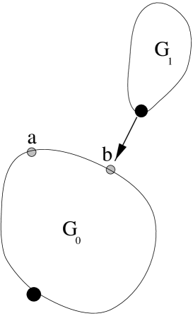
Figure 1: Attaching a baby ${{\mathrm{G}}}_{1}\in{{\mathcal{G}}}_{1}$ to the base graph ${{\mathrm{G}}}_{0}\in{{\mathcal{G}}}_{0}$. The solid circles denote the marked points on the two graphs and the shaded circles points on the base graph.

Now consider the two-point function

$${\mathcal{H}}(R,\mu)=\sum_{{\mathrm{G}}\in{\mathcal{G}}}e^{-\mu{|{\mathrm{G}}|}}\sum_{i\in{\mathrm{G}}}\delta(d_{{\mathrm{G}}}(i)-R)$$ (7)

where $d_{{\mathrm{G}}}(i)$ is the geodesic distance of the point $i$ from the marked point on G. Note that

$$\sum_{R=0}^{\infty}{\mathcal{H}}(R,\mu)=-\frac{\partial{\mathcal{Z}}(\mu)}{\partial\mu}=\chi(\mu).$$ (8)

We expect that ${\mathcal{H}}$ has the asymptotic behaviour [10, 11]

$${\mathcal{H}}(R,\mu)\sim e^{-m(\mu)R}, \quad m(\mu)R>>1$$

$$\sim R^{1-\eta}, \quad m(\mu)^{-1}>>R>>1.$$ (9)

As $\mu\to\mu_{c}$, the mass gap vanishes as

$$m(\mu)\sim(\mu-\mu_{c})^{\nu}$$ (10)

where the correlation length exponent is related to the Hausdorff dimension $d_{H}$ by $d_{H}\nu=1$. ${\mathcal{H}}$ is related by discrete Laplace transformation to the canonical ensemble quantity $n(R,N)$; this is the expectation on graphs with a fixed number of vertices, $N$, of the number of vertices a geodesic distance $R$ from the fixed point. It is expected that

$$n(R,N)\sim R^{d_{h}-1}f\left(\frac{R^{d_{H}}}{N}\right)$$ (11)

where $f(x)$ is $O(1)$ at small $x$ and vanishes at large $x$ [11]. The Hausdorff dimension $d_{h}$ is not necessarily the same as $d_{H}$ (for example on multi-critical branched polymers they are different [12, 13]).

If G is constructed from a base graph with babies there are two sorts of contribution to (7). The first is where the point $i$ lies in the base graph. The second is where the point $i$ lies in a baby ${\mathrm{G}}_{1}$ which is attached to the base graph ${\mathrm{G}}_{0}$ at $k$ say; in this case we have

$$d_{{\mathrm{G}}}(i)=d_{{\mathrm{G}}_{0}}(k)+d_{{\mathrm{G}}_{1}}(i)$$ (12)

and of course G must contain at least one baby. Attaching babies to points in the base graph as described above (fig.1) we then find that

$${\mathcal{H}}(R,\mu) = \sum_{{\mathrm{G}}\in{\mathcal{G}}_{0}}e^{-\mu{|{\mathrm{G}}|}}\left(1+\rho e^{\mu}{\mathcal{Z}}_{1}(\mu)\right)^{{|{\mathrm{G}}|}}\sum_{i\in{\mathrm{G}}}\delta(d_{{\mathrm{G}}}(i)-R)$$ (13)

$$+\sum_{r=1}^{R}\sum_{{\mathrm{G}}\in{\mathcal{G}}_{0}}e^{-\mu{|{\mathrm{G}}|}}\left(1+\rho e^{\mu}{\mathcal{Z}}_{1}(\mu)\right)^{{|{\mathrm{G}}|}-1}\sum_{k\in{\mathrm{G}}_{0}}\delta(d_{{\mathrm{G}}}(k)-R+r)$$

$$\qquad\times\rho e^{\mu}\sum_{{\mathrm{G}}^{\prime}\in{\mathcal{G}}_{1}}e^{-\mu{|{\mathrm{G}}^{\prime}|}}\sum_{i\in{\mathrm{G}}^{\prime}}\delta(d_{{\mathrm{G}}^{\prime}}(i)-r)$$

$$= {\mathcal{H}}_{0}(R,{\bar{\mu}})+\sum_{r=1}^{R}\frac{{\mathcal{H}}_{0}(R-r,{\bar{\mu}})\rho e^{\mu}{\mathcal{H}}_{1}(r,\mu)}{1+\rho e^{\mu}{\mathcal{Z}}_{1}(\mu)}.$$

It is straightforward to check that this expression satisfies (8).

From the point of view of quantum gravity we are interested in the case where the ensemble ${\mathcal{G}}_{1}$ from which the babies are drawn is the same as the full ensemble ${\mathcal{G}}$; this means that we set ${\mathcal{Z}}_{1}(\mu)={\mathcal{Z}}(\mu)$, and ${\mathcal{H}}_{1}(r,\mu)={\mathcal{H}}(r,\mu)$ in (5), (6) and (13). Together with the assumption that the susceptibility exponent of the ${\mathcal{G}}_{0}$ ensemble satisfies $\gamma_{0}<0$, this defines the polymerized quantum gravity models [4]. We then obtain from (6) the useful result that

$$1+\rho e^{\mu}{\mathcal{Z}}(\mu)=\left(1-\rho e^{\bar{\mu}}{\mathcal{Z}}_{0}({\bar{\mu}})\right)^{-1}.$$ (14)

To analyze the critical exponents of the polymerized theory we start by recalling the calculation of $\gamma$ [4]. By differentiating (5) we obtain

$$\chi(\mu)=\frac{\chi_{0}({\bar{\mu}})\left(1-\rho e^{\bar{\mu}}{\mathcal{Z}}_{0}({\bar{\mu}})\right)}{1-\rho e^{\bar{\mu}}\chi_{0}({\bar{\mu}})}.$$ (15)

We can identify three regimes.
i) When $\rho$ is small enough the first singularity encountered on the right hand side of (15) as $\mu$ decreases is in $\chi_{0}({\bar{\mu}})$ at ${\bar{\mu}}={\bar{\mu}}_{0}$ (note that since $\gamma_{0}<0$, $\chi_{0}({\bar{\mu}}_{0})$ is finite). From (6) we have that as $\mu\to\mu_{c}$

$${\bar{\mu}}-{\bar{\mu}}_{c}=\mu-\mu_{c}-\log\left(1-C(\mu-\mu_{c})^{(1-\gamma)}\right)$$ (16)

where $C$ is a constant. Because $\chi(\mu)$ is not divergent, $\gamma<0$ and therefore ${\bar{\mu}}-{\bar{\mu}}_{c}\sim\mu-\mu_{c}$ and hence, using (3), we have $\gamma=\gamma_{0}$.
ii) When $\rho$ is very large the denominator in (15) will vanish at a value of $\mu$ such that ${\bar{\mu}}>{\bar{\mu}}_{0}$, and $\chi_{0}({\bar{\mu}})$ is therefore still analytic, so we obtain

$$\chi(\mu)\sim\frac{1}{{\bar{\mu}}-{\bar{\mu}}_{c}}.$$ (17)

Now $\chi(\mu)$ is divergent so $\gamma>0$ and hence from (16) we obtain

$${\bar{\mu}}-{\bar{\mu}}_{c}\sim(\mu-\mu_{c})^{(1-\gamma)}$$ (18)

so that

$$\chi(\mu)\sim\frac{1}{(\mu-\mu_{c})^{(1-\gamma)}}$$ (19)

and hence, using the definition (3), we find that $\gamma=1/2$ which is the standard branched polymer exponent.
iii) At some critical value $\rho=\rho_{c}$ the susceptibility $\chi_{0}({\bar{\mu}})$ will be non-analytic and the denominator in (15) will vanish at the same value of $\mu$. In this case we find

$$\chi(\mu)\sim\frac{1}{({\bar{\mu}}-{\bar{\mu}}_{c})^{-\gamma_{0}}}.$$ (20)

Again using (18) we get

$$\chi(\mu)\sim\frac{1}{(\mu-\mu_{c})^{-\gamma_{0}(1-\gamma)}}$$ (21)

and hence

$$\gamma=\frac{-\gamma_{0}}{1-\gamma_{0}}.$$ (22)

This result applies provided $\gamma_{0}>-1$. If $\gamma_{0}<-1$ then the denominator in (20) is linear in ${\bar{\mu}}-{\bar{\mu}}_{c}$ and we obtain $\gamma=1/2$.

Now we can study ${\mathcal{H}}(R,\mu)$ in these three regimes. Since (13) is a convolution it is convenient to introduce

$${\widetilde{{\mathcal{H}}}}(\omega,\mu)=\sum_{r=0}^{\infty}{\mathcal{H}}(r,\mu)e^{-\omega r}$$ (23)

and similarly for ${\mathcal{H}}_{0}(r,\mu)$. Then from (13) we obtain

$${\widetilde{{\mathcal{H}}}}(\omega,\mu)=\frac{\left(1-\rho e^{\bar{\mu}}{\mathcal{Z}}_{0}({\bar{\mu}})\right){\widetilde{{\mathcal{H}}}}_{0}(\omega,{\bar{\mu}})}{1-\rho e^{\bar{\mu}}{\widetilde{{\mathcal{H}}}}_{0}(\omega,{\bar{\mu}})}$$ (24)

which reproduces (15) if we set $\omega=0$. From the general behaviour (9) we expect that the singularities in $\omega$ of ${\widetilde{{\mathcal{H}}}}(\omega,\mu)$ will lie on the negative real axis. The dominant physical behaviour is given by the nearest singularity to the origin (or more precisely by the singularities that converge onto the origin as $\mu\to\mu_{c}$). To establish $d_{H}$ it is sufficient to establish the behaviour of the location of this singularity, $\omega_{0}$, because by (9) we expect $\omega_{0}=-m\sim-(\mu-\mu_{c})^{\nu}$.

In regime i) ${\widetilde{{\mathcal{H}}}}_{0}(\omega,{\bar{\mu}})$ has a singularity at $\omega\sim-({\bar{\mu}}-{\bar{\mu}}_{0})^{\nu_{0}}$. However, the denominator of (24) takes the same value at $\omega=0$ as does the denominator of (15) and is therefore finite and positive; thus ${\widetilde{{\mathcal{H}}}}(\omega,\mu)$ is singular at the same value of $\omega$ as ${\widetilde{{\mathcal{H}}}}_{0}(\omega,{\bar{\mu}})$ and $d_{H}=d_{H_{0}}$. The $\eta$ exponent is found by considering (24) at $\mu=\mu_{c}$; from (9) we get

$${\widetilde{{\mathcal{H}}}}_{0}(\omega,{\bar{\mu}}_{c}) \sim \sum_{r=1}^{\infty}r^{1-\eta_{0}}e^{-\omega r}$$ (25)

$$= {\widetilde{{\mathcal{H}}}}_{0}(0,{\bar{\mu}}_{c})-b\omega+\ldots+c\omega^{\eta_{0}-2}+\ldots,$$

where $b$ and $c$ are constants, and a similar expression for ${\widetilde{{\mathcal{H}}}}(\omega,\mu_{c})$; we see that $\eta$ controls the leading non-analyticity in $\omega$. Substituting (25) in (24) we see that $\eta=\eta_{0}$. We might also conclude that $d_{h}=d_{h_{0}}$ on the grounds that ${\widetilde{{\mathcal{H}}}}(\omega,\mu)$ has the same leading singularity structure as ${\widetilde{{\mathcal{H}}}}_{0}(\omega,{\bar{\mu}})$ but with a multiplicatively modified residue; however this is not a complete proof since the inverse Laplace transform required to extract $n(R,N)$ from ${\widetilde{{\mathcal{H}}}}(\omega,\mu)$ is rather delicate.

In regime ii) we know that the denominator in (24) vanishes at $\omega=0$ when ${\bar{\mu}}>{\bar{\mu}}_{0}$ and ${\widetilde{{\mathcal{H}}}}_{0}(\omega,{\bar{\mu}})$ is analytic in the vicinity of $\omega=0$. Thus we can write

$$\left({\widetilde{{\mathcal{H}}}}_{0}(\omega,{\bar{\mu}})\right)^{-1}=\left({\widetilde{{\mathcal{H}}}}_{0}(0,{\bar{\mu}})\right)^{-1}\left(1+a\omega+\dots\right)$$ (26)

where $a$ is finite and the series is convergent; substituting this in (24) we get

$${\widetilde{{\mathcal{H}}}}(\omega,\mu)=\frac{\left(1-\rho e^{\bar{\mu}}{\mathcal{Z}}_{0}({\bar{\mu}})\right){\widetilde{{\mathcal{H}}}}_{0}(0,{\bar{\mu}})}{1+a\omega-\rho e^{\bar{\mu}}{\widetilde{{\mathcal{H}}}}_{0}(0,{\bar{\mu}})}$$ (27)

so there is a simple pole at

$$\omega\sim-({\bar{\mu}}-{\bar{\mu}}_{c})\sim-\sqrt{\mu-\mu_{c}}.$$ (28)

${\widetilde{{\mathcal{H}}}}(\omega,\mu)$ thus consists of a simple pole plus a regular function of $\omega$. The long distance behaviour is determined entirely by the simple pole so we have pure generic branched polymer behaviour for which $d_{H}=2$, $d_{h}=2$, and $\eta=1$ [12].

At $\rho=\rho_{c}$, in regime iii), the singularity in ${\widetilde{{\mathcal{H}}}}_{0}(\omega,{\bar{\mu}})$ and the zero of the denominator in (24) coincide when $\mu=\mu_{c}$. The location of the zero is given by

$${\widetilde{{\mathcal{H}}}}_{0}(\omega_{0},{\bar{\mu}})=\frac{1}{\rho e^{\bar{\mu}}}.$$ (29)

Now we exploit the fact that ${\widetilde{{\mathcal{H}}}}_{0}(\omega,{\bar{\mu}})$ is an analytic function of $\omega$ when ${|\omega|}<<({\bar{\mu}}-{\bar{\mu}}_{c})^{\nu_{0}}$ (this is because its first singularity occurs at $\omega\sim-({\bar{\mu}}-{\bar{\mu}}_{c})^{\nu_{0}}$). So, assuming that $\omega_{0}$ lies in the region where ${\widetilde{{\mathcal{H}}}}_{0}(\omega,{\bar{\mu}})$ is analytic, and expanding (29) we obtain

$${\widetilde{{\mathcal{H}}}}_{0}(0,{\bar{\mu}})+\sum_{n=1}^{\infty}\frac{\omega_{0}^{n}}{n!}\frac{\partial^{n}{\widetilde{{\mathcal{H}}}}_{0}(\omega,{\bar{\mu}})}{\partial\omega^{n}}\Bigg{|}_{\omega=0}=\frac{1}{\rho e^{\bar{\mu}}}.$$ (30)

From the definition (23) we have that

$$\frac{\partial^{n}{\widetilde{{\mathcal{H}}}}_{0}(\omega,{\bar{\mu}})}{\partial\omega^{n}}\Bigg{|}_{\omega=0}=\sum_{r=0}^{\infty}(-r)^{n}{\mathcal{H}}_{0}(r,{\bar{\mu}}).$$ (31)

We can use the asymptotic behaviour (9) to deduce the leading behaviour of these moments of ${\mathcal{H}}_{0}(r,{\bar{\mu}})$. For example we can compute the moments of the trial function

$${\mathcal{H}}_{trial}(R,\mu)= m(\mu)^{\eta-1}e^{1-m(\mu)R}, \quad m(\mu)R\geq 1$$

$$= R^{1-\eta}, \quad m(\mu)^{-1}>R\geq 1$$ (32)

which has the correct asymptotic behaviour and is continuous; it is easy to check that, assuming Fisher scaling, the zeroth moment has the same form as the susceptibility. For the higher moments we find

$$\frac{\partial^{n}{\widetilde{{\mathcal{H}}}}_{0}(\omega,{\bar{\mu}})}{\partial\omega^{n}}\Bigg{|}_{\omega=0}\sim a_{n},\hfil \quad n<\eta_{0}-2$$

$$\sim a_{n}\log({\bar{\mu}}-{\bar{\mu}}_{c}), \quad n=\eta_{0}-2$$

$$\sim a_{n}({\bar{\mu}}-{\bar{\mu}}_{c})^{-\gamma_{0}-n\nu_{0}}, \quad n>\eta_{0}-2$$ (33)

where the $a_{n}$ are constants. In the pure gravity case $\eta_{0}=4$ and so (30) gives

$$\omega_{0}a_{1}+\omega_{0}^{2}a_{2}\log({\bar{\mu}}-{\bar{\mu}}_{c})+\omega_{0}^{3}a_{3}({\bar{\mu}}-{\bar{\mu}}_{c})^{-\gamma_{0}-3\nu_{0}}+\ldots\sim-({\bar{\mu}}-{\bar{\mu}}_{c})^{-\gamma_{0}}$$ (34)

and hence

$$\omega_{0}\sim-({\bar{\mu}}-{\bar{\mu}}_{c})^{-\gamma_{0}}.$$ (35)

Note that (35) is consistent with the assumption that ${|\omega_{0}|}<<({\bar{\mu}}-{\bar{\mu}}_{c})^{\nu_{0}}$. It is easy to check that provided $\eta_{0}>3$ this procedure is consistent and that (35) is the correct solution. It follows immediately that

$$\nu=-\frac{\gamma_{0}}{1-\gamma_{0}}=\gamma$$ (36)

and therefore that

$$d_{H}=\frac{1}{\gamma}.$$ (37)

If $\eta_{0}\leq 3$ then $\nu_{0}\geq-\gamma_{0}$ and hence the dominant singularities in (30) must occur at $\omega_{0}\sim-({\bar{\mu}}-{\bar{\mu}}_{c})^{\nu_{0}}$ and so

$$d_{H}=\frac{1-\gamma_{0}}{\nu_{0}}.$$ (38)

As usual the $\eta$ exponent is found by considering (24) at $\mu=\mu_{c}$. Using (25) we see that if $\eta_{0}>3$ the term linear in $\omega$ dominates as $\omega\to 0$ and, substituting into (24), we get

$${\widetilde{{\mathcal{H}}}}(\omega,\mu_{c})\sim\frac{1}{\omega}$$ (39)

and hence that $\eta=1$; thus the Fisher scaling relation $\nu(2-\eta)=\gamma$ is satisfied. On the other hand if $\eta_{0}\leq 3$ then the non-analytic term in (25) dominates and we get

$${\widetilde{{\mathcal{H}}}}(\omega,\mu_{c})\sim\frac{1}{\omega^{\eta_{0}-2}}$$ (40)

and hence that $\eta=4-\eta_{0}$; again it is easy to check that Fisher scaling is obeyed.

There are at present only two cases for which we know the Hausdorff dimension of the base graph. The first is that of pure (ie $c=0$) quantum gravity [14, 10] for which $d_{H_{0}}=4$, $\eta_{0}=4$, $\gamma_{0}=-1/2$; at $\rho=\rho_{c}$ the polymerized model has $\gamma=1/3$ [4, 5] and, by our results, $d_{H}=3$ and $\eta=1$. In fact these results for a polymerized system with pure gravity base graphs have been obtained before under the assumption that the distance inside the base graph can be ignored [8]. The authors argued that the approximation was a good one on the grounds that, although the base graphs are critical, the average number of vertices in them is actually rather small. Our exact results show that their conclusion is in fact correct, and the distance in the base graphs does not affect the Hausdorff dimension. The second case is $c=-2$ quantum gravity for which $\gamma_{0}=-1$ and there is overwhelming evidence that $d_{H_{0}}=(3+\sqrt{17})/2\approx 3.562$ so that, by Fisher scaling, $\eta_{0}\approx 5.562$. At the polymerized critical point we get $\gamma=1/2$, $d_{H}=2$ and $\eta=1$ which is the same as in the branched polymer phase.

It is interesting that, at least in the case $\eta_{0}>3$, the known exponents at the polymerized critical point coincide with those of the continuously critical branched polymers studied in [15, 16]. It is easy to show, using the standard calculation of ${\mathcal{H}}$ for branched polymers that, provided only $\gamma>0$, a branched polymer has $d_{H}=1/\gamma$, $\eta=1$, $d_{h}=2$, just as for the case of multi-critical branched polymers. The multi-critical branched polymers have $\gamma>1/2$ whereas the continuously critical branched polymers can have $\gamma<1/2$ which is what happens at the polymerized critical point. Of course we have not determined $d_{h}$ or the spectral dimension $d_{s}$ for the polymerized critical point but it is at least plausible that it does indeed fall in the same universality class as the continuously critical branched polymers. This is precisely because of the argument given above; namely that the average number of vertices in a base graph is rather small.

References

[1]S. R. Das, A. Dhar, A. M. Sengupta and S. R. Wadia,
Mod. Phys. Lett. A5 (1990) 1041.
[2]L. Alvarez-Gaume, J. L. F. Barbon, and C. Crnkovic, Nucl. Phys.
B 394 (1993) 383.
[3]G. P. Korchemsky, Phys. Lett. B 296 (1992) 323;
Mod. Phys. Lett. A7 (1992) 3081.
[4]B. Durhuus, Nucl. Phys. B 426 (1994) 203.
[5]J. Ambjørn, B. Durhuus and T. Jonsson, Mod. Phys. Lett. A9
(1994)
1221.
[6]I. R. Klebanov, Phys. Rev. D51 (1995) 1836;
I. R. Klebanov and A. Hashimoto, Nucl. Phys. B434 (1995) 264.
[7] T. Jonsson and J.F.Wheater, Phys. Lett. B 345 (1995) 227.
[8]M.G.Harris and J.Ambjørn, Nucl. Phys. B 474 [FS]
(1996) 575.
[9]J. Ambjørn, B. Durhuus and T. Jonsson, Quantum Geometry,
Cambridge Monographs on Mathematical Physics, Cambridge 1997.
[10] J.Ambjørn and Y.Watabiki, Nucl. Phys. B445 (1995) 129.
[11] J.Ambjørn, J.Jurkiewicz and Y.Watabiki, Nucl. Phys. B454
(1995) 313.
[12]J.Ambjørn, B.Durhuus and T.Jonsson, Phys. Lett. B244
(1990) 403.
[13] J.Ambjørn et al, Nucl. Phys. B511 (1998) 673-710.
[14] H.Kawai, N.Kawamoto, T.Mogami and Y.Watabiki,
Phys. Lett. B306 (1993) 19; Y.Watabiki, Nucl. Phys. B441 (1995) 119.
[15]P. Bialas and Z. Burda, Phys. Lett. B 384 (1996) 75.
[16]J.D. Correia and J.F. Wheater, Phys. Lett. B422 (1998) 76.