1. New Uncertainty Principles in String Theory

A long-standing problem in string theory is to determine the structure of spacetime at very short distance scales, typically at lengths smaller than the finite intrinsic length of the strings. One of the first analytical approaches to this problem was to study the effects of high-energy string scattering amplitudes on the accuracy with which one can measure position and momentum [2]. This implies the conventional string-modified Heisenberg uncertainty principle

$$\Delta x~{}{>\!\!\!\!\!^{\,}_{\sim}}~{}\frac{\hbar}{\Delta p}+{\cal O}(\ell_{s}^{2})\,\Delta p+\dots$$ (1.1)

The modifications to the usual phase space uncertainty relation in (1.1) come from stringy corrections which are due to the finite minimum length $\ell_{s}$ of the string. In fact, minimizing the right-hand side of (1.1) shows that the string length scale gives an absolute minimum lower bound $\Delta x\geq{\cal O}(\ell_{s})$ on the measurability of distances in spacetime. This result means that, if one uses only string states as probes of short-distance structure, the conventional ideas of general relativity break down at distances smaller than $\ell_{s}$.

However, until very recently there has been no systematic derivation of (1.1) based on some set of fundamental principles. The appearence of new solitonic structures in string theory, which incorporate defects in spacetime, suggest the possibility of using such objects as probes of short-distance structure. These non-perturbative objects are known as D-branes and can be analytically described beyond the conventional string worldsheet approach. In many instances however, such as the cases that will be studied in the following, a perturbative string loop-expansion approach is still sufficient. As we will discuss in this paper, such an approach leads to new forms of uncertainty relations, in addition to (1.1), which are attributed to the recoil of the spacetime defects in the process of the scattering of string matter off the D-brane solitons. In the case of multi-brane systems, this leads to a non-commutative spacetime structure at very short distances.

In this paper we will give an exposition of these results, based mostly on the articles [3]–[6]. We will begin with a brief review of soliton structures in string theory, emphasizing the worldsheet $\sigma$-model approach to $T$-duality and Dirichlet branes. We will then describe how to view spacetime coordinates and momenta in this framework as $\sigma$-model coupling constants, such that the genus expansion leads to a canonical phase space quantization. We then specialize to the case of a system of multi-D-particles and show how one passes from Lie algebraic to spacetime non-commutativity. In this way the quantum spacetime which follows from the many-body D-particle dynamics is induced directly by the quantum string theory itself. The important aspects of the construction are a logarithmic conformal field theory formalism for the relevant recoil operators, an effective target space Lagrangian for the $\sigma$-model couplings which is described by non-abelian Born-Infeld theory, and the interpretation of the target space time as the Liouville mode of the underlying two-dimensional quantum gravity. We will show how this formalism leads to new uncertainty principles in D-brane quantum gravity. We conclude with some general remarks and outlook on the nature of time in D-brane quantum gravity, including possible experimental tests of spacetime non-commutativity from $\gamma$-ray burst observations, neutral kaon physics, and atom interferometry measurements.

Quantization of Collective Coordinates: The Basic Idea

It is worthwhile to give a quick overview of the formalism which will follow. To use D-branes as probes of the short distance properties of spacetime, we shall view the collective coordinates and momenta of D-particles as a set of $\sigma$-model couplings $\{g^{I}\}$ (this includes the case of multi-D0-brane configurations which inherently contain non-commutative structures). It follows from the Coleman approach to probabilistic couplings via two-dimensional quantum gravity wormholes [7], that the genus expansion of the worldsheet theory will lead to a quantization of the couplings $\{g^{I}\}$ [8].

The quantum field theory is described by the fixed-genus Euclidean path integral

$${\cal Z}_{\rm QFT}[\{g^{I}\}]=\int D\Phi~{}{\rm e}^{-{\cal L}_{\rm QFT}[\Phi;\{g^{I}\}]}~{}~{}~{}~{}~{}~{},~{}~{}~{}~{}~{}~{}{\cal L}_{\rm QFT}[\Phi;\{g^{I}\}]={\cal L}_{*}[\Phi]+\int_{\Sigma}d^{2}z~{}g^{I}O_{I}[\Phi]$$ (1.2)

where $\Phi$ denotes a collection of fields defined on a Riemann surface $\Sigma$. The action ${\cal L}_{*}[\Phi]$ defines a conformal field theory and $O_{I}[\Phi]$ are a set of local deformation vertex operators. The sum over all topologies of the two-dimensional quantum field theory (1.2) can be evaluated exactly in the dilute wormhole gas approximation (fig. 1) and it induces statistical fluctuations $\Delta g^{I}$ of the $\sigma$-model couplings,

$$\sum_{\rm genera}{\cal Z}_{\rm QFT}[\{g^{I}\}]\simeq\int D\alpha_{I}~{}{\cal P}[\{\alpha_{I}\}]\int D\Phi~{}{\rm e}^{-{\cal L}_{\rm QFT}[\Phi;\{g^{I}+\Delta g^{I}(\alpha)\}]}$$ (1.3)

where the fields $\alpha_{I}$ are wormhole parameters. For a dilute gas, the wormhole probability distribution function is given by

$${\cal P}[\{\alpha_{I}\}]={\cal N}\exp-\frac{1}{2\Gamma^{2}}\,\alpha_{I}\,{\cal G}^{IJ}\,\alpha_{J}$$ (1.4)

where $\Gamma$ is the width of the distribution and ${\cal G}^{IJ}$ is an appropriate metric on the moduli space of coupling constants $\{g^{I}\}$. This promotes the couplings $g^{I}$ to quantum operators $\widehat{g}^{I}=g^{I}+\Delta g^{I}$ on target space.

Figure 1: Resummation of the genus expansion in the pinched approximation. The solid circles are worldsheet discs (or spheres) and the thin lines are strips attached to them with infinitesimal pinching size $\delta$. Each strip corresponds to an insertion of a bilocal operator on the worldsheet.

Let us now specialize to the case of a system of $N$ non-relativistic heavy D-particles. In this case, the couplings $\{g^{I}\}$ are given by the set $\{Y_{ab}^{i}(X^{0}),P_{j}^{cd}(X^{0})\}$, where $Y$ are the collective coordinates of the D-particles and $P$ are their collective momenta. The indices $i,j$ label the directions in spacetime while $a,b,c,d=1,\dots,N$ label the $U(N)$ isospin gauge symmetry present in any multi-brane system. The field $X^{0}$ is the worldsheet temporal embedding coordinate and the momenta are given by $P_{i}^{ab}=M_{s}U_{i}^{ab}$, where

$$M_{s}=\frac{1}{g_{s}\ell_{s}}$$ (1.5)

is the mass of a D-particle, with $g_{s}$ the string coupling constant. According to the above general prescription, the multi-brane dynamics will induce position-momentum (or phase space), space-space, and space–time indeterminancies as follows. From the associated wormhole distribution (1.4) there follows a set of position uncertainties $\Delta Y^{i}_{ab}$ corresponding to the effective widths $\Gamma^{2}/G_{IJ}$, where $\Gamma$ is proportional to the string coupling $g_{s}$ and $G_{IJ}=\langle V_{I}V_{J}\rangle$ is the Zamolodchikov metric [9] with $\{V_{I}\}$ the set of local vertex operators associated with the D-particle couplings $\{g^{I}\}$. The momentum uncertainties $\Delta P^{ab}_{j}$ arise upon canonical quantization in the moduli space 𝕄 of $\sigma$-model couplings $\{g^{I}\}$ which leads to the quantum commutator

$$\left[\!\left[\widehat{Y}^{i}_{ab},\widehat{P}_{j}^{cd}\right]\!\right]=i\,\hbar_{{\hbox{\mybbs M}}}\,\delta_{j}^{i}\,\delta_{a}^{c}\,\delta_{b}^{d}~{}~{}~{}~{}~{}~{},~{}~{}~{}~{}~{}~{}\widehat{P}^{i}_{ab}=-i\,\hbar_{{\hbox{\mybbs M}}}\,\frac{\delta}{\delta Y^{i}_{ab}}$$ (1.6)

where the effective Planck constant $\hbar_{{\hbox{\mybbs M}}}$ of 𝕄 is of order $g_{s}$. Furthermore, the target space time $T$ in the “physical” frame depends on the positions and momenta of the D-particles and therefore becomes a target space operator $\widehat{T}$ upon summation over all worldsheet topologies. From this we will derive a space–time uncertainty relation of the form [10] $\Delta Y^{i}_{ab}\Delta T~{}{>\!\!\!\!\!^{\,}_{\sim}}~{}{\cal O}(g_{s}\ell_{s}^{2})$ which will imply, in particular, that extremely heavy D-particles can probe very small distances.

2. String Solitons and Non-abelian D-particle Dynamics

Short-distance Spacetime Structure

The discovery [11, 12] of new solitonic structures in superstring theory have dramatically changed our understanding of target space structure. These new non-perturbative objects are known as Dirichlet-branes and they can be seen to arise from the implementation of $T$-duality as a canonical transformation in the path integral [13, 14] for the usual open superstring with free endpoints. The latter object is described by imposing Neumann boundary conditions on the embedding fields $X^{M}$, $M=0,1,\dots,9$, of the string worldsheet $\Sigma$, which we assume has the topology of a disc. At the circular boundary of $\Sigma$ the fields are constant along the normal directions, $\partial_{\rm n}X^{M}=0$, and are allowed to vary as arbitrary functions $X^{M}(s)$ on $\partial\Sigma$. Here $\partial_{\rm n}$ is the normal derivative to the boundary $\partial\Sigma$ in $\Sigma$. A $T$-duality transformation $X\to\tilde{X}$, defined on the worldsheet by $\partial_{\alpha}X^{M}=\epsilon^{\alpha\beta}\partial_{\beta}\tilde{X}^{M}$, maps the Neumann boundary conditions into the Dirichlet boundary conditions $\partial_{\rm t}\tilde{X}^{M}=0$, or equivalently $\tilde{X}^{M}|_{\partial\Sigma}=Y^{M}$, where $\partial_{\rm t}$ is the derivative tangent to $\partial\Sigma$. Now the fields are fixed at the specified values $Y^{M}$ on $\partial\Sigma$ but can vary in the normal directions. If the $T$-duality mapping is applied to $9-p$ spatial directions, then the Dirichlet conditions define a hypersurface in 10-dimensional spacetime. The hypersurface is embedded into target space from an effective $p+1$ dimensional worldvolume in which the embedding fields $X^{M}$ are allowed to vary freely. These objects are known as D$p$-branes. They are solitons of the open superstring theory and supersymmetry guarantees their stability. They have a BPS mass given by (1.5) and are characterized as being topological defects which are fixed in the $9-p$ spacetime directions. Open string excitations can attach themselves to the D-brane domain walls.

In this paper we shall specialize to the case of D0-branes, or D-particles. In this case the set of string embedding fields can be written as $X^{M}=(X^{0},X^{i})$, where $X^{0}$ is the worldline time coordinate, which satisfies Neumann boundary conditions, and $X^{i}$, $i=1,\dots,9$, are the coordinates of the D-particle which obey Dirichlet boundary conditions. The dynamics of these excitations can be described by deforming the usual free string $\sigma$-model action $S_{0}[X]$ by a worldsheet boundary vertex operator [11]

$${\cal S}_{\rm C}=S_{0}[X]-\frac{1}{\ell_{s}^{2}}\oint_{\partial\Sigma}ds~{}Y_{i}(X^{0})\,\partial_{\rm n}X^{i}(s)~{}~{}~{}~{}~{}~{};~{}~{}~{}~{}~{}~{}S_{0}[X]=\frac{1}{2\ell_{s}^{2}}\int_{\Sigma}d^{2}z~{}\partial X^{M}\,\bar{\partial}X^{N}\,\eta_{MN}$$ (2.1)

where $\eta_{MN}$ is a (critical) flat Minkowski spacetime metric. The non-relativistic motion of heavy D-particles can be described by the Galilean-boosted configurations $Y^{i}(X^{0})=Y^{i}+U^{i}X^{0}$ where $U^{i}$ is the non-relativistic velocity of the branes.

The interesting situation arises when one considers a configuration of $N$ D-branes (fig. 2). The multiple D-brane assembly leads to a non-commutative structure at very short distances in the spacetime. The situation is actually quite simple. Consider a system of $N$ parallel D-branes. When the separation between branes is of a sub-Planckian distance scale, the solitons can interact with each other via the exchange of open strings. It is this property of D-brane dynamics that makes them good probes of the short-distance structure of spacetime and it implies that spacetime at very small distance scales is described by some sort of non-commutative geometry. A tractable limit of this situation is the case of overlapping branes or infinitesimal separations. More complicated situations can also arise, for instance when the branes interact via the exchange of other D-branes, in addition to their string interactions. One would then need to employ a formalism for intersecting D-brane configurations. In the following we will concentrate on the simpler situation of only open string excitations between the D-branes.

Figure 2: Emergence of the enhanced $U(N)$ gauge symmetry for bound states of $N$ parallel D-branes (planes). An oriented fundamental string (wavy lines) can start and end either at the same or different D-brane, giving $N^{2}$ massless vector states in the limit of coinciding branes. These states form a representation of $U(N)$.

Low-energy Effective Field Theories

To understand why a non-commutative structure is implied at very short distance scales, one needs to examine the effective field theory description for $N$ parallel D-branes. In the multi-D-particle case, the assembly is described by a set of $N\times N$ Hermitian matrices $Y^{i}_{ab}$, $i=1,\dots,9$, in the adjoint representation of the unitary group $U(N)$ which are obtained as the remnant fields from the dimensional reduction of 10-dimensional maximally supersymmetric $U(N)$ Yang-Mills theory to the worldlines of the D-particles [15]. The reduced Yang-Mills potential

$$V_{0}[Y]=\frac{1}{\ell_{s}^{4}}\frac{1}{4g_{s}}\sum_{i,j=1}^{9}\mbox{tr}\left[Y^{i},Y^{j}\right]^{2}$$ (2.2)

then governs the dynamics of the branes, where tr denotes the trace in the fundamental representation of $U(N)$. There are two limiting regimes of this theory. In the weak-coupling limit $g_{s}\to 0$, the branes are very far apart and do not interact with each other. The potential (2.2) is minimized by those matrix-valued configurations which satisfy $[Y^{i},Y^{j}]=0$, $\forall i,j$. These solutions correspond to states of maximal supersymmetry. In this case the generic $U(N)$ gauge symmetry of the Yang-Mills theory is broken down to $U(1)^{N}$, i.e. there is one $U(1)$ gauge field on each D-brane. Moreover, the matrix fields can be simultaneously diagonalized by a gauge transformation to give $Y^{i}={\rm diag}\{y_{(a)}^{i}\}_{a=1,\dots,N}$, where the eigenvalues $y_{(a)}^{i}$ represent the coordinates of each D-particle. Now consider the opposite case where the branes are almost on top of each other. Since the energy of a fundamental string which stretches between two different branes is $\frac{1}{2\ell_{s}}|\vec{y}_{(a)}-\vec{y}_{(b)}|$, it follows that in this case more massless vector states appear in the spectrum of the $U(N)$ gauge theory. Now the configurations of the Yang-Mills potential (2.2) satisfy $[Y^{i},Y^{j}]\neq 0$ for $i\neq j$ and correspond to states of broken supersymmetry which must be incorporated into the quantum gauge theory. Thus the limit of coinciding branes restores the full $U(N)$ gauge symmetry and leads to a Lie algebraic non-commutativity in the spacetime coordinates $Y^{i}_{ab}$. The components with $a\neq b$ are to be interpreted as the coordinates of the short open string degrees of freedom stretched between the branes, so that the D-brane coordinates are viewed as adjoint Higgs fields in this picture. These ideas are depicted schematically in fig. 2.

In the following we shall be interested in establishing the manner in which this Lie algebraic non-commutativity implies a genuine quantum spacetime non-commutativity. For this, we consider an alternative description to the Yang-Mills matrix quantum mechanics which is given by a non-local deformation of a free worldsheet $\sigma$-model. In the simplest case of non-relativistic motion, it follows from the BPS mass formula (1.5) that the limit of heavy D-particles is equivalent to taking $g_{s}\ll 1$. This is precisely the regime in which worldsheet perturbation theory can be trusted. The partition function for the uniform motion of the multi-D0-brane system in the $T$-dual Neumann picture is defined as the expectation value of a path-ordered Wilson loop operator along the worldsheet boundary in the free $\sigma$-model,

$$Z_{N}[Y]=\int DX~{}{\rm e}^{-S_{0}[X]}~{}\mbox{tr}\,{\rm P}\,\exp\left(ig_{s}\oint_{\partial\Sigma}A_{M}(X^{0}(s))~{}dX^{M}(s)\right)$$ (2.3)

where the field $A$ is an $N\times N$ Hermitian matrix in the adjoint representation of $U(N)$ with $A^{M}=(A^{0},-\frac{1}{\ell_{s}^{2}}Y^{i})$ the components of the $U(N)$ gauge potential dimensionally reduced to the worldline of the D-particles.

However, the model (2.3) on its own is a bit too naive and needs to be supplemented with some auxilliary prescriptions. There are problems with summing over worldsheet genera in the Dirichlet picture, which could be related to the breaking of the $T$-duality symmetry from an anomaly in the non-abelian case [16, 17]. Modular logarithmic divergences appear in matter field amplitudes when the string propagator $L_{0}$ is computed with Dirichlet boundary conditions. Consider a string matter field polarization tensor $V$ in the D-brane background at the level of an annular topology (fig. 3). Corresponding to a string state of conformal weight $\Delta$, the string propagator contains a modular parameter integration of the form $\int\frac{dq}{q}~{}q^{\Delta}$. In the pinched annulus limit, with infinitesimal pinching size $\delta$, the states of zero conformal dimension $\Delta=0$ therefore yield logarithmic divergences of the form $\log\delta$.

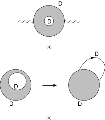
Figure 3: (a) World-sheet annulus diagram for the leading quantum correction to the propagation of a string state $V$ (wavy lines) in a D-brane background, and (b) the pinched annulus configuration which is the dominant divergent contribution to the quantum recoil.

These modular divergences are cancelled by adding logarithmic recoil operators [18] to the matrix $\sigma$-model action (2.3). If one is to use low-energy probes to observe short-distance spacetime structure, such as a generalized Heisenberg microscope, then one needs to consider the scattering of string matter off the D-particles. The worldsheet perspective of this physical situation is represented by fig. 3. The target space picture is the following. At time $t<0$ a closed string state propagates towards the spacetime string defect which is fixed in space. At $t=0$ it interacts with the defect by splitting and attaching itself to the D-particle. Then at time $t>0$, the instantaneous interaction causes a transfer of energy from the string state to the defect such that the D-particle recoils with some non-zero velocity. For the Galilean-boosted multi-D-particle system, the recoil is described by taking the deformation of the $\sigma$-model action in (2.3) to be of the form [6]

$$Y^{i}_{ab}(X^{0})=\lim_{\epsilon\to 0^{+}}\left(\ell_{s}Y^{i}_{ab}\,C_{\epsilon}(X^{0})+U^{i}_{ab}\,D_{\epsilon}(X^{0})\right)$$ (2.4)

where

$$C_{\epsilon}(X^{0})=\epsilon\,\theta_{\epsilon}(X^{0})~{}~{}~{}~{}~{}~{},~{}~{}~{}~{}~{}~{}D_{\epsilon}(X^{0})=X^{0}\,\theta_{\epsilon}(X^{0})$$ (2.5)

and

$$\theta_{\epsilon}(X^{0})=\frac{1}{2\pi i}\int_{-\infty}^{+\infty}\frac{dq}{q-i\epsilon}~{}{\rm e}^{iqX^{0}}$$ (2.6)

is the regulated step function whose $\epsilon\to 0^{+}$ limit is the usual step function. The operators (2.5) have non-vanishing matrix elements between different string states and therefore describe the appropriate change of state of the D-brane background. They can be thought of as describing the recoil of the assembly of D-particles in an impulse approximation, in which it starts moving as a whole only at time $X^{0}=0$. The collection of constant matrices $\{Y^{i}_{ab},U^{j}_{cd}\}$ now form the set of coupling constants for the worldsheet $\sigma$-model (2.3).

Galilean Invariance and Worldsheet Logarithmic Conformal Algebra

The recoil operators (2.5) possess a very important property. They lead to a deformation of the free $\sigma$-model action in (2.3) which is not conformally-invariant, but rather defines a logarithmic conformal field theory [19]. Logarithmic conformal field theories lie on the border between conformal field theories and generic two-dimensional renormalizable field theories. They contain logarithmic scaling violations in their correlation functions on the worldsheet. In the present case, this can be seen by computing the pair correlators of the fields (2.5) which give [18]

$$\Bigl{\langle}C_{\epsilon}(z)\,C_{\epsilon}(0)\Bigr{\rangle}=0~{}~{}~{}~{}~{}~{},~{}~{}~{}~{}~{}~{}\Bigl{\langle}C_{\epsilon}(z)\,D_{\epsilon}(0)\Bigr{\rangle}=\frac{b}{z^{\Delta_{\epsilon}}}~{}~{}~{}~{}~{}~{},~{}~{}~{}~{}~{}~{}\Bigl{\langle}D_{\epsilon}(z)\,D_{\epsilon}(0)\Bigr{\rangle}=\frac{b\,\ell_{s}^{2}}{z^{\Delta_{\epsilon}}}\,\log z$$ (2.7)

where

$$\Delta_{\epsilon}=-\frac{|\epsilon|^{2}\,\ell_{s}^{2}}{2}$$ (2.8)

is the conformal dimension of the recoil operators. The constant $b$ is fixed by the leading logarithmic divergence of the conformal blocks of the theory. Note that (2.8) vanishes as $\epsilon\to 0$, so that the logarithmic worldsheet divergences in (2.7) cancel the modular annulus divergences discussed above. An essential ingredient for this cancellation is the identification [18]

$$\epsilon^{-2}=-2\ell_{s}^{2}\log\Lambda$$ (2.9)

which relates the target space regularization parameter $\epsilon$ to the worldsheet ultraviolet cutoff scale $\Lambda$ (the minus sign in (2.9) is due to the Minkowski signature of $X^{0}$).

Logarithmic conformal field theories are characterized by the fact that their Virasoro generator $L_{0}$ is not diagonalizable, but rather admits a Jordan cell structure. Here the operators (2.5) form the basis of a $2\times 2$ Jordan block and they appear in the spectrum of the two-dimensional quantum field theory as a consequence of the zero modes that arise from the breaking of the target space translational symmetry by the topological defects. The mixing between $C$ and $D$ under a conformal transformation of the worldsheet can be seen explicitly by considering a finite-size scale transformation

$$\Lambda\to\Lambda^{\prime}=\Lambda\,{\rm e}^{-t/\ell_{s}}$$ (2.10)

Using (2.9) it follows that the operators (2.5) are changed according to $D_{\epsilon}\to D_{\epsilon}+t\ell_{s}C_{\epsilon}$ and $C_{\epsilon}\to C_{\epsilon}$. Thus in order to maintain scale-invariance of the theory (2.3) the coupling constants must transform under (2.10) as [4, 18] $Y^{i}\to Y^{i}+U^{i}t$ and $U^{i}\to U^{i}$, which are just the Galilean transformation laws for the positions $Y^{i}$ and velocities $U^{i}$. Thus a finite-size scale transformation of the worldsheet is equivalent to a Galilean transformation of the moduli space of $\sigma$-model couplings, with the parameter $\epsilon^{-2}$ identified with time $t$. The corresponding $\beta$-functions for the worldsheet renormalization group flow are

$$\beta_{Y_{i}}\equiv\frac{dY_{i}}{dt}=\Delta_{\epsilon}\,Y_{i}+\ell_{s}\,U_{i}{}~{}~{}~{}~{}~{}~{},~{}~{}~{}~{}~{}~{}\beta_{U_{i}}\equiv\frac{dU_{i}}{dt}=\Delta_{\epsilon}\,U_{i}$$ (2.11)

3. Quantization of Moduli Space

We shall now begin describing the basic steps towards the quantization of the $\sigma$-model couplings representing the collective degrees of freedom of the assembly of D-particles.

Liouville-dressed Renormalization Group Flows

We shall first need to identify the time variable of our system. Note that for finite $\epsilon$, (2.8) shows that the operators (2.5) lead to a relevant deformation of the free $\sigma$-model. The deformation becomes marginal in the limit $\epsilon\to 0$. When the field theory lies away from criticality we must dress the model by Liouville theory [20] in order to restore conformal invariance at the quantum level. The worldsheet zero mode of the Liouville field can then be identified with the local worldsheet regularization scale. Thus the Liouville field is interpreted as the target space time [21], and from the discussion of the previous section, it coincides with the temporal embedding field $X^{0}$. This means that the incorporation of the regulated operators (2.5, 2.6) can be thought of as the appropriate dressing of the bare coupling constants $\{Y^{i}_{ab},U^{j}_{cd}\}$ of the $\sigma$-model [5, 6].

In general, the Liouville dynamics ensures the possibility of canonical quantization in the moduli space of $\sigma$-model couplings through a set of properties known as Helmholtz conditions [6, 8]. The Liouville field $\phi$ is defined by identifying the conformal equivalence class of the metric $\gamma_{\alpha\beta}$ of $\Sigma$,

$$\gamma_{\alpha\beta}={\rm e}^{(2/\ell_{s}Q)\phi}\,\widehat{\gamma}_{\alpha\beta}$$ (3.1)

where $\widehat{\gamma}_{\alpha\beta}$ is a fixed fiducial worldsheet metric and $Q$ is related to the central charge of the corresponding two-dimensional quantum gravity. Then the Liouville dressing of the deformation of a free $\sigma$-model action $S_{0}$, which is characterized by a set of vertex operators $\{V_{I}\}$ with corresponding coupling constants $\{g^{I}\}$, is described by the action

$$S_{\sigma}^{\rm(L)}=S_{0}+\int_{\Sigma}d^{2}z~{}g^{I}(\phi)\,V_{I}+\frac{1}{2\ell_{s}^{2}}\int_{\Sigma}d^{2}z~{}\partial\phi\,\bar{\partial}\phi-\frac{Q}{2\ell_{s}^{2}}\int_{\Sigma}d^{2}z~{}\phi\,R^{(2)}-\frac{Q}{2\ell_{s}^{2}}\oint_{\partial\Sigma}d\widehat{s}~{}\phi\,K$$ (3.2)

where $R^{(2)}$ is the scalar curvature of $\Sigma$ and $K$ is the extrinsic curvature at the boundary $\partial\Sigma$ ($K=2$ for a disc). From (3.1) it follows that the Liouville zero mode is $\phi_{0}=-\ell_{s}Q\log\Lambda$. Microscopically, quantum fluctuations in the dressed variables $g^{I}(\phi)$ are induced by summing over all worldsheet topologies, in analogy with the Coleman approach [7] to wormhole calculus and the quantization of coupling constants in quantum gravity [8].

D-particle Dynamics on Moduli Space

We are now ready to present the formalism for multi-D-particle dynamics. In the following we shall, for simplicity, concentrate only on the case of the constituent motion of the particles, i.e. we will subtract out their center of mass degree of freedom $Y_{i}^{\rm cm}=\frac{1}{N}\,\mbox{tr}\,Y_{i}$. This means that the effective gauge symmetry of the D-particle system is now $SU(N)$. To write the partition function (2.3) in the form of a local deformation of the free $\sigma$-model action $S_{0}[X]$, we need to disentangle the path-ordering in the Wilson loop operator. This is done by considering a set of corresponding abelianized vertex operators which are defined using an auxilliary field formalism for the $SU(N)$-invariant theory [6, 13, 16, 22]. We introduce a set of complex auxilliary fields $\bar{\xi}_{a}(s),\xi_{b}(s)$ which live on the boundary $\partial\Sigma$ of the worldsheet and whose propagator is $\langle\bar{\xi}_{a}(s)\xi_{b}(s^{\prime})\rangle=\delta_{ab}\theta(s^{\prime}-s)$. The partition function (2.3) can then be written as

$$Z_{N}[Y] = \int DX~{}{\rm e}^{-S_{0}[X]}~{}\frac{1}{N}\int D\bar{\xi}~{}D\xi~{}\bar{\xi}_{c}(0)\,\xi_{c}(1)$$

$$\times\exp\left(-\int_{0}^{1}ds~{}\left[\bar{\xi}_{a}(s)\,\frac{d}{ds}\xi_{a}(s)-\frac{ig_{s}}{\ell_{s}^{2}}\,\bar{\xi}_{a}(s)\,Y_{i}^{ab}(X^{0}(s))\,\frac{dX^{i}(s)}{ds}\,\xi_{b}(s)\right]\right)$$

in the static gauge $A_{0}=0$. If we leave the integration over auxilliary fields in (LABEL:NCauxrep) until the very end, then the partition function is expressed as a functional integral involving the local action

$${\cal S}=S_{0}[X]+\oint_{\partial\Sigma}ds~{}Y_{i}^{ab}(X^{0}(s))\,V_{ab}^{i}(X;s)$$ (3.4)

where the deformation is described by the set of vertex operators

$$V_{ab}^{i}(X;s)=-\frac{ig_{s}}{\ell_{s}^{2}}\left(\frac{dX^{i}(s)}{ds}\right)\bar{\xi}_{a}(s)\xi_{b}(s)$$ (3.5)

The action (3.4) is the appropriate non-abelian version of (the $T$-dual of) the worldsheet action (2.1) describing the dynamics of a single D-brane, and as such it represents the abelianization of the non-abelian D-particle dynamics.

The Zamolodchikov metric $G_{ab;cd}^{ij}=2N\Lambda^{2}\langle V_{ab}^{i}(X;0)V_{cd}^{j}(X;0)\rangle$ on the moduli space 𝕄 controls the dynamics of the D-particles, where the vacuum expectation value is taken with respect to the partition function (LABEL:NCauxrep). This two-point function can be evaluated to leading orders in $\sigma$-model perturbation theory using the logarithmic conformal algebra (2.7) and the propagator of the auxilliary fields to give [6]

$$G_{ab;cd}^{ij} = \frac{4\bar{g}_{s}^{2}}{\ell_{s}^{2}}\left[\eta^{ij}\,I_{N}\otimes I_{N}+\frac{\bar{g}_{s}^{2}}{36}\left\{I_{N}\otimes\left(\bar{U}^{i}\bar{U}^{j}+\bar{U}^{j}\bar{U}^{i}\right)\right.\right.$$ (3.6)

$$\biggl{.}\left.+\,\bar{U}^{i}\otimes\bar{U}^{j}+\bar{U}^{j}\otimes\bar{U}^{i}+\left(\bar{U}^{i}\bar{U}^{j}+\bar{U}^{j}\bar{U}^{i}\right)\otimes I_{N}\right\}\biggr{]}_{db;ca}+{\cal O}\left(\bar{g}_{s}^{6}\right)$$

where $I_{N}$ is the identity operator of $SU(N)$ and we have introduced the renormalized coupling constants $\bar{g}_{s}=g_{s}/\ell_{s}\epsilon$ and $\bar{U}^{i}=U^{i}/\ell_{s}\epsilon$. From the renormalization group equations (2.11) it follows that the renormalized velocity operator in target space is truly marginal, $\frac{d\bar{U}^{i}}{dt}=0$, which ensures uniform motion of the D-branes. It can also be shown that the renormalized string coupling $\bar{g}_{s}$ is time-independent [6]. If we further define the position renormalization $\bar{Y}^{i}=Y^{i}/\ell_{s}\epsilon$, then the $\beta$-function equations (2.11) coincide with the equations of motion of the D-particles, i.e. $\frac{d\bar{Y}^{i}}{dt}=\bar{U}^{i}$. Note that the Zamolodchikov metric (3.6) is a complicated function of the D-brane dynamical parameters. It therefore represents the appropriate effective target space geometry of the D-particles and, as we will see, it naturally encodes the short-distance properties of the D-particle spacetime. The canonical momentum $P_{ab}^{i}$ for the D-particle dynamics on moduli space can also be determined perturbatively in the $\sigma$-model (LABEL:NCauxrep) by noting that the Schrödinger representation of the Heisenberg algebra (1.6) implies that it is the one-point function of the deformation vertex operators, $P_{ab}^{i}=\left\langle V_{ab}^{i}(X;0)\right\rangle$. A long and tedious calculation using the three-point correlation functions of the logarithmic pair [6] gives

$$P_{ab}^{i}=\frac{8\bar{g}_{s}^{2}}{\ell_{s}}\left[\bar{U}^{i}+\frac{\bar{g}_{s}^{2}}{6}\left(\bar{U}_{j}^{2}\bar{U}^{i}+\bar{U}_{j}\bar{U}^{i}\bar{U}^{j}+\bar{U}^{i}\bar{U}_{j}^{2}\right)\right]_{ba}+{\cal O}\left(\bar{g}_{s}^{6}\right)=\ell_{s}\,G_{ab;cd}^{ij}\,\dot{\bar{Y}}_{\!j}^{cd}$$ (3.7)

which, as expected for the uniform D-particle motion here, coincides with the contravariantized velocity on 𝕄.

We can now write down an associated effective target space Lagrangian which is defined in terms of the standard non-linear $\sigma$-model on 𝕄,

$${\cal L}_{\hbox{\mybbs M}}=-\mbox{$\frac{\ell_{s}}{2}$}\,\dot{\bar{Y}}_{\!i}^{ab}\,G_{ab;cd}^{ij}\,\dot{\bar{Y}}_{\!j}^{cd}+\dots$$ (3.8)

where the dots denote potential terms involving the Zamolodchikov $C$-function [9] plus additional terms which depend on the choice of renormalization scheme. The Lagrangian (3.8) is readily seen to coincide with the expansion to ${\cal O}(\bar{g}_{s}^{4})$ of the symmetrized form of the non-abelian Born-Infeld action for the D-brane dynamics [17, 23],

$${\cal L}_{\rm NBI}=\frac{1}{\ell_{s}\bar{g}_{s}}\,\mbox{tr}~{}{\rm Sym}\,\sqrt{\det_{M,N}\left[\eta_{MN}\,I_{N}+\ell_{s}^{2}\bar{g}_{s}^{2}\,F_{MN}\right]}$$ (3.9)

where ${\rm Sym}(M_{1},\dots,M_{n})=\frac{1}{n!}\sum_{\pi\in S_{n}}M_{\pi_{1}}\cdots M_{\pi_{n}}$ is the symmetrized matrix product and the components of the dimensionally reduced field strength tensor are given by $F_{0i}=\frac{1}{\ell_{s}^{2}}\dot{\bar{Y}}_{\!i}$ and $F_{ij}=\frac{\bar{g}_{s}}{\ell_{s}^{4}}[\bar{Y}_{i},\bar{Y}_{j}]$. In the abelian reduction to the case of a single D-particle, the Lagrangian (3.9) reduces to the usual one describing the free relativistic motion of a massive particle. The leading order $F^{2}$ term in the expansion of (3.9) is just the usual Yang-Mills Lagrangian. The formalism described here thereby represents a highly non-trivial application of the theory of logarithmic operators.

Finally, we come to the definition of the target space time. The flat worldsheet Zamolodchikov $C$-theorem [9] can be expressed as

$$\frac{\partial{\cal C}}{\partial t}=-\,{\rm e}^{-{\cal C}t/\ell_{s}}\,\beta_{i}^{ab}\,G_{ab;cd}^{ij}\,\beta_{j}^{cd}$$ (3.10)

where the running central charge ${\cal C}[Y]\sim Q^{2}$ is the Zamolodchikov $C$-function and the exponential factor in (3.10) comes from the extrinsic curvature term in the Liouville-dressed action (3.2). The non-linear differential equation (3.10) can be solved for small velocities (extreme non-relativistic motion) to give the physical target space time coordinate [6]

$$T\equiv\sqrt{\cal C}\,t\simeq\frac{2\bar{g}_{s}t}{\sqrt{\ell_{s}}}\,\sqrt{{\cal U}(\bar{U})\int_{0}^{t}d\tau~{}{\rm e}^{2(\tau^{2}-t^{2})\bar{g}_{s}^{2}{\cal U}(\bar{U})/\ell_{s}^{2}}}$$ (3.11)

where we have introduced the velocity-dependent invariant function

$${\cal U}(\bar{U})=\mbox{tr}\,\bar{U}_{i}^{2}+\frac{\bar{g}_{s}^{2}}{36}\,\mbox{tr}\left(2\bar{U}_{i}^{2}\bar{U}_{j}^{2}+\bar{U}_{i}\bar{U}_{j}\bar{U}^{i}\bar{U}^{j}\right)+{\cal O}\left(\bar{g}_{s}^{4}\right)$$ (3.12)

The definition (3.11) comes from the normalization of the Liouville field kinetic term in (3.2) appropriate to a Robertson-Walker spacetime geometry [21]. Its expression in (3.11) holds near any fixed point in moduli space and is valid in the usual regime of applicability of worldsheet $\sigma$-model perturbation theory.

The Genus Expansion

We shall now describe the process of coupling constant quantization via the sum over worldsheet topologies for the model (2.3). The key point in the non-abelian case is that the sum over genera and the auxilliary field representation of the Wilson loop operator in (LABEL:NCauxrep) commute, allowing one to write

$$\sum_{\rm genera}Z_{N}[Y] = \sum_{h=0}^{\infty}\int DX~{}{\rm e}^{-S_{0}^{(h)}[X]}~{}\mbox{tr}\,{\rm P}\,\exp\left(\frac{ig_{s}}{\ell_{s}^{2}}\oint_{\partial\Sigma_{h}}A_{M}(X^{0})~{}dX^{M}\right)$$ (3.13)

$$= \frac{1}{N}\int D\bar{\xi}~{}D\xi~{}\bar{\xi}_{c}(0)\,\xi_{c}(1)$$

$$\times\sum_{h=0}^{\infty}\int DX~{}\exp\left(-S_{0}^{(h)}[X]-\oint_{\partial\Sigma_{h}}ds~{}Y_{i}^{ab}(X^{0})\,V_{ab}^{i}(X;s)\right)$$

where $S_{0}^{(h)}[X]$ is the free $\sigma$-model action defined on a genus $h$ Riemann surface $\Sigma_{h}$ with $h+1$ boundaries (so that $\partial\Sigma_{h}$ is a disjoint union of $h+1$ circles). Therefore, if we again leave the auxilliary field integrations until the very end, then we can exploit the abelianization of the non-abelian dynamics in (3.13) to study the topological expansion.

The latter quantity can be described precisely in the pinched approximation (fig. 1). There are two sorts of modular divergences which dominate this truncation of the string genus expansion. The leading ones are of the form $(\log\delta)^{2}$ and arise from the logarithmic nature of the deformation. It can be shown [6] that these divergences are cancelled by requiring that the velocities of the D-particles in the scattering of string matter off them change according to $\Delta\bar{U}_{i}^{ab}=-\frac{1}{M_{s}}(k_{\rm i}+k_{\rm f})_{i}\delta^{ab}$, where $M_{s}=1/\bar{g}_{s}\ell_{s}$ is the BPS mass of the string solitons and $k_{\rm i,f}$ denote the initial and final momenta in the scattering process. Thus the leading divergences of the genus expansion are cancelled by imposing momentum conservation in scattering processes involving string matter. Note that this result only controls the dynamics of the constituent D-branes themselves and not the open string excitations connecting them. It therefore tells us nothing about short-distance (non-commutative) spacetime structure.

This latter property of the moduli space comes from examining the sub-leading divergences, which are of the form $\log\delta$ and are associated with the vanishing conformal dimension of the logarithmic operators. The regularization of these singularities induces quantum fluctuations of the D-particle collective coordinates and leads to short-distance uncertainties. In the pinched approximation represented by fig. 1, the effect of the dilute gas of wormholes is to exponentiate the bilocal operator inserted on the boundary of the disc $\Sigma=\Sigma_{0}$. This leads to a change of the action (3.4) given by

$$\Delta{\cal S}\simeq\frac{g_{s}^{2}}{2}\,\log\delta\,\oint\!\!\oint_{\partial\Sigma}ds~{}ds^{\prime}~{}V_{ab}^{i}(X;s)\,G^{ab;cd}_{ij}\,V_{cd}^{j}(X;s^{\prime})$$ (3.14)

This bilocal interaction term can be written as a local worldsheet effective action by using standard tricks of wormhole calculus [7] and introducing wormhole parameters $\rho_{i}^{ab}$ on the moduli space 𝕄 which linearize (3.14) via a functional Gaussian integral transformation. The net result of the summation over genera in the pinched approximation is therefore

$$\sum_{\rm genera}Z_{N}[Y] \simeq \int_{\hbox{\mybbs M}}D\rho~{}\exp\left(-\frac{1}{2\Gamma^{2}}\,\rho_{i}^{ab}\,G_{ab;cd}^{ij}\,\rho_{j}^{cd}\right)$$ (3.15)

$$\times\int DX~{}{\rm e}^{-S_{0}[X]}~{}\mbox{tr}\,{\rm P}\,\exp\left(\frac{ig_{s}}{\ell_{s}^{2}}\oint_{\partial\Sigma}\left(Y_{i}(X^{0})+\rho_{i}(X^{0})\right)~{}dX^{i}\right)$$

where the width of the Gaussian wormhole distribution function in (3.15) is given by $\Gamma=g_{s}\,\sqrt{\log\delta}$. Eq. (3.15) shows that the genus expansion induces statistical fluctuations $\Delta Y_{i}^{ab}=g_{s}\sqrt{\log\delta}\,\rho_{i}^{ab}$ of the coordinates $Y_{i}^{ab}$ of the assembly of D-particles. As discussed in section 1, it is this property that will allow us to probe short-distance spacetime structure in terms of the geometry and the dynamics on moduli space.

Diagonalization of Moduli Space

To be able to write down a set of position uncertainties for each direction of target space and of the $SU(N)$ group manifold, we shall need to diagonalize the bilinear form of the wormhole parameter distribution in (3.15). This requires the diagonalization of the inverse of the Zamolodchikov metric. The diagonalization of the moduli space 𝕄 reveals the precise manner in which the string interactions between D-particles induce short-distance non-commutativity. This leads to a very nice dynamical and geometrical picture of short distance spacetime structure.

For this, we employ a Born-Oppenheimer approximation to the D-particle interactions to separate the diagonal D-particle coordinates from the off-diagonal parts of the adjoint Higgs fields representing the short open string excitations connecting them. This approximation is valid in the limit of small velocities [10] which corresponds to a configuration of well-separated branes. In the free string limit $g_{s}\ll 1$, we may diagonalize the configuration fields simultaneously in the static gauge by a time-independent gauge transformation,

$$\bar{Y}^{i}=\Omega~{}{\rm diag}\left(y_{(1)}^{i},\dots,y_{(N)}^{i}\right)~{}\Omega^{-1}~{}~{}~{}~{}~{}~{},~{}~{}~{}~{}~{}~{}\Omega\in SU(N)$$ (3.16)

where the eigenvalues $y_{(a)}^{i}\in{\hbox{\mybb R}}$ are the positions of the D-particles which move at constant velocities $u_{(a)}^{i}=dy_{(a)}^{i}/dt$. The unitary transformation (3.16) diagonalizes the Zamolodchikov metric (3.6) in its $su(N)\otimes su(N)$ indices and we have

$$G^{ij}=\frac{4\bar{g}_{s}^{2}}{\ell_{s}^{2}}\,(\Omega\otimes\Omega)\left[\eta^{ij}\,I_{N}\otimes I_{N}+\frac{\bar{g}_{s}^{2}}{36}\,{\cal U}^{ij}+{\cal O}\left(\bar{g}_{s}^{4}\right)\right](\Omega\otimes\Omega)^{-1}$$ (3.17)

where

$${\cal U}^{ij}_{ab;cd}=\left(2u_{(a)}^{i}u_{(a)}^{j}+2u_{(b)}^{i}u_{(b)}^{j}+u_{(a)}^{i}u_{(b)}^{j}+u_{(a)}^{j}u_{(b)}^{i}\right)\,\delta_{ad}\,\delta_{bc}$$ (3.18)

It now remains to diagonalize the operator (3.18) in its $9\times 9$ spacetime indices $i,j$. The situation is very simple when $a=b$, as then the eigenvalues of (3.18) are given by

$$\lambda_{aa}^{1}=6\vec{u}_{(a)}^{\,2}~{}~{}~{}~{}~{}~{},~{}~{}~{}~{}~{}~{}\lambda_{aa}^{2}=\dots=\lambda_{aa}^{9}=0$$ (3.19)

The orthogonal matrix $O_{aa}$ which diagonalizes the Zamolodchikov metric in this case is simply the $9\times 9$ identity matrix upon rotation to the coordinate system in which the first direction is spanned by the normalized velocity vector $u_{(a)}^{i}/|\vec{u}_{(a)}|$. We shall refer to this frame as the “string frame” as it represents the one-dimensional coordinate system relative to the single open string excitation that starts and ends on the same D-particle $a$ (fig. 4). The situation is far more complicated for $a\neq b$ because now the string interactions between a given pair of D-particles $a,b$ also play a role. In this case the eigenvalues are

$$\lambda_{ab}^{1,2}=\vec{u}_{(a)}^{\,2}+\vec{u}_{(b)}^{\,2}+\vec{u}_{(a)}\cdot\vec{u}_{(b)}$$

$$\pm\,\sqrt{\left(\vec{u}_{(a)}^{\,2}+\vec{u}_{(b)}^{\,2}+\vec{u}_{(a)}\cdot\vec{u}_{(b)}\right)^{2}+\frac{\left[\left(\vec{u}_{(a)}\cdot\vec{u}_{(b)}\right)^{2}+\vec{u}_{(a)}^{\,2}\vec{u}_{(b)}^{\,2}+2\vec{u}_{(a)}\cdot\vec{u}_{(b)}\left(\vec{u}_{(a)}^{\,2}+\vec{u}_{(b)}^{\,2}\right)\right]^{2}}{\vec{u}_{(a)}^{\,2}\vec{u}_{(b)}^{\,2}-\left(\vec{u}_{(a)}\cdot\vec{u}_{(b)}\right)^{2}}}$$

$$\lambda_{ab}^{3}=\dots=\lambda_{ab}^{9}=0$$ (3.20)

If we assume that the velocity vectors $\vec{u}_{(a)}$ and $\vec{u}_{(b)}$ are linearly independent, then they span a two-dimensional space which we refer to as the string plane. The increase in dimension of this frame owes to the increase in degrees of freedom of the open string which now stretches between two different branes (fig. 4). In this coordinate system, the orthogonal diagonalization matrix is

$$O_{ab} = \frac{1}{\left|\vec{u}_{(a)}+B(u)\vec{u}_{(b)}\right|^{2/9}}$$

$$\times\pmatrix{\left|\vec{u}_{(a)}\right|+B(u)\left|\vec{u}_{(b)}\right|\cos\theta_{ab}&-B(u)\left|\vec{u}_{(b)}\right|\sin\theta_{ab}&0&\dots&0\cr B(u)\left|\vec{u}_{(b)}\right|\sin\theta_{ab}&\left|\vec{u}_{(a)}\right|+B(u)\left|\vec{u}_{(b)}\right|\cos\theta_{ab}&0&\dots&0\cr 0&0&1&\dots&0\cr\vdots&\vdots&\vdots&\ddots&\vdots\cr 0&0&0&\dots&1\cr}$$

where $\theta_{ab}$ is the angle between the velocity vectors and

$$B(u)=\frac{\left(\vec{u}_{(a)}\cdot\vec{u}_{(b)}\right)^{2}+\vec{u}_{(a)}^{\,2}\vec{u}_{(b)}^{\,2}+2\vec{u}_{(a)}\cdot\vec{u}_{(b)}\left(\vec{u}_{(a)}^{\,2}+\vec{u}_{(b)}^{\,2}\right)-\lambda_{ab}^{1}\,\vec{u}_{(a)}\cdot\vec{u}_{(b)}}{2\vec{u}_{(a)}^{\,2}\left(\vec{u}_{(a)}\cdot\vec{u}_{(b)}\right)+2\left(\vec{u}_{(a)}\cdot\vec{u}_{(b)}\right)^{2}+2\vec{u}_{(a)}^{\,4}-\lambda_{ab}^{1}\,\vec{u}_{(a)}^{\,2}}$$ (3.22)

It is in this way that the Zamolodchikov metric on 𝕄 naturally captures the geometry of the string interactions among the D-branes and illustrates the complexity change between the dynamics of a single D-particle on its own ($a=b$) and the interactions of a multi-brane system ($a\neq b$).

Figure 4: The string frame representation of D-particles $a$ and $b$ moving at velocities $\vec{u}_{(a)}$ and $\vec{u}_{(b)}$ in target space.

4. Quantum Uncertainty Relations

The desired position coordinates in which the bilinear form of (3.15) is diagonal are given by $\tilde{Y}_{ab}^{i}=O_{ab}^{ji}[\Omega^{*-1}\bar{Y}_{j}\Omega]_{ba}\equiv O_{ab}^{ji}{\cal Y}_{j}^{ab}(\bar{Y})$, where the complex configuration fields ${\cal Y}^{i}_{ab}$ encode the information about the string interactions between D-particles. Using the results of the previous section they lead to the statistical variances

$$\left(\Delta\tilde{Y}^{i}_{ab}\right)\left(\Delta\tilde{Y}_{ab}^{i}\right)^{\dagger}=O_{ab}^{ji}\,O_{ab}^{ki}\,\left(\!\!\left({\cal Y}_{j}^{ab}\biggm{|}\left[{\cal Y}_{k}^{ab}\right]^{\dagger}\right)\!\!\right)_{\rm conn}=\frac{\ell_{s}\,\Gamma^{2}}{2\bar{g}_{s}^{2}}\left(1-\frac{\bar{g}_{s}^{2}}{36}\,\lambda_{ab}^{i}(u)+{\cal O}\left(\bar{g}_{s}^{4}\right)\right)$$ (4.1)

where the average denotes the connected correlation function with respect to the probability distribution function ${\cal P}[\rho]$ in (3.15). Note that $\bar{g}_{s}^{2}<0$ owing to the Minkowski signature of the target space time which is proportional to $\epsilon^{-2}<0$.

The variances (4.1) can now be used to determine a set of uncertainty relations for the D-particle spacetime coordinates. From (3.19)–(3.22) it follows that the resulting uncertainties will depend non-trivially on the kinematical invariants of the D-brane motion. This energy dependence is a quantum decoherence effect which can be understood from a generalization of the Heisenberg microscope whereby we scatter a low-energy closed string state off the assembly of D-particles. At time $t<0$ we send a closed string towards the spacetime defects which are fixed in space. As the closed string hits D0-brane $a$ at $t=0$, it can split into two open strings, according to the closed-to-open string amplitude formalism of [24], whose other ends can then either attach back to particle $a$ or to D-particle $b$. Due to this scattering kinetic energy is transfered from the string state to the D-particles thereby setting them in motion, as depicted in fig. 4.

Minimum Length Uncertainty

For a single D-particle, from (3.19) and (4.1) we find the coordinate smearings

$$\Bigl{|}\Delta{\cal Y}_{i}^{aa}\Bigr{|}=|\bar{g}_{s}|^{\chi/2}\,\ell_{s}\left(1+\mbox{$\frac{1}{12}$}\,|\bar{g}_{s}|^{2}\,\vec{u}_{(a)}^{\,2}\,\delta_{i,1}+\dots\right)\geq|\bar{g}_{s}|^{\chi/2}\,\ell_{s}$$ (4.2)

where the exponent $\chi\geq 0$ is defined through the relation which cancels the modular divergences of the genus expansion with the tree-level ultraviolet divergences according to the Fischler-Susskind mechanism [25] $\log\delta=2|\bar{g}_{s}|^{\chi}\epsilon^{-2}$. It may be fixed upon consideration of more complicated processes, such as brane exchanges between the D-particles. It is natural to have $\chi>0$ since the modular divergences are induced by string interactions. We can use this freedom to fix $\chi$ by the requirement that the minimum bound in (4.2) coincides with the 11-dimensional Planck length $\ell_{\rm P}$, i.e. $\chi=\frac{2}{3}$. Then the smearings (4.2) coincide with standard predictions [10] based on the non-relativistic scattering of two D-particles of mass $M_{s}$ with impact parameter of order $|\Delta{\cal Y}|$. Note that in the string frame ($i=1$), the quantum fluctuations exhibit the decoherence effects discussed above.

Non-commutative Spacetime Algebra of Observables

The feature unique to the multi-D-particle system comes from examining (4.1) for $a\neq b$ which demonstrates explictly the non-commutativity of the D-particle spacetime. Using (3.20) and (LABEL:Oab), we obtain from this expression two equations in two unknowns. Outside of the string frame ($i>2$) one finds the same minimal lengths for $\Delta{\cal Y}_{i}^{ab}$ as in (4.2). Adding these two equations gives smearings $\Delta{\cal Y}_{i}^{ab}$, $i=1,2$, in the string frame analogous to (4.2) that depend on the center of mass kinetic energy and momentum transfer of the scattering of D-particles $a$ and $b$ [6]. Subtracting the two equations gives an expression for the connected correlation function of the two coordinate fields of the string plane. This can in turn be written as an uncertainty relation using the Schwarz inequality

$$\Delta{\cal Y}_{1}^{ab}\,\Delta{\cal Y}_{2}^{ab}\geq\left|\left(\!\left({\cal Y}_{1}^{ab}\Bigm{|}{\cal Y}_{2}^{ab}\right)\!\right)_{\rm conn}\right|\geq{\rm Re}\left(\!\left({\cal Y}_{1}^{ab}\Bigm{|}{\cal Y}_{2}^{ab}\right)\!\right)_{\rm conn}$$ (4.3)

where the right-hand side of (4.3) is found to be

$${\rm Re}\left(\!\left({\cal Y}_{1}^{ab}\Bigm{|}{\cal Y}_{2}^{ab}\right)\!\right)_{\rm conn}=\frac{|\bar{g}_{s}|^{\chi+2}\,\ell_{s}^{2}\,\left|\vec{u}_{(a)}+B(u)\vec{u}_{(b)}\right|^{2}\,{\cal X}_{ab}(u)}{144B(u)\left|\vec{u}_{(a)}\right|\sin\theta_{ab}\left(\left|\vec{u}_{(a)}\right|+B(u)\left|\vec{u}_{(b)}\right|\cos\theta_{ab}\right)}~{}~{}~{}~{}~{}~{},~{}~{}~{}~{}~{}~{}a\neq b$$ (4.4)

Here ${\cal X}_{ab}(u)$ is a complicated function of the D-particle velocities $\vec{u}_{(a)}$ and $\vec{u}_{(b)}$ and their scattering angle $\theta_{ab}$ (see [6] for details). The right-hand side of (4.4) vanishes for zero recoil velocities.

The relation (4.4) gives a non-trivial correlation among different spatial directions of the target space and represents a new form of non-commutative spacetime uncertainty relation. It yields the desired transition from Lie algebraic non-commutativity to a genuine spacetime non-commutativity, in which the spatial coordinates are no longer independent random variables due to their string interactions. This is precisely the form of the description of short-distance spacetime structure based on non-commutative geometry [26] which utilizes the algebra of observables of the quantum string theory. According to (4.3) the indeterminancies (4.4) probe much deeper into the exotic short-distance structure than the usual quantum fluctuation relations. Its energy dependence signifies the fact that when the D-particles recoil upon impact with a closed string probe they store information, through the open string degrees of freedom stretched between them, which prevents independent position measurements for the D-particles. This leads to correlated spatial uncertainties which depend on the scattering content, i.e. on the kinetic energies of the non-relativistic particles. Only when there is no recoil ($\vec{u}_{(a)}=\vec{u}_{(b)}=\vec{0}$) can one measure simultaneously the positions of two D-particles.

Non-commutative Heisenberg Algebra

We will now describe the quantization of the phase space of the multi-D-particle system. The canonical quantization condition (1.6) on moduli space leads to the Heisenberg uncertainty principle

$$\Delta\bar{Y}_{i}^{ab}\,\Delta P_{cd}^{j}\geq\mbox{$\frac{1}{2}$}\,\hbar_{\hbox{\mybbs M}}\,\delta_{i}^{j}\,\delta^{a}_{c}\,\delta_{d}^{b}$$ (4.5)

The Planck constant $\hbar_{\hbox{\mybbs M}}$ can be determined by interpreting (3.15) as a minimal uncertainty wavepacket on moduli space [5] and thereby saturating the lower bound in (4.5). Since the canonical momentum $P_{ab}^{i}$ is implicitly represented as an operator on 𝕄 (see (1.6)), the effects of the genus expansion on it are already taken into account and we may therefore compute its variance directly from the worldsheet $\sigma$-model on a tree-level disc topology. Using the two-point function (3.6) and the one-point function (3.7), we find

$$\left(\Delta P_{ab}^{i}\right)^{2}=G_{ab;ab}^{ii}-\left(P_{ab}^{i}\right)^{2}=\frac{4\bar{g}_{s}^{2}}{\ell_{s}^{2}}\,\delta_{ab}+\frac{2\bar{g}_{s}^{2}}{9\ell_{s}^{2}}\left(2\delta_{ab}\left[\left(\bar{U}^{i}\right)^{2}\right]_{ba}-287\left(\bar{U}^{i}_{ba}\right)^{2}\right)+\dots$$ (4.6)

Performing a Galilean boost to a comoving target space frame, i.e. setting $\bar{U}^{i}=0$ in (4.6), and using the minimum length (4.2) in (4.5) then determines the Planck constant as

$$\hbar_{\hbox{\mybbs M}}=4\,|\bar{g}_{s}|^{1+\chi/2}$$ (4.7)

Thus, the Planck constant in the present formalism is proportional to the string coupling constant, which owes to the fact that the quantization of 𝕄 here is induced by string interactions.

Note that to leading order the operator (3.7) coincides with the spacetime momentum $p^{i}=M_{s}\bar{U}^{i}$. However, stringy effects give corrections to this operator of the form $P^{i}=p^{i}+{\cal O}(\bar{g}_{s}^{2})(p^{i})^{3}$. Iterating the Heisenberg algebra (1.6) using this identification along with (3.7) gives the string modified phase space commutation relations [6]

$$\left[\!\left[\widehat{Y}_{i}^{ab},\widehat{p}^{\,j}_{cd}\right]\!\right] = i\,\hbar_{\hbox{\mybbs M}}\left(\delta_{i}^{j}\delta_{c}^{a}\delta_{d}^{b}+\mbox{$\frac{1}{96}$}\,|\bar{g}_{s}|^{2}\bar{\ell}_{s}^{\,2}\left[\delta_{i}^{j}\left(\delta^{a}_{c}\,[\widehat{p}_{k}^{\,2}]_{d}^{b}+\delta_{d}^{b}\,[\widehat{p}_{k}^{\,2}]^{a}_{c}+[\widehat{p}_{k}]^{a}_{c}[\widehat{p}^{\,k}]_{d}^{b}\right)\right.\right.$$ (4.8)

$$\left.\left.+\,\delta^{a}_{c}\left\{\widehat{p}_{i},\widehat{p}^{\,j}\right\}^{b}_{d}+\delta_{d}^{b}\left\{\widehat{p}_{i},\widehat{p}^{\,j}\right\}^{a}_{c}+[\widehat{p}_{i}]^{b}_{d}[\widehat{p}^{\,j}]^{a}_{c}+[\widehat{p}_{i}]^{a}_{c}[\widehat{p}^{\,j}]^{b}_{d}\right]+\dots\right)$$

to leading orders, where $\bar{\ell}_{s}=\ell_{s}/|\bar{g}_{s}|^{2}$ is the (time independent) 0-brane scale. For $a=b=c=d$ and $i=j$, (4.8) yields the standard string-modified Heisenberg uncertainty principle (1.1) [2] for a single recoiling D-particle [4, 18]. However, for the off-diagonal degrees of freedom, (4.8) takes into account of the string interactions among the D-particles and represents the phase space version of the non-commutative correlators that we obtained above. It would be interesting to study the representation theory of the algebra (4.8) and thereby determine properties of the non-commutative spacetime algebra of observables implied by the relations (4.3) and (4.4).

Space–time Uncertainty Principle

The target space time $T$ in the “physical” frame is given by (3.11). Upon summing over all worldsheet genera, the promotion of the couplings $\bar{Y}$ and $\bar{U}$ to operators implies that $T$ becomes an operator $\widehat{T}$. To leading orders in the string coupling constant expansion, we may replace the velocity operators in (3.12) by momentum operators according to (3.7), as described above. Using (1.6) and the present Born-Oppenheimer approximation to expand the function (3.12) as a power series in $\bar{U}_{ab}/u_{c}\ll 1$, $a\neq b$, we arrive at the space–time quantum commutators [6]

$$\left[\!\left[\widehat{Y}_{i}^{ab},\widehat{T}\right]\!\right]=\frac{i\,\ell_{s}^{2}\,\hbar_{\hbox{\mybbs M}}}{2|\bar{g}_{s}|}\left[\delta^{ab}+\left(1-\delta^{ab}\right)\frac{\ell_{s}}{4|\bar{g}_{s}|}\frac{\widehat{P}_{j}^{ab}}{\sqrt{E}}+\dots\right]$$ (4.9)

to leading orders, where $E=|\bar{g}_{s}|^{2}\sum_{a}(\bar{U}_{aa}^{i})^{2}$ is the total kinetic energy of the constituent D-particles. Using (4.7) we thus obtain the space–time uncertainty principle

$$\Delta\bar{Y}_{i}^{aa}\,\Delta T\geq|\bar{g}_{s}|^{\chi/2}\,\ell_{s}^{2}$$ (4.10)

When $\chi=0$ the indeterminancy relation (4.10) coincides with the standard one [10] which can be derived from the energy-time uncertainty principle of quantum mechanics applied to strings. It also follows from very basic worldsheet conformal symmetry arguments and it gives a natural representation of the $s$-$t$ duality of perturbative string amplitudes. In the present case this uncertainty relation follows directly from the phase space uncertainty principle and it shows that there is a duality between short and large distance phenomena in string theory. However, the choice $\chi=0$ gives a minimum length (4.2) which is much larger in general than the 11-dimensional Planck scale. The ambiguities here follow from the fact that the physical target space (Liouville) time coordinate $T$ is not the same as the longitudinal worldline coordinate of a D-particle, but is rather a collective time coordinate of the system of particles which is induced by all of the string interactions among them. We can nevertheless match our results with those of 11-dimensional supergravity by multiplying the definition (3.11) by an overall factor of $|\bar{g}_{s}|^{-\chi/2}$, which then implies that the target space propagation time for weakly-interacting D-particles is very long.

Triple Uncertainty Relations

The commutation relation (4.9) for $a\neq b$ illustrates the effects of the string interactions on the space–time duality relation. Using the canonical minimal uncertainty (4.5) and rescaling the time coordinate $T$ as described above, we arrive at the triple uncertainty relations

$$\left(\Delta\bar{Y}_{i}^{ab}\right)^{2}\,\Delta T\geq\frac{|\bar{g}_{s}|^{\chi}\,\ell_{s}^{3}}{2\sqrt{E}}~{}~{}~{}~{}~{}~{},~{}~{}~{}~{}~{}~{}a\neq b$$ (4.11)

This uncertainty principle implies that the high-energy scattering of D-particles can probe distances much smaller than the characteristic length scale in (4.11), which for $\chi=\frac{2}{3}$ is $\ell_{\rm P}\ell_{s}^{2}$. Triple uncertainty relations of the sort (4.11) but involving only $\ell_{\rm P}^{3}$ have been suggested based on the holographic principle of $M$-theory [10]. The existence of a limiting velocity $|\vec{u}_{a}|<1$ for the non-relativistic D-particle motion implies a lower bound on (4.11), so that using the minimum spatial extensions (4.2) and setting $\chi=\frac{2}{3}$ in (4.11), we arrive at the characteristic temporal length

$$\Delta T\geq|\bar{g}_{s}|^{-1/3}\,\ell_{s}$$ (4.12)

which also agrees with the standard result based on D-particle kinematics [10].

5. Outlook: Potential Experimental Tests of Spacetime Non-commutativity

We have seen that a perturbative worldsheet formalism for systems of D-branes yields results which are consistent with the standard target space dynamics, and which also describes interesting new short-distance structures, such as non-commutative spatial coordinates that lead to a proper spacetime quantization. The most dramatic feature of the uncertainty relations we exhibited in the previous section is their dependence on the energy of the D-particle system. This fact distinguishes D-particle dynamics from ordinary quantum mechanics, since it implies a bound on the accuracy of length measurements which depends entirely on the energy content of the system. Such a situation, whereby the accuracy with which one can measure a quantity depends on its size, is a characteristic feature of decoherence in certain approaches to quantum gravity. In the present case the presence of D-brane domain wall structures may act as traps of low energy string states, thereby resulting in a decoherent medium of quantum gravity spacetime foam. The quantum coordinate fluctuations, due to the open string excitations between D-particles, can lead to quantum decoherence for a low-energy observer who cannot detect such recoil fluctuations in the sub-Planckian spacetime structure. The short-distance physics described by non-abelian D-particle dynamics in flat target spaces naturally capture features of spacetime quantum gravity, and the construction outlined above therefore illuminates the manner in which D-particle interactions probe very short distances where the quantum nature of gravity becomes important.

It would be interesting to see if the non-commutativity of quantum spacetime is amenable in some way to experimental analysis. The foamy properties of the non-commutative structure may require a reformulation of the phenomenological analyses of length measurements as probes of quantum gravity. One such test is through neutral kaon systems [27] which are sensitive to the minimal length suppression effects by the Planck mass scale $M_{\rm P}\sim 10^{19}$ GeV, and also to quantum gravity decoherence effects. A more recent suggestion is through $\gamma$-ray burst spectroscopy [28]. Such probes are cosmological in origin and are sensitive to Planck scale energies through quantum gravity dispersion relations in which the velocity of light depends on the photon energy. However, all of these approaches do not incorporate length measurements in the transverse directions to the probe, so that it is not immediately clear how to incorporate non-commutative correlations such as (4.4) into these analyses.

A recent proposal [29] which is intimately related to the ideas of this article is that fluctuations in spacetime geometry on the scale of the Planck time $\tau_{\rm P}\sim 10^{-44}$ s may be detectable by atom interferometers. In analogy with Brownian motion, whereby measurements on a macroscopic scale can be used to determine quantities on an atomic scale, one can find a diffusion process which enables the determination of quantities at the Planck scale by experiments at an atomic scale. Spacetime fluctuations induce diffusion in quantum amplitudes from which the value of $\tau_{\rm P}$ can be measured and information about Planck scale dynamics can be extracted. The key feature of this analysis is an appropriate generalization of linear Markovian quantum state diffusion to non-commuting fluctuation variables which span an isospin space of internal symmetries of the spacetime that is distinct from the ordinary position space. The canonical commuting fluctuations yield no effect in matter interferometers, but the decoherence effects resulting from non-commutative fluctuations lead to a suppression of the observed interference. The analysis of [29] thus shows that the small numerical value of the Planck time does not on its own prevent experimental access to Planck scale physics in the laboratory. The resulting non-commutative metric is augmented into the isospin space which is attached to the original spacetime itself and not to the matter within it. Thus if we consider D-particles as being intrinsic topological defects of spacetime representing short-distance singularities of quantum gravity, then the non-commutativity described in this paper may be related to the description of [29]. In [5] the relationship between D-brane recoil and diffusion in open quantum systems is discussed. It would be interesting to explore the potential relationship with D-particle spacetimes and those of [29] in more detail, and hence establish an experimental laboratory for the Planck scale dynamics probed by D-branes.

References

- [1]
- [2] G. Veneziano, Europhys. Lett. 2 (1986) 199; D.J. Gross and P.F. Mende, Nucl. Phys. B303 (1988) 407; D. Amati, M. Ciafaloni and G. Veneziano, Phys. Lett. B216 (1989) 41.
- [3] J. Ellis, N.E. Mavromatos and D.V. Nanopoulos, Int. J. Mod. Phys. A12 (1997) 2639.
- [4] F. Lizzi and N.E. Mavromatos, Phys. Rev. D55 (1997) 7859.
- [5] J. Ellis, N.E. Mavromatos and D.V. Nanopoulos, Int. J. Mod. Phys. A13 (1998) 1059.
- [6] N.E. Mavromatos and R.J. Szabo, gr-qc/9807070, to appear in Phys. Rev. D; hep-th/9808124.
- [7] S. Coleman, Nucl. Phys. B310 (1988) 643.
- [8] J. Ellis, N.E. Mavromatos and D.V. Nanopoulos, Mod. Phys. Lett. A10 (1995) 1685.
- [9] A.B. Zamolodchikov, JETP Lett. 43 (1986) 730; Sov. J. Nucl. Phys. 46 (1987) 1090.
- [10] M. Li and T. Yoneya, Phys. Rev. Lett. 78 (1997) 1219; hep-th/9806240, to appear in Chaos, Solitons and Fractals.
- [11] J. Dai, R.G. Leigh and J. Polchinski, Mod. Phys. Lett. A4 (1989) 2073; R.G. Leigh, Mod. Phys. Lett. A4 (1989) 2767.
- [12] J. Polchinski, Phys. Rev. Lett. 75 (1995) 184.
- [13] H. Dorn and H.-J. Otto, Phys. Lett. B381 (1996) 81.
- [14] Y. Lozano, Mod. Phys. Lett. A11 (1996) 2893; G. Amelino-Camelia and N.E. Mavromatos, Phys. Lett. B422 (1998) 101.
- [15] E. Witten, Nucl. Phys. B460 (1996) 335.
- [16] H. Dorn, J. High Energy Phys. 04 (1998) 013.
- [17] D. Brecher and M.J. Perry, Nucl. Phys B527 (1998) 121.
- [18] I.I. Kogan, N.E. Mavromatos and J.F. Wheater, Phys. Lett. B387 (1996) 483.
- [19] V. Gurarie, Nucl. Phys. B410 (1993) 535.
- [20] F. David, Mod. Phys. Lett. A3 (1988) 1651; J. Distler and H. Kawai, Nucl. Phys. B321 (1989) 509.
- [21] J. Ellis, N.E. Mavromatos and D.V. Nanopoulos, Phys. Lett. B293 (1992) 37; I.I. Kogan, in: Particles and Fields ’91, eds. D. Axen, D. Bryman and M. Comyn (World Scientific, Singapore, 1992) 837.
- [22] H. Dorn, Nucl. Phys. B494 (1997) 105.
- [23] A.A. Tseytlin, Nucl. Phys. B501 (1997) 41.
- [24] J.L. Cardy and D. Lewellen, Phys. Lett. B259 (1991) 274.
- [25] W. Fischler and L. Susskind, Phys. Lett. B171 (1986) 383; B173 (1986) 262.
- [26] F. Lizzi and R.J. Szabo, Commun. Math. Phys. 197 (1998) 667.
- [27] J. Ellis, J.S. Hagelin, D.V. Nanopoulos and M. Srednicki, Nucl. Phys. B241 (1984) 381; J. Ellis, N.E. Mavromatos and D.V. Nanopoulos, Phys. Lett. B293 (1992) 142; P. Huet and M.E. Peskin, Nucl. Phys. B434 (1995) 3; R. Adler et al., Phys. Lett. B364 (1995) 239; J. Ellis, J. Lopez, N.E. Mavromatos and D.V. Nanopoulos, Phys. Rev. D53 (1996) 3846.
- [28] G. Amelino-Camelia, J. Ellis, N.E. Mavromatos, D.V. Nanopoulos and S. Sarkar, Nature 393 (1998) 763.
- [29] I.C. Percival and W.T. Strunz, Proc. R. Soc. London A453 (1997) 431.