CERN-TH/98-361

IFUP-TH/52-98

D-branes and Cosmology

Michele Maggiore^a, and Antonio Riotto^b,
a INFN and Dipartimento di Fisica, via Buonarroti 2, I-56100 Pisa, Italy

^b Theory Division, CERN, CH-1211, Geneva 23, Switzerland

Abstract

D-branes, topological defects in string theory on which string endpoints can live, may give new insight into the understanding of the cosmological evolution of the Universe at early epochs. We analyze the dynamics of D-branes in curved backgrounds and discuss the parameter space of M-theory as a function of the coupling constant and of the curvature of the Universe. We show that D-branes may be efficiently produced by gravitational effects. Furthermore, in curved spacetimes the transverse fluctuations of the D-branes develop a tachyonic mode and when the fluctuations grow larger than the horizon the branes become tensionless and break up. This signals a transition to a new regime. We discuss the implications of our findings for the singularity problem present in string cosmology, suggesting the existence of a limiting value for the curvature which is in agreement with the value suggested by the cosmological version of the holography principle. We also comment on possible implications for the so-called brane world scenario, where the Standard Model gauge and matter fields live inside some branes while gravitons live in the bulk.

1 Introduction

Recent important developements both in field theory [1] and in string theory [2] are based on the idea that in different regions of the parameter space there are different light modes and therefore different effective actions. A famous example is electric-magnetic duality: at weak coupling the fundamental degrees of freedom are electrically charged fields while monopoles are heavy. At some point of the moduli space, however, magnetic monopoles become the only light states of the theory. Switching to an effective description in terms of the new light fields allows to address problems that, from the point of view of the original formulation, are difficult and non-perturbative.

Identifying properly the light modes is especially important when dealing with the problem of singularities. An important example is the conifold singularity that appears in Calabi-Yau compactifications when there is a non-trivial 3-cycle with period $z$. In the limit $z\rightarrow 0$ the moduli space apparently develops a singularity. However, it was realized in [3] that a D3-brane wrapping on this cycle has a mass $\sim|z|$, and becomes massless in the limit $z\rightarrow 0$. The singularity is due to the fact that we have integrated out this massless state. Including this state in the low energy effective theory shows that there is no singularity (see also [4]).

A similar situation may appear when dealing with the issue of cosmological singularities in string theory. In general, in any cosmological model based on string theory, one has to face a regime of strong coupling and large curvatures when approaching the big-bang singularity. Consider, for instance, the cosmological evolution obtained from the lowest order effective action of string theory, taking as initial conditions a flat, weakly coupled configuration [5]. The classical solution evolves toward a singularity in the strong coupling/large curvature regime. Most of the approaches adopted to smear out this singularity consist in adding perturbative $\alpha^{\prime}$ or loop corrections to the string effective action [6, 7]. It is possible that these corrections regularize the classical solutions – hopefully before entering the fully strongly coupled regime – thus providing a consistent and satisfying solution of the singularity problem.

If instead the evolution enters the full strongly coupled/large curvature regime, one can ask whether it is possible to turn to a new description, which amounts to summing up the whole tower of massive closed string modes and/or to resum non-perturbatively the loop expansion. To get some insight into this question, it is instructive to consider an analogous situation in more details. Let us consider two parallel Dirichelet $p$-branes. The amplitude of the interaction is given by [8]

$${\cal A}=V_{p}\int\frac{d^{p+1}k}{(2\pi)^{p+1}}\int_{0}^{\infty}\frac{dt}{2t}\sum_{I}e^{-2\pi\alpha^{\prime}t(k^{2}+m_{I}^{2})},$$ (1)

where the sum $I$ is over the spectrum of an open string stretching between the two branes and $V_{p}$ is the brane volume. This amplitude is reproduced by an effective potential ${\cal V}(v,r)$, which depends on the D-branes separation $r$ and relative velocity $v$, since $m_{I}=m_{I}(r,v)$. Expanding in powers of $v$, ${\cal V}(v,r)=\sum_{n}v^{n}{\cal V}_{n}(r)$, one finds [9]

$${\cal V}_{n}(r)\sim\int_{0}^{\infty}\frac{dt}{t^{(3+p)/2}}g_{n}(t)e^{-r^{2}t/(2\pi\alpha^{\prime})}$$ (2)

where $g_{n}(t)$ is non-singular for finite $t$ and behaves like $t^{n}$ as $t\rightarrow\infty$. As emphasized in Ref. [9], the singular behaviour at $r\rightarrow 0$ may only come from the $t\rightarrow\infty$ integration region, and eq. (1) shows that this region is dominated by the light modes of the open string stretching between the two branes. Therefore, the short distance region can be studied truncating eq. (1) to the first few open string modes, and the short distance singularity is controlled by the lightest mode.

However – exchanging the world-sheet space and time – the amplitude ${\cal A}$ can also be seen as due to closed string exchange, and the poles from the massless modes of the closed string come from the integration region $t\rightarrow 0$ [8]. This limit determines the large $r$ behaviour of the interaction. Therefore, the amplitude can be computed exactly either as a sum over all closed string modes or as a sum over all open string modes, but the truncation to the first few modes of the open and closed string is valid in different domains [9]: a truncation to the lightest modes of the open string is appropriate in the limit $r\ll\lambda_{s}$, where $\lambda_{s}$ is the string length, and it is therefore suitable for the study of short distance singularities; the truncation to the lightest modes of the closed string is appropriate in the limit $r\gg\lambda_{s}$, where it reproduces the supergravity results.

Similarly – if we consider the D-brane as a solitonic solution in supergravity – the metric and the dilaton field $\phi$ diverge when approaching the D-brane, i.e. as the distance from the brane goes to zero. The considerations presented above suggest that this divergence is in fact not meaningful, since supergravity is not the right tool in such a regime. Trying to cure this divergence by including the pile-up of massive closed string states in the supergravity effective action – i.e. trying to catch the features of the region $t\rightarrow\infty$ performing a perturbative expansion around $t=0$ – is not the most economic procedure. One should instead adopt the more appropriate open string picture. The effective Lagrangian which is suitable in this regime is written in terms of the lightest mode of the stretched string, with mass $m\sim r/\lambda_{s}^{2}$. In other words, one should not look for a regular metric and dilaton field. The appropriate description is now in terms of different low energy fields.

The above discussion suggests the following approach to cosmological singularities. Rather than trying to obtain a non-singular evolution for the metric and the dilaton, close the singularity one should describe the system in terms of new low energy modes appropriate to the strong coupling/large curvature regime, and understand the matching between the standard 10D-supergravity and the new effective Lagrangian description (related ideas have been presented in ref. [10]). In the strong coupling regime, D-branes are the fundamental players. In the string frame their tension is $\sim 1/g=e^{-\phi}$ (in string units) while the tension of the fundamental string is ${\cal O}(1)$. So at weak coupling D-branes are heavy and irrelevant to the dynamics, while at strong coupling they are the light objects of the theory. In particular the D0-brane of type IIA has a mass

$$m=\frac{1}{g\sqrt{\alpha^{\prime}}}$$ (3)

and the D-string of type IIB has a string tension $1/(g2\pi\alpha^{\prime})$, while the F(undamental)-string has tension $2\pi\alpha^{\prime}$. The duality between D-string and F-string is even more clear using the Einstein frame, where the F-string has a tension $g^{1/2}/(2\pi\alpha^{\prime})$ and the D-string $g^{-1/2}/(2\pi\alpha^{\prime})$. D-branes also naturally lead us to think in terms of 11 dimensions. For instance, the D0 branes of type IIA string theory from the 11-dimensional point of view have a very simple interpretation as Kaluza-Klein (KK) modes of M-theory compactified on $S^{1}$ [11] which – at low energy and large distances – is described by 11D-supergravity. D-branes are therefore expected to play a fundamental role in the very early epochs of the cosmological evolution, if the evolution goes through a strongly coupled regime.

The coupling $g$ is not the only parameter that determines which objects are light and which are heavy. In a curved background the characteristic value of the curvature is crucial as well. We will show that the background gravitational field modifies the D0-brane mass and the D$p$-branes tension. A first interesting phenomenon takes place when the expansion rate of the Universe $H$ becomes of order of the inverse radius of the 11^th dimension $1/R_{11}$. At this stage the 11^th dimension opens up, D0-branes become tachyonic and are efficiently generated. A second critical phenomenon occurs when $H$ is of the order of the inverse of the 11^th-dimensional Planck length $\ell_{p}$. The renormalization of the brane tension due to the gravitational field becomes crucial and D-branes become tensionless. The would-be Goldstone bosons of the broken translation invariance become tachyonic and there appear large transverse fluctuations. At this stage the cosmological evolution cannot be described by the low-energy string effective action and one has to take into account the appearance of new light degrees of freedom such as the pseudo-Goldstone bosons and new phenomena like the breaking up and continous creation of D-branes. Our results indicate that the value of the curvature cannot exceed a limiting value of order of $\ell_{p}^{-2}$. Interestingly enough, this bound turns out to be in agreement both with the value suggested by the cosmological version of the holographic principle.

The paper is organized as follows. Taking the Hubble parameter $H$ as an indicator of the curvature, the first step of our strategy amounts to identifying what is the most appropriate effective lagrangian description in different regions of the $(H,g)$ plane. This will be the subject of section 2. In section 3 we discuss the crossover into the 11D region and discuss the production of D0-branes. In section 4 we compute the renormalization of the D$p$-brane tension and study the transition to a D-brane dominated regime. In section 5 we present our conclusions and discuss the implications of our findings for pre-big-bang cosmology and for the recent developements on the possibility of lowering the string scale down to a TeV.

2 The cosmological ‘phase diagram’ of M-theory

Let us first discuss the parameter space of M-theory compactified on $S^{1}$, as a function of the coupling $g$ and of the typical value of the curvature. In the following we will take the Hubble parameter $H$ (or $|H|$ for a contracting Universe) as the measure of the characteristic value of the energy and $H^{2}$ as the characteristic value of the curvature. Our immediate goal is to understand what is the most appropriate description in each region of the $(H,g)$ plane: in different regimes for the energy and the coupling we expect different effective descriptions, thus defining a ‘phase diagram’ of the theory. We will then discuss the crossover between different regions.

Already inspecting the limit $g\gg 1$ at fixed $H$, we realize that the phase diagram must have a non-trivial structure. In fact, when $g$ gets larger and larger, the tension of all D-branes become small, and therefore the mass of the D0-brane, the mass of the tower of excitations of the D-string, etc. all become very small. Since at this point we have (a plethora of) new light states, the correct effective action at large $g$ has nothing to do with the 10-dimensional supergravity Lagrangian, even if one includes string loop corrections. The light modes are simply different.

Similarly – as we will show in section 4 – something even more dramatic may happen: when $H$ increases at fixed coupling all the D$p$-branes become tensionless! This is telling us that in this region of the parameter space the important degrees of freedom are D$p$-branes.

In fig. 1 we present the cosmological version of the phase diagram for M-theory compactified on $S^{1}$ [12]. The radius of the $11^{th}$ dimension is $R_{11}=g\lambda_{s}$ and the first Kaluza-Klein mode has a mass $1/R_{11}$. If the typical energy scale $\sim H\ll 1/R_{11}$ the theory is effectively 10-dimensional, while at $H\lower 3.01385pt\hbox{$\;\stackrel{{\scriptstyle\textstyle>}}{{\sim}}\;$}1/R_{11}$ the $11^{th}$ dimension becomes accessible. The solid curve $\lambda_{s}H=g^{-1}$ therefore separates the region where the effective theory is 10-dimensional from the region where it is 11-dimensional.

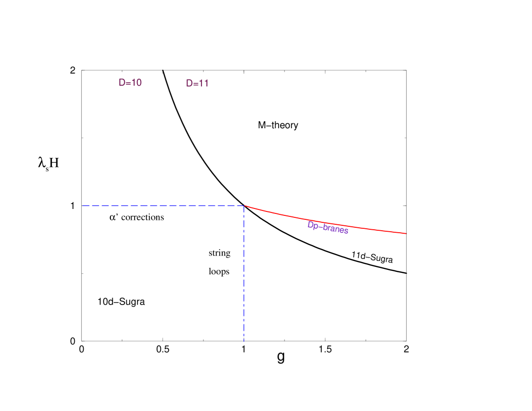
Figure 1: The phase diagram for M-theory compactified on $S^{1}$.

On the 10-dimensional side, the region near the origin corresponds to low curvatures and weak couplings, and here the description in terms of the lowest order closed string effective action is adequate. String theory provides two kind of corrections to this 10D supergravity action: $\alpha^{\prime}$ corrections, i.e. corrections associated with higher powers of the Riemann tensor, which become important as $\lambda_{s}H$ approaches one, and string loop corrections, which become important as $g$ approaches one. The dashed lines in fig. 1 limit the validity of the perturbative expansion of the low-energy 10-dimensional string effective action.

On the 11-dimensional side, we can distinguish two regions separated by the curve $\ell_{p}H=1$, where $\ell_{p}\sim g^{1/3}\lambda_{s}$ is the 11-dimensional Planck length. The curve is indicated by the label “D$p$-branes”. If we cross the border between the 10D and the 11D regions at large values of $g$ and we are just above the line identified by the relation $\lambda_{s}H=g^{-1}$, an adequate description is still provided by 11-dimensional supergravity. In fact, now the large $g$ limit is under control since it corresponds to the decompactification limit $R_{11}\gg\lambda_{s}$, and at the same time $H\ll M_{p}$, where $M_{p}=1/\ell_{p}$ is the 11-dimensional Planck mass. The 10D gravitons (to be identified with the 11-D gravitons with vanishing momentum along the 11^th dimension) are still the relevant massless modes. Quantum production of D0-branes by the gravitational field takes place and a new degree of freedom appears, which is the graviton with $p_{11}$ non vanishing, or equivalently a gas of weakly interacting D0-branes. As we will compute in sect. 3, this mode becomes tachyonic at the transition, signalling the opening up of the new dimension.

This description will eventually break down if the system approaches the curve labelled “D$p$-branes”. If we approach this curve at fixed $H$ and increasing $g$ more and more KK-modes must be included as light degrees of freedom and more and more D$p$-brane states become light because their tensions decrease as $g^{-1}$. However – as we will show in section 5 – something dramatic happens even if we approach the curve from below at fixed $g$ and increasing $H$: all the D$p$-branes become tensionless and they become the fundamental degrees of freedom! Therefore the Universe enters a regime of D$p$-brane domination that leads the system to a transition into the full M-theory regime.

Thus, moving from the 10D Sugra region into the 11D Sugra region and then toward the full M-theory regime, the basic modes are at first the massless closed string modes, then both massless closed string modes and D0-branes (i.e. 11-dimensional gravitons), and finally only D$p$-branes.

Of course, what is the proper description in the full M-theory region is still an open question (with matrix theory [11] being a very interesting candidate), but in the following we will argue that its knowledge is not really necessary since our findings seem to indicate that the line labelled “D$p$-branes’ in fig. 1 was never crossed during the evolution of the Universe.

3 D0-branes production and the opening of the $11^{th}$ dimension

We now discuss the crossover between the 10D-Sugra and 11D-Sugra regime. Let us begin by recalling a few well known facts about the correspondence between 11-dimensional fields or branes compactified on $S^{1}$, and 10-dimensional type IIA quantities [2]. On the 10-dimensional side, the fields are the 10D metric $g_{\mu\nu}$, the dilaton $\phi$, the antisimmetric tensor field $B_{\mu\nu}$ and RR tensor fields, plus the fermionic partners. On the 11-dimensional side, the fields are the metric $g_{MN}$, with $M=(\mu,11)$, a 3-form field $A_{MNR}$ and the gravitino, and there are a 2-brane and a 5-brane.

The correspondence between the fields is given by dimensional reduction from 11D supergravity [13], and in particular the dilaton of the 10D theory is related to the $g_{11,11}$ component of the metric. To obtain directly the relation between the 10D metric and dilaton and the 11D metric we can neglect for the moment $g_{\mu,11}$, which produces a RR one-form, keeping only the components $g_{\mu\nu}$ of the 11D metric $g_{MN}$, $M=(\mu,11),\mu=0,\ldots 9$, and the component $g_{11,11}\equiv b^{2}$, so that $b$ is the scale factor of the $11^{th}$ dimension. Then a simple computation shows that the 11-dimensional Einstein-Hilbert action becomes

$$S=\frac{1}{2\lambda_{s}^{8}}\int d^{10}x\sqrt{-g^{(10)}}\,\,bR^{(10)}\,.$$ (4)

The scale factor $b$ of the $11^{th}$ dimension looks non-dynamical at a first sight, since it appears without derivatives. One should remember though that the 10-dimensional Ricci scalar $R^{(10)}$ contains second derivatives of the metric. The fact that $b$ is indeed dynamical is made evident by a conformal rescaling $g^{(10)}_{\mu\nu}\rightarrow b^{-1}g^{(10)}_{\mu\nu}$. Defining the dilaton $\phi$ from

$$e^{\phi}=b^{(D-3)/2},$$ (5)

where in our case $D=9$, one finds

$$S=\frac{1}{2\lambda_{s}^{8}}\int d^{10}x\sqrt{-g^{(10)}}\,e^{-\phi}\left[R^{(10)}+(\partial\phi)^{2}\right]\,,$$ (6)

which is the effective action of string theory in the gravity–dilaton sector.

The KK field $g_{\mu,11}$ becomes instead a RR one-form $C_{\mu}$ in type IIA. The object which is charged under $C_{\mu}$ in type IIA is the D0-brane, which therefore from the 11-dimensional point of view is coupled to $g_{\mu,11}$ and therefore is a supergraviton with momentum $p_{11}=1/R_{11}$. The state with momentum $p_{11}=n/R_{11}$, in the type IIA language becomes a collection of $n$ D0-branes, an interpretation made possible by the fact that $n$ D0-branes have a marginally bound state with a mass $n$ times the single D0-brane mass $1/(g\sqrt{\alpha^{\prime}})$, and this result receives no perturbative or non-perturbative correction because this state is BPS saturated.

The transition at the 10D Sugra/11D Sugra border is therefore different from the example discussed in the introduction, since it does not involve a dramatic reshuffling of degrees of freedom. The 10D gravitons are still relevant massless modes, but they are now embedded in 11D-gravitons with vanishing momentum in the $11^{th}$ dimension. At first sight, one might think that we can neglect the states with non-vanishing momentum in the $11^{th}$ dimension (i.e. D0-branes), and that we can limit ourselves to 11D gravitons, and look for 11D-cosmological solutions, spatially constant in all directions including the 11^th (for work on 11D solutions see refs. [14]).

However, the situation is more complicated and the fields of 11-dimensional supergravity are not the only relevant modes: in a gravitational field, D0-branes can become massless and, beyond a critical field, tachyonic.

The fact that D0-branes are non-negligible degrees of freedom in the 11D Sugra regime is already suggested by the computation in Ref. [12] of D0-branes pair production. This can be computed first of all in the 11D-Sugra region, considering for instance a process of graviton-graviton scattering with production of D0-branes. While from the 10D point of view this process is inelastic and non-perturbative, from the 11-dimensional point of view it is simply an elastic scattering process in which the final 11D gravitons have a component of the momentum along the $11^{th}$ dimension. The process can therefore be computed reliably, and clearly the production of pairs of D0-branes is not suppressed. In Ref. [12] the production rate of D0-branes has also been computed using matrix string theory. The result, which gives an unsuppressed rate, is found to be in agreement with the supergravity calculation, but is expected to be valid more in general in the M-theory regime.

In the early Universe, to produce D0-branes is not even necessary to consider a scattering process. A time-varying gravitational field produces particles. The general mechanism is the existence of a non-trivial Bogoliubov transformation between the in and out vacuum. The amplification of vacuum fluctuations which takes place in any cosmological background will produce a spectrum of 11-dimensional supergravitons. From the 10D point of view, this means that a background of both 10D gravitons and D0-branes are created from the vacuum.

The analysis is similar to the one performed at finite temperature to identify the states which become tachyonic at the Hagedorn temperature in the weak coupling regime [15, 16, 17]. Identifying the D0-branes with gravitons with a non-vanishing momentum along the 11^th dimension, we need to know the closed string spectrum in a gravitational field at oscillator level 1, corrisponding to gravitons, and with non-vanishing KK momentum. However, solving the equations of motion and constraints of strings in generic curved spacetime is a prohibitive task. One can try the expansion [18, 19] $X^{\mu}(\sigma,\tau)=x^{\mu}(\tau)+Y^{\mu}(\sigma,\tau)$, where $x^{\mu}$ defines the motion of a point-particle and $Y^{\mu}$ describes the finite-string size effects. The physical idea behind this expansion is that a small-enough string should follow closely the point-particle geodetic.

At second order in $Y^{\mu}$ and large values of the scale factor of the Universe $a$ (or at large times), the components $Y^{i}$ ($i=1,\cdots,D$) satisfy a particularly simple equation. Defining $\chi^{i}=aY^{i}=\sum_{n}\chi_{n}^{i}e^{in\sigma}$, one gets [19]

$$\ddot{\chi}_{n}^{i}=\left[-n^{2}+\ell^{2}\frac{\ddot{a}}{a}\right]\chi_{n}^{i},$$ (7)

where the dot is the derivative with respect to world-sheet time, while $\ell$ is a parameter of the background configuration around which we are expanding. We can physically interprete it as the total length of the string and, at least for string not highly excited, we can take $\ell\sim\lambda_{s}$.

Specializing – for simplicity – to the case of isotropic de Sitter geometry with constant $H$, the frequency modes of the string are given by [18, 19]

$$\omega_{n}=\left(n^{2}-\ell^{2}H^{2}\right)^{1/2}.$$ (8)

The mass shell condition of the closed string modes can be written, at large times (when the world-sheet time becomes proportional to conformal time [19]) as

$$\frac{1}{4}M^{2}=\frac{m^{2}}{4R_{11}^{2}}+\frac{R_{11}^{2}}{(2\alpha^{\prime})^{2}}q^{2}+\frac{1}{2\alpha^{\prime}}\left(N+\widetilde{N}-2c\right),$$ (9)

where $\sqrt{2\alpha^{\prime}}=\lambda_{s}$; $m$ and $q$ are integers which give the momentum and winding in the 11^th dimension, $N=\sum_{n=1}^{\infty}\omega_{n}a_{n}^{\dagger}\cdot a_{n}$ with $a_{n}^{\mu},a_{n}^{\mu\dagger}$ conventionally normalized harmonic oscillator operators for the left handed modes, and similarly $\widetilde{N}$ for the right-handed modes, and $N-\widetilde{N}=mq$; $c$ is the normal ordering constant.

A collection of $N$ D0-branes is a 11D-graviton with $N$ units of momentum in the $11^{th}$ dimension and therefore has oscillator level $n=1$, KK quantum number $m=N$, and winding number $q=0$, (and therefore $N=\widetilde{N}$). Its mass is

$$M^{2}=\frac{N^{2}}{R_{11}^{2}}+\frac{8}{\lambda_{s}^{2}}\left[\left(1-\ell^{2}H^{2}\right)^{1/2}-c\right]\,.$$ (10)

The constant $c$ comes from normal ordering and we will set $c=1$ as in flat space.

Eq. (10) shows various kind of instabilities. First of all, for large enough Hubble constant $H$, the frequencies $\omega_{n}$ become imaginary and then the low frequency modes become unstable. This instability has been discussed in [19] and has partly motivated the pre-big-bang scenario [5]. Furthermore, setting $N=0$, we see that, even for small values of $\ell H$, the graviton becomes tachyonic, with $M^{2}\simeq-4(\ell^{2}/\lambda_{s}^{2})H^{2}\lower 3.01385pt\hbox{$\;\stackrel{{\scriptstyle\textstyle<}}{{\sim}}\;$}-4H^{2}$. Physically, this is consistent with the fact that in de Sitter space gravitons are produced by amplification of vacuum fluctuations, with an effective temperature $H/(2\pi)$.

Here we are interested in the appearance of further tachyonic states, with non-zero momentum in the 11^th dimension. Expanding for $\ell H\ll 1$, for $N=1$ a new tachyonic mode appears at

$$H\simeq\frac{1}{2}\frac{\lambda_{s}}{\ell}\frac{1}{R_{11}}\lower 3.01385pt\hbox{$\;\stackrel{{\scriptstyle\textstyle<}}{{\sim}}\;$}\frac{1}{2}\frac{1}{R_{11}}\equiv H_{c}$$ (11)

which corresponds to the solid line of fig. 1. Note that $\ell H_{c}\sim\lambda_{s}/(2R_{11})=1/(2g)$ so that our expansion for $\ell H\ll 1$ is consistent in the region $g\gg 1$. Without relying on this expansion, we read from eq. (10) that a tachyon indeed exists, for each $N$, if $N^{2}/R_{11}^{2}-8/\lambda_{s}^{2}<0$, or if $g>N/(2\sqrt{2})$. The first new tachyon, $N=1$, appears if $g>1/(2\sqrt{2})$, which is consistent with the fact that we are working at $g>1$ (actually, we could now take $g=1/(2\sqrt{2})$ as the more precise location of the ‘triple point’ in the phase diagram, fig. 1).

This instability is also manifest in the closed string vacuum-vacuum transition amplitude at one-loop, ${\cal A}_{\rm 1-loop}$. The amplitude is given by

$${\cal A}_{\rm 1-loop}=iV_{d}\int\frac{d\tau d\bar{\tau}}{4\tau_{2}}(4\pi^{2}\alpha^{\prime}\tau_{2})^{-d/2}\sum z^{N-1}\bar{z}^{\widetilde{N}-1}\,,$$ (12)

where $\tau=\tau_{1}+i\tau_{2}$, the integration is over the fundamental region of the torus, $z=\exp(2\pi i\tau)$ and the sum is over the physical closed string spectrum. The limit $\tau_{2}\rightarrow\infty$ is dominated by the lightest modes [22]

$${\cal A}_{\rm 1-loop}=2\pi iV_{d}\int^{\infty}\frac{d\tau_{2}}{2\tau_{2}}(4\pi^{2}\alpha^{\prime}\tau_{2})^{-d/2}\sum_{i}\exp(-\pi\alpha^{\prime}m_{i}^{2}\tau_{2})\,.$$ (13)

and diverges if a tachyon, $m_{i}^{2}<0$, is present. The instability signals that new channels are opening up. Therefore, when the horizon of the Universe contracts approaching the critical value $H_{c}^{-1}$, the effective theory from 10-dimensional becomes 11-dimensional and this is signalled by the copious and unsuppressed gravitational production of D0-branes carrying longitudinal momentum $p_{11}=1/R_{11}$ and – eventually – states carrying KK momentum $p_{11}=N/R_{11}$ which are properly described as marginally bound states of $N$ D0-branes. At $H\sim H_{c}$ and strong coupling the Universe enters a phase where the energy density is dominated by the gas of branes produced at large curvature. The production of this gas has clearly a regularizing effect on the growth of the curvature in a pre-big-bang type scenario. From the 10D point of view, the energy density grows until it reaches a critical value, where it is dissipated by generating D0-branes. Probably, inhomogeneities in the field configuration play here an important role, as seeds for D0-branes formation.

From the 11D point of view, instead, above a critical value the classical field, which was constrained to live in 10D, starts to spread over the 11^th dimension, and its energy density consequently drops. When the Universe enters this phase of D0-brane domination the regime of growing curvature is significantly slowed down (see also [23]).

The transition at high curvature and non-perturbative regime into a new phase of gas of D0-branes that we have just described is reminiscent of the Hagedorn transition that takes place at finite temperature in the matrix model [11] of $N$ D0-branes. At low temperatures, there is a string phase where the D0-branes are spread out to form a membrane wound around a compact direction. In this phase the ground state must be that of a IIA string with a specified value of the string tension. The light modes are those of a string. At high temperatures the energy in the strings is overwhelmingly found in the highest mode that can be excited with that energy. However, in the matrix model there is a cut-off on the mode number. Thus in the partition function there is a natural cut-off in the energy integral above which the discrete nature of the string becomes important and at this point one has to go back to the original matrix model. What happens is that, at high temperatures, the D0-branes prefer to cluster at one point, thus the string ceases to exist. One can think of this as the tendency of the string to shrink to zero size and disintegrate into a bunch of D0-branes. The light degrees of freedom are therefore the massless modes which are just the fluctuations about the origin of the $N^{2}$ matrix elements. This phase transition can be identified with the Hagedorn transition for the IIA string constructed out of the $N$ D0-branes [24].

4 The D$p$-brane phase

The goal of this section is to describe the dynamics of the system when the curvature of the Universe approaches values of the order of $\ell_{p}^{-2}$. To do so, we have first to study the dynamics of D$p$-branes in curved spacetime.

4.1 D$p$-brane dynamics in curved background

The action governing the dynamics of a Dirichlet $p$-brane is [2, 25]

$$S=-T_{p}\int d^{p+1}\xi\,e^{-\phi}\sqrt{-\det(G_{\alpha\beta}+B_{\alpha\beta}+2\pi\alpha^{\prime}F_{\alpha\beta})}\,,$$ (14)

where $T_{p}^{-1}=\sqrt{\alpha^{\prime}}(2\pi\sqrt{\alpha^{\prime}})^{p}$, $\xi^{\alpha}$ ($\alpha=0,\ldots,p$) parametrize the D-brane world-volume, $G_{\alpha\beta}$ is the induced metric

$$G_{\alpha\beta}=g_{\mu\nu}(X)\partial_{\alpha}X^{\mu}\partial_{\beta}X^{\nu},$$ (15)

while $B_{\alpha\beta},F_{\alpha\beta}$ are the pull-back of $B_{\mu\nu},F_{\mu\nu}$ to the brane. If we consider a flat background metric, $g_{\mu\nu}=\eta_{\mu\nu}$, and we assume that the extrinsic curvature of the brane is small, then we can separate the $D+1$ coordinates $X^{\mu}$ into $p+1$ longitudinal components $X^{\mu}(\xi)=\xi^{\mu}$ ($\mu=0,\ldots,p$) and $(D-p)$ transverse coordinates $X^{a}$ (where $D$ is the appropriate number of spatial dimensions). The induced metric then becomes

$$G_{\alpha\beta}\simeq\eta_{\alpha\beta}+\partial_{\alpha}X^{a}\partial_{\beta}X^{a}\,.$$ (16)

Neglecting $B_{\mu\nu}$ and expanding to second order in $\partial X$ and $F$ one gets [2]

$$S=-\tau_{p}V_{p}-\int d^{p+1}\xi\,\left[\frac{\tau_{p}}{2}\partial_{\alpha}X^{a}\partial^{\alpha}X^{a}+\frac{1}{4g_{YM}^{2}}F_{\alpha\beta}F^{\alpha\beta}\right]\,,$$ (17)

where $\tau_{p}=T_{p}/g$ is the brane tension, $V_{p}=\int d^{p+1}\xi$ is the brane volume, $g_{YM}^{2}=(g/\sqrt{\alpha^{\prime}})(2\pi\sqrt{\alpha^{\prime}})^{p-2}$ and $g=e^{\phi}$. The term $\tau_{p}V_{p}$ is the mass of the D-brane, while the fields $A_{\alpha}$ and $X^{a}$ describe the D-brane fluctuations. The longitudinal components $A_{\alpha}$ of $A_{\mu}$ are governed by a $U(1)$ gauge theory living on the brane, while the transverse displacements $X^{a}$ are $(D-p)$ world-volume scalars.

We now repeat the procedure for a curved background metric $g_{\mu\nu}$. We concentrate on the transverse coordinates $X^{a}$ and we set $F_{\mu\nu}=B_{\mu\nu}=0$. The most convenient generalization of the notion of transverse coordinates to the case of a curved background is provided by Riemann normal coordinates. Given a brane configuration $\bar{X}^{\mu}(\xi)$, arbitrary fluctuations transverse to this configuration are parametrized by $(D-p)$ world-volume scalars $\phi^{a}(\xi)$ as

$$X^{\mu}(\xi)=\bar{X}^{\mu}(\xi)+\bar{n}^{\mu}_{a}(\xi)\phi^{a}(\xi),$$ (18)

where $\bar{n}_{a}^{\mu}(\xi)$ ($a=1,\ldots,(D-p)$) are the $(D-p)$ vectors normal to the brane at the point $\bar{X}(\xi)$. The expansion of the metric in Riemann coordinates is [26]

$$g_{\mu\nu}(X)=\bar{g}_{\mu\nu}-\frac{1}{3}\phi^{a}\phi^{b}\bar{R}_{\mu\rho\nu\sigma}\bar{n}_{a}^{\rho}\bar{n}_{b}^{\sigma}+{\cal O}(\phi^{3})\,,$$ (19)

where the overbar indicates that the quantity is evaluated at $\bar{X}$. If the extrinsic curvature of the membrane is small, the normal vectors are $\bar{n}_{a}^{\rho}\simeq\delta_{a}^{\rho}$, and therefore

$$g_{\mu\nu}(X)=\bar{g}_{\mu\nu}-\frac{1}{3}X^{a}X^{b}\bar{R}_{\mu a\nu b}+{\cal O}(X^{3}).$$ (20)

(We now use the notation $X^{a}\equiv\phi^{a}$, so that from now on $X^{a}$ are the fluctuations over $\bar{X}$, rather than $X^{\mu}$ for $\mu=a$. We also use the sign conventions $\eta_{\mu\nu}=(-,+,\ldots,+),R^{\mu}_{\hskip 5.69054pt\nu\rho\sigma}=\partial_{\rho}\Gamma^{\mu}_{\nu\sigma}+\ldots$). Again, we specialize to the de Sitter background for simplicity, but our conclusions can be generalized to any specific situation where $H^{2}$ is the typical curvature scale. The metric is

$$ds^{2}=a^{2}(\eta)(-d\eta^{2}+dx_{i}dx^{i}).$$ (21)

The scale factor is $a(\eta)=-1/(H\eta)$, and $\eta$ is conformal time, $\eta<0$. The Riemann tensor is given by $\bar{R}_{\mu\nu\rho\sigma}=H^{2}(\bar{g}_{\mu\rho}\bar{g}_{\nu\sigma}-\bar{g}_{\mu\sigma}\bar{g}_{\nu\rho})$ and the induced metric in the limit of small extrinsic curvature is then

$$G_{\alpha\beta}=F_{\alpha\beta}+f_{ab}\partial_{\alpha}X^{a}\partial_{\beta}X^{b},$$ (22)

where

$$F_{\alpha\beta} = a^{2}\left(1-\frac{1}{3}H^{2}a^{2}X^{2}+{\cal O}(X^{4})\right)\eta_{\alpha\beta},$$ (23)

$$f_{ab} = a^{2}\left[\left(1-\frac{1}{3}H^{2}a^{2}X^{2}\right)\delta_{ab}+\frac{1}{3}H^{2}a^{2}X_{a}X_{b}+{\cal O}(X^{4})\right]\,,$$ (24)

and $X^{2}=\sum_{a}X^{a}X^{a}$. Here $X^{a}$ represents the comoving coordinate and $X_{p}^{a}=a(\eta)X^{a}$ is the physical coordinate, which expands with the scale factor.

We are now in the position to compute $\det G_{\alpha\beta}$. Retaining only terms up to second order in $X$ and $\partial X$ we get

$$S=-\tau_{p}V_{p}-\tau_{p}\int d^{p+1}\,\xi a^{p+1}\,\left[\frac{1}{2}\eta^{\alpha\beta}\partial_{\alpha}X^{a}\partial_{\beta}X^{a}-\frac{(p+1)a^{2}H^{2}}{6}X^{a}X^{a}\right]\,.$$ (25)

In flat space the fields $X^{a}$ are massless, see eq. (17), since they are the Goldstone bosons of broken translation invariance in the transverse directions. Recalling that our signature is $\eta_{\alpha\beta}=(-,+,\ldots,+)$, we see that in curved space the pseudo-Goldstone bosons of broken translation invariance, $X_{p}=aX$, get a tachyonic mass

$$m^{2}=-\frac{(p+1)H^{2}}{3}\,.$$ (26)

The situation is very similar to the thermal tachyon which occurs at the Hagedorn temperature [15, 16]. In that case a condensate of winding states forms when the periodic imaginary times becomes too small. In the present case the tachyon forms because of the nontrivial geometry of the spacetime.

Switching to cosmic time $t$ and expanding $X^{a}(t,\vec{\xi})=\sum_{k}X^{a}_{k}(t)\exp(i\vec{k}\cdot\vec{\xi})$, the equation of motion for the comoving modes $X^{a}_{k}$ is

$$\ddot{X}^{a}_{k}+(p+2)H\dot{X}^{a}_{k}+\left(\frac{k^{2}}{a^{2}}-\frac{p+1}{3}H^{2}\right)X^{a}_{k}=0\,,$$ (27)

where the dot stands for the derivative with respect to cosmic time $t$. Let us first discuss the behaviour of the mode $X^{a}_{k}$ in the absence of the tachyonic mass, that is dropping by hand the term $\sim(p+1)H^{2}/3$ in eq. (27). The behaviour of a mode $X^{a}_{k}$ is very simple. As long as the physical wavelength $ak^{-1}$ of a mode is inside the Hubble radius, $aX^{a}_{k}$ is an oscillating function whose amplitude descreases as $e^{-\frac{p}{2}Ht}$. As the physical wavelength grows it crosses the Hubble radius and the comoving amplitude $X^{a}_{k}$ becomes frozen, so the physical amplitude grows as $a$. Returning to the case of interest in which the tachyonic mass is present, as long as the physical wavelength is well inside the horizon, again the physical amplitude $aX^{a}_{k}$ decreases as $e^{-\frac{p}{2}Ht}$. However, as the physical wavelength crosses the horizon, the comoving amplitude does not remain frozen, but instead grows exponentially, so the transverse physical amplitude grows faster than the scale factor $a$ and therefore faster than the physical coordinates defining the brane. Therefore, any comoving transverse fluctuations of the D$p$-brane – even though initially damped – will eventually grow and give rise to an instability. As the brane is stretched by the expansion of the Universe, transverse fluctuations grow so quickly that the D$p$-brane cannot be considered as a static object (in comoving coordinates) any longer. In fact the brane looses its own identity as physical transverse fluctuations grow faster than the physical coordinates defining the D$p$-brane.

To get further insight and to follow the system beyond the approximation of small transverse fluctuations, we must compute higher order terms in the tachyon effective potential. Let us consider the case of $X^{a}$ not necessarily small but $\partial_{\alpha}X^{a}=0$, so that we are interested in the mass of the brane itself, which in flat space is the term $\tau_{p}V_{p}$ in eq. (17), rather than in the kinetic term of the fields $X^{a}$. For symmetric spaces like de Sitter space, the expansion of the metric in Riemann coordinates can be written explicitly at all orders in $X^{a}$ [26]

$$g_{\mu\nu}=\bar{g}_{\mu\nu}-\frac{1}{2}\sum_{k=1}^{\infty}\frac{(-1)^{k}2^{2k+2}}{(2k+2)!}m_{\mu}^{\sigma_{1}}m_{\sigma_{1}}^{\sigma_{2}}\ldots m_{\sigma_{k-1}\nu}\,,$$ (28)

where

$$m_{\mu\sigma}=\bar{R}_{\mu ab\sigma}X^{a}X^{b}=(\eta_{\mu b}\eta_{\sigma a}-\eta_{\mu\sigma}\eta_{ab})y^{a}y^{b}\,.$$ (29)

The last equality holds for de Sitter space and we have defined $y^{a}=HX_{p}^{a}$. If we set $\partial_{\alpha}X^{a}=0$, the induced metric $G_{\alpha\beta}$, for small extrinsic curvature is simply equal to $g_{\mu\nu}$ with $\mu=\alpha,\nu=\beta$ (recall that $\mu=(\alpha,a)$ where $\alpha$ runs over the value zero and the longitudinal directions, while $a$ runs over the transverse directions). Eq. (28) then simplifies considerably since, if the index $\mu$ has a ‘longitudinal’ value $\alpha$, then $m_{\mu}^{\sigma_{1}}$ is non-vanishing only if also $\sigma_{1}$ has a longitudinal value $\gamma$, and $m_{\alpha}^{\gamma}=-\delta_{\alpha}^{\gamma}y^{2}$, with $y^{2}=y^{a}y^{a}$, and so all indices $\sigma_{1},\ldots\sigma_{k-1}$ in eq. (28) are longitudinal. As a result, we find $G_{\alpha\beta}=f(y)\eta_{\alpha\beta}$ with

$$f(y)=1-2\sum_{k=1}^{\infty}\frac{(2y)^{2k}}{(2k+2)!}=2-\frac{\sinh^{2}y}{y^{2}}\,.$$ (30)

The action in the limit of small $\partial_{\alpha}X^{a}$ is therefore

$$S=-\int d^{p+1}(a\xi)\,\tau_{p}f^{\frac{p+1}{2}}(HX_{p})\,.$$ (31)

The function $f(y)$ decreases monotonically, has the perturbative expansion $f(y)=1-(1/3)y^{2}+\ldots$ around $y=0$ and vanishes at $y=y_{0}\simeq 1.49$. Therefore, in de Sitter spacetime the “potential” $f(y)$ of the tachyon field $y$ is negative around the origin $y=0$ and the field rolls down away from it.

The existence of the critical point $y_{0}$ might have very interesting implications. If $HX_{p}$ approaches the critical value, the D$p$-branes become almost tensionless, for any value of $p$. This renormalization of the brane tension is similar to what happens to $(n,1)$ strings, bound states of one D-string and $n$ fundamental strings. This system may be described by a D-string with a world volume electric field $E$ turned on. As the electric field approaches its critical value, $n$ becomes large. The effective tension of the $(n,1)$ string is renormalized by the electric field, $T_{eff}=T_{1}(1-E^{2})$  [27].

Our result does not come as a surprise since the analysis performed above for small fluctuations already suggested that the D$p$-brane violently fluctuate along the transverse directions paying no price in energy. Once some D$p$-branes are formed – as we expect at strong coupling – they fluctuate along their transverse directions. Long-wavelength transverse fluctuations grow and this growth is probably accompanied by a huge production of light pseudo-Goldstone bosons of the broken translation invariance. Since the branes become tensionless, it becomes easier and easier for the gravitational background to produce further massless D$p$–branes. On the other hand, when the transverse sizes of the D$p$-branes become larger than the horizon, the branes presumably break down and decay. Smaller branes are continuously created and the situation is quite similar to what happens in a network of (cosmic) strings. One can also envisage various other dynamical phenomena like the melting of two or more branes when they are closer than the horizon distance.

Furthermore, we know that D0-branes carry an halo around them of size $\sim\ell_{p}$ even though they appear point-like. Therefore, in the context of M-theory it is not sensible to require that the fluctuations are smaller then a value of order of the 11-dimensional Planck length $\ell_{p}$. Even in the presence of ‘minimal’ fluctuations with $\langle X^{2}\rangle\sim\ell_{p}^{2}$, at $H\sim 1/\ell_{p}$ there must be a change of regime. In fact – if $H$ approaches the line labelled “D-branes” in fig. 1 – $HX_{p}$ approaches its critical value. The stage of increasing curvature should therefore come to an end and be replaced by a phase where the Universe is dominated by a gas of D$p$-branes and their excitations. Let us observe that – even if we have discussed D-branes with a neglegible extrinsic curvature – the argument can be generalized to arbitrarily bent D-brane. For membranes, this has been done in [28], where it has been shown that the extrinsic curvature tensor $K_{\alpha\beta}$ gives a further tachyonic contribution to the mass squared, $m^{2}\sim~{}-K_{\alpha\beta}K^{\alpha\beta}<0$.

It is intriguing that the limiting value of the curvature is consistent with considerations based on the holographic principle as we now discuss.

4.2 The holographic principle and cosmology

Recent developments in black hole physics and in string theory have inspired the so-called holographic principle [29, 30]. It requires that the degrees of freedom of a given spatial region live not in the interior as in ordinary quantum field theory, but on the surface of the region. The cosmological version of the holographic principle [31] requires that the degrees of freedom of a spatial volume of coordinate size the horizon length $\ell_{H}$ should not exceed the area of the horizon in Planck units. If one accepts this argument, there are several implications when applying it to 11-dimensional theories.

The holographic principle leads us to conjecture that, no matter what is responsible for the appearance of branes as fundamental degrees of freedom in the Universe and no matter what is the dynamics of the system after it enters the phase of brane domination, the horizon length $\ell_{H}$ cannot be smaller than the 11-dimensional Planck length $\ell_{p}$. Indeed, let us call the spatial direction $x^{11}$ longitudinal and the nine remaining dimensional coordinates transverse. Suppose that the transverse area is occupied by a system of longitudinal momentum $p_{11}$. Being the number of degrees of freedom certainly larger than the number $(p_{11}R_{11})$ of KK modes excited in the 11^th dimension, the holography principle imposes the following bound

$$\left(\frac{\ell_{H}}{\ell_{p}}\right)^{9}>p_{11}R_{11}>1,$$ (32)

or

$$\ell_{H}>\ell_{p}.$$ (33)

The last inequality of eq. (32) has been obtained using the fact that D0-branes carry a longitudinal momentum equal to $1/R_{11}$.

To motivate even further our conjecture (33), we can give it the following simple interpretation. As we have seen above, in the regime of growing large curvature the horizon length $\ell_{H}$ is contracting and the Universe becomes populated by a gas of branes. As in this gas two D0-branes move way from each other, they transfer continuosly their energy to any open strings that happen to stretch between them. A virtual pair of open strings can thus materialize from the vacuum and slow down, or even stop completely the motions of the branes (see Bachas in [2]). This phenomenon is similar to the more familiar pair production in a background electric field [33] and to the appearance of an instability in the D-brane self-energy at finite temperature and weak coupling regime at the Hagedorn temperature [34].

We believe that the onset of the dissipation puts a lower limit on the distance scales probed by the scattering of D0-branes and it turns out that the dynamical size of D0-branes is comparable to the inverse cubic root of the membrane tension, i.e. to the $11^{th}$-dimensional Planck scale of M-theory! It is therefore clear that the horizon length cannot contract to values smaller than $\ell_{p}$, since at this scale the dissipation sets in, slowing down the growth of the curvature and – ultimately – stopping it.

5 Discussion and conclusions

We now discuss the relevance of our analysis for different cosmological issues. Our considerations can be applied for instance to the pre-big-bang scenario [5]. The cosmological evolution starts at $t\rightarrow-\infty$ in the weak coupling, low curvature region, i.e. near the origin in fig. 1, where we can use the low energy effective action of string theory, neglecting $\alpha^{\prime}$ and loop corrections. In the string frame (i.e. when the Einsten term in the action has a factor $e^{-\phi}$ in front) the general homogeneous vacuum solution has the form [5]

$$a_{i}(t)\sim(-t)^{\alpha_{i}}\,,\hskip 28.45274pt\phi(t)\sim\phi_{0}-\gamma\log(-t)\hskip 28.45274pt(-\infty<t<0),$$ (34)

(where $a_{i}(t)$ are the FRW scale factors) which can also be generalized to the non-homogeneos case [35]. The constants $\alpha_{i},\gamma$ satisfy the conditions

$$\sum_{i=1}^{D}\alpha_{i}^{2}=1\,,\hskip 28.45274pt\gamma+\sum_{i=1}^{D}\alpha_{i}=1\,.$$ (35)

Setting $\gamma=0$ one recovers the well known Kasner solution of general relativity. In the isotropic case, the Kasner condition fixes $\alpha=\pm 1/\sqrt{D},\gamma=1\mp\sqrt{D}$. The solution with the lower sign is superinflationary, $\dot{H}>0$, with a growing dilaton, and formally reaches a singularity as $t\rightarrow 0^{-}$. In the $(H,g)$ plane, these solutions read

$$H=\frac{1}{\sqrt{D}}\left(\frac{g}{g_{0}}\right)^{\frac{1}{1+\sqrt{D}}}\,,$$ (36)

where $g_{0}$ is the initial coupling. For $D=9$, it has the form $H\sim g^{1/4}$, as shown in fig. 2, for two different values of the initial conditions.

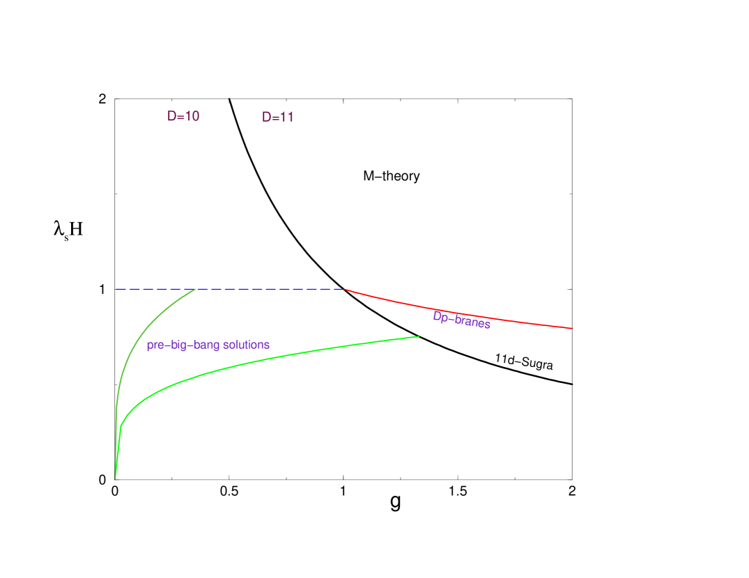
Figure 2: The phase diagram of M-theory and the lowest order pre-big-bang solutions $H\sim g^{1/4}$, for two different values of the initial conditions.

The classical solutions displayed in fig. 2 are only valid close to the origin of the $(H,g)$ plane. As $\lambda_{s}H$ or $g$ approach one, the form of the solutions is determined by $\alpha^{\prime}$ and loop corrections [6, 7]. Various arguments, based both on the study of perturbative $\alpha^{\prime}$ corrections and on the backreaction due to massive string modes [7], indicate that the evolution on the 10D side and weak coupling cannot go beyond the region $\lambda_{s}H\sim 1$, see fig. 2. If the solution reaches this regime, the subsequent evolution typically has $g$ increasing and $H$ constant or decreasing. On the strong coupling side of the 10D region, on the other hand, our results suggest that, even if loop corrections should not stop $H$ and $g$ from growing, a change of regime will take place at the latest along the curve $\lambda_{s}H=1/g$, because of the huge production of relativistic D0-branes. A new radiation-dominated regime is expected to take over when the energy density of the light D0-branes becomes comparable to the critical energy density for closing the Universe. Similar considerations have been put forward in ref. [36] in the context of a 4D compactification of string theory at weak coupling.

Further investigations are needed to understand whether the evolution may cross into the 11D region – and possibly approach the line labelled “D$p$-branes”. If so, we think $H=1/\ell_{p}$ provides the largest value probed during the evolution.

Our results may be also relevant for the cosmology of the so-called brane world scenario. It has recently been realized that the traditional connection in perturbative string theory between the string scale and the Planck mass, $M_{s}=\frac{1}{2}\alpha_{GUT}^{1/2}M_{p}$ does not need to be applied to all string vacua [37, 38, 39, 40, 41, 42, 43, 44, 45, 46]. A possibility that has attracted recently much attention is lowering the string scale down to the weak scale, $M_{s}\sim$ TeV, thus giving chances of testing string theory at accelerators. In these scenarios, branes play a fundamental role. Indeed, in type I string theory the gravitational sector consists of closed strings propagating in the higher-dimensional bulk, while matter fields consist of open strings living on D5- and D9-branes. Even though reconciling this scheme with the tight constraints from cosmology seems particularly challenging, it is clear that a complete analysis of the cosmology of the TeV-superstring scenario cannot be performed neglecting the presence of fundamental objects such as D-branes. For instance, in the brane world scheme, inflation may automatically take place in the pre-big-bang era and be driven by the dilaton field of the closed sector of type I string theory. As we pointed out, D-branes represent a key ingredient for understanding how the singularity is avoided and how the Universe enters a radiation-dominated regime. Fundamental issues such as the determination of the “reheating” temperature of the Universe after the stringy phase, the stabilization of the dilaton field and of the radii of the extra dimensions may be thoroughlly addressed only including D-branes in the whole picture.

Acknowledgements

We would like to thank S. Dimopoulos, G.F. Giudice, A. Gosh, S. Gukov and especially G. Veneziano for useful conversations. MM thanks the Theory Division of CERN, where part of this work was done, for the kind hospitality. AR would like to thank the International School for Advanced Studies, Trieste, and the Department of Physics, University of Pisa, where part of this work was done, for the kind hospitality.

References

- [1] N. Seiberg and E. Witten, Nucl. Phys. B426 (1994) 19; ibid. B431 (1994) 484.
-
[2]
See for example: J. Polchinski, TASI
lectures on D-branes, hep-th/9611050;
C. Bachas, Lectures on D-branes, hep-th/9806199;
W. Taylor, Lectures on D-branes, Gauge Theory and M(atrices), hep-th/9801182. - [3] A. Strominger, Nucl. Phys. B451 (1995) 96.
- [4] H. Ooguri and C. Vafa, Phys. Rev. Lett. 77 (1996) 3296.
- [5] G. Veneziano, Phys. Lett. B265 (1991) 287; M. Gasperini and G. Veneziano, Astropart. Phys. 1 (1993) 317; Mod. Phys. Lett. A8 (1993) 3701; Phys. Rev. D50 (1994) 2519. An up-to-date collection of references on string cosmology can be found at http://www.to.infn.it/teorici/gasperini/.
- [6] R. Brustein and G. Veneziano, Phys. Lett. B329 (1994) 429; N. Kaloper, R. Madden and K. Olive, Nucl. Phys. B452 (1995) 677; I. Antoniadis, J. Rizos and K. Tamvakis, Nucl. Phys. B415 (1994) 497.
- [7] M. Gasperini, M. Maggiore and G. Veneziano, Nucl. Phys. B494 (1997) 315; R. Brustein and R. Madden, Phys. Lett. B410 (1997) 110; Phys. Rev. D57 (1998) 71; S.J.-Rey, Phys. Rev. Lett. 77 (1996) 1929, and hep-th/9607148; M. Maggiore, Nucl. Phys. B525 (1998) 413; S. Foffa, M. Maggiore and R. Sturani, gr-qc/9804077, Phys. Rev. D, to appear.
- [8] J. Polchinski, Phys. Rev. Lett. 75 (1995) 4724.
- [9] M. Douglas, D. Kabat, P. Pouliot and S. Shenker, Nucl. Phys. B485 (1997) 85.
- [10] F. Larsen and F. Wilczek, Phys. Rev. D55 (1997) 4591.
- [11] T. Banks, W. Fischler, S.Shenker and L. Susskind, Phys. Rev. D55 (1997) 5112.
- [12] S. Giddings, F. Hacquebord and H. Verlinde, hep-th/9804121.
- [13] E. Bergshoeff, M. De Roo, B. De Wit and P. Van Nieuwenhuizen, Nucl. Phys. B195 (1982) 97.
- [14] A. Lukas, B. Ovrut and D. Waldram, Phys. Lett. B393 (1997) 65; Nucl. Phys. B495 (1997) 365; H. Lü, S. Mukherji, C.N. Pope and K.-W. Xu, Phys. Rev. D55 (1997) 7926; N. Kaloper, Phys. Rev. D55 (1997) 3394; N. Kaloper, I. Kogan and K. Olive, Phys. Rev. D57 (1998) 7340.
- [15] B. Sathiapalan, Phys. Rev. D35 (1987) 3277.
- [16] Ya.I.Kogan, JETP Lett. 45 (1987) 709; A.A.Abrikosov,Jr. and Ya.I.Kogan, Sov. Phys. JETP 69 (1989) 235 and Int.J.Mod.Phys. A6 (1991) 1501.
- [17] J. Atick and E. Witten, Nucl. Phys. B310 (1988) 291.
- [18] H.J. de Vega and N. Sanchez, Phys. Lett. B197 (1987) 320.
- [19] N. Sanchez and G. Veneziano, Nucl. Phys. B333 (1990) 253.
- [20] M. Green, J. Schwarz and E. Witten, Superstring theory, Cambridge Univ. Press, cap. 11.
- [21] The sums can be performed explicitly using the results of appendix B of S. Caracciolo and A. Pelissetto, Phys. Rev. D58 105007.
- [22] see e.g. J. Polchinski, String theory, Cambridge Univ. Press, 1998, sect. 7.3.
- [23] S.K. Rama, Phys. Lett. B408 (1997) 91.
- [24] B. Sathiapalan, Mod.Phys.Lett. A13 (1998) 2085.
- [25] R. Leigh, Mod. Phys. Lett. A4 (1989) 2767.
- [26] see for instance A.Z. Petrov, Einstein spaces (Pergamon, Oxford, 1969).
- [27] S. Gukov, I. Klebanov and A. Polyakov, Phys. Lett. B423 (1998) 64.
- [28] B. Carter, J. Geom. Phys. 8 (1992) 53; A. Buonanno, M. Gattobigio, M. Maggiore, L. Pilo and C. Ungarelli, Nucl. Phys. B451 (1995) 677.
- [29] G. ‘t Hooft, Dimensional reduction in Quantum Gravity, in “Salamfest”, pp 284-296 (World Scientific Co, Singapore, 1993).
- [30] L. Susskind, hep-th/9409089.
- [31] W. Fischler and L. Susskind, hep-th/9806039.
- [32] D. Bak and S.J. Rey, hep-th/9811008; A.K. Biswas, J. Maharana and R.K. Pradhan, hep-th/9811051.
- [33] C. Bachas and M. Porrati, Phys. Lett. B296 (1992) 77.
- [34] M. Vàzquez-Mozo, Phys.Lett. B388 (1996) 494.
- [35] G. Veneziano, Phys. Lett. B406 (1997) 297; A. Buonanno, K.A. Meissner, C. Ungarelli and G. Veneziano, Phys. Rev. D57 (1998) 2543; A. Buonanno, T. Damour and G. Veneziano, hep-th/9806230.
- [36] A. Buonanno, K.A. Meissner, C. Ungarelli and G. Veneziano, JHEP 01 (1998) 004.
- [37] E. Witten, Nucl. Phys. B471 (1996) 135.
- [38] J.D. Lykken, hep-th/9603133 .
- [39] N. Arkani-Hamed, S. Dimopoulos and G. Dvali, hep-ph/9803315; I. Antoniadis, N. Arkani-Hamed, S. Dimopoulos and G. Dvali, hep-ph/9804398; N. Arkani-Hamed, S. Dimopoulos and J. March-Russell, hep-th/9809124.
- [40] K. Dienes, E. Dudas and T. Gherghetta, hep-ph/9803466; hep-ph/9806292; hep-ph/9807522.
- [41] K. Dienes, E. Dudas, T. Gherghetta and A. Riotto, hep-ph/9809406.
- [42] G. Shiu and S.H. Tye, hep-th/9805157.
- [43] C. Bachas, hep-ph/9807415.
- [44] Z. Kakushadze and S.H. Tye, hep-th/9809147.
- [45] K. Benakli, hep-ph/9809582 .
- [46] K. Benakli and S. Davidson, hep-ph/9810280 ; D.H. Lyth, hep-ph/9810320.