KUNS-1543 HE(TH) 98/17 hep-th/9811087
M-theory description of 1/4 BPS states
in ${\cal N}=4$ supersymmetric Yang-Mills theory

We discuss BPS states preserving 1/4 supersymmetries of ${\cal N}=4$ supersymmetric Yang-Mills theory as M2-branes holomorphically embedded and ending on M5-branes. We use techniques in electrodynamics to find the M2-brane configurations, and give some explicit examples. In case the M2-brane worldsheet has handles, the worldsheet moduli of the M2-brane is constrained in a discrete manner. Several aspects of multi-pronged strings in type IIB string theory are beautifully reproduced in the M-theory description. We also discuss the relation between the above construction and the D2-brane dynamics in type IIA string theory.

1 Introduction

The recent developments of non-perturbative string theory have provided new powerful tools for analysis of non-perturbative properties of supersymmetric gauge theories. A supersymmetric gauge theory can be studied as a low energy effective field theory on a brane, and its BPS state may correspond to a BPS configuration of a brane ending on the background brane in string theory.

The four-dimensional ${\cal N}=4$ $SU(N)$ SYM theory in Coulomb phase can be studied as the effective field theory on nearly coincident $N$ parallel D3-branes in type IIB string theory [1, 2]. The BPS states of the SYM theory preserving 1/2 of its supersymmetries such as W-bosons, monopoles and dyons appear as $(p,q)$ strings connecting two of the D3-branes in the IIB side. The famous duality conjecture [3] of the ${\cal N}=4$ SYM theory which interchanges W-bosons and monopoles is obvious as the $SL(2,\hbox{\mybb Z})$ duality symmetry of IIB string theory.

A pronged string [4] can also end on the D3-branes. It was conjectured that such configurations would appear as another set of BPS states of the SYM theory preserving 1/4 of its supersymmetries [5]. The condition to preserve the 1/4 supersymmetries gives a set of field equations of the SYM theory, and its classical solutions were constructed [6, 7]. The description of such BPS states in the full quantum treatment of the SYM theory is an open problem.

The M-theory gives another non-perturbative description of supersymmetric gauge theories. The exact low energy effective lagrangian of the full quantum ${\cal N}=2$ SQCD [8] can be described by an M5-brane embedded in a target space with one compactified direction [9]. The IIB string theory is related to the M-theory in the target space with two compactified directions, and a D3-brane is an M5-brane wrapped in the two directions. Hence the ${\cal N}=4$ SYM theory may be studied as the low energy dynamics of some parallel such M5-branes. The 1/4 BPS states above should correspond to M2-branes ending on the M5-branes and preserving the 1/4 of the supersymmetries of the M5-branes.

In this paper we shall investigate such M2-brane configurations. The cases without ends on M5-branes have already been discussed by several people [10, 11]. A new thing in this paper is the presence of such ends. Among other things, we shall show the existence of such M2-brane configurations. We shall also construct the configurations explicitly in some elementary cases as examples.

2 BPS states in ${\cal N}=4$ SYM

In this section we briefly review an M-theory description of BPS states in four dimensional gauge theory, and arrange them to formulate 1/4 BPS states in the ${\cal N}=4$ SYM theory, following [13, 14, 10].

2.1 Complex structures and BPS states

Consider M-theory compactified on a torus with the modular parameter $\tau$. ${\cal N}=4$ $U(N)$ SYM with the gauge coupling $\tau$ is obtained as an effective worldvolume theory on $N$ parallel M5-branes wrapped on the torus. We take the coordinate of space-time $(x^{0},x^{1},\cdots,x^{9},x^{10})$ with the identifications

$$(x^{10},x^{9})\sim(x^{10}+2\pi R,x^{9})\sim(x^{10}+2\pi R\tau_{1}\,,x^{9}+2\pi R\tau_{2}),$$ (2.1)

where $\tau_{1}$ and $\tau_{2}$ are real and imaginary part of $\tau$, respectively. From now, we will abbreviate $R$ for simplicity, although it is easy to recover the $R$ dependence from the dimensional analysis. We also use complex variables $v=x^{4}+x^{5}i$ and $z=x^{10}+x^{9}i$, which define a complex structure $I$ of a 4-manifold $Q\equiv\hbox{\mybb R}^{2}\times T^{2}=\{(v,z)\}$. M5-branes are taken to be stretched along $\hbox{\mybb R}^{1,3}\times T^{2}=\{(x^{0},\cdots,x^{3},x^{9},x^{10})\}$ directions, and the transverse positions correspond to vacuum expectation values of scalar fields in the SYM . For our purpose, it is enough to consider the case, in which all the M5-branes are placed with $(x^{6},x^{7},x^{8})=(0,0,0)$. Let $v_{a}$ ($a=1,2,\cdots,N$) be the position of $a^{\rm th}$ M5-brane on the $v$-plane. We take $v_{a}$ to be distinct and consider the Coulomb branch of the SYM, on which the gauge symmetry is broken to $U(1)^{N}$. Note that the M5-branes are fixed by the equations $v=v_{a}$, which define Riemann surfaces holomorphically embedded in $Q$ with respect to the complex structure $I$.

BPS-saturated states in M5-brane worldvolume theory are obtained by M2-branes, whose boundaries lie on the M5-branes. The M2-brane worldvolume is decomposed as $\hbox{\mybb R}\times\Sigma$, where ℝ is the time axis and $\Sigma$ is a Riemann surface embedded in $Q$. In ${\cal N}=2$ MQCD, it is known that $\Sigma$ must be holomorphically embedded in $Q$ with respect to another complex structure $J$ which is orthogonal to $I$ (i.e. $IJ=-JI$) in order to saturate the BPS condition [12, 13, 14]. Of course, we can apply this argument to the ${\cal N}=4$ case, implying that if $\Sigma$ is holomorphically embedded in $Q$ with respect to the complex structure $J$, at least 4 supersymmetries are preserved. What is different from the ${\cal N}=2$ case is that the M5-branes, projected on $Q$, are also holomorphic with respect to another complex structure $I^{\prime}$ with holomorphic coordinates $(\overline{v},z)$. Since $Q$ is a flat 4-manifold, there are complex structures $I,J,K,I^{\prime},J^{\prime},K^{\prime}$ satisfying

$$IJ=-JI=K,$$ (2.2)

$$I^{\prime}J^{\prime}=-J^{\prime}I^{\prime}=K^{\prime},$$ (2.3)

$$II^{\prime}=I^{\prime}I,~{}IJ^{\prime}=J^{\prime}I,~{}IK^{\prime}=K^{\prime}I,~{}JI^{\prime}=I^{\prime}J,~{}etc.$$ (2.4)

We can also apply the above argument replacing the complex structure $I$ with $I^{\prime}$, and find that if $\Sigma$ is holomorphically embedded in $Q$ with respect to the complex structure $J^{\prime}$, another 4 supersymmetries are preserved. In conclusion, in order to obtain 1/4 BPS states (1/2 BPS states), $\Sigma$ should be holomorphic with respect to either $J$ or $J^{\prime}$ (both $J$ and $J^{\prime}$).

The complex coordinates on $Q$, which are holomorphic with respect to the complex structure $J$, are given as

$$z^{1} = \cos\alpha\,x^{4}+\sin\alpha\,x^{5}+x^{10}i,$$ (2.5)

$$z^{2} = -\sin\alpha\,x^{4}+\cos\alpha\,x^{5}+x^{9}i,$$ (2.6)

where $\alpha$ parameterizes the freedom of choice of the complex structure $J$. In the following sections, we will set $\alpha=0$, rotating $v$-plane:

$$z^{1} = x^{4}+x^{10}i,$$ (2.7)

$$z^{2} = x^{5}+x^{9}i.$$ (2.8)

It is useful to define single valued coordinates

$$s = \exp\left(z^{1}-\frac{\tau_{1}}{\tau_{2}}z^{2}\right),$$ (2.9)

$$t = \exp\left(\frac{z^{2}}{\tau_{2}}\right)$$ (2.10)

which parameterize $Q$ globally. In section 3, we will search for the Riemann surface $\Sigma$, which can be expressed as the zero locus of a holomorphic function,

$$f(s,t)=0.$$ (2.11)

2.2 Charges and BPS mass formula

The boundaries of the M2-brane lie on the M5-branes and couple with the M5-brane worldvolume theory via the interaction

$$S_{\rm int}\sim\int_{\hbox{\mycc R}\times\partial\Sigma}B^{+},$$ (2.12)

where $B^{+}$ is the self dual 2-form field on the M5-branes. Now the M5-branes are wrapped on the torus and $U(1)$ gauge fields in four dimension are related to $B^{+}$ as $A^{a}_{\mu}\sim B^{a+}_{10\,\mu}$ or $\widetilde{A}^{a}_{\mu}\sim B^{a+}_{9\,\mu}$, where the superscript $a$ represents $a^{\rm th}$ $U(1)$ gauge field coming from the $a^{\rm th}$ M5-brane. As the field strength of $B^{+}$ is self dual, one can see that $A^{a}_{\mu}$ and $\widetilde{A}^{a}_{\mu}$ are ele-mag dual to each other. If the homology class of $\partial\Sigma$ is $n_{e}^{a}\alpha_{a}+n_{m}^{a}\beta_{a}$, where $\alpha_{a}$ and $\beta_{a}$ are $\alpha$-cycle ($x^{10}$ direction) and $\beta$-cycle ($x^{9}$ direction) of the torus on the $a^{\rm th}$ M5-brane, (2.12) implies

$$S_{\rm int}\sim(n^{a}_{e}+n^{a}_{m}\tau_{1})\int_{\hbox{\mycc R}}A^{a}_{\mu}\,dx^{\mu}+n^{a}_{m}\tau_{2}\int_{\hbox{\mycc R}}\widetilde{A}^{a}_{\mu}\,dx^{\mu}.$$ (2.13)

From this, we can interpret $Q^{a}_{e}\equiv n^{a}_{e}+n^{a}_{m}\tau_{1}$ as the electric charges and $Q^{a}_{m}\equiv n^{a}_{m}\tau_{2}$ as the magnetic charges of the BPS states.[12, 15, 16]

One of the significance of the above construction of the BPS states is that we can easily compute mass of the BPS states using the BPS mass formula. As shown in [12, 13], mass of the BPS state is given by a simple formula

$$M=\left|\,\int_{\Sigma}\Omega\,\right|,$$ (2.14)

where $\Omega$ is a 2-form on $Q$, which is holomorphic with respect to the original complex structure $I$ (or $I^{\prime}$). In our case, we have $\Omega=dv\wedge dz=d(v\,dz)$ and (2.14) can be expressed as

$$M=\left|\,\int_{\partial\Sigma}v\,dz\,\right|=\left|\,(n^{a}_{e}+n^{a}_{m}\tau)\,v_{a}\,\right|,$$ (2.15)

which is exactly what we expect from the field theory analysis [17] or mass of the string web in type IIB string theory [5, 18]. In fact, if we define electric and magnetic charge vectors as

$$\vec{Q}_{E} = Q^{a}_{e}\,(x^{4}_{a},x^{5}_{a}),$$ (2.16)

$$\vec{Q}_{M} = Q^{a}_{m}\,(x^{4}_{a},x^{5}_{a}),$$ (2.17)

where $v_{a}=x^{4}_{a}+x^{5}_{a}i$, (2.15) can be rewritten in the more familiar form:

$$M=\sqrt{\,|\,\vec{Q}_{E}|^{2}+|\,\vec{Q}_{M}|^{2}+2\,|\,\vec{Q}_{E}\times\vec{Q}_{M}|\,}.$$ (2.18)

3 Membrane configuration and electrodynamics

In this section, we shall discuss the configuration of the holomorphically embedded M2-brane ending on M5-branes by an electric potential on the M2-brane worldsheet satisfying certain boundary conditions.

3.1 General treatment

As has been discussed so far, the 1/4 supersymmetries are preserved if the embedding functions $v$ and $z$ of the M2-brane worldsheet $\Sigma$ are holomorphic functions on the Riemann surface $\Sigma$. Locally this condition becomes the Cauchy-Riemann equations

$$dx^{4} = *dx^{10},$$ (3.1)

$$dx^{5} = *dx^{9},$$ (3.2)

where $*$ denotes the Hodge star operator on $\Sigma$. The local integrability condition of (3.2) is that the $x^{4}$ and $x^{5}$ be harmonic functions on $\Sigma$;

$$\Delta x^{4}=\Delta x^{5}=0.$$ (3.3)

Hence the functions $x^{4},x^{5},x^{9},x^{10}$ on the Riemann surface satisfying (3.2) can be obtained by first solving (3.3) and then obtaining $x^{9},x^{10}$ by (3.2). Boundary and global integrability conditions must also be considered.

Let us consider an M2-brane ending on $n$ M5-branes. In such a case, $\Sigma$ has $n$ connected components of its boundary $(\partial\Sigma)_{a}$ $(a=1,\cdots,n)$, where the M5-branes are attached. Since an M5-brane has definite values of its locations $x^{4}$ and $x^{5}$, the functions $x^{4},x^{5}$ must take constant values at each boundary:

$$x^{4}(u)=x^{4}_{a},\ x^{5}(u)=x^{5}_{a},\ {\rm for}\ u\in(\partial\Sigma)_{a},$$ (3.4)

where $u$ denotes a complex coordinate on $\Sigma$, and $x^{4}_{a}$ and $x^{5}_{a}$ are the $a^{\rm th}$ M5-brane location.

The identification (2.1) of $x^{9}$ and $x^{10}$ gives the global constraints on the shifts of $x^{9}$ and $x^{10}$ under going along a one-dimensional cycle on $\Sigma$. For boundaries, we have

$$\int_{(\partial\Sigma)_{a}}dx^{10} = 2\pi(n_{e}^{a}+\tau_{1}n_{m}^{a}),$$

$$\int_{(\partial\Sigma)_{a}}dx^{9} = 2\pi\tau_{2}n_{m}^{a},$$ (3.5)

and, for the one-cycles $\alpha_{i}$ $(i=1,\cdots,2g)$ associated to the handles,

$$\int_{\alpha_{i}}dx^{10} = 2\pi(N_{e}^{i}+\tau_{1}N_{m}^{i}),$$

$$\int_{\alpha_{i}}dx^{9} = 2\pi\tau_{2}N_{m}^{i},$$ (3.6)

where $n_{e}^{a},n_{m}^{a},N_{e}^{i},N_{m}^{i}$ are integers. In the IIB string picture, the $n_{e}^{a}$ and $n_{m}^{a}$ are the two-form charges of the strings ending on the D3-branes. The $N_{e}^{i}$ and $N_{m}^{i}$ should be associated to the two-form charges of the strings forming loops. From (3.5), the conservation of the two-form charges is derived : $\sum_{a}n^{a}_{e}=\sum_{a}n^{a}_{m}=0$.

It is useful to introduce the language of electrodynamics to solve the above problem. Let us first discuss $x^{4}$ and $x^{10}$.

Firstly we can regard $x^{4}$ as an electric potential because of its harmonicity. Then the boundary condition (3.4) implies that the boundaries are conductors, on which the electric potential must take constant values. The vector field $dx^{4}$ gives the electric vector field associated to the electric potential. From the Gauss law, the total electric charge in a region can be evaluated by the line integral $\int*dx^{4}$ along its boundary. Since $x^{4}$ is harmonic on $\Sigma$, the charges are located only on the boundaries $(\partial\Sigma)_{a}$. Using (3.2) and (3.5), the total electric charge on $(\partial\Sigma)_{a}$ is given by

$$Q^{a}=\int_{(\partial\Sigma)_{a}}*dx^{4}=2\pi(n_{e}^{a}+\tau_{1}n_{m}^{a}).$$ (3.7)

Thus $x^{4}$ is given by the electric potential generated by the electric charges $Q^{a}$ distributed on the conductors at $(\partial\Sigma)_{a}$.

With the above reinterpretation of the conditions (3.4) and (3.5), the existence of $x^{4}$ for any configuration of $\Sigma$ with given charges $Q^{a}=2\pi(n_{e}^{a}+\tau_{1}n_{m}^{a})$ is intuitively obvious in case with vanishing genus. In this case, the values of $x^{4}$ at the boundaries, i.e. the M5-brane locations, are given by a linear function of the charges $Q^{a}$. The coefficients of the linear function is determined by the configuration of $\Sigma$. In fact they are invariant under the conformal transformation of $\Sigma$ because of the conformal invariance of the problem. In a case with non-vanishing genus, the condition (3.6) constrains further so that the electric fluxes associated to the handles must be quantized too. This constrains the possible configuration of $\Sigma$ in a discrete manner. In fact, this is essential in deriving the condition on the possible two-from charges of the pronged string configuration with one-loop. This issue will be discussed in the next subsection.

More rigorously, we can use some mathematical results on the Dirichlet first boundary value problem. There is a theorem [22] implying that, for any given $x_{a}^{4}$, there exists a unique harmonic function $x^{4}$ on $\Sigma$ which satisfies the boundary conditions (3.4). Since the harmonic function $x^{4}$ depends linearly on the boundary values $x^{4}_{a}$, the charges $Q^{a}$ depend linearly on $x_{a}^{4}$:

$$Q^{a}=C^{ab}x^{4}_{b}+c^{a},$$ (3.8)

where the “capacity” $C^{ab}$ and $c^{a}$ are determined by the configuration of $\Sigma$.

To see the properties of $C^{ab}$ and $c^{a}$, first consider the boundary condition that the $x_{a}^{4}$ takes an $a$-independent value, say ${x_{0}}^{4}$. Then the unique solution of $x^{4}$ is obviously the constant ${x_{0}}^{4}$, and all the charges $Q^{a}=\int_{(\partial\Sigma)_{a}}*dx^{4}$ vanish. Thus we obtain $c^{a}=0$ and that $C^{ab}$ has an eigenvector $x^{4}_{a}={x_{0}}^{4}$ with a vanishing eigenvalue. On the other hand, if all the $Q^{a}$ vanish, $x_{a}^{4}$ takes an $a$-independent value, say ${x_{0}}^{4}$. To prove this, suppose that $x_{b}^{4}$ is the maximum among all the $x^{4}_{a}$’s. Then the maximum principle of the harmonic function implies $x^{4}\leq x_{b}^{4}$. Thus $Q^{b}=\int_{(\partial\Sigma)_{b}}*dx^{4}\geq 0$. The equality holds only if $dx^{4}=0$ at $(\partial\Sigma)_{b}$. This boundary condition determines uniquely $x^{4}={x_{b}}^{4}={x_{0}}^{4}$ on $\Sigma$, and hence $x^{4}_{a}$ are independent of $a$. Thus the linear relation (3.8) is invertible up to an arbitrary $a$-independent piece ${x_{0}}^{4}$:

$$x^{4}_{a}=D_{ab}Q^{b}+{x_{0}}^{4}=2\pi D_{ab}(n_{e}^{b}+\tau_{1}n_{m}^{b})+{x_{0}}^{4}.$$ (3.9)

where $D_{ab}$ is determined by the configuration of $\Sigma$. The $x^{5}_{a}$ can be just derived by substituting $Q^{a}=2\pi\tau_{2}n_{m}^{a}$ in (3.9) with the same coefficients:

$$x^{5}_{a}=2\pi\tau_{2}D_{ab}n_{m}^{b}+{x_{0}}^{5}.$$ (3.10)

In a case with non-vanishing genus, the electric fluxes associated to handles (3.6) are also related linearly to the charges $n_{e}^{a},n_{m}^{a}$ with coefficients determined by the configuration of $\Sigma$. Hence the quantization condition (3.6) constrains the possibility of the coefficients, and so the configuration of $\Sigma$ is constrained in a discrete manner.

The “capacity” matrix $C^{ab}$ is a symmetric matrix, as can be found in a text book of electromagnetism. Thus we find

$$x^{5}_{a}(n_{e}^{a}+\tau_{1}n_{m}^{a})=x^{4}_{a}\tau_{2}n_{m}^{a}.$$ (3.11)

This equation agrees with a necessary condition for that there exists a multi-pronged string connecting the D3-branes in the IIB string picture [6].

3.2 Examples

In this subsection we shall explicitly construct the M2-brane configurations in the following elementary cases, using the results in the previous subsection 3.1. The first one corresponds to a tree-like three-pronged string two of the external strings end on D3-branes. The next one corresponds to a one-loop multi-pronged string stretching to infinity.

3.2.1 Three-pronged string ending on D3-branes

Here we shall explicitly construct the M2-brane configuration of a three-pronged string such that two of its ends are on the M5-branes while the other stretches to the infinity. For simplicity, we take the type IIB coupling $\tau=i$ ($\tau_{1}=0,\tau_{2}=1$).

The two-form charges of the strings we consider are given by $(-1,0)$, $(0,-1)$ and $(1,1)$. Then the M2-brane worldsheet $\Sigma$ is mapped to an annulus region in the $s$-plane as in fig. 1. Here we assumed that the $(-1,0)$ and $(1,1)$ strings end at $x^{4}=0$ and $x^{4}=b$, respectively, while the $(0,-1)$ string goes to $(x^{4},x^{5})=(a,-\infty)$. We may choose $s$ as the complex coordinate on $\Sigma$. Following the way in the preceding subsection 3.1, the $x^{5}$ is given by an electric potential generated by a point-like charge of -1 at $s=e^{a}$ and a total charge of 1 on the conductor at $|s|=e^{b}$, while there is another conductor at $|s|=1$ with a total charge zero.

Figure 1: The M2-brane worldsheet is mapped to the annulus region in the $s$-plane. The $(-1,0)$ and $(1,1)$ string ends at $x^{4}=0$ and $x^{4}=b$, respectively, while the $(0,-1)$ string goes to $(x^{4},x^{5})=(a,-\infty)$.

To obtain the electric potential, we may change the coordinate $s$ to $\log(s)$ as in fig. 2, and apply the standard method of images. By summing up all the contributions from the original point-like charge and its images, we obtain

$$t = s^{-a/b+1}\prod_{m,n=-\infty}^{\infty}\frac{\log(s)-a+2nb+2m\pi i}{\log(s)+a+2nb+2m\pi i}$$ (3.12)

$$= s^{-a/b+1}\frac{\theta_{1}\left((\log(s)-a)/2b)|i\pi/b\right)}{\theta_{1}\left((\log(s)+a)/2b)|i\pi/b\right)},$$

where $\theta_{1}$ is the Jacobi theta function and we put a point-like charge of $-a/b+1$ at $s=0$ to cancel the otherwise non-vanishing total charge on the conductor at $|s|=1$.

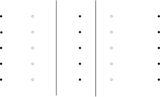
Figure 2: The charges and the conductors in $\log(s)$ plane. The original point-like charges are the small points between the conductors represented by the two lines. The others are the mirror images. There are $\pm 1$ point-like charges represented in distinct ways.

3.2.2 Multi-pronged string with one loop

To see how the quantization condition (3.6) appears, we shall construct the M2-brane configuration associated to a one-loop multi-pronged string the external strings of which stretch to infinity. In this case, the Riemann surface $\Sigma$ is a torus with some punctured points. The punctured points correspond to the ends of the infinitely stretching external strings. We parameterize $\Sigma$ with complex coordinate $u$ with identifications $u\sim u+1$ and $u\sim u+\tau_{\Sigma}$, where $\tau_{\Sigma}$ is the modular parameter of $\Sigma$. This curve is embedded in $Q=\{(s,t)\}$ with

$$s=s\,(u),~{}~{}t=t\,(u),$$ (3.13)

where $s\,(u)$ and $t\,(u)$ are some elliptic functions on the worldsheet torus $\Sigma$. From the definition of the parameters $s$ (2.9) and $t$ (2.10), we know that the punctured points correspond to the poles or zeros of the function $s\,(u)$ or $t\,(u)$.

Let us first discuss the function $s\,(u)$. Suppose the two-form charges of the infinitely stretching external strings are given by $(n_{e}^{a},n_{m}^{a})$ ($a=1,\cdots,n$). Then the end of a string with a positive $n_{e}^{a}$ should appear as an $n_{e}^{a}$-th order pole of $s$, while one with a negative $n_{e}^{a}$ as an $-n_{e}^{a}$-th order zero. Now suppose the ends are at $u=u_{a}$ on the torus $\Sigma$. Then, if and only if

$$\sum_{a=1}^{n}n_{e}^{a}u_{a}=-Q_{1}-Q_{2}\tau_{\Sigma}$$ (3.14)

with some integers $Q_{1}$ and $Q_{2}$, there exists an elliptic function with the above desired property:

$$s\,(u)=\exp(2(Q_{1}\eta_{1}+Q_{2}\eta_{3})u)\prod_{a=1}^{n}\sigma(u-u_{a})^{-n_{e}^{a}},$$ (3.15)

where the function $\sigma(u)$ is defined by

$$\sigma(u)=\exp(\eta_{1}u^{2})\theta_{1}(u|\tau_{\Sigma})/\theta_{1}^{\prime}(0|\tau_{\Sigma})$$ (3.16)

and $\eta_{1}=\sigma^{\prime}(1/2)/\sigma(1/2)$ and $\eta_{3}=\sigma^{\prime}(\tau_{\Sigma}/2)/\sigma(\tau_{\Sigma}/2)$.

The construction of the function $t\,(u)$ is similar. The following quantization condition must be satisfied by the charges $n_{m}^{i}$ and some integers $q_{1},q_{2}$:

$$\sum_{a=1}^{n}n_{m}^{a}u_{a}=-q_{1}-q_{2}\tau_{\Sigma}.$$ (3.17)

This equation gives further constraints on $u_{a}$. Then

$$t\,(u)=\exp(2(q_{1}\eta_{1}+q_{2}\eta_{3})u)\prod_{a=1}^{n}\sigma(u-u_{a})^{-n_{m}^{a}}.$$ (3.18)

There is a theorem that any two elliptic functions on a torus have an algebraic relation. Thus the torus coordinate $u$ can be eliminated, and the M2-brane configuration should be given by the zero locus of an algebraic function depending on the moduli of $\Sigma$:

$$f_{\Sigma}(s,t)=0.$$ (3.19)

To see what (3.14) means, we consider the line integral in fig. 3:

$$\oint_{C}\log(s)du = i(x^{10}(u+1)-x^{10}(u))\tau_{\Sigma}-i(x^{10}(u+\tau_{\Sigma})-x^{10}(u))$$ (3.20)

$$= 2\pi i(N_{1}\tau_{\Sigma}-N_{2}),$$

where the $N_{1}$ and $N_{2}$ are the electric fluxes crossing the two one-cycles of the torus, respectively. The other way to evaluate the integral is summing up the contributions from the zeros and poles of $s$:

$$-\oint_{C}ud(\log(s))=2\pi i\sum_{a=1}^{n}n_{e}^{a}u_{a}.$$ (3.21)

Thus (3.14) is just the quantization condition of the fluxes associated to the handles (3.6), and gives constraints on $u_{a}$.

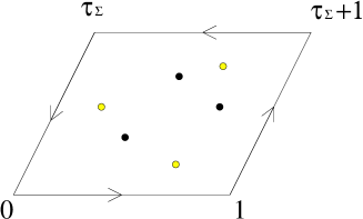
Figure 3: The closed contour $C$ in the $u$-plane. The small points are the zeros and poles of $s$.

We can also describe the conditions (3.14) and (3.17) graphically. Suppose that $u_{a}$ are in the fundamental region:

$$u_{a}=x_{a}+y_{a}\tau_{\Sigma},~{}~{}~{}~{}(\,0\leq x_{a},y_{a}\leq 1).$$ (3.22)

Then the conditions (3.14) and (3.17) become

$$\sum_{a=1}^{n}(n_{e}^{a},n_{m}^{a})\,x_{a}~{}\in\hbox{\mybb Z}^{2},$$ (3.23)

$$\sum_{a=1}^{n}(n_{e}^{a},n_{m}^{a})\,y_{a}~{}\in\hbox{\mybb Z}^{2}.$$ (3.24)

Since these two conditions are equivalent, it is enough to consider (3.23) only. We put the order of $x_{a}$ to satisfy $0\leq x_{1}\leq x_{2}\leq\cdots\leq x_{n}\leq 1$, and define

$$t_{1} = x_{1},$$ (3.25)

$$t_{i} = x_{i}-x_{i-1}~{}~{}~{}(i>1),$$ (3.26)

which satisfy $t_{i}\geq 0$ and $\sum_{i=1}^{n}t_{i}\leq 1$. We also define

$$(n^{i},m^{i})=\sum_{a=i}^{n}(n_{e}^{a},n_{m}^{a}),$$ (3.27)

with $i=1,\cdots,n$. Note that the charge conservation condition implies $(n^{1},m^{1})=(0,0)$. Then we can rewrite the condition (3.23) as

$$\sum_{i=1}^{n}(n^{i},m^{i})\,t_{i}~{}\in\hbox{\mybb Z}^{2},$$ (3.28)

which implies that there should exist a lattice point inside the convex hull of the vertices $(n^{i},m^{i})$. The condition (3.28) is most relaxed when $(n^{i},m^{i})$ become vertices of a convex polygon whose edges are given by the vectors $(n_{e}^{a},n_{m}^{a})$ as in fig.4.

Figure 4: The convex polygon whose edges are given by the vectors $(n_{e}^{a},n_{m}^{a})$.

Hence we conclude that the surface $\Sigma$ exists if and only if there is an integer lattice point inside the convex polygon whose edges are given by the vectors $(n_{e}^{a},n_{m}^{a})$. This condition is equivalent to that found in type IIB string theory using the grid diagrams [15, 18]. The modulus represented by the size of the loop diagram in string junction is now complexified and corresponds to the modular parameter $\tau_{\Sigma}$ in the M-theory description.

4 Physical interpretation in type IIA string theory

In the previous section, we used some technical methods in electrodynamics to find out holomorphic surface $\Sigma$ with given winding numbers $(n^{a}_{e},n^{a}_{m})$. The methods in electrodynamics was introduced with a purely mathematical motivation, and we did not care about the physical meaning.

In this section, we will try to make a physical interpretation of the methods and answer the question why the electrodynamics appeared in our problem. It turns out that there is a natural interpretation from the worldvolume gauge theory of D2-branes in the type IIA string theory.

Consider $n$ parallel D2-branes stretched along $x^{0},x^{5},x^{9}$ directions. We will use the static gauge

$$\sigma^{0}=x^{0},~{}\sigma^{1}=x^{5},~{}\sigma^{2}=x^{9},$$ (4.1)

where $(\sigma^{0},\sigma^{1},\sigma^{2})$ are the worldvolume coordinates of the D2-branes. The effective worldvolume theory is 3-dim $U(n)$ SYM which is obtained by dimensional reduction of 10-dim ${\cal N}=1$ $U(n)$ SYM. The bosonic part of the action is

$$S=T\int d^{3}\sigma\mathop{\rm Tr}\nolimits\left(-\frac{1}{4}F_{\mu\nu}F^{\mu\nu}+\frac{1}{2}D_{\mu}X^{I}D^{\mu}X^{I}+\frac{1}{4}[X^{I},X^{J}]^{2}\right),$$ (4.2)

where $T$ is the D2-brane tension, and $X^{I}$ $(I=1,\cdots,4,6,\cdots,8)$ are adjoint scalar fields, which represent the transverse fluctuations of the D2-branes.

Let us consider the BPS configuration of this system. The energy is expressed as

$$U=\frac{\,T\,}{2}\int d^{2}\sigma\mathop{\rm Tr}\nolimits\left(\vec{E}^{2}+B^{2}+(D_{0}X^{I})^{2}+(\vec{D}X^{I})^{2}-\frac{1}{2}[X^{I},X^{J}]^{2}\right),$$ (4.3)

where we have assumed that the fermion fields are zero. Here we have defined electric and magnetic fields in 3-dim as

$$\vec{E} = (E_{1},E_{2})=(F_{01},F_{02}),$$ (4.4)

$$B = F_{12}.$$ (4.5)

Introducing a unit vector $\eta^{I}$ in $\hbox{\mybb R}^{7}$, we have

$$U=\frac{\,T\,}{2}\int d^{2}\sigma\mathop{\rm Tr}\nolimits\left(\,\left|\,\eta^{I}\vec{E}-\vec{D}X^{I}\,\right|^{2}+B^{2}+(D_{0}X^{I})^{2}-\frac{1}{2}[X^{I},X^{J}]^{2}+2\eta^{I}\vec{E}\cdot\vec{D}X^{I}\right).$$ (4.6)

Since the first four terms in the parenthesis in (4.6) are positive definite, we obtain a bound for the energy

$$U\geq T\,\eta^{I}\,Q_{E}^{I},$$ (4.7)

where we have defined the charge vector

$$Q_{E}^{I} = \int d^{3}\sigma\mathop{\rm Tr}\nolimits\left(\vec{E}\cdot\vec{D}X^{I}\right)$$ (4.8)

$$= \int_{S^{1}_{\infty}}d\vec{S}\cdot\mathop{\rm Tr}\nolimits\left(\vec{E}X^{I}\right).$$ (4.9)

Here we have used the Gauss’s Law in the last equality.

The right hand side of (4.7) is maximized when $\eta^{I}$ is proportional to the charge vector $Q^{I}_{E}$, and then we obtain the Bogomol’nyi bound

$$U\geq T\,\|\,Q_{E}^{I}\|.$$ (4.10)

The BPS configurations, which saturate this bound, satisfy the following equations:

$$\eta^{I}\vec{E}=\vec{D}X^{I},~{}~{}B=0,~{}~{}D_{0}X^{I}=0,~{}~{}[X^{I},X^{J}]=0.$$ (4.11)

Now consider the M-theory description of the D2-brane configurations. We consider the case with a single D2-brane ($n=1$ case). As shown in [19, 20, 21], the M2-brane action can be obtained by performing a duality transformation of a worldvolume gauge field in the D2-brane action. The scalar field corresponding to the fluctuations of the M2-brane in $x^{10}$ direction is the dual of the worldvolume gauge field on the D2-brane:

$$F^{\mu\nu}=\epsilon^{\mu\nu\rho}\,\partial_{\rho}X^{10}.$$ (4.12)

Let us assume $X^{I}=0$ for $I=1,2,3,6,7,8$ as in the previous sections. The BPS configurations (4.11) are static configurations satisfying

$$E_{i}=\partial_{i}X^{4},~{}~{}B=0.$$ (4.13)

Hence, using (4.12), we obtain

$$\epsilon_{0ij}\,\partial_{j}X^{10} = \partial_{i}X^{4},$$ (4.14)

$$\partial_{0}X^{10} = 0.$$ (4.15)

(4.14), together with (4.1), is nothing but the Cauchy-Riemann equation

$$\frac{\partial X^{4}}{\partial x_{5}}=\frac{\partial X^{10}}{\partial x_{9}},~{}~{}~{}\frac{\partial X^{4}}{\partial x_{9}}=-\frac{\partial X^{10}}{\partial x_{5}},$$ (4.16)

which imply that the M2-brane is holomorphically embedded in $Q$, as explained in section 2.

In the previous section, we interpreted $X^{4}$ as the scalar potential and the winding number $n_{e}^{a}$ on the boundary of the membrane in $x^{10}$ direction as the electric charge in the 3-dim electrodynamics. Now it is clear from (4.13) and (4.12) that these interpretations can be naturally understood from the electrodynamics of the D2-brane worldvolume gauge theory.

Acknowledgments
We would like to thank K. Hashimoto, H. Hata and T. Kugo for valuable discussions. We would like to thank also the organizers of the Summer Institute ‘98, where we began the present work. N.S. is Supported in part by Grant-in-Aid for Scientific Research from Ministry of Education, Science and Culture (#09640346) and Priority Area: “Supersymmetry and Unified Theory of Elementary Particles” (#707). S.S. is supported in part by Grant-in-Aid for JSPS fellows.

References

- [1] E. Witten, Nucl. Phys. B460 (1996) 335, hep-th/9510135.
- [2] A.A. Tseytlin, Nucl. Phys. B469 (1996) 51, hep-th/9602064; M.B. Green and M. Gutperle, Phys. Lett. B377 (1996) 28, hep-th/9602077.
- [3] C. Montonen and D. Olive, Phys. Lett. B72 (1977) 117.
- [4] J.H. Schwarz, Nucl. Phys. Proc. Suppl. 55B (1997) 1, hep-th/9607201; O. Aharony, J. Sonnenschein and S. Yankielowicz, Nucl. Phys. B474 (1996) 309, hep-th/9603009.
- [5] O. Bergman, Nucl. Phys. B525 (1998) 104, hep-th/9712211.
- [6] K. Hashimoto, H. Hata and N. Sasakura, Phys. Lett. B431 (1998) 303, hep-th/9803127; hep-th/9804164.
- [7] T. Kawano and K. Okuyama, Phys. Lett. B432 (1998) 338, hep-th/9804139; K. Lee and P. Yi, Phys. Rev. D58 (1998) 066005, hep-th/9804174.
- [8] N. Seiberg and E. Witten, Nucl. Phys. B426 (1994) 19, hep-th/9407087; Nucl. Phys. B431 (1994) 484, hep-th/9408099.
- [9] E. Witten, Nucl. Phys. B500 (1997) 3, hep-th/9703166.
- [10] M. Krogh and S. Lee, Nucl. Phys. B516 (1998) 241, hep-th/9712050; Y. Matsuo and K. Okuyama, Phys. Lett. B426 (1998) 294, hep-th/9712070; I. Kishimoto and N. Sasakura, Phys. Lett. B432 (1998) 305, hep-th/9712180.
- [11] B. Kol, hep-th/9705031; O. Aharony, A. Hanany and B. Kol, J. High Energy Phys. 01 (1998) 002, hep-th/9710116.
- [12] A. Fayyazuddin and M. Spalinski, Nucl. Phys. B508 (1997) 219, hep-th/9706087.
- [13] M. Henningson and P. Yi, Phys. Rev. D57 (1998) 1291, hep-th/9707251.
- [14] A. Mikhailov, Nucl. Phys. B533 (1998) 243, hep-th/9708068.
- [15] A. Mikhailov, N. Nekrasov and S. Sethi, Nucl. Phys. B531 (1998) 345, hep-th/9803142.
- [16] S. Sugimoto, Prog. Theor. Phys. 100 (1998) 123, hep-th/9804114.
- [17] C. Fraser and T. Hollowood, Phys. Lett. B402 (1997) 106, hep-th/9704011.
- [18] O. Bergman and B. Kol, hep-th/9804160.
- [19] P.K. Townsend, Phys. Lett. B373 (1996) 68, hep-th/9512062.
- [20] E. Bergshoeff and P.K. Townsend, Nucl. Phys. B490 (1998) 145, hep-th/9611173.
- [21] M. Aganagic, J. Park, C. Popescu, and J.H. Schwarz, Nucl. Phys. B496 (1997) 215, hep-th/9702133.
- [22] See for example, O. Forster, “Lectures on Riemann Surfaces”, Springer-Verlag.