Low Energy States in the $SU(N)$ Skyrme Models DTP98/51    UKC98/42

Abstract

We show that any solution of the $SU(2)$ Skyrme model can be used to give a topologically trivial solution of the $SU(4)$ one. In addition, we extend the method introduced in [1] and use harmonic maps from $S^{2}$ to $CP^{(N-1)}$ to construct low energy configurations of the $SU(N)$ Skyrme models. We show that one of such maps gives an exact, topologically trivial, solution of the $SU(3)$ model. We study various properties of these maps and show that, in general, their energies are only marginally higher than the energies of the corresponding $SU(2)$ embeddings. Moreover, we show that the baryon (and energy) densities of the $SU(3)$ configurations with baryon number $B=2-4$ are more symmetrical than their $SU(2)$ analogues. We also present the baryon densities for the $B=5$ and $B=6$ configurations and discuss their symmetries.

1 INTRODUCTION

The Skyrme model is now well established as an effective classical theory used to describe nuclei [2, 3] for which the field, which describes pions, is valued in $SU(N)$. To have finite energy configurations, one must require that the field $U(\vec{x},t)$ goes to a constant matrix, say $I$, at spatial infinity: $U\rightarrow I$ as $|\vec{x}|\rightarrow\infty$. This effectively compactifies the three dimensional Euclidean space into $S^{3}$ and hence implies that the field configurations of the Skyrme model can be considered as mappings from $S^{3}$ into $SU(N)$.

In terms of the algebra valued currents $\partial_{\mu}U\,U^{-1}$, the Lagrangian is,

$${\cal L}=\frac{F^{2}}{16}\,\mbox{tr}\left(\partial_{\mu}U\,\partial^{\mu}U^{-1}\right)+\frac{1}{32a^{2}}\,\mbox{tr}\left[\partial_{\mu}U\,U^{-1},\partial_{\nu}U\,U^{-1}\right]^{2},$$ (1)

where $U(\vec{x},t)$ is an $SU(N)$ valued scalar field, $F\approx 189$ MeV is the pion decay constant and $a$ is a dimensional constant.

The last term, called the Skyrme term, stabilises the solitons and, in addition, introduces small interaction forces between them. Their nature depends on the relative orientation of skyrmions in their internal space. If we want to study interactions of physical mesons we have to introduce further terms which are responsible for the meson masses, ie terms of the form

$${\cal L}_{m}=\frac{F^{2}}{16}\,M_{\pi}^{2}\,\mbox{tr}\left(U^{-1}+U-2\,{\it I}\right).$$ (2)

Such terms play a more significant role in lower dimensions since in (2+1) dimensions their presence, together with the Skyrme term, is required to stabilise the solitons. However, in (3+1) dimensions the solitons are stable even when $M_{\pi}=0$. In what follows, we will set $M_{\pi}=0$ except in section 5.

In this paper, we concentrate our attention on studying the static properties of the model and we consider $U(\vec{x})$ fields, which are stationary points of the energy functional. After rescaling the space-time coordinates [4, 5] $\vec{x}\rightarrow{2\vec{x}/aF}$ and defining $m_{\pi}=M_{\pi}{2/aF}$, we can write the static energy corresponding to the lagrangian (1) and (2) as

$$E={F\over 4a}\int_{R^{3}}\left\{-\frac{1}{2}\,\mbox{tr}\left(\partial_{i}U\,U^{-1}\right)^{2}-\frac{1}{16}\,\mbox{tr}\left[\partial_{i}U\,U^{-1},\partial_{j}U\,U^{-1}\right]^{2}-{m_{\pi}^{2}\over 2}\mbox{tr}(U^{-1}+U-2\,{\it I})\right\}d^{3}\vec{x}.$$ (3)

From now on, we will take $F/4a=1/12\pi^{2}$ so that the energy is expressed in the same units as the baryon number. In this case, the static fields $U$ obey the equation

$$\partial_{i}\left(\partial_{i}U\,U^{-1}-\frac{1}{4}\,[\partial_{j}U\,U^{-1},[\partial_{j}U\,U^{-1},\partial_{i}U\,U^{-1}]]\right)-\frac{m_{\pi}^{2}}{4}\left(U-U^{-1}\right)=0.$$ (4)

As the third homotopy class of $SU(N)$ is $Z$ every field configuration is characterised by an integer:

$$B=\frac{1}{24\pi^{2}}\int_{R^{3}}\varepsilon_{ijk}\,\mbox{tr}\left(\partial_{i}U\,U^{-1}\partial_{j}U\,U^{-1}\partial_{k}U\,U^{-1}\right)d^{3}\vec{x},$$ (5)

which is to be interpreted as the baryon number [3, 6]; therefore, the lowest energy state in the $B=1$ sector can be identified with the (classical) nucleon.

So far most of the studies involving the Skyrme model have concentrated on the $SU(2)$ version of the model and its embeddings into $SU(N)$. The simplest nontrivial classical solution involves a single skyrmion ($B=1$) and has already been discussed by Skyrme [2]. The energy density of this solution is radially symmetric and, as a result, using the so-called hedgehog ansatz one can reduce (4) to an ordinary differential equation which can then be solved numerically.

Many solutions with $B>1$ have also been computed numerically and in all cases the solutions are very symmetrical (cf. Battye et al. [5] and references therein). The energy density of the two skyrmion solution forms a torus, while the energy density of the $B=3$ solution has the symmetry of a tetrahedron. For larger $B$ the solutions describe semi-radially symmetric structures in which skyrmions break up into connected parts which are all located on a spherical hollow shell and, as was shown in [1], the positions of these skyrmionic parts on $S^{2}$ are very symmetrical.

Recently, Houghton et al. [1] have showed that by using rational maps from $S^{2}$ to $S^{2}$ one can easily construct field configurations for the $SU(2)$ model which are close to being solutions of the model: they have energies slightly higher than the energies of the exact solutions found numerically but the symmetries of the baryon and energy densities are the same. When these configurations are used as initial conditions in a relaxation program, the fields do not change much as they evolve towards the exact solutions.

All this work has involved the $SU(2)$ skyrmions; however, so far, very little has been done for the $SU(N)$ model when $N>2$. An interesting question then arises as to whether there are any finite energy solutions of the $SU(N)$ ($N>2$) model which are not embeddings of the $SU(2)$ model and, if they exist, whether they have lower energies than their $SU(2)$ counterparts.

The first example of such a non-embedding configuration for a higher group was the $SO(3)$ soliton, which corresponds to a bound system of two skyrmions, and which was found using the chiral field ansatz by Balachandran et al. [7]. Another configuration, with a large $SU(3)$ strangeness content, was found by Kopeliovich et al. [8]. However, all other known skyrmion configurations seem to have been the embeddings of the solutions of the $SU(2)$ model.

2 $SU(2)$ EMBEDDINGS

As we have said before, any solution of the $SU(N^{\prime})$ model is automatically a solution of any $SU(N)$ model as long as $N^{\prime}<N$; simply by completing the entries of the larger matrix with 1’s along the diagonal and 0’s off diagonal. The energy, the baryon number and all other properties are unchanged by this operation and so such embeddings have the same properties as the original fields.

However, there exist further, less obvious embeddings in which new fields have different properties from the original ones. In particular, one can show that any solution of the $SU(2)$ model generates a solution of the $SU(4)$ one.

A special feature of the $SU(2)$ field is that it can be written as

$$U=\vec{\phi}\,\vec{\tau},$$ (6)

where $\vec{\tau}=(1,i\sigma_{1},i\sigma_{2},i\sigma_{3})$ and the $\sigma$’s stand for the Pauli matrices. The unitarity of $U$ requires that $\vec{\phi}\cdot\vec{\phi}=1$; and the energy density of this $SU(2)$ field is

$${\cal E}_{2}=\,(\partial_{i}\vec{\phi}\cdot\partial_{i}\vec{\phi})+\frac{1}{2}\left[(\partial_{i}\vec{\phi}\cdot\partial_{i}\vec{\phi})^{2}-(\partial_{i}\vec{\phi}\cdot\partial_{j}\vec{\phi})^{2}\right].$$ (7)

Moreover, the equations of motion which follow from (4) are

$$\vec{\phi}_{ii}+\vec{\phi}_{ii}\,(\vec{\phi}_{j}\cdot\vec{\phi}_{j})+\,\vec{\phi}_{i}\,(\vec{\phi}_{ij}\cdot\vec{\phi}_{j})-\vec{\phi}_{ij}\,(\vec{\phi}_{i}\cdot\vec{\phi}_{j})-\vec{\phi}_{j}\,(\vec{\phi}_{ii}\cdot\vec{\phi}_{j})-\vec{\phi}\,(\vec{\phi}\cdot\vec{\phi}_{ii})$$

$$-\vec{\phi}\left[(\vec{\phi}\cdot\vec{\phi}_{ii})\,(\vec{\phi}_{j}\cdot\vec{\phi}_{j})-(\vec{\phi}\cdot\vec{\phi}_{ij})\,(\vec{\phi}_{i}\cdot\vec{\phi}_{j})\right]=0,$$ (8)

where $\vec{\phi}_{i}=\partial_{i}\vec{\phi}$ and $\vec{\phi}_{ij}=\partial_{ij}\vec{\phi}$.

Notice now that we can construct an $SU(4)$ field out of any $S^{3}$ field $\vec{\phi}$ by taking

$$U=U_{0}\,\left({\it I}-2\,\vec{\phi}\otimes\vec{\phi}\,^{\dagger}\right),$$ (9)

where $U_{0}$ is a constant matrix. Note that $\det U=-\det U_{0}$ and so by choosing $U_{0}$ to be a constant matrix of determinant -1 we see that $U$ is unitary. In this case, $U^{-1}=({\it I}-2\,\vec{\phi}\otimes\vec{\phi}\,^{\dagger})\,U_{0}^{-1}$ and the $U_{0}$’s cancel in (4).

To derive the equation that the field $\vec{\phi}$ must satisfy so that (9) is a solution of (4), with $m_{\pi}=0$, we note that the condition $\vec{\phi}\cdot\vec{\phi}=1$ gives

$$\partial_{j}UU^{-1}\,=\,2\,\partial_{j}\vec{\phi}\otimes\vec{\phi}^{\dagger}\,-\,2\,\vec{\phi}\otimes\partial_{j}\vec{\phi}^{\dagger},$$ (10)

and so (4) becomes

$$\!\!\!\!\!\!\!\!\!\!\!\!\!\!2\partial_{i}\left[\vec{\phi}\otimes\partial_{j}\vec{\phi}^{\dagger}\left(\partial_{j}\vec{\phi}\cdot\partial_{i}\vec{\phi}\right)\!-\!\vec{\phi}\otimes\partial_{i}\vec{\phi}^{\dagger}\left(\partial_{j}\vec{\phi}\cdot\partial_{j}\vec{\phi}\right)\!+\!\partial_{i}\vec{\phi}\otimes\vec{\phi}^{\dagger}\left(\partial_{j}\vec{\phi}\cdot\partial_{j}\vec{\phi}\right)\!-\!\partial_{j}\vec{\phi}\otimes\vec{\phi}^{\dagger}\left(\partial_{i}\vec{\phi}\cdot\partial_{j}\vec{\phi}\right)\right]$$

$$\hskip 287.37283pt+\partial_{i}\left(\partial_{i}\vec{\phi}\otimes\vec{\phi}^{\dagger}-\vec{\phi}\otimes\partial_{i}\vec{\phi}^{\dagger}\right)=0.$$

(11)

One can easily show that the equations (11) and (8) are equivalent, implying that $\vec{\phi}$ satisfies the equation of the $SU(2)$ Skyrme model (11). We can thus conclude that any solution of the $SU(2)$ model can be transformed into a solution of the $SU(4)$ model by the embedding (9).

The solutions obtained this way are topologically trivial since their baryon density vanishes identically. Moreover, their energy density is

$${\cal E}_{3}=4\,(\partial_{i}\vec{\phi}\cdot\partial_{i}\vec{\phi})+2\left[(\partial_{i}\vec{\phi}\cdot\partial_{i}\vec{\phi})^{2}-(\partial_{i}\vec{\phi}\cdot\partial_{j}\vec{\phi})^{2}\right],$$ (12)

ie it is four times larger than the corresponding energy of the original $SU(2)$ field (7).

This suggests that these particular $SU(4)$ solutions may be interpreted as states corresponding to $2B$ skyrmions and $2B$ anti-skyrmions, where $B$ is the baryon number of the original $SU(2)$ solution. Incidentally, a similar situation arises in 2-dimensions where any $B$ solitonic solution of the $CP^{1}$ model gives a topologically trivial solution of the $CP^{2}$ model which can be interpreted as a bound state of $2B$ solitons and $2B$ anti-solitons [9].

3 HARMONIC MAPS ANSATZ

Recently, Houghton et al. [1] exploited the similarity of the energy densities of the multi-skyrmion solutions to those of the $SU(2)$ BPS monopoles and presented a new ansatz for constructing $SU(2)$ multi-skyrmion fields; based on rational maps of the two dimensional sphere $S^{2}$. Namely, they showed that solutions of the Skyrme model can be well approximated by the expressions of the form

$$U(r,\theta,\phi)=\exp(ig(r)\,\mbox{\boldmath$\hat{n}\cdot\sigma$}),$$ (13)

where $(r,\theta,\phi)$ are the usual polar coordinates on $\bf R^{3}$, and

$$\mbox{\boldmath$\hat{n}$}={1\over 1+|R|^{2}}(2\Re(R),2\Im(R),1-|R|^{2}),$$ (14)

where $R$ are rational functions of $\xi=\tan(\theta/2)e^{i\phi}$ and where $g(r)$ is a real function satisfying the boundary conditions: $g(0)=\pi$ and $g(\infty)=0$. In other words, the configuration (13) involves a radial profile function $g(r)$ and a rational map from the two dimensional sphere of radius $r$ which can be identified with a sphere centered at the origin, in ${\bf R^{3}}$, into a $S^{2}$ submanifold of $SU(2)\equiv S^{3}$. Moreover, it is easy to check that the baryon number $B$ is given by the degree of the rational map $\hat{n}$.

To determine $g$ and $\hat{n}$ one must insert (13) into (3) and minimise the energy. It turns out that, for this minimum, $\hat{n}$ must be a rational map with a large discrete symmetry and that $g(r)$ satisfies an ordinary differential equation.

In this section we show that this idea of Houghton et al. can be generalised to $SU(N)$. Using the polar coordinates $(r,\theta,\phi)$ in ${\bf R^{3}}$, our generalisation of Houghton et al.’s ansatz is to consider $U$ of the form

$$U(r,\theta,\phi) = e^{2ig(r)(P-{\it I}/N)}$$ (15)

$$= e^{-2ig(r)/N}\left({\it I}+(e^{2ig}-1)P\right),$$

where $P$ is a $N\times N$ hermitian projector which depends only on the angular variables $(\theta,\phi)$ and $g(r)$ is the radial profile function. Note that, the matrix $P$ can be thought of as a mapping from $S^{2}$ into $CP^{(N-1)}$. Hence it is convenient, rather than using the polar coordinates, to map the sphere onto the complex plane via a stereographic projection and, instead of $\theta$ and $\phi$, use the complex coordinate $\xi$ and its conjugate. Thus, $P$ can be written as

$$P(V)=\frac{V\otimes V^{\dagger}}{|V|^{2}},$$ (16)

where $V$ is a $N$ component complex vector (dependent on $\xi$ and $\bar{\xi}$).

For (15) to be well-defined at the origin, like (13), the radial profile function $g(r)$ has to satisfy $g(0)=\pi$ while the boundary value $U\rightarrow I$ at $r=\infty$ requires that $g(\infty)=0$. An attractive feature of the ansatz (15) is that it leads to a simple expression for the energy density which can be successively minimized with respect to the parameters of the projector $P$ and then with respect to the shape of the profile function $g(r)$. This is then expected to give good approximations to multi-skyrmion field configurations.

Moreover, we will show that this method not only allows us to find such field configurations but also gives us an exact non-topological solution of the $SU(3)$ Skyrme model. We will also present some upper bounds on the energy of some multi-skyrmion field configurations in the $SU(N)$ model (with radially symmetric energy density distribution). In what follows, we restrict our attention to the case $m_{\pi}=0$.

To find the exact solution of the $SU(3)$ model we put (15) into (4) and obtain

$$\!\!\!\!\!\!\!\!-\frac{2i}{r^{2}}\,\partial_{r}(g_{r}\,r^{2})\,(\frac{{\it I}}{N}-P)-\frac{i}{2r^{2}}\,\partial_{r}(g_{r}|A|^{2})\,(1+|\xi|^{2})^{2}\left([P_{\bar{\xi}},P\,P_{\xi}]+[P_{\xi},P\,P_{\bar{\xi}}]\right)\!$$

$$\!\!\!\!\!\!\!\!+\frac{\bar{A}|A|^{2}}{16r^{4}}(1+|\xi|^{2})^{2}\left\{\partial_{\bar{\xi}}\left((1+|\xi|^{2})^{2}[P_{\xi},[P_{\bar{\xi}},P_{\xi}]]\right)\!-\!\partial_{{\xi}}\left((1+|\xi|^{2})^{2}[P_{\bar{\xi}},[P_{\bar{\xi}},P_{\xi}]]\right)\right\}\!$$

$$\!\!\!\!\!\!\!\!+\frac{|A|^{4}}{16r^{4}}(1\!+\!|\xi|^{2})^{2}\left\{\partial_{\bar{\xi}}\left((1\!+\!|\xi|^{2})^{2}[P_{\xi}P,[P_{\bar{\xi}},P_{\xi}]]\right)\!-\!\partial_{{\xi}}\left((1\!+\!|\xi|^{2})^{2}[P_{\bar{\xi}}P,[P_{\bar{\xi}},P_{\xi}]]\right)\right\}$$

$$\!\!\!\!\!\!\!\!+\frac{1}{r^{2}}(1+g^{2}_{r})(1+|\xi|^{2})^{2}\left[\bar{A}\,P_{\xi\bar{\xi}}+\frac{|A|^{2}}{2}\left(\partial_{\xi}(P_{\bar{\xi}}\,P)+\partial_{\bar{\xi}}(P_{\xi}\,P)\right)\right]=0,$$ (17)

where $A=e^{-2ig}-1$.

Moreover, the energy (3) simplifies to

$$E={1\over 3\pi}\int dr\left(A_{N}\,g_{r}^{2}\,r^{2}+2{\cal N}\,\sin^{2}g\,(1+g_{r}^{2})+{\cal I}\,\frac{\sin^{4}g}{r^{2}}\right),$$ (18)

where

$$A_{N} = \frac{2}{N}(N-1),$$ (19)

$${\cal N} = \frac{i}{2\pi}\int d\xi\,d\bar{\xi}\,\mbox{tr}\left(|\partial_{\xi}P|^{2}\right),$$ (20)

$${\cal I} = \frac{i}{4\pi}\int d\xi\,d\bar{\xi}\,(1+|\xi|^{2})^{2}\,\mbox{tr}\left([\partial_{\xi}P,\,\partial_{\bar{\xi}}P]^{2}\right).$$ (21)

As the integrals ${\cal N}$ and ${\cal I}$ in (18) are independent of $r$, we can minimise (18) by first minimising ${\cal N}$ and ${\cal I}$ as functions of $P$ and then with respect to the profile function $g$.

However, since ${\cal N}$ is the expression for the energy of the two dimensional Euclidean $CP^{2}$ sigma model, all classical solutions contain the so-called self-dual solutions, instantons or holomorphic maps from $S^{2}$ into $CP^{(N-1)}$, first given in [11], which are given by the projector $P$ of the form (16) with $V=f(\xi)$. In this case, the energy $\cal{N}$ is given by the degree of $f$, ie the degree of the highest order polynomial in $\xi$ among the components of $f$ after all their common factors have been canceled.

By a Bogomolny-type argument it can be shown that

$$E \!\!\!\!\!\!\!\!={1\over 3\pi}\!\!\int\!dr\left[\left(g_{r}r\sqrt{A_{N}}+\sqrt{{\cal I}}\,\frac{\sin^{2}g}{r}\right)^{2}+2N\sin^{2}g\,(1+g_{r})^{2}-2g_{r}\,\sin^{2}g\left(2N+\sqrt{A_{N}\,{\cal I}}\right)\,\right]$$ (22)

$$\!\!\!\!\!\!\!\!\geq{1\over 3}\,\left(2\,N+\sqrt{A_{N}\,{\cal I}}\,\,\right).$$

Finally, the baryon number for this ansatz is given by

$$B = \frac{i}{\pi^{2}}\int d\xi\,d\bar{\xi}\,\mbox{tr}\left(P\,[\partial_{\xi}P,\,\partial_{\bar{\xi}}P]\right)\int_{0}^{\infty}dr\,\sin^{2}g\,g_{r}\,$$ (23)

$$= \frac{i}{2\pi}\int d\xi\,d\bar{\xi}\,\mbox{tr}\left(P\,[\partial_{\bar{\xi}}P,\,\partial_{\xi}P]\right),$$

which is the topological charge of the two-dimensional $CP^{(N-1)}$ sigma model.

In the next two sections we will show that this ansatz gives us interesting low energy field configurations of the $SU(N)$ Skyrme model which are not the $SU(2)$ embeddings. To minimise $E$ we will, first of all, fix the baryon number ${\cal N}=B$ of the configurations we are interested in. We will then minimise ${\cal I}$ over all maps of degree $B$ and then derive a second order differential equation for $g$ by minimising the energy (18) treating ${\cal N}$ and ${\cal I}$ as parameters.

4 $SU(3)$ EXACT SOLUTION

When the projector $P$ is analytic, ie is of the form

$$P_{0}=P(f)=\frac{f\,f^{\dagger}}{|f|^{2}},$$ (24)

where $f$ is a holomorphic vector (ie whose entries are functions only of $\xi$) then it satisfies the equation

$$P_{0}\,\partial_{\xi}P_{0}=0,\hskip 14.22636pt\hskip 14.22636pt\hskip 14.22636pt\partial_{\xi}P_{0}\,P_{0}=\partial_{\xi}P_{0},$$ (25)

ie the self-dual equations of the two dimensional $CP^{(N-1)}$ sigma models [9].

Following [10], we define the operator $P_{+}$ by its action on any vector $v\in{\rm C}^{N}$ as

$$P_{+}v=\partial_{\xi}v-\frac{v\,(v^{\dagger}\,\partial_{\xi}v)}{|v|^{2}},$$ (26)

and then define further vectors $P^{k}_{+}v$ by induction: $P^{k}_{+}v=P_{+}(P^{k-1}_{+}v)$.

To proceed further we note the following useful properties of $P^{k}_{+}f$ when $f$ is holomorphic:

$$(P^{k}_{+}f)^{\dagger}\,P^{l}_{+}f=0,\hskip 14.22636pt\hskip 14.22636pt\hskip 14.22636ptk\neq l,$$ (27)

$$\partial_{\bar{\xi}}\left(P^{k}_{+}f\right)=-P^{k-1}_{+}f\frac{|P^{k}_{+}f|^{2}}{|P^{k-1}_{+}f|^{2}},\hskip 14.22636pt\hskip 14.22636pt\partial_{\xi}\left(\frac{P^{k-1}_{+}f}{|P^{k-1}_{+}f|^{2}}\right)=\frac{P^{k}_{+}f}{|P^{k-1}_{+}f|^{2}}.$$ (28)

These properties either follow directly from the definition of the $P_{+}$ operator or are very easy to prove [9].

It is also convenient to define projectors corresponding to the family of $P_{+}^{k}f$ vectors as follows:

$$P_{0}=P(f),\hskip 14.22636pt\hskip 14.22636ptP_{1}=P(P_{+}f),\hskip 14.22636pt\hskip 14.22636pt\dots,\hskip 14.22636pt\hskip 14.22636ptP_{i}=P(P^{i}_{+}f).$$ (29)

Taking $P=P_{i}$, for given $i$, and using the above properties we observe that all the terms in (17), except the first one, can be gathered into one term if and only if

$$\frac{|P_{+}f|^{2}}{|f|^{2}}\equiv\frac{{\cal K}}{(1+|\xi|^{2})^{2}},$$ (30)

where ${\cal K}$ is a constant. Moreover, for the $SU(2)$ case, the projectors $P_{0}$ and $P_{1}$ satisfy the relation

$$P_{0}+P_{1}={\it I},$$ (31)

and for $f=(1,\xi)$ all the terms in (17) are proportional to one common matrix thus giving a second order differential equation for the profile function $g$. This means that the Skyrme field (15), in the case when $g$ satisfies its equation, is an exact solution of the equation (17). A little thought shows that this is the well known hedgehog solution.

Unfortunately this discussion does not generalise to higher $SU(N)$ groups. However, we note that for the $SU(3)$ model, if we take $P=P_{1}$ and use the fact that $P_{0}+P_{1}+P_{2}={\it I}$, all the matrix terms in equation (17) become proportional to each other leading to a second order differential equation for the profile function, if and only if

$$\frac{|P_{+}^{2}f|^{2}}{|P_{+}f|^{2}}+\frac{|P_{+}f|^{2}}{|f|^{2}}\equiv\frac{\tilde{\cal K}}{(1+|\xi^{2}|)^{2}},$$ (32)

where $\tilde{\cal K}$ is a constant. This last condition is satisfied if

$$f=(1,\,\sqrt{2}\,\xi,\,\xi^{2})^{t}.$$ (33)

Thus, by taking $P=P_{1}$ for $f$ of the form (33), and requiring $g$ to satisfy the equation

$$g_{rr}\left(\frac{1}{3}+2\,\frac{\sin^{2}g}{r^{2}}\right)+\frac{2}{3}\,\frac{g_{r}}{r}+\frac{\sin 2g}{r^{2}}\left(g_{r}^{2}-1-\frac{\sin^{2}g}{r^{2}}\right)=0,$$ (34)

we see that (15) is an exact solution of the $SU(3)$ model.

For this solution, the parameters in the energy density can be evaluated analytically; we find

$$A_{N}=\frac{4}{3},\hskip 14.22636pt\hskip 14.22636pt{\cal N}=4,\hskip 14.22636pt\hskip 14.22636pt{\cal I}=4,$$ (35)

and the total energy is $E=3.861$.

To understand what this solution corresponds to we calculate the topological charge of this configuration and find

$$B=\frac{i}{\pi}\int d\xi\,d\bar{\xi}\,\left(\frac{|P^{2}_{+}f|^{2}}{|f|^{2}}-\frac{|P_{+}f|^{2}}{|f|^{2}}\right),$$ (36)

which due to the conditions (27), (28) and (32) is identically zero.

Although the baryon density is identically zero the solution itself is nontrivial. This follows from the fact that the $CP^{2}$ sigma model harmonic map $P_{1}$ corresponds to a mixture of two solitons and two anti-solitons. Thus it seems reasonable to interpret this solution as describing a bound state of two skyrmions and two anti-skyrmions and as such to be unstable, ie correspond to a saddle point of the energy. However, let us emphasize, once again, that this field configuration is a genuine solution of the $SU(3)$ Skyrme model.

It is easy to see that this new field configuration has an energy density distribution shaped like a shell (ie is radially symmetric). To see this note that for this solution, $\mbox{tr}\left(|\partial_{\xi}P|^{2}\right)$ and $\mbox{tr}\left([\partial_{\xi}P,\partial_{\bar{\xi}}P]^{2}\right)$ which appear in (20) and (21), are proportional to $(1+|\xi|^{2})^{-2}$ and $(1+|\xi|^{2})^{-4}$, respectively; demonstrating this symmetry. The radial energy density of this solution is given in Figure 1 and one sees that it corresponds to a hollow ball.

Figure 1: Energy profile of the non-topological solution.

5 APPROXIMATE RADIALLY SYMMETRIC SKYRME FIELDS

What about further genuine solutions? In general, our method does not give us further solutions but it is a matter of simple algebra to show that the condition (30) is true for any $N\geq 2$ when the modulus of the vector $f$ is some power of $(1+|\xi|^{2})$. In fact, we have

$$N=2, f=(1,\xi)^{t},$$ (37)

$$N=3, f=(1,\sqrt{2}\xi,\xi^{2})^{t},$$ (38)

$$N=4, f=(1,\sqrt{3}\xi,\sqrt{3}\xi^{2},\xi^{3})^{t},$$ (39)

$$N=n, f=(f_{0},f_{1},\dots,f_{n-1})^{t}:\hskip 14.22636ptf_{i}=\xi^{i}\sqrt{C_{i+1}^{n-1}},$$ (40)

where $C_{i+1}^{n-1}$ denotes the binomial coefficients. Note that in this case, the constant ${\cal K}$ in (30) is equal to the degree of the vector $f$: ie ${\cal K}=n$.

Using the condition (30) the integrals involving $P$ in the energy (18) can be evaluated analytically,

$${\cal N}=n,\hskip 14.22636pt\hskip 14.22636pt{\cal I}=(N-1)^{2}=n^{2}.$$ (41)

Using the analyticity of the projector $P_{0}$, it is straightforward to verify that the baryon number of this field is $B=n$, ie the degree of $f$.

When $m_{\pi}\neq 0$ the energy (18) for the ansatz (15) becomes

$$E\!\!\! = \!\!\!{1\over 3\pi}\!\int\!dr\{A_{N}\,g_{r}^{2}\,r^{2}+2{\cal N}\,\sin^{2}g\,(1+g_{r}^{2})+{\cal I}\,\frac{\sin^{4}g}{r^{2}}$$ (42)

$$\,\hskip 14.22636pt\hskip 14.22636pt+m_{\pi}^{2}\,r^{2}\left[(N-1)\left(1-\cos(\frac{2\,g}{N})\right)+1-\cos\left(\frac{(N-1)\,2g}{N}\right)\right]\}.$$

Minimising (42) given (41) leads to the following equation for the profile function

$$g_{rr}\left(A_{N}+2n\,\frac{\sin^{2}g}{r^{2}}\right)+2\,A_{N}\,\frac{g_{r}}{r}+\frac{\sin 2g}{r^{2}}\left(n\,(g_{r}^{2}-1)-n^{2}\frac{\sin^{2}g}{r^{2}}\right)$$

$$\hskip 99.58464pt-\,m^{2}_{\pi}\left(\frac{N-1}{N}\right)\left[\sin\left(\frac{2g}{N}\right)+\sin\left(\frac{(N-1)2g}{N}\right)\right]=0,$$ (43)

where $A_{N}$ is given by (19).

Solving (43) to determine $g$ and then calculating the energy of the configuration we find that, for small $m_{\pi}$, the energy for these configurations is a little higher than the energy of the $SU(2)$ embedded ansatz with the same baryon number $B$ when the mass is zero. However, when the mass increases, the picture changes.

We have looked at field configurations corresponding to $B=2-4$ for the $SU(2)$ embeddings and for the $SU(N)$ spherical symmetric fields (38)-(40) where $N=B+1$ (ie $SU(3)$ for $B=2$) and studied the dependence of their energies on $m_{\pi}$. In all cases at low values of the mass the embeddings have lower energies while as the mass increases the energies increase. However, as the embedding energies increase faster for all low $B$ there is a value of $m_{\pi}$ above which the embedding energy is higher. Unfortunately, this value of $m_{\pi}$ is quite large and it increases with the increase of $B$.

These results are summarised in Table 1, which gives values of the energy for different values of the mass, and in Figure 2 where we present the dependence on $m_{\pi}$ of the energies for the embeddings and for the radially symmetric fields (38)-(40). Note that the energy per skyrmion of the harmonic ansatz configuration is always lower than the energy of a single skyrmion.

	SU(2)	SU(2)	SU(3)	SU(2)	SU(4)	SU(2)	SU(5)
$m_{\pi}$	$E_{B=1}$	$E_{B=2}$	$E_{B=2}$	$E_{B=3}$	$E_{B=3}$	$E_{B=3}$	$E_{B=4}$
0	1.232	2.416	2.444	3.553	3.644	4.546	4.838
0.2	1.247	2.444	2.472	3.594	3.683	4.597	4.886
1	1.416	2.795	2.808	4.125	4.172	5.270	5.520
2.23	1.693	3.381	3.370	5.021	5.006	6.419	6.615
7	2.510	5.101	5.030	7.634	7.478	9.776	9.880
30	4.783	9.836	9.633	14.793	14.339	18.971	18.948

Table 1: Mass dependence of the energy for the radially symmetric configurations in the $SU(2)-SU(5)$ models.

Figure 2: Mass dependence of the $SU(2)$ and $SU(B+1)$ harmonic map configurations for $B=2-3$.

Our configurations, like the exact solution of the $SU(3)$ model mentioned above, all have spherically symmetric energy density distributions (ie shell like structures). In Figure 3 we present the curves of the energy density, as a function of the radius, for the field configurations mentioned above when $m_{\pi}=0$. We note that as the topological charge increases (and we consider the $SU(N)$ model with larger $N$) the effective radius of the distribution also increases.

Figure 3: Energy profiles of the $SU(B+1)$ configurations for $B=2-6$ for $m_{\pi}=0$.

6 SU(3) CASE

In this section, we restrict our attention to the $SU(3)$ model, take $m_{\pi}=0$ and construct low energy states with baryon number from one up to six. From now on, $N=3$ and so $A_{N}$, given by (19), becomes $A_{N}=4/3$.

6.1 GENERAL DISCUSSION

As in the previous section, we minimise (18) by first minimising the integrals ${\cal N}$ and ${\cal I}$ as functions of $P$ and then minimising (18) with respect to the profile function $g$.

Once again, ${\cal N}$ is minimised by the so-called self-dual solutions of the Euclidean $CP^{2}$ sigma model. They are given by (25) where $f$ is any polynomial holomorphic vector $f(\xi)$ and their energy $\cal{N}$ is given by the degree of $f$.

Next we note that the angular part of the baryon charge (23) coincides with the expression for the topological charge of the $CP^{2}$ sigma model and so simplifies to

$$B=\frac{1}{8\pi}\int dS\,\left(1+|\xi|^{2}\right)^{2}\,\frac{|P_{+}f|^{2}}{|f|^{2}},$$ (44)

where $dS\equiv\sin\theta\,d\theta\,d\phi\ =2i\,(1+|\xi|^{2})^{-2}\,d\xi\,d\bar{\xi}$.

To minimise (18) for a configuration with a given baryon number $B$, we take $f(\xi)$ to be a holomorphic vector of degree $B$ which, by construction, minimises ${\cal N}$. First we use the global $SU(3)$ invariance of the model to reduce the number of parameters to the moduli space of the two dimensional sigma model, ie to

$$f=\left(\begin{array}[]{llcl}\hskip 14.22636pt\,\,\,\,\,\,\ \xi^{B}+a_{B-1}\,\xi^{B-1}+\,\dots\,+a_{1}\,\xi\\[5.69054pt] b_{B-1}\,\xi^{B-1}+b_{B-2}\,\xi^{B-2}+\,\dots\,+b_{1}\,\xi+b_{0}\\[5.69054pt] c_{B-2}\,\xi^{B-2}+c_{B-3}\,\xi^{B-3}+\,\dots\,+c_{1}\,\xi+c_{0}\end{array}\right),$$ (45)

where all the coefficients are complex except $b_{B-1}$ which can be taken to be real. Then we substitute (24) for $f$ of the form (45) into $\cal{I}$ and minimise numerically the integral with respect to all the coefficients. Finally, treating ${\cal N}=n$ and ${\cal I}$ as two fixed parameters, we minimize (18) by solving the resultant equation for $g$:

$$g_{rr}\left(1+2{\cal N}\,\frac{3\sin^{2}g}{4\,r^{2}}\right)+2\,\frac{g_{r}}{r}+\frac{3\sin 2g}{4\,r^{2}}\left[{\cal N}(g_{r}^{2}-1)-{\cal I}\,\frac{\sin^{2}g}{r^{2}}\right]=0.$$ (46)

An interesting feature of the $SU(2)$ multi-skyrmion solutions is the shape of surfaces of constant energy or baryon density. In fact, the energy and the baryon densities of the skyrmion solutions look very similar. For the baryon density these surfaces look like hollow shell-like structures with holes in it, while for the energy densities the holes are partly filled in and so are represented by local minima [5].

In order to investigate the situation for our $SU(3)$ field configurations, we have to look at the components of $f$ given in (45) and study their effects on the density (44). Writing $f=(K,L,M)^{t}$ where $K$, $L$ and $M$ are polynomials of degree $B$, $B-1$ and $B-2$ respectively, the integrand of (23) takes the form

$${\cal B}=g_{r}\,\sin^{2}g\,(1+|\xi|^{2})^{2}\,{|K_{\xi}L-L_{\xi}K|^{2}+|K_{\xi}M-M_{\xi}K|^{2}+|M_{\xi}L-L_{\xi}M|^{2}\over\left(|K|^{2}+|L|^{2}+|M|^{2}\right)^{2}}.$$ (47)

Note that the integrand of (47) is a scalar with respect to $U(3)$ transformations applied to the vector $f$. Hence, any modifications of $f$ which can be interpreted as such $U(3)$ transformations are symmetries of (47).

The radial factor $g_{r}\sin^{2}g$ in (47) indicates that if the angular part of the density vanishes, the baryon density will have radial holes going from the origin to infinity. For the density to vanish at some point we must require that the three factors in the numerator of (47) must vanish together, ie must have a common root. This is true, when the three polynomials $R_{1}=K_{\xi}L-L_{\xi}K$, $R_{2}=K_{\xi}M-M_{\xi}K$ and $R_{3}=M_{\xi}L-L_{\xi}K$ have a common factor. However, these polynomials have $2(B-1)$, $2B-3$ and $2(B-2)$ roots, respectively; with, in addition, a possible root at infinity (ie the south pole of the sphere). By counting powers we see that the density does not vanish at $\xi=\infty$ unless $L$ is a polynomial of degree less than $B-1$.

From this we conclude that the baryon density can have at most $2B-3$ holes but, in general, it is likely to have fewer holes if any. Of course, when some terms in (47) vanish, the expression may (but does not have to) have a local minimum. Note that this is in complete contrast with the $SU(2)$ configurations of Houghton et al. [1] which always have $2(B-1)$ holes. In the $SU(2)$ case, the vector $f$ has only two components and so there is only one factor in the numerator of the baryon density which thus has $2(B-1)$ zeros.

6.2 SPECIFIC FIELDS

In this section we present the detailed form of harmonic maps which are used in the construction of the $SU(3)$ skyrmion field ansatze.

First of all, the $B=1$ case, as discussed in section 5, is the $SU(2)$ embedded skyrmion (ie the hedghog ansatz). Next we discuss field configurations for $B=2-6$. In each case, having found the map which minimises $\cal{I}$, we solve numerically (46) and determine the corresponding profile function $g$. In Figure 4 we present the energy profiles (as a function of $r$) of the resultant skyrmion field configurations. The profiles are given by the integrand of (18) where the angular part of the energy, contained in $\cal{N}$ and $\cal{I}$, has been integrated. In Figure 5 we present the $\theta$ angular dependence of the baryon densities for $B=2-4$ (no $\phi$ dependence).

Figure 4: Radial energy profiles for $B=2$ to $B=6$.

Figure 5: The $\theta$ angular dependence of the baryon density (44).

$B=2$

Using the ansatz (45), we have minimised $\cal{I}$ numerically and have found $f$ to agree with the ansatz presented in section 5, ie to be given by

$$f=\left(\xi^{2},\sqrt{2}\,\xi,\,1\right)^{t}.$$ (48)

For this field configuration $|P_{+}f|^{2}/|f|^{2}=2/(1+|\xi|^{2})^{2}$ and hence, as shown in Figure 5, the baryon and energy density are independent of the polar angles on the sphere. Thus the energy density of the $B=2$ field represents a hollow sphere.

$B=3$

The numerical minimisation of $\cal{I}$ leads to the following expression for $f$:

$$f=\left(\xi^{3},\,1.576\,\xi,\,\sqrt{2}^{\,-1}\right)^{t}.$$ (49)

The baryon density of this configuration is axially symmetric and has the shape of a torus with a sphere on top of it. In Figures 6a and 6b, we present plots of surfaces of constant baryon density for two different values. The values we have chosen are respectively $0.3$ and $0.7$ times the maximum value of the topological density. (In all the graphs that follow, we always express the constant value for the curve as a fraction of the maximum density value). Notice that for low density value, the three skyrmion configuration has the shape of a pear, while for higher density values it looks like a ring under a small ball.

The energy density has the same symmetry and has a virtually indistinguishable shape. This is also true for all the fields that we will present below.

Note that as all components of $f$ are monomials, a transformation $\xi\rightarrow\xi^{\prime}=\xi e^{i\alpha}$, for any $\alpha$ (ie a rotation around the $z$-axis), can be interpreted as an $SU(3)$ transformation. Hence the baryon density is invariant with respect to such transformations, ie it is axially symmetric.

Let us mention that the energy density of our configuration is remarkably similar to the density of a $SU(2)$ configuration corresponding to three skyrmions in a mutually attractive channel [12] and to the corresponding three monopole configuration [13]. Given the similarity of our $SU(3)$ three skyrmion configuration to the equivalent $SU(2)$ scattering ones as well as to three monopoles one may expect that other monopole configurations which arise during the scattering process might also have their $SU(3)$ analogues. Indeed, as we will see, this is the case for our $SU(3)$ four skyrmion configuration.

The baryon density for (49) does not vanish except when $|\xi|^{2}$ is infinite. This is the case as the three terms in the numerator of (47) do not have common factors; however, as the second term of (49) is a polynomial of degree one, the baryon density vanishes for $\xi=\infty$. Indeed, we see in Figures 6a and 6b that the density vanishes on the negative part of the $z$-axis ($\theta=\pi$).

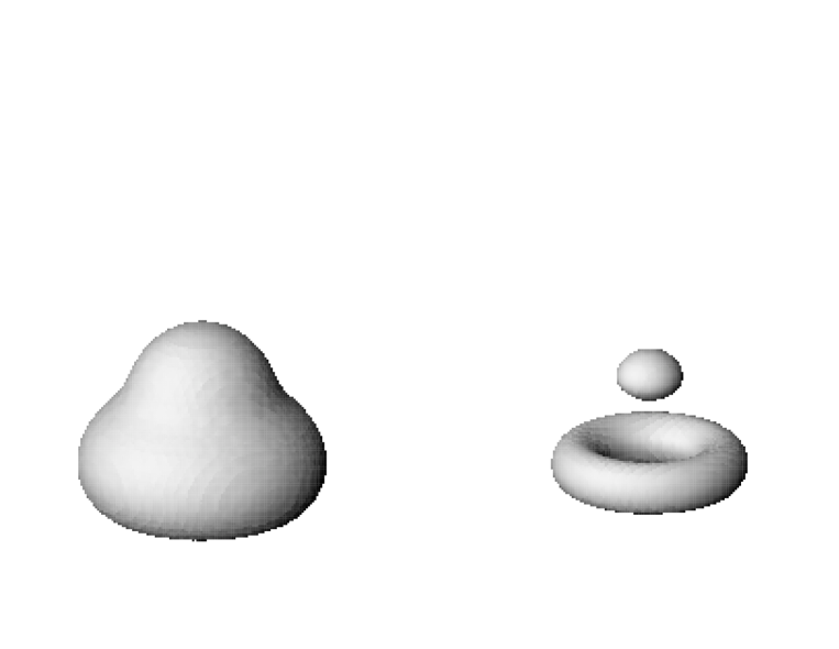
Figure 6: Baryon density for B=3: a: level=0.3 b: level=0.7

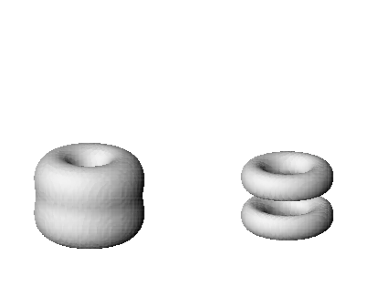
Figure 7: Baryon density for B=4: a: level=0.4 b: level=0.7

$B=4$

For $B=4$ we find

$$f=\left(\xi^{4},\,2.7191\,\xi^{2},\,1\right)^{t}.$$ (50)

This configuration also leads to the energy and baryon densities that are axially symmetric and they have the shape of two tori on top of each other. In Figures 7a and 7b, we present plots of the surfaces of the baryon densities at two values.

Once again, the densities corresponding to (50) are invariant with respect to a rotation $\xi\rightarrow\xi^{\prime}=\xi e^{i\alpha}$. Note that the baryon density for (49) does vanish when $\xi$ is zero or when its modulus $|\xi^{2}|$ is infinite. This happens since the three terms in the numerator of (47) have a single common factor at $\xi=0$, and the second term of $f$ is a polynomial of degree two – implying once again that the baryon density vanishes when $\xi=\infty$. Indeed, this can be seen in Figures 7a and 7b; clearly the density vanishes along the $z$-axis ($\theta=0$ and $\theta=\pi$). Once again, a similar configuration has been observed in the scattering of four $SU(2)$ monopoles [13] and skyrmions in an attractive channel [12].

$B=5$

The holomorphic vector for $B=5$ is given by

$$f=\left(\xi^{5}-2.7\,\xi,\,2\,\xi^{4}+1,\,9/2\,\xi^{3}\right)^{t}.$$ (51)

Note now that a transformation $\xi\rightarrow\xi^{\prime}=i\xi$ (ie a $90^{0}$ degree rotation around the $z$-axis) corresponds to a global $SU(3)$ transformation. Hence the densities are invariant under such transformations. Let us add that the $SU(2)$ embeddings have very different shapes and symmetries (in fact they are symmetric under $120^{0}$ rotations).

It is easy to check that the baryon density corresponding to the field in (51) does not have any holes. Despite this, one can see holes in Figure 8a and 8b; they correspond to regions of low, but non-zero, baryon density values.

Note that by taking $f$ in the form close to (51), ie

$$f=\left(\xi^{5}+{3C\over D}\,\xi,\,\,D\,\xi^{4}+C,\,\,E\,\xi^{3}\right)^{t},$$ (52)

all the three terms in the numerator of (47) have zeros when

$$\xi^{4}={3C\over D},$$ (53)

which gives four holes in the baryon density. So, since our field (51) is not very different from (52) our densities have minima; corresponding to the holes (53) partially filled in, by going from (52) to (51).

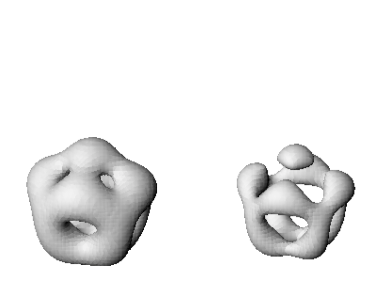
Figure 8: Baryon density for B=5: a: level=0.4 b: level=0.6

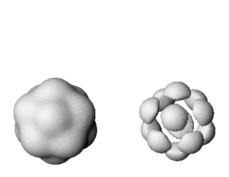
Figure 9: Baryon density for B=6: a: level=0.4 b: level=0.6

$B=6$

The holomorphic vector for $B=6$ is given by

$$f=\left(\xi^{6}+3\,\xi,\,\,1-3\,\xi^{5},\,\,k\,\xi^{3}\right)^{t},$$ (54)

where $k$ was found, numerically, to be $7.06$. Once again the baryon density of the field (54) does not have any holes but has regions where it is small but non-zero (see Figures 9a and 9b). These figures show that this configuration has an icosahedral symmetry and this leads us to the conclusion that, modulo an $SU(3)$ global transformation, (54) must be invariant under the following transformation [14]: $\xi\rightarrow\xi^{\prime}=\xi e^{{i2\pi/5}}$ (ie a rotation by $72^{0}$ around the $z$-axis); $\xi\rightarrow\xi^{\prime}=-\xi^{-1}$ (which corresponds to $\theta\rightarrow\pi-\theta$ and $\phi\rightarrow\pi-\phi$) and $\xi\rightarrow\xi^{\prime}=(\xi+b)(b\,\xi+1)^{-1}$ where $b=2\cos(2\pi/5)=(\sqrt{5}-1)/2$. This last transformation imposes a condition on $k$ in (54): it is easy to see that the $SU(3)$ transformation on $f$ must be of the form $U=R/\det(R)^{1/3}$ with

$$R=\left(\begin{array}[]{lll}\hskip 14.22636pt25+15a&\,\,10+5a&\hskip 14.22636pt(150+100)k^{-1}\\[5.69054pt] \hskip 14.22636pt10+5a&25+15a&-(150+100\,a)k^{-1}\\[5.69054pt] -k(3+2a)&k(3+2a)&\hskip 14.22636pt\,\,\,\,\,15+10a\\[5.69054pt] \end{array}\right),$$ (55)

where $a=-(1+\sqrt{5})/2$. Imposing the condition that the rows and columns of $R$ are orthogonal to each other implies that $k=\sqrt{5}0\approx 7.071$ which is within the precision of our numerical minimisation programme.

Having presented our field configurations we can now discuss some of their properties and compare them with the $SU(2)$ embeddings.

First of all, for $B=1$ we have only the $SU(2)$ embedding. Its energy and baryon density is in the shape of a ball. For $B>1$ our field configurations are different from the $SU(2)$ embeddings. However, the densities of the baryon densities for $B\leq 4$ are all axially symmetric (see Figure 5). The $B=2$ configuration is radially symmetric and the baryon density corresponds to a shell (in contrast to the toroidal $SU(2)$ one); the $B=3$ configuration corresponds to a single skyrmion located around the north pole of the $S^{2}$ sphere and the other two are below the equator (spread out to form a charge two torus-like structure), while the $B=4$ configuration consists of four baryons which are in the shape of two partially overlapping tori close to the equator of the sphere. The fields for $B>4$ are more complicated, their baryon densities have fewer symmetries as seen from our figures. The baryon and energy densities for the case of $B=5$ resemble a structure consisting of two deformed tori, close to the equator, with an additional ball at the north pole of the angular sphere while for $B=6$ they form a structure which is icosahedrally symmetric.

These shapes are very different from what was seen for $SU(2)$ fields and, as we have discussed above, they have also different symmetries.

In Figure 4, where we have plotted the energy profile functions for baryon numbers from two to six we note that the effective size of the baryons increases with the increasing baryon number – this is reflected in the shift to the right of the profile functions.

In the following table we present the energy values of the resulting Skyrme fields. All the numerical values of the energies are given in units of $B$ and hence are close to unity. These values are then compared with the $SU(2)$ skyrmion embeddings obtained using rational maps in [1]. We see that both field configurations have similar values of energy, although the energies of the embeddings are marginally lower.

$B$	${\cal I}\,(SU(3))$	$SU(3)$ En/Sk (Ansatz)	$SU(2)$ En/Sk (Ansatz)	$SU(2)$ En/Sk (Numerical)
1	1	1.232	1.232	1.232
2	4	1.222	1.208	1.171
3	10.65356	1.215	1.184	1.143
4	18.04501	1.184	1.137	1.116
5	27.26	1.164	1.147	1.116
6	37.33	1.1458	1.137	1.109

Table 2: Energy of $SU(3)$ harmonic ansatz compared to the energy of the $SU(2)$ harmonic ansatz and the energy of the $SU(2)$ solutions obtained numerically [1].

7 CONCLUSIONS

In this paper, we have discussed various static field configurations of the $SU(N)$ Skyrme model. We have shown that, in addition to the obvious embeddings, any solution of the $SU(2)$ model generates a solution of the $SU(4)$ model. Unfortunately, this solution is topologically trivial (ie its baryon density vanishes identically) and its energy is four times the original $SU(2)$ solution.

Next we have generalised the harmonic map ansatz of Houghton at al [1] and showed that this ansatz has allowed us to find another exact solution, this time of, the $SU(3)$ model. The baryon number of this solution is also zero and its energy density is radially symmetric. However, its total energy is less than four in topological units and we have argued that it represents a bound state of two skyrmions and two anti-skyrmions.

Using our generalisation of the harmonic map ansatz we have then presented topologically nontrivial field configurations of the $SU(N)$ Skyrme model with radially symmetric energy densities. They correspond to $B=N-1$ skyrmions in $SU(N)$ models. In the massless case their energies have turned out also to be above those of the $SU(2)$ embeddings. However, when mass is added to the model, for sufficiently large masses, their energies can be be lower than the energies of the embeddings.

We have also looked at various field configurations of the $SU(3)$ model. The energy and baryon densities of these $SU(3)$ fields exhibit shell-like structures; in all cases, except for $B=1$, they are different from the corresponding structures seen in the $SU(2)$ model and more symmetrical. Their energies are slightly higher but comparable to those of the embeddings. Their different symmetry properties suggest to us that although these embeddings have higher energies they may be reflections of real states of the model showing that the $SU(3)$ model can have many interesting solutions. To see whether this expectation is correct one has to perform numerical simulations - this so far has not been done.

Finally, our projector ansatz suggests that one might try to construct further ansatze involving two or more projectors. Such ansatze will then depend on more that one profile function. This topic is currently under investigation.

8 ACKNOWLEDGMENTS

The authors would like to thank V. Kopeliovich and J. Garraham for their help in finding a numerical mistake in the earlier report of this work (in the form of two papers).
We also thank C. J. Houghton for his interest ans correspondence about the symmetries of our field configurations.

References

- [1] C. J. Houghton, N. S. Manton and P. M. Sutcliffe, Nucl. Phys. B 510, 507 (1998).
- [2] T. H. R. Skyrme, Nucl. Phys. 31, 556 (1962).
- [3] E. Witten, Nucl. Phys. B 223, 422 (1983).
- [4] N. S. Manton, Phys. Lett. B 192, 177 (1987).
- [5] R. A. Battye and P. M Sutcliffe, Phys. Rev. Lett. 79, 363 (1997).
- [6] T. H. R. Skyrme, Proc. R. Soc. A 260, 127 (1961).
- [7] A. P. Balachandran, A. Barducci, F. Lizzi, V. G. J. Rodgers and A. Stern, Phys. Rev. Lett. 52, 887 (1984).
- [8] V.B. Kopeliovich, B.E. Schwesinger and B.E. Stern, JETP Lett. 62, 185-90 (1995).
- [9] W. J. Zakrzewski, Low dimensional sigma models (IOP, 1989).
- [10] A. Din and W. J. Zakrzewski, Nucl. Phys. B 174, 397 (1980).
- [11] A. D’Adda, P. Di Vecchia and M. Luscher, Nucl. Phys. B 146, 63 (1980).
- [12] R. A. Battye and P. M Sutcliffe, in preparation.
- [13] P. M. Sutcliffe, Nucl. Phys. 505, 517 (1997).
- [14] F. Klein, The Icosahedron, Dover Publications, (1956).