(In–)Consistencies in the relativistic description

of excited states in the Bethe–Salpeter equation

Steven Ahlig and Reinhard Alkofer

Institut für Theoretische Physik, Universität Tübingen,

Auf der Morgenstelle 14, 72076 Tübingen, Germany

Abstract

The Bethe–Salpeter equation provides the most widely used technique to extract bound states and resonances in a relativistic Quantum Field Theory. Nevertheless a thorough discussion how to identify its solutions with physical states is still missing. The occurrence of complex eigenvalues of the homogeneous Bethe–Salpeter equation complicates this issue further. Using a perturbative expansion in the mass difference of the constituents we demonstrate for scalar fields bound by a scalar exchange that the underlying mechanism which results in complex eigenvalues is the crossing of a normal (or abnormal) with an abnormal state. Based on an investigation of the renormalization of one–particle properties we argue that these crossings happen beyond the applicability region of the ladder Bethe–Salpeter equation. The implications for a fermion–antifermion bound state in QED are discussed, and a consistent interpretation of the bound state spectrum of QED is proposed.

Keywords:
Bethe–Salpeter equation, Dyson–Schwinger equations, QED bound states
PACS numbers: 11.10.St, 11.10.Gh, 11.15.Tk, 12.20.Ds

1 Introduction

In a relativistic Quantum Field Theory bound states and resonances are identified through the occurrence of pole or cut like singularities in the Green’s functions of the theory. Thus it is natural to study the four–point Green’s function when searching for two–particle bound states. Indeed, the corresponding equation has been proposed by Bethe and Salpeter [1] and subsequently been proven by Gell–Mann and Low [2] and Schwinger [3] as early as 1951. It can be interpreted as one of the Dyson–Schwinger [3, 4] equations of Quantum Field Theory and it is, thus, an inhomogeneous integral equation. Assuming the existence of a bound state signaled by a pole in the four–point function the homogeneous Bethe–Salpeter equation may be derived (see below). It allows to determine the bound state masses and covariant wave functions. Usually one employs the so-called ladder approximation which renders the homogeneous Bethe–Salpeter equation in the form of an eigenvalue problem. Hereby the eigenvalue is the square of the coupling constant, and the bound state mass has to be tuned such that the Bethe–Salpeter eigenvalue equals the given value of this constant. The covariant wave functions are then determined as the eigenfunctions of the system.

The only analytically solvable example of a Bethe–Salpeter equation is the one for two (massive) scalar particles bound by the ladder approximation to the exchange of a massless scalar field [5, 6, 7]. Despite its relative simplicity as compared to realistic systems this model, the Wick–Cutkosky model, displays already the advantages (e.g. full covariance) as well as the shortcomings (e.g. the existence of abnormal states) inherent to almost all Bethe–Salpeter based approaches used until today, for a recent very accurate numerical solution of the ladder Bethe–Salpeter equation for scalars see e.g. [8] and references therein.

Common to the analytical and the numerical solutions is the existence of abnormal states which have led to controversial discussions regarding their physical interpretation [5, 6, 7, 9, 10]. Even worse, for the case of constituents with unequal masses some eigenvalues of the homogeneous Bethe–Salpeter equation become complex [11, 12, 13]. Clearly, such a behavior is unexpected and has to be understood. It is usually attributed to the use of the ladder approximation which destroys crossing symmetry from the very beginning. However, we will see in the following that already the use of bare propagators is problematic. This will also not be cured by incorporating one–particle self–energies and thereby generalising the ladder approximation. Instead, it will be shown in this paper that the occurrence of complex eigenvalues also happens with self–energies taken into account. It seems that one has to start on a more fundamental level: One seriously has to raise the question which values of the renormalized coupling constant are possible when considering a renormalized Quantum Field Theory.

1.1 Derivation of the homogeneous Bethe–Salpeter equation

In order to make this paper as self–contained as possible, and to make our argumentation accessible to non–expert readers, we will supply some important derivations and facts concerning the Bethe–Salpeter approach to relativistic bound states in the remainder of this introduction. Readers familiar with the Bethe–Salpeter equation probably will probably prefer to jump to Sec. 2 immediately.

We assume to deal with three types of scalar fields. The two constituents are supposed to have masses $m_{1}$ and $m_{2}$ and self–energies $\Sigma_{1}$ and $\Sigma_{2}$. The four–point function $G^{\left(4\right)}\left(x_{1},x_{2},y_{1},y_{2}\right)$ describing the scattering of these two constituents fulfills the inhomogeneous Bethe–Salpeter equation

$$\left[\square_{x_{2}}+m_{2}^{2}-\Sigma_{2}\right]\left[\square_{x_{1}}+m_{1}^{2}-\Sigma_{1}\right]G^{\left(4\right)}\left(x_{1},x_{2},y_{1},y_{2}\right)=\quad\quad\quad\quad\quad\quad$$ (1)

$$\quad\quad\quad\quad\delta^{\left(4\right)}\left(x_{1}-y_{1}\right)\delta^{\left(4\right)}\left(x_{2}-y_{2}\right)+\delta^{\left(4\right)}\left(x_{1}-y_{2}\right)\delta^{\left(4\right)}\left(y_{1}-x_{2}\right)$$

$$\quad\quad\quad\quad\quad\quad\quad\quad\quad\quad\quad+\int d^{4}z_{1}d^{4}z_{2}K\left(x_{1},y_{1},z_{1},z_{2}\right)G^{\left(4\right)}\left(z_{1},z_{2},y_{1},y_{2}\right).$$

The kernel $K$ is defined as the sum of all amputated two–particle irreducible contributions. The Feynman diagrams of the first few terms are depicted in fig. 1.

For translationally invariant systems it is, of course, advantageous to transform this equation to momentum space. Note that the introduction of the relative coordinate $x=x_{1}-x_{2}$ allows an arbitrary parameter $\alpha\in[0,1]$ in defining the coordinate $X=\alpha x_{1}+(1-\alpha)x_{2}$ which results in the corresponding momenta

$$p_{1}=\alpha P+p\quad{\rm and}\quad p_{2}=(1-\alpha)P-p$$ (2)

for the constituents in terms of the total and relative momenta, $P$ and $p$, respectively. Fourier transforming eq. (1) leads to

$$\int\frac{d^{4}p^{\prime}}{\left(2\pi\right)^{4}}\left[{D}\left(p,p^{\prime},P\right)+{K}\left(p,p^{\prime},P\right)\right]{G}^{\left(4\right)}\left(p^{\prime},p^{\prime\prime},P\right)=\delta^{\left(4\right)}\left(p-p^{\prime\prime}\right),$$ (3)

where

$${D}\left(p,p^{\prime},P\right):=\left(2\pi\right)^{4}\delta^{\left(4\right)}\left(p-p^{\prime}\right)\left({G}_{1}^{\left(2\right)}\right)^{-1}\left(p_{1}\right)\left({G}_{2}^{\left(2\right)}\right)^{-1}\left(-p_{2}\right)$$ (4)

is defined in terms of the inverse two–point Green’s functions of the constituents.

Figure 1: Feynman diagrams of the first few terms in a perturbative expansion of the kernel $K$. Solid lines represent propagators of the constituents, dashed lines the propagator of the exchange particle.

=

Figure 2: Pictorial representation of the homogeneous Bethe–Salpeter equation in ladder approximation.

The crucial step from the inhomogeneous to the homogeneous Bethe–Salpeter equation consists in assuming a bound state reflecting itself in a pole in the four–point Green’s function for an on–shell momentum $P_{os}$, with $P_{os}^{2}=M^{2}$

$${G}^{\left(4\right)}\left(p,p^{\prime},P_{os}\right)=\frac{-i}{\left(2\pi\right)^{4}}\frac{{\chi}\left(p,P_{os}\right){\bar{\chi}}\left(p^{\prime},P_{os}\right)}{2\omega\left(P^{0}-\omega+i\epsilon\right)}+\rm{reg.\,terms},\,\omega:=\sqrt{{\bf P}^{2}+M^{2}}\,$$ (5)

where we introduced the definition of the Bethe–Salpeter amplitudes

$$\chi\left(x_{1},x_{2},P\right) := \left\langle 0\left|T\left\{\Phi\left(x_{1}\right)\Phi\left(x_{2}\right)\right\}\right|P\right\rangle$$

$$\bar{\chi}\left(x_{1},x_{2},P\right) := \left\langle 0\left|T\left\{\Phi^{\dagger}\left(x_{1}\right)\Phi^{\dagger}\left(x_{2}\right)\right\}\right|P\right\rangle$$ (6)

together with their Fourier transforms

$$\chi\left(x_{1},x_{2},P\right) =: e^{-iPX}\int\frac{d^{4}p}{\left(2\pi\right)^{4}}e^{-ipx}{\chi}\left(p,P\right)$$

$$\bar{\chi}\left(x_{1},x_{2},P\right) =: e^{+iPX}\int\frac{d^{4}p}{\left(2\pi\right)^{4}}e^{-ipx}{\bar{\chi}}\left(p,P\right).$$ (7)

Hereby $\left|0\right\rangle$ denotes the ground state (vacuum) and $\left|P\right\rangle$ the bound state. Very close to the pole the regular terms can be safely neglected and the dependence of the four–point function on the relative momenta $p$ and $p^{\prime}$ can be separated. Expanding ${G}^{\left(4\right)}$ and $\left[{D}-{K}\right]$ in the inhomogeneous Bethe–Salpeter equation in powers of $\left(P^{0}-\omega\right)$ yields the homogeneous Bethe–Salpeter equation and the normalisation condition for the amplitude. The order $\left(P^{0}-\omega\right)^{-1}$ provides

$$\int\frac{d^{4}p^{\prime}}{\left(2\pi\right)^{4}}\left[{D}\left(p,p^{\prime},P_{os}\right)+{K}\left(p,p^{\prime},P_{os}\right)\right]{\chi}\left(p,P_{os}\right)=0,$$ (8)

whereas to ${\cal O}\left(\left(P^{0}-\omega\right)^{0}\right)$ one obtains

$$\int\frac{d^{4}p}{\left(2\pi\right)^{4}}\frac{d^{4}p^{\prime}}{\left(2\pi\right)^{4}}{\rm tr}\left({\bar{\chi}}\left(p,P_{os}\right)\left.\frac{\partial}{\partial P^{0}}\left(D\left(p,p^{\prime},P\right)+K\left(p,p^{\prime},P\right)\right)\right|_{P^{0}=\omega}\!\!\!{\chi}\left(p^{\prime},P_{os}\right)\right)$$

$$=2i\omega.$$ (9)

This ensures the residue to be equal to $1$ at the bound state pole.

The homogeneous Bethe–Salpeter equation (8) is a linear integral equation for the amplitude ${\chi}$ whose overall normalisation is fixed by (9). Approximating the kernel by the one–boson–exchange depicted in the first diagram of fig. 1 eq. (8) can be cast into an eigenvalue problem for the coupling constant by defining the vertex function $\Gamma\left(p,P\right)$:

$${\chi}\left(p,P\right)=:G_{1}\left(p_{1}\right)G_{2}\left(p_{2}\right)\Gamma\left(p,P\right).$$ (10)

The homogeneous Bethe–Salpeter equation (8) then reads

$$\Gamma\left(p,P_{os}\right)=-\int\frac{d^{4}p^{\prime}}{\left(2\pi\right)^{4}}K\left(p,p^{\prime},P_{os}\right)G_{1}\left(p_{1}^{\prime}\right)G_{2}\left(p_{2}^{\prime}\right)\Gamma\left(p^{\prime},P_{os}\right).$$ (11)

In the ladder approximation the kernel $K$ is set equal to

$$K(p,p^{\prime})=i\frac{g^{2}}{(p-p^{\prime})^{2}-\mu^{2}}$$ (12)

which is just the propagator of the scalar exchange particle of mass $\mu$ multiplied with $g^{2}$. On inspection one finds that (11) is an eigenvalue problem for $g^{2}$ if $G_{1}$ and $G_{2}$ are the bare propagators of the constituents. The ladder approximation to the Bethe-Salpeter equation is pictorially represented in fig. 2. If a parameter pair $(g^{2},P^{0}=M)$ exists the pole assumption is a posteriori justified and $M$ is the bound state mass with $\chi$ being the corresponding amplitude (wave function) as can be inferred from eq. (5) which reflects, of course, nothing else than the Lehmann representation of the four–point function.

1.2 Abnormal solutions and relative time parity

For a given bound state mass $M$ the eigenvalue spectrum of the Bethe–Salpeter equation should be positive definite, i.e. the eigenvalues should be real and positive. We will see that this is not the case. Furthermore, one expects that for very small coupling constants the binding energy vanishes and the bound state mass becomes identical to the sum of the masses of the constituents. There are states, however, which possess vanishing binding energy for a finite coupling. They are therefore called abnormal states. In the Wick–Cutksoky model [5, 6] with constituents of equal masses $m_{1}=m_{2}=m$ these abnormal states are easily identified: They only exist for $\lambda:=g^{2}/16\pi^{2}m^{2}>\lambda_{c}=1/4$. If the binding energy becomes very small, i.e. $\eta:=M/2m\to 1$, the corresponding coupling constant $\lambda$ vanishes for the normal solutions, i.e. $\lambda\to 0$, whereas $\lambda\to\lambda_{c}=1/4$ for the abnormal states, see fig. 3 and its closeup fig. 4.

Figure 3: The eigenvalues of the Bethe–Salpeter equation in the Wick–Cutksoky model with constituents of equal masses as a function of the ratio of bound state mass to the sum of masses of the constituents,$\eta=M/2m$ .

Figure 4: Same as fig. 3, however, for $\eta$ close to one.

On the other hand, in the opposite limit of a massless bound state, i.e. for $\eta\to 0$, the eigenvalues are given by [6]

$$\lambda=\left(n+\kappa\right)\left(n+\kappa+1\right)=N\left(N+1\right).$$ (13)

The value of $\kappa$ equals the number of nodes of the eigenfunctions when plotted as a function of the relative time $x_{0}$. For all normal solutions, including the ground state, one has $\kappa=0$. This especially means that all normal solutions are even under the reversal of relative time $x_{0}\rightarrow-x_{0}$. On the other hand, $\kappa=1,2,\ldots$ leads to abnormal solutions, i.e. these solutions may be even or odd with respect $x_{0}\rightarrow-x_{0}$:

$$\chi\left(-x_{0},\mathbf{x}\right)=\left(-1\right)^{\kappa}\chi\left(x_{0},\mathbf{x}\right).$$ (14)

One may interpret the abnormal solutions as excitations in relative time. They will obviously not appear in a purely non–relativistic treatment where the constituents are considered for equal times only. However, not all abnormal solutions necessarily vanish in a three–dimensional reduction of the Bethe–Salpeter equation [14]. On the contrary, the spectrum of a three–dimensionally reduced equation will contain remnants of these abnormal states.

Figure 5: The lowest lying three eigenvalues of the ladder Bethe–Salpeter equation for $\delta=m_{1}/m_{2}=4$ and $\mu=m_{2}$.

For constituents of unequal masses and a massless exchange particle the Bethe–Salpeter amplitudes are asymmetric, i.e. neither even nor odd, under the transformation $x_{0}\rightarrow-x_{0}$. However, the eigenvalues of the abnormal states start all at some common $\lambda_{c}$, see also [7] and references therein.

For equally massive constituents and a massive exchange particle the amplitudes do have a definite “parity” under the inversion of relative time. However, there is no longer a common $\lambda_{c}$ at which the eigenvalues of the abnormal solutions start.

The controversial discussion of the abnormal states already started with the work of Wick [5] and Cutkosky [6], for some of the related investigations see also [9, 15, 7]. Fixing the spatial coordinates of the constituents leaving only the relative time as degree of freedom one is able to show that the abnormal solutions are all unphysical for this “static” model [10]. However, it is not clear whether abnormal solutions can in general be considered as unphysical [16]. As already mentioned, some of these abnormal solutions survive most three–dimensional reductions [14]. Based on the analysis of several reductions of the Bethe–Salpeter equation the main conclusion of ref. [14] is that abnormal solutions are very probably spurious consequences of the ladder approximation supporting hereby an old conjecture by Wick [5].

$~{}~{}~{}~{}~{}~{}~{}~{}~{}~{}~{}~{}~{}~{}M,\mu~{}~{}~{}~{}~{}~{}~{}~{}~{}~{}~{}~{}~{}~{}$	symmetry group	Bethe–Salpeter amplitude
$M=0,\mu=0$	$O\left(5\right)$	$\chi\propto Z_{nklm}\left(\Omega_{5}\right)$
$M=0,\mu\neq 0$	$O\left(4\right)$	$\chi\propto Z_{klm}\left(\Omega_{4}\right)$
$M\neq 0,\mu=0$	$O\left(4\right)$	$\chi\propto Z_{klm}\left(\Omega_{4}\right)$
$M\neq 0,\mu\neq 0$	$O\left(3\right)$	$\chi\propto Y_{lm}\left(\Omega_{3}\right)$
$\mu\rightarrow\infty$	$O\left(4\right)$	$\chi\propto Z_{klm}\left(\Omega_{4}\right)$

Table 1: Summary of the symmetries of the scalar Bethe–Salpeter equation in ladder approximation. $\mu$ denotes the mass of the exchange particle and $M$ is the Mass of the bound state. The functions $Z$ (or $Y$) denote the spherical harmonics for the corresponding $n$-sphere $\Omega_{n}$.

1.3 Complex eigenvalues

In this subsection we will consider the general case for a Bethe-Salpeter equation containing only scalars: the masses of the constituents are assumed to be unequal, the exchange particle is chosen to be massive. The numerical method is detailed in appendix A and we will only give results here. For comparable sets of parameters our results are equal to those given in refs. [12, 13]. In fig. 5 the lowest three eigenvalues for $\delta=m_{1}/m_{2}=4$ and $\mu=m_{2}$ are shown as a function of $\eta=M/(m_{1}+m_{2})$. The eigenvalue of the ground state is real for all physically allowed values $\eta\in[0,1]$ and vanishes for $\eta\to 1$. The ground state is thus a normal state. The situation differs drastically for the higher–lying two states. At $\eta=1$ the eigenvalues are non–vanishing, real and positive. As the binding energy increases these two levels become degenerate at $\eta\approx 0.81$. In the interval given approximately by $0.25<\eta<0.81$ the eigenvalues are complex with a degenerate real part and imaginary parts of opposite sign. As one can see in fig. 5 from the projection of the curves not all eigenvalues are monotonically decreasing as a function of $\eta$. Clearly, such a behaviour is unphysical because a decreasing coupling constant should result in less binding.

The appearance of complex eigenvalues is not restricted to a special choice of parameters. In fig. 6 the absolute value of the imaginary part of the eigenvalues for the first two excited states is shown for $\mu=m_{2}$ and $1<\delta\leq 15$. One clearly sees that with the increase in the mass of one constituent the interval in $\eta$ for which the eigenvalues are non–real becomes smaller, however, the maximum value of the imaginary part even increases. For a given mass ratio $\delta$ complex eigenvalues exist for masses of the exchange particle up to some $\mu_{\rm max}$, i.e. for $0<\mu\leq\mu_{\rm max}$. Considering the first two excited states we estimate this $\mu_{\rm max}$ to be $\mu_{\rm max}\approx 0.85m_{1}+1.66m_{2}$. Increasing the mass of the exchange particle the higher lying eigenvalues tend to become real again. This can be understood from the fact that for an infinitely heavy exchange particle the Bethe–Salpeter equation assumes an $O(4)$ symmetric form as in the case of an massless exchange particle, see also table 1 which summarises the symmetries of the scalar ladder Bethe–Salpeter equation.

Figure 6: The absolute value of the imaginary part of the eigenvalues for the first two excited states.

2 Inconsistency of the abnormal states

In this section we relate the appearance of complex eigenvalues of the Bethe–Salpeter– (BS) equation to the presence of the abnormal solutions. To this end we verify a conjecture of Kaufmann [11].

In section 1.1 we recalled the steps leading from the inhomogeneous BS equation (1) to the homogeneous BS equation (8). We now Wick-rotate the contour of integration in (8) according to $p_{0}\rightarrow ip_{4},\mathbf{p}\rightarrow\mathbf{p}$ and thus obtain the homogeneous BS equation for euclidean momenta. A subsequent Fourier–transformation yields the homogeneous BS equation in euclidean coordinate–space:

$${\cal L}\chi=\left[{\cal L}_{0}+{\cal P}\right]\chi=\bar{\lambda}{\cal V}\chi.$$ (15)

The operator ${\cal L}$ is the product of the inverse propagators of the constituents and $\chi$ is the BS amplitude describing a bound state of two scalar particles with masses $m_{1}$ and $m_{2}$, respectively. The interaction of the two constituents is encoded in ${\cal V}$ which in the ladder–approximation is simply the Fourier–transform of the bare propagator of the exchange–particle. We decomposed the operator ${\cal L}$ into two parts: ${\cal L}_{0}$, containing the terms that are present for $m_{1}=m_{2}$ and ${\cal P}$ containing the additional terms that appear only for $m_{1}\neq m_{2}$. The eigenvalue is denoted by $\bar{\lambda}$ instead of $\lambda$ for later convenience. The explicit expressions are given by:

$${\cal L}_{0} = \left[\tilde{p}^{2}+2\eta\left(i\tilde{p}_{4}\right)+1-\eta^{2}\right]\left[\tilde{p}^{2}-2\eta\left(i\tilde{p}_{4}\right)+1-\eta^{2}\right]\quad\quad$$

$${\rm with} \quad\tilde{p}_{\mu}=i\partial_{\mu}/m_{2}$$

$${\cal P} = \left(i\tilde{p}_{4}\right)\left[4\eta\Delta\left[\tilde{p}^{2}-\left(1-\eta^{2}\right)\right]+\Delta^{3}4\eta\left(1-\eta^{2}\right)\right]$$ (17)

$$+ \Delta^{2}\left[2\left(1-\eta^{2}\right)\left[\tilde{p}^{2}-\left(1-\eta^{2}\right)\right]-4\eta^{2}\tilde{p}_{4}^{2}\right]+\Delta^{4}\left(1-\eta^{2}\right)^{2}$$

$${\cal V} = \frac{1}{\pi^{2}}\int d^{4}q\frac{e^{-iq\cdot x}}{q^{2}+\mu^{2}}$$ (18)

$$\bar{\lambda} = \frac{g^{2}}{16\pi^{2}m_{2}^{2}}$$ (19)

The parameter $\eta=M/(m_{1}+m_{2})$ measures the mass of the bound state, $\Delta=(m_{1}-m_{2})/2m_{2}$ is proportional to the mass difference, and $\mu$ is the mass of the exchange–particle.

The explicit expression (17) shows that ${\cal P}$ vanishes for a vanishing mass difference $\Delta$. Thus for small $\Delta$ the decomposition ${\cal L}={\cal L}_{0}+{\cal P}$ can be understood as dividing ${\cal L}$ into the dominant part ${\cal L}_{0}$ and into the perturbation ${\cal P}$. In the following we will formalise this point of view and investigate the consequences thereof.

Suppose $\chi_{1}$ and $\chi_{2}$ are two solutions of the homogeneous BS equation for constituents of equal mass with eigenvalues $\lambda_{1}$ and $\lambda_{2}$ respectively:

$${\cal L}_{0}\chi_{1} =\lambda_{1}{\cal V}\chi_{1}$$

$${\cal L}_{0}\chi_{2} =\lambda_{2}{\cal V}\chi_{2}$$ (20)

Because of the restriction $m_{1}=m_{2}$ the BS amplitudes $\chi_{1}$ and $\chi_{2}$ have a definite $x_{0}$-parity. As we will see the interesting case is to take $\chi_{1}$ and $\chi_{2}$ to be of opposite $x_{0}$–parity, and this is assumed for the following considerations. Since we are interested in the region where two real solutions become a pair of complex conjugated solutions we take the ansatz $\chi=a\chi_{1}+b\chi_{2}$ where $\chi$ is the BS amplitude for different masses $m_{1}\neq m_{2}$ and $\chi_{1},\chi_{2}$ are the amplitudes for $m_{1}=m_{2}$ as defined in (20). Substituting this ansatz for $\chi$ into (15) and projecting onto $\chi_{1}$ and $\chi_{2}$ one obtains a system of equations relating the eigenvalue $\bar{\lambda}$ to the eigenvalues $\lambda_{1},\lambda_{2}$:

$$a\lambda_{1}{\cal V}_{11}+a{\cal P}_{11}+b{\cal P}_{12} =\bar{\lambda}a{\cal V}_{11}$$

$$b\lambda_{2}{\cal V}_{22}+a{\cal P}_{21}+b{\cal P}_{22} =\bar{\lambda}b{\cal V}_{22}$$ (21)

where

$$X_{ik}=\langle\chi_{i},X\chi_{k}\rangle:=\int d^{4}x\,\chi_{i}^{*}\left(x\right)X\chi_{k}\left(x\right)$$ (22)

for $X={\cal P},{\cal V}$ and $i,k=1,2$. In deriving (21) we used ${\cal V}_{12}={\cal V}_{21}=0$ which is due to the different $x_{0}$–parity of $\chi_{1}$ and $\chi_{2}$.

Assuming $\chi_{1}$ and $\chi_{2}$ to be normalised according to ${\cal V}_{11}={\cal V}_{22}=1$ one finds the two eigenvalues $\bar{\lambda}_{1,2}$ of the BS equation (15),

$$\bar{\lambda}_{1,2}=\frac{1}{2}\left(\lambda_{1}+\lambda_{2}+{\cal P}_{11}+{\cal P}_{22}\right)\pm\sqrt{\frac{1}{4}\left(\lambda_{1}-\lambda_{2}+{\cal P}_{11}-{\cal P}_{22}\right)^{2}+{\cal P}_{12}{\cal P}_{21}}\,\,.$$ (23)

Figure 7: The real part of two colliding solutions, according to the numerical solution (solid line) and its semi–analytic estimate (23) (dashed line), c.f. also the upper left corner in fig. 5.

This gives $\bar{\lambda}$, i.e. the eigenvalue for $\Delta\neq 0$, in terms of the matrix-elements ${\cal P}_{ik}$ and $\lambda_{1},\lambda_{2}$ which are the eigenvalues for $\Delta=0$. Using the explicit expression (17) one may calculate the matrix elements ${\cal P}_{ik}$ thereby employing the solutions $\chi_{1}$ and $\chi_{2}$ obtained by numerically solving the BS equation for $\Delta=0$. On inspection one finds that ${\cal P}$ is antihermitian leading to ${\cal P}_{12}=-{\cal P}_{21}^{*}\Rightarrow{\cal P}_{12}{\cal P}_{21}=-\left|{\cal P}_{12}\right|^{2}$. According to (23) this is a necessary condition for the appearance of complex eigenvalues. This is in contrast to the hermitian perturbations that are considered usually. Whereas a hermitian perturbation will enforce a repulsion between the solutions (avoided crossing) an antihermitian perturbation will result in an attraction.

The real part of $\bar{\lambda}_{1,2}$ as calculated according to (23) together with the result of the numerical calculation is shown in fig. 7. The dashed line represents the results according to the coupling mechanism that has been proposed in this section whereas the solid line represents the results of the numerical solution of the BS equation with $\delta=m_{1}/m_{2}=4$ and $\mu=m_{2}$, c.f. the upper left corner in fig. 5. The two curves are in reasonable quantitative agreement. The simple ansatz $\chi=a\chi_{1}+b\chi_{2}$ and the coupling due to ${\cal P}$ reproduce the overall appearance of the collision astonishingly well. The imaginary parts of the solutions $\bar{\lambda}(\eta)$ appear after the collision point. They agree with those of the numerical solution to the same level as the real parts. Therefore we conclude: the coupling of solutions of opposite $x_{0}$-parity is the mechanism leading to complex eigenvalues. Hereby, the presence of solutions of positive and negative $x_{0}$-parity is a prerequisite for the appearance of complex eigenvalues $\bar{\lambda}$. Choosing both states to be of the same $x_{0}$–parity will lead to an avoided crossing. Thus, at least one abnormal state is necessary for the occurence of a pair of complex eigenvalues.

In this context it is interesting to note that Naito and Nakanishi [17] derived a normalization condition which they claimed to remove the solutions with complex eigenvalues. However, a substantial loophole has been spotted in their derivation [18] and Fukui and Setô [13] showed numerically that the normalization condition can be satisfied for solutions with real as well as for solutions with complex eigenvalues.

In the following we will show that the solutions with negative $x_{0}$-parity lead to inconsistencies on a even more fundamental level. We will derive an equation that has to be satisfied by all solutions of the BS equation in ladder approximation which, however, is only satisfied by the solutions with positive $x_{0}$–parity, see also refs. [19, 20].

The equation may be derived starting with the inhomogeneous BS equation

$$\bar{D}\left(p,P\right)G\left(p,q,P\right)=\delta^{4}\left(p-q\right)+\int d^{4}p^{{}^{\prime}}\,K\left(p,p^{\prime},P\right)G\left(p^{\prime},q,P\right)$$ (24)

where $\bar{D}$ is the product of inverse propagators

$$\bar{D}\left(p,P\right):=G_{0}^{-1}\left(p_{1}\right)G_{0}^{-1}\left(p_{2}\right),\quad p_{1}:=\alpha P+p,\quad p_{2}:=(1-\alpha)P-p,$$ (25)

and is slightly different from $D$ defined in (4). The following considerations are restricted to the case $m_{1}=m_{2}$ which is reflected in the definition (25). $G$ is the 4-point function. It depends on the total 4-momentum $P$ and the relative 4-momenta $p$ and $q$. The kernel $K$ is defined as the sum over all 2–particle irreducible diagrams. Taking the derivative with respect to $\lambda=g^{2}/16\pi^{2}m_{2}^{2}$ one obtains after some reordering

$$\int d^{4}p\,d^{4}p^{\prime}\,G\left(p^{\prime\prime},p,P\right)\left[\frac{\partial}{\partial\lambda}\bar{D}\left(p,P\right)\delta^{4}\left(p^{\prime}-p\right)-\frac{\partial}{\partial\lambda}K\left(p,p^{\prime},P\right)\right]G\left(p^{\prime},q,P\right)$$

$$=-\frac{\partial}{\partial\lambda}G\left(p^{\prime\prime},q,P\right)\,.\quad$$ (26)

No approximation has been used so far. To proceed we restrict the considerations to the case of bare propagators and to the use of the ladder approximation for the kernel $K$. This yields

$$\frac{\partial}{\partial\lambda}\bar{D}\left(p,P\right) = 0,$$

$$\frac{\partial}{\partial\lambda}K\left(p,p^{\prime},P\right) = \frac{1}{\lambda}K\left(p,p^{\prime},P\right).$$ (27)

Substituting the representation of the 4-point function as given in eq. (5) and comparing the pole contributions one obtains

$$i\int d^{4}p\,d^{4}p^{\prime}\,\overline{\chi}\left(p\right)K\left(p,p^{\prime},P\right)\chi\left(p^{\prime}\right)=\lambda\frac{dM^{2}}{d\lambda}$$ (28)

where $\chi$ is the BS amplitude. Equation (28) should be satisfied by all solutions $\chi$ of the BS equation if bare propagators and the ladder approximation for the kernel $K$ are used.

One can make use of translation invariance to factor out the center of mass motion:

$$\chi={\rm e}^{-iP\cdot X}\phi\left(x,P\right).$$ (29)

The coordinates are hereby defined according to

$$x:=x_{1}-x_{2},\quad X:=\alpha x_{1}+(1-\alpha)x_{2}$$ (30)

and the $x_{0}$–parity is reflected in the relation $\phi\left(-x^{0},\mathbf{x}\right)=\epsilon\left(\phi\right)\,\phi\left(x^{0},\mathbf{x}\right)$ with $\epsilon\left(\phi\right)=\pm 1$. In the next step one decomposes the amplitudes $\phi$ into positive and negative frequency parts, see [5]. After Wick rotation,

$$p:=(p_{0},{\bf p})\rightarrow(ip_{4},{\bf p})=:\bar{p},\qquad(\bar{p}^{2}>0),$$ (31)

one obtains the relation, see appendix B for its derivation,

$$\bar{\phi}(\bar{p},P)=\epsilon(\phi)\left[\phi(\bar{p},P)\right]^{*}$$ (32)

for the Euclidean amplitudes. Applying the Wick rotation (31) to (28) and substituting the relation (32) one arrives at

$$-\epsilon\left(\phi\right)\int d^{4}\bar{p}\,d^{4}\bar{p}^{\prime}\,\left[\phi\left(\bar{p},P\right)\right]^{*}K^{\prime}\left(\bar{p},\bar{p}^{\prime},P\right)\phi\left(\bar{p}^{\prime},P\right)=\lambda\frac{dM^{2}}{d\lambda}$$ (33)

with positive $K^{\prime}\left(\bar{p},\bar{p}^{\prime},P\right)=\left(\bar{p}-\bar{p}^{\prime}\right)^{-2}$. As was discussed in the introduction a decreasing coupling constant should result in less binding, i.e. $dM^{2}/d\lambda$ should be negative. Eq. (33) implies that this is the case only for $\epsilon\left(\phi\right)=+1$, i.e. only the states with a positive $x_{0}$–parity can satisfy both, eq.  (33) and the physical condidtion $dM^{2}/d\lambda<0$.

On the one hand, we have obtained eq. (28) that has been derived from the exact BS equation using bare propagators and the ladder approximation for the kernel. On the other hand, we found that the solutions of negative $x_{0}$–parity (being solutions of the BS equation in the same approximation) cannot satisfy this equation and behave simultaneously reasonable under the change of the coupling constant. As a matter of fact, we found in our numerical results examples for both types of behaviour, i.e. either a violation of eq. (33) or a positive slope when ploting $M^{2}$ vs.  $\lambda$. As a subset of the abnormal solutions the solutions of negative $x_{0}$–parity are present only above a certain nonzero coupling-constant. To reconcile these conflicting results one has to question the combined use of free propagators and the ladder approximation for coupling constants that are above this critical value.

3 Renormalization of one–particle properties

In this section we first present a consistent approximation scheme for the propagators and the kernel of the BS equation. The resulting system of Dyson–Schwinger equations is solved yielding a domain of validity for the ladder approximation. The equations are derived using the formalism of Cornwall, Jackiw and Tomboulis (CJT) [21].

The starting point is the generating functional

$$Z[J,K]:=\int\prod_{i}{\cal D}\Phi_{i}\exp\left(i\left[S[\Phi]+\Phi\cdot J+\frac{1}{2}\Phi\cdot K\cdot\Phi\right]\right)$$ (34)

where $\Phi_{i}(x)$ are scalar fields, $S[\Phi]$ is the classical action and the abbreviations are defined by

$$\Phi\cdot J := \sum_{i}\int d^{4}x\,\Phi_{i}\left(x\right)J^{i}\left(x\right),$$

$$\Phi\cdot K\cdot\Phi := \sum_{i,k}\int d^{4}x\,d^{4}y\,\Phi_{i}\left(x\right)K^{ik}\left(x,y\right)\Phi_{k}\left(y\right).$$ (35)

The generating functional for connected Greens functions is defined as usual by $Z\left[J,K\right]=:\exp\left(iW\left[J,K\right]\right)$. Using

$$\frac{\delta W\left[J,K\right]}{\delta J^{i}\left(x\right)} =: \phi_{i}\left(x\right)$$

$$\frac{\delta W\left[J,K\right]}{\delta K^{ik}\left(x,y\right)} =: \frac{1}{2}\left(\phi_{i}\left(x\right)\phi_{k}\left(y\right)+G_{ik}\left(x,y\right)\right)$$ (36)

and performing a double Legendre transformation one obtains the effective action $\Gamma$ as a functional of $\phi$ and $G$,

$$\Gamma\left[\phi,G\right]:=W\left[J,K\right]-\phi\cdot J-\frac{1}{2}\phi\cdot K\cdot\phi-\frac{1}{2}G\cdot K.$$ (37)

Here the notation defined in (35) has been used. In ref. [21] the expression

$$\Gamma\left[\phi,G\right]=S\left[\phi\right]+\frac{1}{2}i{\rm Tr\,Ln}\left(G^{-1}\right)+\frac{1}{2}i{\rm Tr}\left({\cal D}^{-1}G\right)+\Gamma_{2}\left[\phi,G\right]$$ (38)

has been derived where ${\cal D}^{-1}$ is given by

$$i{\cal D}_{ik}^{-1}\left(x,y;\phi\right):=iD_{i}^{-1}\left(x-y\right)\delta_{ik}+\frac{\delta^{2}S_{int}\left[\phi\right]}{\delta\phi_{i}\left(x\right)\delta\phi_{k}\left(y\right)},$$ (39)

and $D$ is the bare propagator. The nontrivial part in the effective action (38) is $\Gamma_{2}$. It is defined as a sum of vacuum loops where the vertices are given by the interaction part of $S[\Phi+\phi]$ and the propagators are equal to $G_{ik}$.

The BS equation for the amplitude $\psi$ in its most general form is given by

$$\int d^{4}x^{\prime}\,d^{4}y^{\prime}\,\Gamma_{ik,i^{\prime}k^{\prime}}^{\left(2\right)}\left(x,y;x^{\prime},y^{\prime}\right)\psi^{i^{\prime}k^{\prime}}\left(x^{\prime},y^{\prime}\right)=0$$ (40)

where $\Gamma_{ik,i^{\prime}k^{\prime}}^{\left(2\right)}\left(x,y;x^{\prime},y^{\prime}\right)$ is the 2nd functional derivative of $\Gamma$ with respect to $G$. The propagators $G$ are the solution of the corresponding Dyson-Schwinger equations

$$\frac{\delta\Gamma\left[\phi,G\right]}{\delta G_{ab}\left(x,y\right)}=0.$$ (41)

In the following we will consider a theory of three scalar fields $\Phi_{1},\Phi_{2}$ and $\Phi_{3}$ describing massive particles and interacting according to the Lagrangian

$${\cal L}=\sum_{i}\frac{1}{2}\partial_{\mu}\Phi_{i}\partial^{\mu}\Phi_{i}-\sum_{i}\frac{1}{2}m_{i}^{2}\Phi_{i}^{2}+\frac{g}{\sqrt{2}}\left(\Phi_{1}^{2}+\Phi_{2}^{2}\right)\Phi_{3}.$$ (42)

We approximate $\Gamma_{2}$ by the first nontrivial term of the loop-expansion, i.e. we use

$$\Gamma_{2} =$$

$$= \frac{1}{4}g^{2}\int d^{4}x^{\prime}\,d^{4}y^{\prime}\,\left(\sum_{i,k=1}^{2}G_{ik}^{2}(x^{\prime},y^{\prime})G_{33}(x^{\prime},y^{\prime})\right.$$

$$\quad\quad\quad\quad\quad\quad\,\,\,\,\,\left.+\sum_{i=1}^{2}G_{ii}^{2}(x^{\prime},y^{\prime})G_{33}(x^{\prime},y^{\prime})\right)\,.$$

This approximation for $\Gamma_{2}$ results in the rainbow–ladder approximation for the BS equation (40) and the Dyson–Schwinger equations (41). Having evaluated the functional derivatives we Fourier transform the resulting system of equations to momentum–space thus obtaining the BS equation

$$G_{1}^{-1}\left(p_{1}\right)G_{2}^{-1}\left(p_{2}\right)\psi^{12}\left(p,P\right)=g^{2}i\int\frac{d^{4}q}{\left(2\pi\right)^{4}}\,G_{3}\left(p-q\right)\psi^{12}\left(q,P\right)$$ (44)

for the BS amplitude $\psi^{12}$ describing a bound states of particles 1 and 2. The momenta are defined by

$$p_{1}:=p-\alpha P,\quad p_{2}:=p+\left(1-\alpha\right)P.$$ (45)

Evaluating explicitely the functional derivative (41) we obtain the coupled system of Dyson-Schwinger equations:

$$G_{i}^{-1}\left(p\right) = D_{i}^{-1}\left(p\right)-2g^{2}i\int\frac{d^{4}q}{\left(2\pi\right)^{4}}\,G_{3}\left(p-q\right)G_{i}\left(q\right)\quad\quad i=1,2$$ (46)

$$G_{3}^{-1}\left(p\right) = D_{3}^{-1}\left(p\right)-g^{2}i\int\frac{d^{4}q}{\left(2\pi\right)^{4}}\,\sum_{i=1,2}G_{i}\left(p-q\right)G_{i}\left(q\right)$$ (47)

for the propagators $G_{i}$ that are used in the BS equation. This system of equations is depicted diagrammatically in fig. (8).

$\biggl{(}\begin{minipage}{56.9055pt} \psfig{width=56.9055pt} \end{minipage}\biggr{)}^{-1}=\hskip 11.38109pt\biggl{(}\begin{minipage}{56.9055pt} \psfig{width=56.9055pt} \end{minipage}\biggr{)}^{-1}+\hskip 11.38109pt\begin{minipage}{56.9055pt} \psfig{width=56.9055pt} \end{minipage}$

$\biggl{(}\begin{minipage}{56.9055pt} \psfig{width=56.9055pt} \end{minipage}\biggr{)}^{-1}=\hskip 11.38109pt\biggl{(}\begin{minipage}{56.9055pt} \psfig{width=56.9055pt} \end{minipage}\biggr{)}^{-1}+\hskip 11.38109pt\begin{minipage}{56.9055pt} \hskip 5.69046pt \psfig{width=39.83368pt} \end{minipage}$

Figure 8: Graphical representation of the coupled system of Dyson-Schwinger equations (46), (47). Thick and thin lines represent the dressed and the bare propagators, respectively.

Up to now we have used the unrenormalized fields $\Phi_{i}$, masses $m_{i}$ and coupling constant $g$. Introducing the corresponding renormalized quantities $\bar{\Phi}_{i},\bar{m}_{i},\bar{g}$ through

$$\sqrt{Z_{i}}\bar{\Phi}_{i}=\Phi_{i},\quad Z_{m_{i}}\bar{m}_{i}^{2}=m_{i}^{2},\quad Z_{g}\bar{g}=g$$ (48)

one is able to repeat the steps leading from (41) to (46) and (47). As we use bare vertices (rainbow approximation) we have to set $Z_{g}=1$ for consistency. This procedure yields the Dyson-Schwinger equations for the renormalized self-energies $\Sigma(p^{2}):=p^{2}-m^{2}-G^{-1}(p)$

$$\Sigma_{i}\left(p^{2}\right) = \Delta_{i}+Z_{i}2g^{2}i\int\frac{d^{4}q}{\left(2\pi\right)^{4}}\,G_{3}\left(p-q\right)G_{i}\left(q\right)\quad\quad i=1,2$$ (49)

$$\Sigma_{3}\left(p^{2}\right) = \Delta_{3}+g^{2}i\int\frac{d^{4}q}{\left(2\pi\right)^{4}}\,\sum_{i=1,2}Z_{i}G_{i}\left(p-q\right)G_{i}\left(q\right)$$ (50)

where the abbreviation

$$\Delta_{i}:=\left(1-Z_{i}\right)p^{2}+\left(Z_{i}Z_{m_{i}}-1\right)m_{i}^{2}\qquad i=1,2,3$$ (51)

has been used. This coupled system of Dyson–Schwinger equations is finally defined by fixing the renormalization constants according to the on–shell renormalization

$$\Sigma_{i}\left(m_{i}^{2}\right)=\left.\frac{d}{dp^{2}}\Sigma_{i}\left(p^{2}\right)\right|_{p^{2}=m_{i}^{2}}=0.$$ (52)

Note that the Lagrangian (42) defines a super–renormalizable model. Thus, the mass renormalization constants $Z_{m_{i}}$ are logarithmically instead of quadratically divergent, the field renormalization constants $Z_{i}$ are finite. We take them nevertheless into account in order to mimic an exactly renormalizable theory as closely as possible.

In order to obtain a numerical solution a Wick rotation to Euclidean space is performed. The resulting coupled system of integral equations is then solved iteratively. The details of the numerical method are given in appendix C.

Since we are interested in the domain of validity of the ladder approximation we focus on the physical constraints to be satisfied by the propagators. The quanta of the fields $\Phi$ are assumed to describe physical particles. This implies that the associated renormalization constants $Z_{i}$ and $Z_{m_{i}}$ are positive and smaller than 1, i.e. $0\leq Z_{i},Z_{m_{i}}\leq 1$.

Figure 9: The dependence of the renormalization constants $Z_{2}(\mu=m_{2})$ and $Z_{m_{2}}(\Lambda_{UV},\mu=m_{2})$ on $\lambda=g^{2}/16\pi^{2}m_{2}^{2}$. The renormalized masses of the constituents were taken to be $m_{1}/m_{2}=4$ and the mass of the exchange particle was set equal to $m_{2}$.

The dependence of the renormalization constants $Z_{i}$ and $Z_{m_{i}}$ on the coupling parameter $\lambda=g^{2}/16\pi^{2}m_{2}^{2}$ displays an interesting behaviour. Fig. 9 shows the results for $Z_{2}$ and $Z_{m_{2}}$ which are the renormalization constants for the less massive field $\Phi_{2}$. The masses of the constituents were taken to be $m_{1}/m_{2}=4$ and the mass of the exchange particle was set equal to $m_{2}$. $Z_{2}$ and $Z_{m_{2}}$ start at one for small values of the coupling constant and decrease for greater values. Both, the mass renormalization $Z_{m_{2}}$ as well as the field renormalization $Z_{2}$ become negative at some critical value of the coupling constant. These critical values are $\lambda\approx 0.062$ corresponding to $g/m_{2}\approx 3.13$ for $Z_{m_{2}}$ and $\lambda\approx 0.086$ corresponding to $g/m_{2}\approx 3.68$ for $Z_{2}$. Since the propagator for particle 2 enters the BS equation we conclude that the domain of validity of the system of equations (44), (46), (47) is limited to the range $0\leq g/m_{2}\leq 3.13$. A negative value for $Z_{m_{2}}$ especially implies that $m_{2}^{2}<0$, i.e. particle 2 becomes tachyonic. Note also that in ref. [22] the critical value $\lambda_{c}\approx 0.063$ of the coupling constant was found using a variational approach.

It remains to solve the BS equation thereby employing the dressed propagators which are the solution of (49) and (50). Restricting the calculations to the allowed range of the coupling constant $g$ one does find that the inclusion of the self-energies somewhat lowers the solutions $g(M)$, however, the deviations are much smaller than $1\%$. Leaving the domain of validity i.e. going beyond $g/m_{2}\approx 3.68$ one does find a growing influence of the self-energies as could be expected. For $g/m_{2}\gg 3.68$ we also found complex eigenvalues $\lambda$.

The effect of the inclusion of the set of crossed ladders has been investigated by Nieuwenhuis and Tjon [23]. They used the Feynman-Schwinger representation which takes account of the ordinary as well as the crossed ladders. Within this framework they calculated the binding energy of the ground state and compared with the corresponding results of the various bound-state equations. They concluded that the ladder Bethe-Salpeter equation substantially underestimates the binding energy of the ground state for large values of the coupling constant. This seems to support the results of this work. However, we caution the reader not to compare the results directly. Nieuwenhuis and Tjon calculated the effect of the inclusion of the crossed ladders and used bare propagators within the Bethe-Salpeter equation as well as within the Feynman-Schwinger representation. This may be used to estimate the importance of the diagrams that have been neglected in the kernel of the ladder Bethe-Salpeter equation. The present work emphasizes the necessity to use consistent approximations for the kernel of the Bethe-Salpeter equation and for the self-energies of all particles. It has been shown that the renormalizability of the one-particle properties restricts the domain of validity of the approximation that has been used for the effective action. Both approaches limit the applicability of the ladder approximation, but they do so using quite different constraining principles.

To summarise: the physical condition $0\leq Z_{i},Z_{m_{i}}\leq 1$ defines a domain of validity for the coupled system of Dyson-Schwinger equations (49) and (50) and the solution of this system of equations gives the propagators that are to be used in the BS equation (44). Therefore the condition $0\leq Z_{i},Z_{m_{i}}\leq 1$ gives an upper bound for the coupling constant $g$ above which the quanta of the field $\Phi_{2}$ no longer correspond to physical particles and above which the ladder-approximation to the BS equation is not applicable.

4 Bound States in QED

It is certainly interesting to compare the results obtained so far in the scalar model with an exactly renormalizable theory. QED whose Dyson–Schwinger and BS equations have been studied intensiveley [24, 27] provides hereby a good testing ground for interpreting our results. We first calculate the spectrum of the ladder approximation to the BS equation for positronium, and we will compare to the results that have been obtained for the scalar theory. As in the last section we will derive consistent Dyson-Schwinger and BS equations, taking one approximation for the CJT-action as starting point. A simplified version of the coupled system of Dyson Schwinger equations will be solved.

First, we will discuss the BS equation in ladder approximation for positronium. However, we will also present results for constituents of different mass and for a massive photon when commenting on the problem of complex eigenvalues. The ladder BS equation is given by

$$\Gamma\left(q,P\right) = -ie^{2}\int\frac{d^{4}k}{\left(2\pi\right)^{4}}\,D^{\mu\nu}\left(q-k\right)\gamma_{\mu}S_{1}\left(k_{+}\right)\Gamma\left(k,P\right)S_{2}\left(k_{-}\right)\gamma_{\nu}$$

$$\quad\quad\quad\quad\quad\quad\quad k_{+}=k+\alpha P$$

$$\quad\quad\quad\quad\quad\quad\quad k_{-}=k-(1-\alpha)P$$

where $\Gamma$ is the BS vertex function which is related to the BS amplitude as given in (10). The propagators of the constituents are approximated by the corresponding bare propagators

$$S_{i}\left(p\right)=\frac{p/+m_{i}}{p^{2}-m_{i}^{2}+i\epsilon},\quad i=1,2.$$ (54)

$D^{\mu\nu}$ is the bare propagator of the photon, and since we are working in the ladder approximation we used a bare fermion–photon vertex, i.e. $\gamma_{\mu}$ only.

The general expression for the BS vertex function $\Gamma$ describing a pseudoscalar bound state was derived in [25]. However, in the Feynman gauge and considering only the ladder approximation one can derive that the tensor part of the vertex function vanishes. Taking this into account we arrive at

$$\Gamma\left(q,P\right)=\gamma_{5}\biggl{(}\Gamma_{1}\left(q,P\right)+\left(P\cdot q\right)q/\,\Gamma_{2}\left(q,P\right)+P\!/\,\,\Gamma_{3}\left(q,P\right)\biggr{)}$$ (55)

Substituting this ansatz into the BS equation (4) and taking appropriate combination of traces and projections one arrives at a coupled system of integral equations for the scalar functions $\Gamma_{1},\Gamma_{2}$ and $\Gamma_{3}$. The details of the numerical method are given in appendix D, and we proceed immediately to the discussion of the results.

Figure 10: Solutions of the BS equation (4) for constituents of equal mass in the limiting case $M\rightarrow 0$. The solutions are given for $0\leq\alpha\leq 200$ and for various numbers of meshpoints.

First, we consider the spectrum for constituents of equal mass in the limit of massless bound states. Goldstein [26] was the first who considered this limiting case. He found massless solutions for all values of the coupling constant. One can demonstrate that the BS equation (4) in this limit reduces to an equation for $\Gamma_{1}$ which is not coupled to $\Gamma_{2}$ and $\Gamma_{3}$. Therefore one may impose the “normalizibility constraint”

$$\int d^{4}k\left|\Gamma_{1}(k)\right|<\infty.$$ (56)

Taking this condition into account Goldstein still found a continuum of solutions which, however, starts at $\alpha=e^{2}/4\pi=\pi/4$. The results of the numerical solution are displayed in fig. 10 for an increasing number of mesh points for the numerical momentum integration. Hereby every point represents a solution of the BS equation for $M=0$ (within numerical accuracy), and the corresponding value of the fine structure constant $\alpha$ is represented. As the number of mesh points is increased one finds an ever increasing density of solutions in the intervall $0\leq\alpha\leq 200$. This is exactly the way a continuum of solutions is expected to show up in a numerical treatment. However, the lower bound of this continuum depends on the number of mesh points for the momentum integration. Taking 40 meshpoints the continuum starts at $\alpha\approx 0.59$ and taking as much as 300 meshpoints we found the lower bound to stabilize at $\alpha\approx 0.807$. This compares reasonably well to $\alpha=\pi/4\approx 0.785$ which was found by Goldstein. Note that this continuum of solutions is not related to the physical continuum of the scattering states.

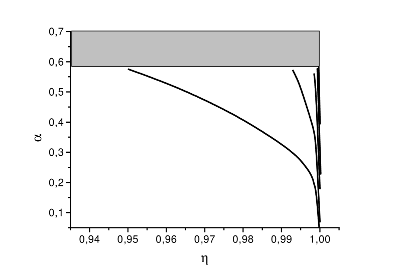
Figure 11: Solutions of the BS equation (4) for constituents of equal mass. The parameters are defined as $\alpha=e^{2}/4\pi$ and $\eta=M/(m_{1}+m_{2})$. The lines represent discrete solutions and the shaded area stands for a continuum of solutions. We took 40 meshpoints for the momentum-integration which lead to a lower bound of $\alpha\approx 0.59$ for the continuum.

We turn to the case of rather weakly bound states of the electron and the positron (weakly bound equal mass case). The results are shown in fig. 11. The lines represent discrete solutions which start at $\alpha\approx 0$ as well as at greater values of $\alpha$ and the shaded area marks the beginning of a continuum of solutions. Since we took 40 meshpoints for the standard calculations the continuum starts at $\alpha\approx 0.59$.

For $0<\eta\leq 0.94$ the continuum is the only feature of the spectrum of solutions of the BS equation (4), i.e. the continuum of solutions (which was known to appear for $M\rightarrow 0$) is present for all values of $\eta$, and it is so with a constant lower bound.

The BS equation for scalar constituents and scalar exchange particle gave complex solutions $\alpha(\eta)$ for constituents of different mass and for a massive exchange particle. We solved the BS equation (4) for various mass ratios $m_{1}/m_{2}\neq 1$ and $m_{\gamma}/m_{2}\neq 0$ and the results agree qualitatively with those that have been obtained for the scalar theory. To mention two of the more pronounced features: a massive photon destroys the clustering of solutions at $\alpha=0$ and for $M\rightarrow m_{1}+m_{2}$. As well as for the scalar theory we found complex solutions $\alpha(\eta)$ which, however, were found only above the lower bound of the continuum.

Let us finally take up the discussion of the (in-)consistency of the approximations for the propagators and for the kernel that enter the BS equation (4). As for the scalar theory we approximate the loop series $\Gamma_{2}$ by

$$\Gamma_{2} =$$ (57)

$$= \frac{e^{2}}{2}\int d^{4}x\,d^{4}y\,{\mathrm{tr}}\biggl{(}S\left(x,y\right)\gamma^{\mu}S\left(y,x\right)\gamma^{\nu}D_{\mu\nu}\left(x,y\right)\biggr{)}$$

where $S$ and $D_{\mu\nu}$ are the propagators of the electron and the photon, respectively. These propagators are not the corresponding bare propagators but the solution of the coupled system of Dyson-Schwinger equations:

$$\frac{\delta\Gamma}{\delta S}=\frac{\delta\Gamma}{\delta D_{\mu\nu}}=0.$$ (58)

Using the approximation (57) for $\Gamma_{2}$ one may derive the explicit Dyson–Schwinger equations that correspond to (58). This leads to a system of equations which is shown in fig. 12 and which compares to the system of equations for the scalar theory fig. 8.

If the appoximation (57) is used as input for the general form of the BS equation

$$\int d^{4}x^{\prime}\,d^{4}y^{\prime}\,\Gamma_{ik,i^{\prime}k^{\prime}}^{\left(2\right)}\left(x,y;x^{\prime},y^{\prime}\right)\psi^{i^{\prime}k^{\prime}}\left(x^{\prime},y^{\prime}\right)=0$$ (59)

one obtains the ladder approximation to the BS equation which is given in (4). However, it has to be emphasized that the propagators $S$ and $D$ are not the bare ones but the solution of (58).

$\biggl{(}\begin{minipage}{56.9055pt} \psfig{width=56.9055pt} \end{minipage}\biggr{)}^{-1}=\hskip 11.38109pt\biggl{(}\begin{minipage}{56.9055pt} \psfig{width=56.9055pt} \end{minipage}\biggr{)}^{-1}+\hskip 11.38109pt\begin{minipage}{56.9055pt} \psfig{width=56.9055pt} \end{minipage}$

$\biggl{(}\begin{minipage}{56.9055pt} \psfig{width=56.9055pt} \end{minipage}\biggr{)}^{-1}=\hskip 11.38109pt\biggl{(}\begin{minipage}{56.9055pt} \psfig{width=56.9055pt} \end{minipage}\biggr{)}^{-1}+\hskip 11.38109pt\begin{minipage}{56.9055pt} \hskip 5.69046pt \psfig{width=39.83368pt} \end{minipage}$

Figure 12: Graphical representation of the coupled system of Dyson-Schwinger equations (58). Thick and thin lines represent the dressed and the bare propagators, respectively.

For the scalar theory we showed that the physical condition $0\leq Z_{i},Z_{m_{i}}\leq 1$ gives a domain of validity for the system of Dyson–Schwinger equations as well as for the ladder approximation to the BS equation. In order to obtain a first estimate we solved the system of equations in quenched approximation thus effectively neglecting the equation for the photon. The equation for the propagator of the electron is then given by

$$S^{-1}\left(p\right)=Z_{2}\left(p/-m_{0}\right)-iZ_{1}e^{2}\int^{\Lambda}\frac{d^{4}k}{\left(2\pi\right)^{4}}\gamma^{\mu}S\left(k\right)\gamma^{\nu}D_{\mu\nu}\left(k-p\right)$$ (60)

where the bare mass $m_{0}$ as well as the renormalization constants $Z_{1}$ and $Z_{2}$ depend on the renormalization scale $\mu$ and on the cutoff $\Lambda$. As one can read off from (60) the approximation (57) yields the bare fermion–photon vertex together with an obviously nonperturbative propagator for the fermion. This implies that the Ward–Takahashi identity cannot be satisfied, i.e. $Z_{1}=Z_{2}$ cannot be assumed. Since the use of the bare vertex enforces $Z_{1}=1$ we determined only $Z_{2}$ and $m/m_{0}$ according to the renormalization condition

$$\left.S^{-1}\left(p\right)\right|_{p^{2}=0}=p/-m$$ (61)

and fixed $Z_{1}$ to 1. For simplicity we employed the normalization at the soft point $p^{2}=0$ instead of the on–shell renormalization. Defining the scalar functions $A$ and $B$ through the relation

$$S\left(p\right)=\frac{1}{p/A\left(p^{2}\right)-B\left(p^{2}\right)}$$ (62)

one obtains from (60) a coupled system of equations for $A$ and $B$ after taking appropriate combination of traces. In terms of these scalar functions the renormalization conditions read $A(0)=1$ and $B(0)=m$.

The details of the numerical solution are given in appendix E, and therefore we focus on the results. For the physical coupling constant $\alpha=1/137$ the scalar functions $A$ and $B$ are nearly equal to their perturbative limits, i.e. $A\approx 1$ and $B\approx m$, as could be anticipated.

Figure 13: The mass–ratio $m/m_{0}$ versus the coupling constant $\alpha$. The divergence of this quantity signals chiral symmetry breaking.

For greater values of $\alpha$ an increasing number of iterations was needed in order to obtain a self–consistent solution. We found no solution for $\alpha>0.74$ which compares quite well with the critical value $\alpha=\pi/4\approx 0.785$ and with the lower bound of the continuum, which was estimated to be at $\alpha\approx 0.807$. Fig. 13 displays the mass–ratio $m/m_{0}$. The divergence of this quantity signals dynamical generation of a mass for vanishing bare mass, i.e. spontaneous breaking of chiral symmetry. To clarify the significance of this result in comparison to the scalar model we plot in fig. 14 the inverse mass–ratio $m_{0}/m$ and the renormalization constant $Z_{2}$ versus the coupling constant $\alpha$. Both $Z_{2}$ and $m_{0}/m$ change sign at the same value of $\alpha$, $\alpha\approx 0.75$. A commonly accepted interpretation of this is that dynamical chiral symmetry breaking occurs at the critical value of the coupling constant, and that above this value of the renormalized fine structure constant QED is not defined [27, 28].

Figure 14: The renormalization constant $Z_{2}$ and the mass-ratio $m_{0}/m$ versus the coupling constant $\alpha$.

5 Conclusions

The central aim of this investigation was a clarification how (or more precisely, whether) the physical spectrum of excited states may be infered from the fully relativistic Bethe–Salpeter equation. In a very strict sense the answer is negative: Taking into account the need for renormalization in the underlying theory the applicability of the ladder Bethe–Salpeter equation turns out to be very restricted. The comparison to (quenched) QED demonstrates this clearly. It is asserted that the value of renormalized fine structure constant has to be lower than some critical value in order to allow for reasonably behaved quantum field theory, see e.g. [28] for a corresponding result in a Dyson-Schwinger approach and [29] for a lattice calculation. Finding the similar behaviour that the field renormalization constants becomes negative for large couplings one may speculate that our (super–renormalizable) scalar model is also well–defined only for renormalized couplings below the critical one signaled by the zero of the renormalization constant. Below these critical values of the coupling constant the Dyson–Schwinger equations for the propagators as well as the Bethe–Salpeter equation in rainbow–ladder approximation were shown to give physically acceptable solutions only. In addition, the use of bare propagators in the Bethe–Salpeter equation introduces only a small additional error.

For large couplings the homogeneous ladder Bethe–Salpeter equation possesses abnormal solutions being excitations in the relative time coordinate. Half of these abnormal states are odd w.r.t. this relative time, and they lead to complex eigenvalues via the crossing with even states. In addition, in QED there is the problem of a continuum of solutions (Goldstein problem). The investigation reported here provides evidence that all these crazy things happen beyond the applicability region of the underlying renormalized quantum field theory. Thus, before studying a spectrum using the Bethe–Salpeter equation one should ensure oneself that the renormalization of one–particle properties can be performed with a physically acceptable result.

Acknowledgments

We thank Gerhard Hellstern for discussions and contributions in the early stages of this work and Martin Oettel for a critical reading of the manuscript and his comments. Furthermore, we thank Lorenz von Smekal for helpful discussions. We are grateful to Hugo Reinhardt for encouragement and support.

This work has been supported by BMBF under contract 06TU888.

Appendix

Appendix A Numerical method for the solution of the scalar Bethe–Salpeter equation

The Wick–rotated homogeneous BS equation for scalar constituents and scalar exchange particle is given by

$$\chi\left(\bar{p},\bar{P}\right)=g^{2}\frac{1}{\bar{p}_{1}^{2}+m_{1}^{2}}\frac{1}{\bar{p}_{2}^{2}+m_{2}^{2}}\int\frac{d^{4}\bar{p}^{\prime}}{\left(2\pi\right)^{4}}\frac{\chi\left(\bar{p}^{\prime},\bar{P}\right)}{\left(\bar{p}-\bar{p}^{\prime}\right)^{2}+\mu^{2}}\,,$$ (63)

where the euclidean momenta $\bar{p}_{i}$ are defined according to

$$\bar{p}_{1}:=\alpha\bar{P}+\bar{p},\quad\bar{p}_{2}:=(1-\alpha)\bar{P}-\bar{p}.$$ (64)

The symmetries of this equation have been discussed in section 1.2 and are summarised in table 1. For a massless exchange particle (63) is invariant under $O(4)$ transformations and the BS amplitudes are proportional to a spherical harmonic of $SO(4)$, denoted by $Z_{klm}$. In the case of $O(3)$ angular momentum $l=0$ the $Z_{klm}$ are proportional to Gegenbauer polynomials $C_{k}^{1}$ of degree 1, see [30] for their definition. For a massive exchange particle the $O(4)$-symmetry is only approximate. Nevertheless, it turns out that the expansion

$$\chi\left(\bar{p},\bar{P}\right)=\sum_{m=0}^{\infty}C_{m}^{1}\left(\cos\left(\theta\right)\right)\chi_{m}\left(\left\|\bar{p}\right\|,\left\|\bar{P}\right\|\right)\quad\quad\theta:=\sphericalangle\left(\bar{p},\bar{P}\right)$$ (65)

still converges very fast. For further usage we now define the dimensionless “momenta”

$$x:=\frac{\|\bar{p}\|}{m_{2}},\quad x^{\prime}:=\frac{\|\bar{p}^{\prime}\|}{m_{2}},\quad$$ (66)

the dimensionless mass-parameters

$$\delta:=\frac{m_{1}}{m_{2}},\quad\kappa:=\frac{\mu}{m_{2}},\quad\eta:=\frac{M}{m_{1}+m_{2}},$$ (67)

and the dimensionless coupling constant

$$\lambda:=\frac{g^{2}}{16\pi^{2}m_{2}^{2}}\,.$$ (68)

Furthermore the abbreviations

$$z:=\frac{\kappa^{2}+x^{2}+x^{\prime 2}}{2xx^{\prime}},\quad B:=z-\sqrt{z^{2}-1}$$ (69)

will be used. The integration over the euclidean momentum $\bar{p}^{\prime}$ is done in spherical coordinates:

$$\int d^{4}\bar{p}^{\prime}=\int_{0}^{\infty}d\bar{p}^{\prime}\bar{p}^{\prime 3}\int_{0}^{\pi}d\theta^{\prime}\sin^{2}\theta^{\prime}\int_{0}^{\pi}d\varphi^{\prime}\sin\varphi^{\prime}\int_{0}^{2\pi}d\psi^{\prime}\,,\quad\quad\theta^{\prime}:=\sphericalangle\left(\bar{p}^{\prime},\bar{P}\right).$$ (70)

The integrations over $\theta^{\prime},\varphi^{\prime},\psi^{\prime}$ can be done analytically and the integral over the absolute value of $\bar{p}^{\prime}$ has been mapped to the interval $[-1,+1]$ according to

$$x^{\prime}=\tan(\frac{\pi}{4}(1+z))\quad\int_{0}^{\infty}dx^{\prime}\rightarrow\frac{\pi}{4}\int_{-1}^{+1}\frac{dz}{\cos^{2}\left(\frac{\pi}{4}\left(1+z\right)\right)}$$ (71)

for the numerical $z$-integration

$$\int_{-1}^{+1}dzf(z)\quad\rightarrow\quad\sum_{j=1}^{N_{1}}w_{z}(j)f(z_{j}).$$ (72)

$w_{z}(j)$ are hereby the weights of the Gauss-Legendre integration. After projection onto the expansion coefficients $\chi_{k}$ we arrive at an eigenvalue problem for the coupling constant $\lambda$

$$\phi_{k}\left(x_{i},\eta\right)=\lambda\sum_{n=0}^{N_{2}}\sum_{j=1}^{N_{1}}A_{ki,nj}\cdot\phi_{n}\left(x_{j},\eta\right)\,,$$ (73)

where the auxiliary functions $\phi_{k}:=i^{k}x^{2}\chi_{k}(\bar{p},\bar{P})$ have been used. The indices $n$ and $i$ run over the degree of the Gegenbauer polynomial and over the $N_{1}$ mesh points for the momentum integration, respectively. The definition of the matrix $A_{ki,nj}$ is given by

$$A_{ki,nj} := \frac{\pi}{4}\frac{1}{\delta\eta^{2}x_{i}}\frac{1}{y_{1}+y_{2}}\frac{w_{z}\left(j\right)}{\cos^{2}\left(\frac{\pi}{4}\left(1+z_{j}\right)\right)}\frac{\left[-i^{k-n-1}S_{nk}\right]}{n+1}B^{n+1},$$ (74)

$$y_{1} := \frac{\delta\left(1-\eta^{2}\right)+x_{i}^{2}}{2\delta\eta x_{i}},\quad\quad y_{2}:=\frac{1-\eta^{2}+x_{i}^{2}}{2\eta x_{i}},$$ (75)

$$S_{nk} := \frac{\left(-1\right)^{n}}{i^{k-n-1}}\left(\frac{\left(-1\right)^{\sigma+k+n}A_{1}^{\left|n-k\right|+1}+A_{1}^{n+k+3}}{1+A_{1}^{2}}\right.,$$ (76)

$$\quad\quad\quad\quad\quad+\left.\frac{\left(-1\right)^{\sigma}A_{2}^{\left|n-k\right|+1}-\left(-1\right)^{n+k+1}A_{2}^{n+k+3}}{1+A_{2}^{2}}\right),$$ (77)

$$\sigma := \frac{1}{2}\left(\left|n-k\right|+k+n\right),$$ (78)

$${\rm and}$$ (79)

$$A_{i} := y_{i}-\sqrt{y_{i}^{2}+1}\,.$$ (80)

Different LAPACK-routines have been used to solve the eigenvalue problem (73) and to cross-check the results.

Appendix B The Bethe–Salpeter amplitudes for euclidean momenta an for constituents of equal mass

The BS amplitudes describing a bound state of scalar constituents of equal mass are defined by

$$\chi\left(x_{1},x_{2},P\right) = \left\langle 0\left|T\left\{\Phi\left(x_{1}\right)\Phi\left(x_{2}\right)\right\}\right|P\right\rangle$$ (81)

$$\overline{\chi}\left(x_{1},x_{2},P\right) = \left\langle 0\left|T\left\{\Phi^{\dagger}\left(x_{1}\right)\Phi^{\dagger}\left(x_{2}\right)\right\}\right|P\right\rangle$$

$$= \left\langle 0\left|\overline{T}\left\{\Phi\left(x_{1}\right)\Phi\left(x_{2}\right)\right\}\right|P\right\rangle^{*}$$

where $T$ is the usual time ordering operator and $\overline{T}$ denotes time ordering in the reverse order. Now we use the definitions

$$X = \alpha x_{1}+(1-\alpha)x_{2}$$ (83)

$$x = x_{1}-x{2}$$

to separate the center of mass motion

$$\chi\left(x_{1},x_{2};P\right)=e^{-iP\cdot X}\,\phi\left(x,P\right)$$ (84)

defining thereby $\phi$, which denotes the relative part of the BS amplitude. Taking this separation of the center of mass and writing the time ordering explicitely we obtain

$$\chi\left(x_{1},x_{2},P\right) = e^{-iP\cdot X}\left(\Theta\left(x^{0}\right)g\left(x,P\right)\,+\Theta\left(-x^{0}\right)g\left(-x,P\right)\,\right)$$ (85)

$$\overline{\chi}\left(x_{1},x_{2},P\right) = e^{iP\cdot X}\left(\Theta\left(x^{0}\right)g\left(-x,P\right)\,+\Theta\left(-x^{0}\right)g\left(x,P\right)\right)^{*}\,.$$ (86)

Since we assumed constituents of equal mass we may take the amplitudes to have a definite $x_{0}$-parity $\epsilon\left(\phi\right)$ which is defined by

$$\phi\left(-x^{0},\mathbf{x}\right)=\epsilon\left(\phi\right)\,\phi\left(x^{0},\mathbf{x}\right)\,.$$ (87)

This can be used to rewrite eqs. (85),(86) in the following way

$$\phi\left(x_{1},x_{2},P\right) = \left(\Theta\left(x^{0}\right)g\left(x,P\right)\,+\Theta\left(-x^{0}\right)g\left(-x,P\right)\,\right)\,,$$ (88)

$$\overline{\phi}\left(x_{1},x_{2},P\right) = \,\epsilon\left(\phi\right)\,\left(\Theta\left(x^{0}\right)g\left(-x^{0},\mathbf{x},P\right)\,+\Theta\left(-x^{0}\right)g\left(x^{0},-\mathbf{x},P\right)\right)^{*}\,.$$ (89)

Using the relation

$$\Theta\left(z\right)=-\frac{1}{2\pi i}\int dk\,e^{-ikz}\,\frac{1}{k+i0^{+}}$$ (90)

we find the following Fourier-transforms

$$\int d^{4}x\,e^{-ip\cdot x}\Theta\left(x^{0}\right)g\left(x,P\right) = -\frac{1}{2\pi i}\int dq^{0}\,\frac{\widetilde{g}\left(q^{0},\mathbf{p},P\right)}{q^{0}-p^{0}+i0^{+}}\,,$$ (91)

$$\int d^{4}x\,e^{-ip\cdot x}\Theta\left(-x^{0}\right)g\left(-x,P\right) = -\frac{1}{2\pi i}\int dq^{0}\frac{\widetilde{g}\left(q^{0},-\mathbf{p},P\right)}{q^{0}+p^{0}+i0^{+}}\,,$$

$$\int d^{4}x\,e^{-ip\cdot x}\Theta\left(x^{0}\right)\left[g\left(-x^{0},\mathbf{x},P\right)\right]^{*} = -\frac{1}{2\pi i}\int dq^{0}\frac{\widetilde{g}^{*}\left(q^{0},-\mathbf{p},P\right)}{q^{0}-p^{0}+i0^{+}}\,,$$

$$\int d^{4}x\,e^{-ip\cdot x}\Theta\left(-x^{0}\right)\left[g\left(x^{0},-\mathbf{x},P\right)\right]^{*} = -\frac{1}{2\pi i}\int dq^{0}\frac{\widetilde{g}^{*}\left(q^{0},\mathbf{p},P\right)}{q^{0}+p^{0}+i0^{+}}$$

which may be used to rebuild the Fourier transforms of the relative part $\phi$ of the BS amplitudes. After Wick-rotation $p_{0}\rightarrow ip_{4}$ we find the relation

$$\widetilde{\overline{\phi}}\left(\bar{p},P\right)=\epsilon\left(\phi\right)\left[\widetilde{\phi}\left(\bar{p},P\right)\right]^{*}$$ (92)

for the relative parts of the BS amplitudes and for euclidean relative momenta $\bar{p}$.

Appendix C Numerical method for the solution of the Dyson-Schwinger equations of the scalar theory

The coupled system of DS equations for the propagators of the scalar fields $\Phi_{i}\,,i=1,2,3$, is given by

$$\Sigma_{i}\left(p^{2}\right) = \Delta_{i}+Z_{i}2g^{2}i\int\frac{d^{4}q}{\left(2\pi\right)^{4}}\,G_{3}\left(p-q\right)G_{i}\left(q\right)\,,\quad\quad i=1,2\,,$$ (93)

$$\Sigma_{3}\left(p^{2}\right) = \Delta_{3}+g^{2}i\int\frac{d^{4}q}{\left(2\pi\right)^{4}}\,\sum_{i=1}^{2}Z_{i}G_{i}\left(p-q\right)G_{i}\left(q\right)$$ (94)

where the abbreviation

$$\Delta_{i}:=\left(1-Z_{i}\right)p^{2}+\left(Z_{i}Z_{m_{i}}-1\right)m_{i}^{2}\,,\qquad i=1,2,3\,,$$ (95)

and the definition $\Sigma_{i}(p^{2}):=p^{2}-m_{i}^{2}-G_{i}^{-1}(p)$ have been used. For notational convenience we introduce

$$F_{ik}(p^{2}):=\int\frac{d^{4}q}{(2\pi)^{4}}G_{i}(p-q)G_{k}(q)\,,\quad\quad i,k=1,2,3\,,$$ (96)

which allows to rewrite the equations (93),(94) in the form

$$\Sigma_{i}\left(p^{2}\right) = \left(1-Z_{i}\right)p^{2}+\left(Z_{i}Z_{m_{i}}-1\right)m_{i}^{2}+Z_{i}2g^{2}iF_{3i}(p^{2})\,,\quad\quad i=1,2\,,$$ (97)

$$\Sigma_{3}\left(p^{2}\right) = \left(1-Z_{3}\right)p^{2}+\left(Z_{3}Z_{m_{3}}-1\right)m_{3}^{2}+g^{2}i\sum_{i=1}^{2}Z_{i}F_{ii}(p^{2})\,.$$ (98)

We use the on-shell renormalization condition $\Sigma_{i}\left(m_{i}^{2}\right)=0$ to eliminate $Z_{m_{i}}$ and obtain

$$\Sigma_{i}\left(p^{2}\right) = (1-Z_{i})(p^{2}-m_{i}^{2})+Z_{i}2g^{2}i\biggl{(}F_{3i}(p^{2})-F_{3i}(m_{i}^{2})\biggr{)}\,,\quad i=1,2\,,$$ (99)

$$\Sigma_{3}\left(p^{2}\right) = (1-Z_{3})(p^{2}-m_{3}^{2})+g^{2}i\sum_{i=1}^{2}Z_{i}\biggl{(}F_{ii}(p^{2})-F_{ii}(m_{3}^{2})\biggr{)}\,.$$ (100)

The $F_{ik}$ contain the self–energies $\Sigma_{i}\left((p-q)^{2}\right)$ and $\Sigma_{k}\left(q^{2}\right)$. In the following we use an angle approximation, i.e. we substitute $\max(q^{2},p^{2})$ for $(p-q)^{2}$ if (and only if) $(p-q)^{2}$ appears as the argument of $\Sigma_{i}\,,\,i=1,2,3$. After Wick-rotation

$$q=(q_{0},\mathbf{q})\rightarrow(iq_{4},\mathbf{q})=:\bar{q}$$ (101)

we change to spherical coordinates

$$\int d^{4}\bar{q}\rightarrow\int_{0}^{\Lambda_{UV}}d\bar{q}\bar{q}^{3}\int_{0}^{\pi}d\theta\sin^{2}\theta\int_{0}^{\pi}d\varphi\sin\varphi\int_{0}^{2\pi}d\psi$$ (102)

where we temporarily introduced the cutoff $\Lambda_{UV}$. Because of the angle approximation the integrations over $\theta,\varphi$ and $\psi$ can be done analytically which leads to

$$F_{ik}=\frac{i}{32\pi^{2}p^{2}}\int_{0}^{\Lambda}d\bar{q}^{2}\frac{\sqrt{c^{2}+4\bar{p}^{2}\bar{q}^{2}}-c}{\bar{q}^{2}+m_{k}^{2}+\Sigma_{k}(-\bar{q}^{2})}\,,$$ (103)

where the abbreviation

$$c:=-\bar{p}^{2}+\bar{q}^{2}+m_{i}^{2}+\Sigma_{i}\left(-\max(\bar{p}^{2},\bar{q}^{2})\right)$$ (104)

has been used for convenience. The system of equations has been solved iteratively and in each step of the iteration the field renormalization constants $Z_{i}$ are calculated according to

$$\left.\frac{d}{dp^{2}}\Sigma(p^{2})\right|_{p^{2}=m^{2}}=0\,.$$ (105)

The solutions $\Sigma_{i}\,,\,i=1,2,3\,,$ of the system of equations (93) and (94) enter the BS equation via the propagators of the constituents and the exchange particle, see equation (44) and its derivation. More explicitely:

$$\psi^{12}\left(p,P\right)=\alpha g^{2}iG_{1}\left(p_{1}\right)G_{2}\left(p_{2}\right)\int\frac{d^{4}q}{\left(2\pi\right)^{4}}\frac{\psi^{12}\left(q,P\right)}{\left(p-q\right)^{2}+m_{3}^{2}+\Sigma_{3}\left(\left(p-q\right)^{2}\right)}$$ (106)

where

$$p_{1}:=p-\alpha P\,,\quad p_{2}:=p+(1-\alpha)P$$ (107)

and

$$G_{i}\left(p_{i}\right)=\frac{1}{p_{i}^{2}+m_{i}^{2}+\Sigma_{i}\left(p_{i}^{2}\right)}\,,\quad\quad i=1,2\,.$$ (108)

This equation is no longer an eigenvalue problem for the square of the coupling constant $g^{2}$. However, one may introduce a formal eigenvalue $\alpha$ and regard $g$ and $M$ as parameters. A solution, i.e. a pair $(g,M)$ is now signaled by the eigenvalue $\alpha=1$. Since we use the angle approximation it is sufficient to apply the substitution $m_{i}^{2}\rightarrow m_{i}^{2}+\Sigma_{i}(p^{2}_{\max})$ to the eigenvalue problem as given in (73) and the following equations in order to obtain the corresponding eigenvalue problem with self–energies taken into account.

Appendix D Numerical method for the solution of the Bethe–Salpeter equation for QED

The BS equation for positronium is given by

$$\Gamma\left(q,P\right)=-i\frac{g^{2}}{\left(2\pi\right)^{4}}\int d^{4}k\,D^{\mu\nu}\left(q-k\right)\gamma_{\mu}G_{1}\left(k_{+}\right)\Gamma\left(k,P\right)G_{2}\left(k_{-}\right)\gamma_{\nu}\,.$$ (109)

The propagators of the constituents and the corresponding momenta are defined according to

$$G_{i}\left(p\right)=\frac{p\diagup+m_{i}}{p^{2}-m_{i}^{2}+i\epsilon}\,,\quad\quad\begin{tabular}[]{l}$k_{+}:=k+\alpha_{1}P$\\ $k_{-}:=k-\alpha_{2}P$\end{tabular}\,,\begin{tabular}[]{l}$\alpha_{1}+\alpha_{2}=1$\end{tabular}\,,$$ (110)

where we allowed for different masses of the electron and the positron. Since all the calculations have been done in the Feynman gauge we used

$$D_{\mu\nu}\left(p\right)=\frac{g_{\mu\nu}}{p^{2}+i\epsilon}\,,$$ (111)

$$\Gamma\left(q,P\right)=\gamma_{5}\biggl{(}\Gamma_{1}\left(q,P\right)+\left(P\cdot q\right)q\diagup\Gamma_{2}\left(q,P\right)+P\!\diagup\Gamma_{3}\left(q,P\right)\biggr{)}\,,$$ (112)

for the propagator of the photon and for the vertex function. (For discussion and references see section 4.) As for the scalar theory we use Gegenbauer expansions for the scalar functions $\Gamma_{k}$

$$\Gamma_{k}\left(\bar{q},\bar{P}\right)=\sum_{i=0}^{\infty}C_{i}^{1}\left(\cos\theta\right)\left[\Gamma_{k}\right]_{i}\left(\left\|\bar{q}\right\|,\left\|\bar{P}\right\|\right)\,,\quad\theta:=\sphericalangle\left(\bar{q},\bar{P}\right)\,,$$ (113)

as well as for the propagators of the constituents and the photon. Applying appropriate combinations of traces and projections one obtains a coupled system of equations for the coefficients $\left[\Gamma_{k}\right]_{i}$ of the Gegenbauer expansion (113). After Wick-rotation $p=(p_{0},{\bf p})\rightarrow(ip_{4},{\bf p})=:\bar{p}$ this system of equations reads

$$\left[\Gamma_{1}\right]_{i} = \frac{g^{2}}{\left(2\pi\right)^{3}}\frac{-1}{\alpha_{1}\alpha_{2}\left(\delta+1\right)^{2}x\eta^{2}}\int\overline{d^{3}y}\,{\sf P}_{i}\sum_{i^{\prime}=0}^{\infty}C_{i^{\prime}}^{1}\left(\cos\theta_{k}\right)S_{3}S_{2}S_{1}$$

$$\quad\quad\quad\quad\quad\quad\quad\quad\quad\quad\quad\,\,\left(A_{11}\left[\Gamma_{1}\right]_{i^{\prime}}+A_{12}\left[\Gamma_{2}\right]_{i^{\prime}}+A_{13}\left[\Gamma_{3}\right]_{i^{\prime}}\right)\,,$$

$$\left[\Gamma_{2}\right]_{i} = \frac{g^{2}}{\left(2\pi\right)^{3}}\frac{-1}{\alpha_{1}\alpha_{2}\left(\delta+1\right)^{2}x\eta^{2}}\int\overline{d^{3}y}\,{\sf P}_{i}\sum_{i^{\prime}=0}^{\infty}C_{i^{\prime}}^{1}\left(\cos\theta_{k}\right)S_{3}S_{2}S_{1}\frac{1}{f_{2}}$$

$$\quad\quad\quad\quad\quad\left(\,\,\,\,\left[i\left(\delta+1\right)\left(\eta x\cos\theta\right)A_{21}-\left(\delta+1\right)^{2}\eta^{2}A_{31}\right]\left[\Gamma_{1}\right]_{i^{\prime}}\right.$$

$$\quad\quad\quad\quad\quad+\left[i\left(\delta+1\right)\left(\eta x\cos\theta\right)A_{22}-\left(\delta+1\right)^{2}\eta^{2}A_{32}\right]\left[\Gamma_{2}\right]_{i^{\prime}}$$

$$\quad\quad\quad\quad\quad+\left.\,\,\left[i\left(\delta+1\right)\left(\eta x\cos\theta\right)A_{23}-\left(\delta+1\right)^{2}\eta^{2}A_{33}\right]\left[\Gamma_{3}\right]_{i^{\prime}}\right)\,,$$

$$\left[\Gamma_{3}\right]_{i} = \frac{g^{2}}{\left(2\pi\right)^{3}}\frac{-1}{\alpha_{1}\alpha_{2}\left(\delta+1\right)^{2}x\eta^{2}}\int\overline{d^{3}y}\,{\sf P}_{i}\sum_{i^{\prime}=0}^{\infty}C_{i^{\prime}}^{1}\left(\cos\theta_{k}\right)S_{3}S_{2}S_{1}\frac{1}{f_{3}}$$

$$\quad\quad\quad\quad\quad\left(\,\,\,\,\left[-\left(\delta+1\right)^{2}\eta^{2}A_{31}-x^{2}A_{21}\right]\left[\Gamma_{1}\right]_{i^{\prime}}\right.$$

$$\quad\quad\quad\quad\quad+\left[-\left(\delta+1\right)^{2}\eta^{2}A_{32}-x^{2}A_{22}\right]\left[\Gamma_{2}\right]_{i^{\prime}}$$

$$\quad\quad\quad\quad\quad+\!\left.\left[-\left(\delta+1\right)^{2}\eta^{2}A_{33}-x^{2}A_{23}\right]\left[\Gamma_{3}\right]_{i^{\prime}}\,\,\,\,\right)\,,$$

In addition to the dimensionless mass–parameters

$$\eta=\frac{M}{m_{1}+m_{2}},\quad\delta=\frac{m_{1}}{m_{2}}\,,$$ (117)

and the dimensionless “momenta”

$$x=\frac{\left\|\bar{q}\right\|}{m_{2}}\,,\quad y=\frac{\left\|\bar{k}\right\|}{m_{2}}\,,$$ (118)

several abbreviations have been used:

$${\sf P}_{i}=\frac{2}{\pi}\int_{0}^{\pi}d\theta\,\sin^{2}(\theta)\,C_{i}^{1}\left(\cos\theta\right)\quad\Rightarrow\quad{\sf P}_{i}C_{k}^{1}(\cos\theta)=\delta_{ik}\quad,$$ (119)

$$\int\overline{d^{3}y}=\int_{0}^{\infty}dy\,\int_{0}^{\pi}d\theta_{k}\sin^{2}\theta_{k}\int_{0}^{\pi}d\varphi_{k}\sin\varphi_{k}\quad,$$ (120)

$$S_{1} = \sum_{n_{1}=0}^{\infty}C_{n_{1}}^{1}\left(\cos\theta_{k}\right)\left[g_{1}-\sqrt{g_{1}^{2}-1}\right]^{n_{1}+1},$$ (121)

$$S_{2} = \sum_{n_{2}=0}^{\infty}\left(-1\right)^{n_{2}}C_{n_{2}}^{1}\left(\cos\theta_{k}\right)\left[g_{2}-\sqrt{g_{2}^{2}-1}\right]^{n_{2}+1},$$ (122)

$$S_{3} = \sum_{n_{3}=0}^{\infty}C_{n_{3}}^{1}\left(\cos\theta_{k}\right)\left[g_{3}-\sqrt{g_{3}^{2}-1}\right]^{n_{3}+1},$$ (123)

$$g_{1}=i\frac{y^{2}-\alpha_{2}^{2}\left(\delta+1\right)^{2}\eta^{2}+1}{2\alpha_{2}\left(\delta+1\right)y\eta}\,,\quad g_{2}=i\frac{y^{2}-\alpha_{1}^{2}\left(\delta+1\right)^{2}\eta^{2}+\delta^{2}}{2\alpha_{1}\left(\delta+1\right)y\eta},$$ (124)

$$g_{3}=\frac{x^{2}+y^{2}}{2xy},$$ (125)

$$f_{2} = -i\left(\delta+1\right)^{3}\left(\eta x\cos\theta\right)\left[\left(\eta x\cos\theta\right)^{2}+\eta^{2}x^{2}\right],$$ (126)

$$f_{3} = \left(\delta+1\right)^{2}\left(-x^{2}\left(\delta+1\right)^{2}\eta^{2}+\left(\eta x\cos\theta\right)^{2}\right),$$

$$A_{11} = 4\left(y^{2}-i\left(\alpha_{1}-\alpha_{2}\right)\left(\delta+1\right)\left(\eta y\cos\theta_{k}\right)+\alpha_{1}\alpha_{2}\left(\delta+1\right)^{2}\eta^{2}+\delta\right),$$ (127)

$$A_{12} = 4i\left(\delta+1\right)\left(\eta y\cos\theta_{k}\right)\left(\left(1-\delta\right)y^{2}-i\left(\alpha_{1}+\alpha_{2}\delta\right)\left(\delta+1\right)\left(\eta y\cos\theta_{k}\right)\right),$$

$$A_{13} = 4\left(i\left(\delta^{2}-1\right)\left(\eta y\cos\theta_{k}\right)-\left(\alpha_{1}+\alpha_{2}\delta\right)\left(\delta+1\right)^{2}\eta^{2}\right),$$

$$A_{21} = -2i\left(\delta^{2}-1\right)\left(\eta y\cos\theta_{k}\right)+2\left(\alpha_{1}+\alpha_{2}\delta\right)\left(\delta+1\right)^{2}\eta^{2},$$

$$A_{22} = i\left(\delta+1\right)\left(\eta y\cos\theta_{k}\right)\left(2i\left(-y^{2}+\alpha_{1}\alpha_{2}\left(\delta+1\right)^{2}\eta^{2}-\delta\right)\left(\delta+1\right)\left(\eta y\cos\theta_{k}\right)\right.$$

$$\quad\quad\quad\quad\quad\quad\quad\quad\quad\quad+2\left(\alpha_{2}-\alpha_{1}\right)y^{2}\left(\delta+1\right)^{2}\eta^{2}$$

$$\quad\quad\quad\quad\quad\quad\quad\quad\quad\quad\left.-4i\alpha_{1}\alpha_{2}\left(\delta+1\right)^{3}\eta^{2}\left(\eta y\cos\theta_{k}\right)\right),$$

$$A_{23} = -4\left(\delta+1\right)^{2}\left(\eta y\cos\theta_{k}\right)^{2}+2\left(\delta+1\right)^{2}y^{2}\eta^{2}$$

$$\quad\quad\quad\quad\quad\quad\quad\quad\quad\quad+2i\left(\alpha_{1}-\alpha_{2}\right)\left(\delta+1\right)^{3}\eta^{2}\left(\eta y\cos\theta_{k}\right)$$

$$\quad\quad\quad\quad\quad\quad\quad\quad\quad\quad-2\alpha_{1}\alpha_{2}\left(\delta+1\right)^{4}\eta^{4}-2\delta\left(\delta+1\right)\eta^{2},$$

$$A_{31} = 2\left(\delta-1\right)\left(xy\cos\omega\right)+2i\left(\alpha_{1}+\alpha_{2}\delta\right)\left(x\eta\cos\theta\right)\left(\delta+1\right),$$

$$A_{32} = i\left(\delta+1\right)\left(\eta y\cos\theta_{k}\right)\left(-2\left(-y^{2}+\alpha_{1}\alpha_{2}\left(\delta+1\right)^{2}\eta^{2}-\delta\right)\left(xy\cos\omega\right)\right.$$

$$\quad\quad\quad\quad\quad\quad\quad\quad\quad\,\,\,\,\,\,+2i\left(\alpha_{2}-\alpha_{1}\right)\left(\delta+1\right)y^{2}\left(x\eta\cos\theta\right)$$

$$\quad\quad\quad\quad\quad\quad\quad\quad\quad\quad+\left.4\alpha_{1}\alpha_{2}\left(\delta+1\right)^{2}\left(\eta y\cos\theta_{k}\right)\left(x\eta\cos\theta\right)\right),$$

$$A_{33} = -4i\left(\delta+1\right)\left(\eta y\cos\theta_{k}\right)\left(xy\cos\omega\right)+2i\left(\delta+1\right)y^{2}\left(x\eta\cos\theta\right)$$

$$\quad\quad\quad\quad\quad\quad\quad\quad\quad\quad-2\left(\alpha_{1}-\alpha_{2}\right)\left(\delta+1\right)^{2}\eta^{2}\left(xy\cos\omega\right)$$

$$\quad\quad\quad\quad\quad\quad\quad\quad\quad\quad-2i\alpha_{1}\alpha_{2}\left(\delta+1\right)^{3}\eta^{2}\left(x\eta\cos\theta\right)$$

$$\quad\quad\quad\quad\quad\quad\quad\quad\quad\quad-2i\delta\left(\delta+1\right)\left(x\eta\cos\theta\right),$$

$$\theta:=\sphericalangle\left(\bar{q},\bar{P}\right),\quad\theta_{k}:=\sphericalangle\left(\bar{k},\bar{P}\right),\quad\omega:=\sphericalangle\left(\bar{q},\bar{k}\right).$$

As for the scalar BS equation we used the transformation (71) to map the integration over the absolute value $\|\bar{k}\|$ to the range $[-1,+1]$. The integrations over $\|\bar{k}\|$ (corresponding to $z$ after the transf. (71) ) and over the angles $\theta_{k},\varphi_{k},\theta$ have been performed with the Gauss-Legendre quadrature. Finally one obtains an eigenvalue problem for the square of the coupling constant which can formally written as

$$\frac{1}{g^{2}}\left(\begin{array}[]{l}\Gamma_{1}\\ \Gamma_{2}\\ \Gamma_{3}\end{array}\right)=\left(\begin{array}[]{lll}B_{11}&B_{12}&B_{13}\\ B_{21}&B_{22}&B_{23}\\ B_{31}&B_{32}&B_{33}\end{array}\right)\left(\begin{array}[]{l}\Gamma_{1}\\ \Gamma_{2}\\ \Gamma_{3}\end{array}\right).$$ (128)

The $B_{ik}$ are matrices of dimension $N_{1}\left(N_{2}+1\right)\times N_{1}\left(N_{2}+1\right)$ where $N_{1}$ is the number of mesh points that have been used for the momentum integration over $z$ and $N_{2}$ is the maximal degree of Gegenbauer polynomials that have been taken into account.

Appendix E Details of the numerical solution of the Dyson-Schwinger equation for the electron propagator

Using the definition

$$S\left(p\right)=\frac{1}{p\diagup A\left(p^{2}\right)-B\left(p^{2}\right)}$$ (129)

of the scalar functioins $A$ and $B$ the DS equation (60) translates into

$$A\left(p^{2}\right)p\diagup+B\left(p^{2}\right) = Z_{2}\left(p\diagup-m_{0}\right)$$

$$+ iZ_{1}e^{2}\int^{\Lambda}\frac{d^{4}k}{\left(2\pi\right)^{4}}\left(\frac{-2A\left(k^{2}\right)k\diagup+4B\left(k^{2}\right)}{A^{2}\left(k^{2}\right)k^{2}-B^{2}\left(k^{2}\right)}\right)\frac{1}{\left(p-k\right)^{2}}$$

Applying $\frac{1}{4}tr\left(\quad\right)$ and $\frac{1}{4}tr\left(\gamma^{\mu}\quad\right)$ leads to separate but coupled equation for the scalar functions $A$ and $B$. After Wick-rotation $p=(p_{0},{\bf p})\rightarrow(ip_{4},{\bf p})=:\bar{p}$ the coupled system of equations for $A$ and $B$ reads

$$A\left(-\bar{p}^{2}\right)=Z_{2} + \frac{Z_{1}e^{2}}{8\pi^{2}}\frac{1}{\bar{p}^{4}}\int_{0}^{\bar{p}^{2}}d\bar{k}\,\bar{k}^{5}\frac{A\left(-\bar{k}^{2}\right)}{A^{2}\left(-\bar{k}^{2}\right)\bar{k}^{2}+B^{2}\left(-\bar{k}^{2}\right)}$$

$$+ \frac{Z_{1}e^{2}}{8\pi^{2}}\int_{\bar{p}^{2}}^{\Lambda^{2}}d\bar{k}\,\bar{k}\frac{A\left(-\bar{k}^{2}\right)}{A^{2}\left(-\bar{k}^{2}\right)\bar{k}^{2}+B^{2}\left(-\bar{k}^{2}\right)},$$

$$B\left(-\bar{p}^{2}\right)=Z_{2}m_{0} + \frac{Z_{1}e^{2}}{2\pi^{2}}\frac{1}{\bar{p}^{2}}\int_{0}^{\bar{p}^{2}}d\bar{k}\,\bar{k}^{3}\frac{B\left(-\bar{k}^{2}\right)}{A^{2}\left(-\bar{k}^{2}\right)\bar{k}^{2}+B^{2}\left(-\bar{k}^{2}\right)}$$

$$+ \frac{Z_{1}e^{2}}{2\pi^{2}}\int_{\bar{p}^{2}}^{\Lambda^{2}}d\bar{k}\,\bar{k}\frac{B\left(-\bar{k}^{2}\right)}{A^{2}\left(-\bar{k}^{2}\right)\bar{k}^{2}+B^{2}\left(-\bar{k}^{2}\right)}$$

where now all the momenta are euclidean.

In order to derive eqs. (E) and (E) we used the relations

$$\int d\Omega_{4}\frac{1}{\left(\bar{p}-\bar{k}\right)^{2}} = 2\pi^{2}\left[\Theta\left(\bar{k}^{2}-\bar{p}^{2}\right)\frac{1}{\bar{k}^{2}}+\Theta\left(\bar{p}^{2}-\bar{k}^{2}\right)\frac{1}{\bar{p}^{2}}\right]$$ (133)

$$\int d\Omega_{4}\frac{\bar{p}\cdot\bar{k}}{\left(\bar{p}-\bar{k}\right)^{2}} = \pi^{2}\left[\Theta\left(\bar{k}^{2}-\bar{p}^{2}\right)\frac{\bar{p}^{2}}{\bar{k}^{2}}+\Theta\left(\bar{p}^{2}-\bar{k}^{2}\right)\frac{\bar{k}^{2}}{\bar{p}^{2}}\right]$$ (134)

where

$$\int d\Omega_{4}:=\int_{0}^{\pi}d\theta_{k}\,\sin^{2}\theta_{k}\int_{0}^{\pi}d\varphi_{k}\,\sin\varphi_{k}\int_{0}^{2\pi}d\psi_{k}.$$ (135)

The wave function renormalization constant $Z_{2}$ and the mass ratio $m/m_{0}$ have been fixed according to

$$A(0)=1\,,\quad B(0)=m.$$ (136)

and the vertex renormalization $Z_{1}$ has been set equal to $1$, for a discussion of this point see section 4.

We took an exponential distribution of mesh points $\bar{k}_{i}$ and used an extended formula of order $O(1/N^{3})$ to perform the momentum integrations, see [31].

References

• [1] E. E. Salpeter and H. A. Bethe, Phys. Rev. 84 (1951), 1232.
• [2] M. Gell–Mann and F. Low, Phys. Rev. 84 (1951), 350.
• [3] J. Schwinger, Proc. Nat. Acad. Sci., 37 (1951), 452; 455.
• [4] F. J. Dyson, Phys. Rev., 75 (1949), 1736.
• [5] G. C. Wick, Phys. Rev., 96 (1954), 1124.
• [6] R. E. Cutkosky, Phys. Rev. 96 (1954), 1135.
• [7] N. Nakanishi, Suppl. Prog. Theor. Phys. 43 1 (1969), 1.
• [8] T. Nieuwenhuis and J. A. Tjon, Few-Body Systems 21 (1996), 167.
• [9] F. L. Scarf, Phys. Rev. 100 (1955), 912.
• [10] Y. Ohnuki, K. Watanabe, Suppl. Progr. Theor. Phys. (1965), 416.
• [11] W. B. Kaufmann, Phys. Rev. 187 (1969), 2951.
• [12] I. Fukui and N. Setô, Progr. Theor. Phys. 89 (1993), 205.
• [13] I. Fukui and N. Setô, hep-ph/9509382
• [14] J. Bijtebier, Nucl. Phys. A623 (1997), 498.
• [15] M. Ciafolini, Nuo. Cim., 51 A (1967), 1090.
• [16] N. Nakanishi, in: Proc. Int. Symp. on Extended Objects and Bound Systems, Karuizawa, Japan, 1992; Eds.: O. Hara, S. Ishida and S. Naka, World Scientific, Singapore 1992; p 109.
• [17] S. Naito, N. Nakanishi, Prog. Theor. Phys. 42 (1969), 402
• [18] M. Ida, Prog. Theor. Phys. 43 (1970), 184
• [19] N. Nakanishi, Phys. Rev. 138, B 1182 (1965) N. Nakanishi, Phys. Rev., 139, B 1401 (1965)
• [20] R. E. Cutkosky, M. Leon, Phys. Rev., 135, B 1445 (1964)
• [21] J. M. Cornwall, R. Jackiw, E. Tomboulis, Phys. Rev., D10, 2428 (1974)
• [22] R. Rosenfelder, A. W. Schreiber, Phys. Rev., D53, 3337, (1996) R. Rosenfelder, A. W. Schreiber, Phys. Rev., D53, 3354, (1996)
• [23] T. Nieuwenhuis, J. A. Tjon, Phys. Rev. Lett., 77, 814, (1996)
• [24] See, e.g., C. D. Roberts and A. G. Williams, Prog. Part. Nucl. Phys. 33, 477 (1994), and references therein.
• [25] C. H. Llewellyn Smith, Ann. Phys., 53, 521 (1969)
• [26] J. S. Goldstein, Phys. Rev., 91, 1516 (1953)
• [27] “Dynamical Symmetry Breaking in Quantum Field Theories”, V. A. Miranski, World Scientific, 1993; and references therein.
• [28] F. T. Hawes, T. Sizer, and A. G. Williams, Phys. Rev., D55, 3866 (1997); and references therein
• [29] M. Göckeler, R. Horsley, V. Linke, G. Schierholz, H. Stüben, Phys. Rev. Lett., 80, 4119 (1998)
• [30] M. Abramowitz and I. A. Stegun, Handbook of Mathematical Functions, Dover, New York, 1965
• [31] W. H. Press, S. A. Teukolsky, W. T. Vetterling, B. P. Flannery, “Numerical Recipes in Fortran”, 2nd edition, Cambridge University Press, section 4.1