© 1998 International Press
Adv. Theor. Math. Phys. 2 (1998) 1405 –1439
Non-Supersymmetric Conformal
Field Theories from Stable
Anti-de Sitter Spaces
††footnotetext: e-print archive: http://xxx.lanl.gov/abs/hep-th//9810206
††footnotetext: Work supported in part by NSF Grant PHY9511632 and
the Robert A. Welch††footnotetext: Foundation.
Jacques Distler and Frederic Zamora
Theory Group, Physics Department
University of Texas at Austin
Austin TX 78712 USA.
distler@golem.ph.utexas.edu
zamora@zerbina.ph.utexas.edu
Abstract
We describe new non-supersymmetric conformal field theories in three and four dimensions, using the CFT/AdS correspondence. In order to believe in their existence at large and strong ’t Hooft coupling, we explicitly check the stability of the corresponding non-supersymmetric anti-de Sitter backgrounds. Cases of particular interest are the relevant deformations of the SCFT in and invariant directions. It turns out that the former is a stable, and the latter an unstable non-supersymmetric type IIB background.
1 Introduction
Two dimensional conformal field theories exhibit a very rich structure, and much can be said about their properties. One of the most striking features is the ability to control, not just the conformal theory itself, but also the nearby nonconformal theories obtained by adding certain specially-chosen relevant perturbations. These nonconformal theories exhibit a structure (exact-integrability) almost as rich as that of their conformal cousins. Moreover, one can actually follow these perturbations and see how the theory flows from the ultraviolet fixed point CFT to a new fixed point (a different conformal field theory) in the infrared.
Not so much is known about conformal field theories in higher dimensions. The richest information, to date, has only come for supersymmetric conformal field theories.
Recently, however, a new avenue to understanding conformal field theories (in various dimensions) has opened up. The CFT/AdS correspondence [1] gives a precise quantitative relation [2, 3] between a conformal field theory in dimensions, and a solution to string theory/M-theory on a background of the form , with compact. At least for large (and large ), the latter is computable, in that it is well-approximated by a classical supergravity calculation.
In this paper, we would like to imitate the construction which was very successful in two dimensions, and construct new conformal field theories by taking known examples from the CFT/AdS correspondence, perturbing them by relevant operators, and flowing to the infrared. In favourable circumstances, we will find that the perturbed theory indeed flows to a new conformal field theory in the infrared.
In our examples, the perturbation breaks some or all of the supersymmetry. Hence, we will, in particular, be learning about new, non-supersymmetric conformal field theories. This is exciting, in itself, as there are not too many known examples of such for . We will find examples of these non-supersymmetric CFTs in and discuss the case of .
The downside of breaking supersymmetry is that self-consistency of the supergravity solution is no longer assured, even at the classical level. If a tachyonic scalar in anti-de Sitter space has a negative mass-squared which exceeds the Freedman-Breitenlohner stability bound [4, 5, 6], leads to an expo-nentially-growing mode, rendering the supergravity solution unstable. Super-symmetry ensures that there are no such unstable modes in a supersymmetry-preserving solution to the supergravity equations. It, plausibly, also takes care that quantum corrections do not upset the classical solution. (We say, plausibly, as no one actually knows how to compute quantum corrections in these Ramond-Ramond backgrounds.) In the non-supersymmetric case, we will actually have to check the stability, even at the classical level by hand. We will also restrict ourselves to the large limit, where quantum corrections are parametrically small (being down by factors of ) and do not upset the large solution.
We will study in greatest detail the relevant deformations of the SCFT. Those relevant operators are mapped to the scalars in supergravity multiplet, whose dynamics is encoded in the five dimensional gauged supergravity Lagrangian [7]. In particular, in §3, we follow the renormalization group flow of the SYM with the addition of a mass term for one of the gluinos. Such a term breaks all the supersymmetries and the R-symmetry to . We will see the existence of a non-supersymmetric invariant background of type IIB string theory, smoothly connected (via the VEV of the scalar field in the supergravity corresponding to the gaugino mass) with the usual BPS invariant background. We will see the relation between the supergravity solution which interpolates between these asymptotic behaviours and RG flow in the field theory, perturbed by this -invariant relevant operator. We compute the mass spectrum of the low-lying states in this -invariant supergravity solution (equivalently, we find the conformal dimension of the corresponding operators in the CFT), and check that it is, indeed, a stable solution.
In §4 we analyse another kind of relevant deformation of the SYM: a quadratic term for one of the adjoint scalars. This term also breaks supersymmetry, and leaves an subgroup of unbroken. As before, its ultraviolet relevant coupling constant connects the maximally supersymmetric type IIB background to a non-supersymmetric background (with now being an squashed five-sphere in one direction, breaking the isometries to ). Unfortunately, this supergravity background proves to be unstable. So, in this case, there is no corresponding -invariant CFT.
§5 deals with conformal field theories. We review some invariant fixed points studied by Warner [8], and observe the existence of a non-supersymmetric invariant fixed point, connected to the invariant fixed point by an appropriate renormalization group flow.
Finally, in §6, we discuss the relevant deformation of the SCFT, breaking supersymmetry and the R-symmetry group to . As in the invariant theory, this deformation ends up in an unstable supergravity background. We also check the stability of a non-supersymmetric M-theory background [9], which was recently proposed as leading to a non-supersymmetric, invariant, CFT in . This theory, too, turn out to be unstable.
After this work was completed, we received the preprint [10], which overlaps with material of §3,4. They also noted the existence of the and invariant type IIB backgrounds and their connection to conformal field theories on the boundary. Unfortunately, they did not compute the spectrum of masses around these new critical points and so could not check the stability of these solutions.
2 Relevant Deformations of , SCFT
The CFT/AdS correspondence can be extended to particular non-super-symmetric relevant directions of the SCFT. At large and strong ’t Hooft coupling, the deformed theory is given by the solution of the classical equations of motion of the gauged supergravity action in , with boundary conditions determined by the relevant couplings.
There are two type of relevant deformations: by superconformal primaries
| (2.1) |
with being the six real scalars in the adjoint of and in the of ; and by superconformal primaries
| (2.2) |
with being Weyl spinors in the adjoint of and in the of . These deformations give, respectively, supersymmetry-breaking masses to the scalars and to the gluinos.
The and are in the and of , respectively. These, plus the two singlet marginal couplings tr and tr, are associated to the scalars of the supergravity multiplet in . To study the field theory deformed by these relevant couplings, we need to study the dynamics of the supergravity theory with these scalars turned on.
The ungauged , supergravity Lagrangian has global symmetry and local symmetry , where is the maximal compact subgroup of . The previous 42 scalars are described by an element of the coset space which transforms in the of (acting on the indices from the left) and of (acting on the indices from the right) 111The ( ) of is the traceless, antisymmetric tensor representation, , . After gauging the subgroup of , a nontrivial scalar potential is generated. It is proportional to the square of the gauge coupling, , and breaks down to [7]. We will use an subgroup of as a basis to represent the 42 scalars into (the indices are restricted to be indices ) 222The reference [7] chose the subgroup of as the basis to perform the gauging of . As we will see, the complex basis described here is more convenient for studying of the deformations; and the real basis is more suited for the deformations.. In the unitary gauge, only the physical scalars remain in the matrix , with . The scalars transform in the irreducible , , of The acts on the of by . The gauge group and the compact generator of are embedded in this , with the following branching rules:
| (2.3) |
where the subscript denotes the charge. Ordering the dimensional vector space by , the can be written in block form
| (2.4) |
where the is the representation of .
The supergravity scalar potential is built from the quantities [7]:
| (2.5a) | ||||
| (2.5b) | ||||
where is the symplectic metric and
is the -invariant, skew-symmetric,
bilinear quadratic form
acting on
. The final expression for the potential is 333 indices are raised and lowered with the symplectic metric .
| (2.6) |
Then, the scalar plus graviton sector of the gauged supergravity Euclidean Lagrangian (in appropriate Planck units) is described by the following non-linear sigma model coupled to gravity:
| (2.7) |
3 The Non-Supersymmetric -Invariant Theory
As a first step in exploring the non-supersymmetric theories connected to the fixed point, one can study the theory in the -invariant direction given by the relevant deformation:
| (3.1) |
The relevant coupling has UV scaling mass dimension one and it gives a mass term only to the gaugino . Supersymmetry is completely broken and the R-symmetry is broken to a global symmetry. It is useful to keep track of the factor, a linear combination of the and the , which is unbroken by this perturbation (but which is broken by the VEV of the dilaton).
To study the theory along this invariant direction, we decompose the representations discussed above under :
| (3.2) |
Together with (2.3), we can identify all the operators in the different representations. They can also be derived from their microscopic field content. The four gluinos decompose as () and . The six scalars can be combined into complex combinations , which transform as the . The relevant perturbation is in the singlet representation , so that it is left invariant by the factor generated by the charge .
Now we turn to the supergravity description of this non-supersymmetric invariant theory. Only the two complex scalars corresponding to the singlet representations have boundary conditions different from the trivial ones, as the only couplings which are turned on on the field theory side are , and . The (complex) field, corresponding to the non-compact generators of (the dilaton and the axion), do not appear in the potential because of the invariance of the tensor (2.5a). We write this complex field as a modulus times a phase, . The other complex scalar, , is associated to the complex coupling . The phase is eaten via the Higgs mechanism, and, in a unitary gauge, only the modulus enters in the coset element . We order the representations in the by
In this basis, it proves convenient to parametrize as
| (3.3) |
where,
| (3.4) |
Plugging this into the supergravity Lagrangian (2.7), one gets
| (3.5) |
where , and
| (3.6) |
The classical gauge coupling has been determined to be in order to have anti-de Sitter radius at the supersymmetric point .
Note that the metric for and is invariant, as it should be. Weak string coupling corresponds to .
As already mentioned, the phase of is eaten by the Higgs mechanism. It is not a modulus. On the field theory side, this corresponds to the fact that the phase of can be removed by a chiral rotation of the gluinos (i.e. absorbed by a shift in the angle).
3.1 The equations of motion
Now, we just have to solve the equations of motion for subject to the boundary conditions as :
| (3.7) |

The boundary conditions are translationally invariant along the four dimensional Euclidean space . Therefore, we consider the ansatz
| (3.8) |
with for . In fact, the equations of motion and the boundary conditions only depend of the dimensionless combination , therefore the field solutions only depend on this parameter . Furthermore, one can show that the equations of motion do not admit a zero of (which would yield a singularity of the metric). Hence we can redefine the coordinate such that and the boundary conditions (3.7) are still satisfied. Finally one ends up with the equations (prime means derivative with respect to ):
| (3.9a) | ||||
| (3.9b) | ||||
| (3.9c) | ||||
| (3.9d) | ||||
| (3.9e) | ||||
The dilaton and axion equations are homogeneous, and are easily solved by taking , . There remain three equations for two unknown functions, and . But one can prove that one of them is a consequence of the others two, and the system admits a solution.
Solving the equations of motion (3.9a)–(3.9e) for any gives the behavior of the deformed field theory for any value of . In general, the spacetime metric will not be anti-de Sitter, and the boundary theory is not conformally invariant for finite .
But there is an interesting phenomenon in the asymptotic behavior of the spacetime metric. This behavior is quite easy to obtain from the equations of motion. For , the solution becomes
| (3.10) |
where , and
| (3.11) |
This result requires some explanation.
The scalar potential has two critical points where (see fig. 1). One is at and it is a maximum of the potential. It gives an space, with radius , coming from the compactification of type IIB on , which preserves all the supersymmetries of type IIB. On the 4D field theory side, it corresponds to the invariant superconformal field theory.
The other critical point is located at and it is where the solution for ends up. One can see that for , the theory does not have invariant Killing spinors [7], so supersymmetry is completely broken. We can look at the infinitesimal solution (3.7) and the asymptotic solution (3.10) as the solution driven for and , respectively, and general coordinate . Keeping the external probe energies fixed, these limits correspond to the ultraviolet and infrared limits, respectively. Then, the critical point at is associated to an infrared fixed point of the SYM deformed theory by the -invariant relevant deformation (3.1).
By performing the coordinate transformation
| (3.12) |
the asymptotic solution of the metric becomes
| (3.13) |
with
| (3.14) |
i.e., anti-de Sitter space, but with a smaller radius than the one in the ultraviolet, . The proportionality factor is given by the ratio of the two corresponding cosmological constants (3.11). As the bulk theory is again (Euclidean) anti-de Sitter, just with smaller radius, we have isometry for that metric, yielding conformal invariance for the boundary field theory in the infrared.
The critical point corresponds to a type IIB background AdS, with a stretched five-sphere [11], and the anti-de Sitter radius being . This background breaks all the supersymmetries and the compact manifold has the isometry group .
3.2 The Wilson loop
For general , we have a deformed metric of the type
| (3.15) |
Now consider a Nambu-Goto string action propagating in that deformed 5D space, with the world-sheet boundary attached at . This computes the expectation value of a Wilson loop in the boundary theory [12, 13]. We will consider the static and symmetric Wilson loop
with
such that is the maximum distance reached by the string.
This gives the quark and anti-quark energy potential
| (3.16) |
evaluated through the geodesic. Observe that we are dealing with a classical mechanics problem: the movement of a particle in one dimension with initial point at and end point at . The conserved “particle energy” is
| (3.17) |
where .
If we move the end point , , the quark and anti-quark energy changes as
| (3.18) |
So, the force between the quark and the anti-quark is given by the “particle energy”. We want to read this force for . In order do it, we need the relation between and . From (3.17) one gets
| (3.19) |
where .
The major contribution to the integral is at . One can evaluate the integral in that region, taking , such that . The result is
| (3.20) |
with
| (3.21) |
This gives the relation, for ,
| (3.22) |
For , the force between electric sources becomes
| (3.23) |
It is a nontrivial result that the asymptotic behavior of the deformed metric gives a Coulomb potential. This is another indication that the infrared theory is conformally-invariant. However, at this stage, it might well turn out to be a free theory. One indication that it is not free is that the Peskin exponent 444At a second order phase transition for a gauge theory in dimensions, [14]. at the theory:
| (3.24) |
with given by the integral (3.21), does not vanish, as one expects for a free theory.
We can make additional checks of the Coulomb behavior. We should also see the same kind of potential for magnetic sources. We can test that, computing the minimal area expanded by a D1 brane attached to the boundary , which gives a ’t Hooft loop. The D1 action is
| (3.25) |
where is the dilaton. It gives the same force between magnetic sources, up to an additional dilaton dependent factor,
| (3.26) |
For and being the unique solution of (3.9a)–(3.9e), with the asymptotic behavior (3.10), is an exact solution of the equations of motion with the appropriate boundary conditions. Then, the force between two monopoles becomes
| (3.27) |
Taking into account that , one gets exactly the same force as the one between electric sources, but with the Yang-Mills coupling inverted: . This result is consistent with the electric-magnetic duality of the Coulomb phase.
As an additional check, we can compute the normalized solutions of the dilaton equation for . The eigenvalues give the masses of the intermediate states in the two point correlation function of the operator [15]. The equation is
| (3.28) |
For , one chooses the normalizable solution . For , the normalizable asymptotic behavior is , with . The equation (3.28) gives
| (3.29) |
with unique solution for and . As the smooth deformation by does not change the topology of the five-dimensional spacetime, there are no non-zero square-integrable solutions in the deformed metric.
3.3 The nontrivial fixed point and the stability of supergravity solution
The Coulombic behaviour of the Wilson loop that we found in the previous subsection is indicative of the conformal invariance of the infrared theory. But it is compatible with the infrared theory being a free conformal theory. More exciting would be a nontrivial interacting conformal theory. In the presence of supersymmetry, a wealth of such four dimensional conformal field theories are known, e.g. the Argyres-Douglas points of QCD [16], the QCD in the conformal window [17] and, of course, the SYM, both at the origin of the moduli space. More recently, non-supersymmetric conformal field theories have been proposed as orbifolds of these in the CFT/AdS point of view [18]. We will presently see that the solution we found in the previous subsections is a nontrivial interacting fixed point without supersymmetry.
At we are at the fixed point. As we increase , we go away from that fixed point. For we will end up on a new fixed point. Sending can be seen as going to the infrared, as we saw by introducing the dimensionless variable .
In §3.1 we derived, for
| (3.30a) | ||||
| (3.30b) | ||||
| (3.30c) | ||||
There are two ways to look at this:
-
1)
for fixed, it gives the infrared behavior (that sends );
-
2)
for , it is the solution of the equations of motion for any (and also for any in the field theory side).
Taking the second point of view, it is better to work in terms of the coordinates defined in (3.12). The 4D field theory lives at the boundary . Following the standard procedure as in [2], one gets that for an scalar field with mass at the point, its behavior for is
| (3.31) |
with the larger root of the equation
| (3.32) |
The boundary field value couples to a conformal operator which has the scaling mass dimension
| (3.33) |
In general this gives anomalous dimensions, a sure sign that the fixed point is nontrivial. If were equal to , we would get the same formulae as in the fixed point. But for this invariant fixed point. The scaling dimensions of the operators will be different than they were in the supersymmetric point – first because the masses at the new extremum of the supergravity potential are different, and second because is different. We have already seen that the mass of has changed. At the supersymmetric point, it was tachyonic (the corresponding operator in the 4-dimensional SCFT is relevant). At the point, has positive mass-squared, and the corresponding operator is irrelevant (see fig. 2).
In fact, we will commonly obtain irrational anomalous dimensions (see tables 1 and 2 below). As we are dealing with a non-supersymmetric CFT, the erstwhile chiral primaries (whose scaling dimensions were protected in the supersymmetric theory, and equal to their free field values) are no longer protected. Observe also that we need to have real solutions for (3.32). This is also the bound for vacuum stability in a five-dimensional AdS background with radius [2, 4]. An unstable supergravity solution does not correspond to a sensible CFT on the boundary, as the scaling dimensions corresponding to the unstable modes are complex. So, both from the point of view of checking the stability of the non-supersymmetric solution to the 5D supergravity equations, and to extract the physics of the purported new fixed point, we need to compute the complete quadratic dependence of the supergravity potential in all the scalars fields.
For the parametrization of the coset space , it is convenient to choose one that gives canonical kinetic terms. We take
| (3.34) |
with given by (3.3). The hermitian matrix contains the fluctuations of the remaining tachyonic (at ) scalars. We parametrize them by the following fields: a hermitian and traceless matrix for the representation; symmetric and complex matrices and for the and representations, respectively; and a complex three vector for the . The vectors , are eaten by the Higgs mechanism (along with the phase of ). So, in a unitary gauge, they are absent from the scalar potential. The rest of the fields appear in as
| (3.35) |
where the bar means complex conjugation and .
The broken generators give rise to massive bosons in the of . The masses are easily computed as a function of :
| (3.36) | ||||
The aforementioned 7 scalars from the become the longitudinal components of these massive bosons.
With the parametrization (3.34) 555We work to quadratic order in the fluctuations of , and , but to all orders in , and ., the kinetic terms for the remaining scalars become:
| (3.37) |
Then, we can read directly the masses from the quadratic terms in the potential. We have ():
| (3.38) |
We observe that all the fields satisfy the stability bound of the critical point (see table 1 for their corresponding conformal dimensions). So the non-supersymmetric type IIB background is a stable solution (at least at large and ). It defines a non-supersymmetric interacting infrared fixed point of the invariant theory.
To close this discussion of the infrared fixed point, in table 2 we give the conformal dimensions of the scaling operators corresponding to the remaining modes in the 5D supergravity multiplet (their mass terms are given in [7]). The graviton is mapped to the energy-momentum tensor of the invariant CFT. The eight gravitini (in the of ) map to the four complex supersymmetry currents . The twelve ‘self-dual’ 2-forms (in the ) correspond to the operators [19]
| (3.39) |
The global currents are . At the point, the currents and are not conserved, and pick up anomalous dimensions.
| CFT operator | Supergravity field | ||
|---|---|---|---|
| CFT operator | |
|---|---|
Finally, there are the spin- scaling operators:
| (3.40) |
in the and of , respectively. These correspond to the 48 symplectic Majorana spinors of the five-dimensional supergravity multiplet. At the non-supersymmetric point, eight of them are eaten by the gravitini. This phenomenon is manifested in the CFT by the anomalous dimensions of the broken supersymmetry currents (see table 2)
4 The Invariant Theory
Having succeeded in finding a new nontrivial critical point when the relevant perturbation is turned on, we now try turning on, instead, the relevant perturbation,
| (4.1) |
This gives a positive mass-squared to , and formal negative mass-squared to the scalars . Supersymmetry is completely broken and is broken to .
Decomposing the scalars in the supergravity under ,
| (4.2) |
and the and of both become the ( ) of . The perturbation we are describing corresponds to turning on the singlet scalar, which we will call , in the .
Since all of the representations of that we encounter are real, it behooves us to choose a real basis in which to parametrize the coset matrix . The of decomposes as under . In a real basis, the compact is generated by , and a general matrix in the coset takes the form
| (4.3) |
The of is represented by a traceless symmetric matrix, . Let . If we do not also turn on any of the scalars in the , then the coset element is block diagonal,
| (4.4) |
where
Using the general expression (2.6), the potential reads
| (4.5) |
with the symmetric matrix . Observe that does not appear in the potential, as expected.
The singlet scalar associated to the relevant perturbation (4.1) enters in as
The normalization is chosen to have mass at the supersymmetric point . The Lagrangian (2.7) simplifies to:
| (4.6) |
Now, as in the case, we have to solve the equations of motion of subject to the boundary conditions for :
| (4.7) |
The sign convention in (4.7) is to end up at the critical point of the scalar potential (see fig. 3).
| CFT operator | Supergravity field | ||
|---|---|---|---|
| Graviton | 4 | ||
| Gravitini | 7/2 | ||
| Gravitino | 7/2 | ||
| 2-forms | 3 | ||
| 2-forms | 3 | ||
| Gauge bosons | |||
| W bosons | |||
| W boson | |||
| Spinors | |||
| Spinors | |||
| Spinors | |||
| Spinors |
| CFT operator | |
|---|---|
| 4 | |
| 32/9 | |
| 4 | |
| 26/9 | |
| 34/9 | |
All the same remarks on the equations of motion in the previous section apply in this case. It is consistent to take constant solutions for . The same kind of asymptotic behavior for the metric and the scalar as is found, but with the conformal exponent being now . The reason is the same: the scalar potential
has two critical points where (see fig. 3).
One critical point is at and it is a maximum of the potential. It gives an AdS5 space, with radius , coming from the compactification of type IIB on . On the 4D field theory side, it corresponds to the -invariant superconformal vacuum. The 10 dimensional geometry is the familiar one:
| (4.8) |
The anti-de Sitter space and the five sphere have the same radius . The five-form in the internal space is
| (4.9) |
The integral of over is quantized. In appropriate units, it gives the number of D3-branes in the stack, whose near-horizon geometry is given by (4.8).
The other critical point is at . It breaks and all the supersymmetries. It was conjectured in [7] that it corresponds to the compactification of type IIB on the inhomogeneously squashed five sphere [20, 21]:
| (4.10) |
where
| (4.11) |
and the 5-form field strength in the internal space is
| (4.12) |

The relation between the scale , which characterizes the -invariant solution (4.10), (4.12), and the scale , which characterizes the -symmetric solution, is determined by noting that the five-form flux, being quantized, must be preserved along the RG flow. Equating the integrals of (4.9) and (4.12) over , we find
| (4.13) |
Note, however, that this is not the same as the radius , the radius of the infrared in the Einstein frame of the effective 5-dimensional theory. That is determined by normalizing the Einstein-Hilbert term in the 5-dimensional effective action. One takes the 10-dimensional Einstein-Hilbert term in the background metric (4.10), and integrates it over , and compares the result with the 5-dimensional Einstein Hilbert term for the background metric (but with the 5-dimensional determined from the original round metric (4.8)). The integrals over which appear are identical (all powers of the warp factor disappear), and one has the relation
| (4.14) |
Plugging in (4.13), we recover .
This all sounds very promising, but we need to check the stability of this supergravity solution before we can draw any conclusions. As in the case, this requires that we compute the mass-squared of the scalars about the new extremum of the potential. Since we have already computed the potential for the scalars in the of , let us compute their masses first. As we saw, . The singlet is the field that we turned on. Clearly, its mass-squared is positive at the new extremum (fig. 3). The are eaten by the Higgs mechanism in the breaking of . They also have positive mass-squared, as they are the longitudinal components of the massive vector bosons. So we need to worry about the . Unfortunately, that is where trouble looms. The mass-squared of the can be straightforwardly computed from the potential (4.5) and one finds
| (4.15) |
i.e., they violate the stability bound. Put another way, if we assumed that this solution corresponded to a CFT on the boundary, and attempted to compute the conformal dimension of the operator corresponding to the , via
we would find to be complex.
From the supergravity side, there is nothing mysterious here. The invariant supergravity simply does not provide a stable ground state for the theory. Fluctuations, no matter how small, cause it to decay. And, by the same token, a classical solution with the asymptotics (4.7) is similarly destabilized.
With the benefit of hindsight, we should have expected this instability from the form of the perturbation (4.1). Formally, it gives a negative mass-squared to the scalars in the boundary theory. The naivest expectation for the resulting physics of the boundary theory is that it runs off to infinity in field space and has no stable vacuum. This expectation appears to be confirmed by the supergravity analysis.
5 Three Dimensional Conformal Field Theories
The gauge theory living on the world volume of coincident M2 branes has an interacting infrared fixed point that preserves all the supersymmetries [22]. The near horizon geometry of this BPS brane configuration is . At large , the CFT/AdS correspondence solves the three dimensional SCFT through the mapping of its generating functional to the one of gauged supergravity [23] at the invariant background. The local operators of the field theory are conveniently mapped to the Kaluza-Klein spectrum of the supergravity theory [24, 25, 26, 27].
The ‘massless’ supermultiplet that includes the graviton has 70 physical scalars arranged in the of [28, 29]. They parametrize the coset space via a matrix in the 56 dimensional representation of . In the unitary gauge, it is given by
| (5.1) |
where are 35 complex self-dual four-forms ( are indices).
At the supersymmetric invariant point , these 70 scalars are tachyonic. In the SCFT, they are mapped to relevant primary operators. The scalars (the real part of ) correspond to the conformal primaries:
| (5.2) |
and the pseudo-scalars (the imaginary part of ) correspond to the conformal primaries:
| (5.3) |
where and are the microscopic (real) scalars 666They include the dualized vector field. and (Majorana) gauginos, in the irreps and of respectively, of the gauge theory.
Following the same philosophy as in the SYM case, in this section we will discuss the relevant perturbations of the fixed point via the addition of the operators (5.2) and (5.3) to the supersymmetric Lagrangian. The deformation of the theory through these relevant operators is driven by the solution of the classical equations of motion, subject to appropriate boundary conditions for their associated supergravity modes .
As we have already learned in this paper, the renormalization group trajectories of the relevant operators will connect the fixed point to other new fixed points, if the supergravity potential admits additional stable critical points, besides the invariant point at .
5.1 invariant conformal field theories
In [8], Warner performed an exhaustive study of the extrema of the gauged supergravity potential along invariant directions. He found five additional critical points, displayed in table one of [8]. At the level of eleven dimensional supergravity, they correspond to compactifications . The four dimensional anti-de Sitter space ensures conformal invariance for the field theory living at its boundary. The compact seven dimensional manifold depends on the chosen critical point, such that for each one, it breaks a different number of supersymmetries and isometries.
There are three points where all the supersymmetries are broken and the remaining isometries are , and . The stability of the invariant points was checked in [30] and the answer was negative. We do not know if the point is stable or not.
The other two points keep some unbroken supersymmetries, which ensures vacuum stability [4, 31]. Applying the CFT/AdS correspondence for these points, they describe and , invariant three-dimensional superconformal field theories, where the correlation functions are given by the supergravity partition function evaluated at the appropriate background.
5.2 The interacting fixed point
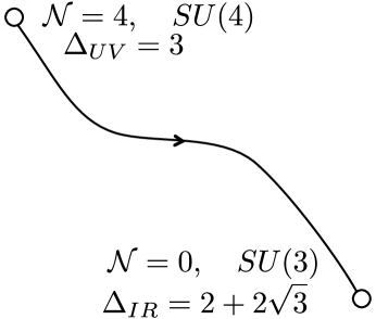
In [31], an invariant critical point was found for the gauged supergravity theory. The interesting thing about this particular point is that it is a non-supersymmetric stable anti-de Sitter background [32], which can be embedded in the theory 777In [32] the stability is only proved for the theory, but it was argued that the result should generalize to the full theory. [33], where the unbroken isometries are . On the field theory side, it corresponds to a new non-supersymmetric interacting fixed point connected to the through some direction in the space of invariant renormalization group trajectories.
Decomposing the representation, first under , and thence under , one obtains:
| (5.4) |
In particular, the singlets transform as a complex scalar in the of . The truncation to the theory consists in setting to zero the scalars in the . Two complex scalars in the can be turned on, breaking to . In the full theory, this breaks to . In the process, 22 of the 70 scalars, the , are eaten by the Higgs mechanism. The remaining scalars are three singlets and five copies of the .
Let us denote the two complex scalars, which are turned on, by , . The supergravity potential reads [33]
| (5.5) |
with and the square of the gauge coupling, which is proportional to the scalar curvature of the anti-de Sitter background at the invariant point .
The scalar potential (5.5) has an additional extremum at
| (5.8) |
The methodology is the same as we learned in the four-dimensional conformal field theories. The conformal structure exponent at the fixed point is different from the one at the SCFT (). This exponent is given by the ratio of the corresponding cosmological constants of the dual supergravity backgrounds at these two critical points. For this case
| (5.9) |
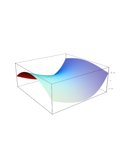
In fig. 4 we plot the scalar potential along two singlet field directions, near the critical point (5.8). As usual, it is a saddle point. In CFT language, the directions with negative (positive) mass-squared are mapped to relevant (irrelevant) operators of the fixed point. From the potential (5.5) and kinetic terms (5.6), we can read off the masses of the scalars at this point. From these, we derive the corresponding scaling dimensions using the formula
| (5.10) |
At the CFT, we have
| (5.11) |
where is the radius at the supersymmetric invariant point and is the mass-squared at the point.
The primary operator that drives the theory from the SCFT to the CFT is associated to the common radial fluctuation and has scaling dimension
| (5.12) |
Its partner, the common phase of the two complex scalars, , is eaten by the Higgs mechanism.
The other two singlet operators continue to be tachyonic at this non-supersymmetric conformal field theory. One is associated to the opposite radial fluctuations , , and has scaling dimension
| (5.13) |
The other corresponds to the relative phase fluctuation , and has scaling dimension
| (5.14) |
6 Six Dimensional Conformal Field Theories
The six dimensional SCFT living on the world volume of coincident M5 branes is described (at large N) by 11D supergravity in the background AdS. The R-symmetry groups is . As in 4 dimensions, one has chiral primary fields, , consisting of order symmetrized traceless products of the scalars in the tensor multiplets (for ). These have scaling dimension . is a relevant operator ) in the of . As in 4 dimensions, we can imagine perturbing the theory by adding this relevant operator to the action, in such a way as to break to .
On the supergravity side, this corresponds to giving a non-trivial boundary conditions for an -singlet scalar in the gauged supergravity multiplet. The construction of the gauged supergravity Lagrangian, up to two derivatives, was done in [34]. The supergravity potential turns out to be equivalent to (4.5), but now with the matrices valued in instead of . As in the AdS5 case, one finds an additional critical point with symmetry, corresponding to a compactification on a squashed . But, as in the AdS5 case, this background is unstable [35]. The scalars in the supergravity multiplet in break up into a singlet, which we are turning on, the , which is higgsed, and the , which violates the stability bound. Indeed, in analogy with what we found in §4, one could have expected that this background would prove unstable. In the boundary theory, the -invariant perturbation gives a positive mass-squared to one of the scalars in the tensor multiplet, and a negative mass-squared to the other four. So one expects this perturbation to cause the boundary theory to run off to infinity in field space, with no stable vacuum.
The other possible four dimensional compact manifold with isometries is . In fact, recently it has been proposed to be a non-supersymmetric stable vacuum of M-theory [9]. Here we perform an explicit check of that statement, computing part of the Kaluza-Klein (KK) mass spectrum that results from that compactification.
For signature and standard Ricci, the Einstein equations of motion are 888 refer to eleven dimensional indices; are internal indices of and correspond to indices in .
| (6.1) |
We work in the Freund-Rubin ansatz:
| (6.2) |
where is a constant proportional to the four-form flux of field strength, created by the presence of M5-branes, through the compact manifold . As it was noted in [9], there is a particular solution with the topology . We choose physical units where . Then, the equations (6.1) determine and the radius-squared of the two to be .
There are three kinds of scalar fields. Two of them come from the fluctuations of the eleven dimensional spacetime metric 999 () means the trace(less) metric fluctuation.
| (6.3a) | |||
| (6.3b) | |||
and the third from the eleven dimensional three-form potential
| (6.4) |
As usual, the internal space dependence is expanded in a basis of tensor harmonics , and of , with their coefficients being the seven dimensional scalar fields. For the case of , these harmonics are a product, , of the harmonics , . The index refer to the irreducible representations , for integer values of and . The masses of the scalar fields and are read from their linearized equations of motion obtained from the variation of (6.1), taking into account expressions (6.3) and (6.4). Since the scalar fluctuations (6.3b) change the volume of , this needs to be compensated by a change in the three-form (6.4) in order to keep the four-form field strength flux constant. The consequence is that the scalars and have mixed mass terms and one should go to an appropiate basis which diagonalize them [36].
On the other hand, the traceless metric fluctuations (6.3a) keep the volume of fixed. Then, it is consistent to consider and constant. Applying this kind of fluctuations to (6.1) for the case of internal indices and , one gets
| (6.5) |
For a general metric fluctuation , in a general background, the fluctuation of the Ricci is (indices are raised and lowered with the background metric)
| (6.6) |
Plugging this in (6.5), it gives the equation (in de Donder gauge, )
| (6.7) |
with the ordinary Laplacian for the metric . Denoting the coordinate indices of the first by letters from the beginning of the Greek alphabet, and the coordinate indices of the second by letters from the end of the Greek alphabet, the curvature tensor of is
| (6.8) |
with all of the mixed components vanishing. This is different from all of the other cases treated in [36], where the curvature tensor takes the form
| (6.9) |
In an earlier version of this paper, we naively applied the subsequent formulæ of [36], which implicitly assume the form (6.9). In some cases, these gives results which agree with (6.8), but in the crucial case of the breather mode, which we discuss below, they do not101010We would like to acknowledge conversations with Berkooz and Rey, which helped us track down the source of our previous error..
Since we are dealing with a product space, there are two kind of scalar modes from the traceless fluctuations (6.3a). One kind correspond to the ‘jiggling’ modes , for each of the two-spheres; i.e., with being traceless for each of the . Their equation of motion are
| (6.10) |
where the mass-squared is
| (6.11) |
are the eigenvalues of the ordinary Laplace operator on the manifold acting on a symmetric and traceless two-tensor harmonic :
| (6.12) |
with because it is a two-tensor harmonic.
The other kind of modes are the ‘breathing’ modes , which are pure-trace from the point of view of each of the two-spheres. They come from the terms in the expansion (6.3a) where and , with being a product of scalar harmonics on each . The mass-squared of this breathing mode is
| (6.13) |
with now , and . In particular, the lowest mode, corresponding to , has the squared mass , which violates the stability bound . Therefore, the non-supersymmetric background is unstable.
Acknowledgements
We acknowledge valuable discussions with L.J. Boya, R. Corrado and W. Fischler. We would also like to thank M. Berkooz and S. J. Rey for discussions of their work, and for pointing out an error in a previous version of this manuscript. F.Z. would like to thank CERN for its support and hospitality, as well as useful discussions with L. Álvarez-Gaumé, J.L.F. Barbón, M. Bremer, C. Gómez and K. Skenderis, during his visit in June.
References
- [1] J. Maldacena, “The large N limit of superconformal field theories and supergravity,” hep-th/9711200.
- [2] E. Witten, “Anti-de Sitter space and holography,” hep-th/9802150.
- [3] S. S. Gubser, I. R. Klebanov, and A. M. Polyakov, “Gauge theory correlators from noncritical string theory,” hep-th/9802109.
- [4] P. Breitenlohner and D. Z. Freedman, “Stability in gauged extended supergravity,” Ann. Phys. 144 (1982) 249.
- [5] L. Mezincescu and P. K. Townsend, “Stability at a local maximum in higher dimensional anti-de Sitter space and applications to supergravity,” Ann. Phys. 160 (1985) 406.
- [6] L. Mezincescu and P. K. Townsend, “Positive energy and the scalar potential in higher dimensional (super)gravity theories,” Phys. Lett. 148B (1984) 55.
- [7] M. Gunaydin, L. J. Romans, and N. P. Warner, “Compact and noncompact gauged supergravity theories in five-dimensions,” Nucl. Phys. B272 (1986) 598.
- [8] N. P. Warner, “Some new extrema of the scalar potential of gauged supergravity,” Phys. Lett. 128B (1983) 169.
- [9] M. Berkooz and S.-J. Rey, “Nonsupersymmetric stable vacua of M theory,” hep-th/9807200.
- [10] L. Girardello, M. Petrini, M. Porrati, and A. Zaffaroni, “Novel local CFT and exact results on perturbations of super Yang Mills from AdS dynamics,” hep-th/9810126.
- [11] L. J. Romans, “New compactifications of chiral supergravity,” Phys. Lett. 153B (1985) 392.
- [12] J. Maldacena, “Wilson loops in large field theories,” Phys. Rev. Lett. 80 (1998) 4859, hep-th/9803002.
- [13] S.-J. Rey and J. Yee, “Macroscopic strings as heavy quarks in large N gauge theory and anti-de Sitter supergravity,” hep-th/9803001.
- [14] M. E. Peskin, “Critical point behavior of the Wilson loop,” Phys. Lett. 94B (1980) 161.
- [15] E. Witten, “Anti-de Sitter space, thermal phase transition, and confinement in gauge theories,” hep-th/9803131.
- [16] P. C. Argyres, M. R. Plesser, N. Seiberg, and E. Witten, “New superconformal field theories in four dimensions,” Nucl. Phys. B461 (1996) 71–84, hep-th/9511154.
- [17] N. Seiberg, “Electric - magnetic duality in supersymmetric nonAbelian gauge theories,” Nucl. Phys. B435 (1995) 129–146, hep-th/9411149.
- [18] S. Kachru and E. Silverstein, “4-d conformal theories and strings on orbifolds,” Phys. Rev. Lett. 80 (1998) 4855, hep-th/9802183.
- [19] S. Ferrara, C. Fronsdal, and A. Zaffaroni, “On supergravity on AdS5 and superconformal Yang-Mills theory,” hep-th/9802203.
- [20] P. van Nieuwenhuizen and N. P. Warner, “New compactifications of ten-dimensional and eleven- dimensional supergravity on manifolds which are not direct products,” Commun. Math. Phys. 99 (1985) 141.
- [21] C. M. Hull and N. P. Warner, “Noncompact gaugings from higher dimensions,” Class. Quant. Grav. 5 (1988) 1517.
- [22] N. Seiberg, “Notes on theories with 16 supercharges,” hep-th/9705117.
- [23] B. de Wit and H. Nicolai, “ supergravity with local invariance,” Phys. Lett. 108B (1982) 285.
- [24] O. Aharony, Y. Oz, and Z. Yin, “M theory on and superconformal field theories,” hep-th/9803051.
- [25] S. Minwalla, “Particles on and primary operators on M2-brane and M5-brane world volumes,” hep-th/9803053.
- [26] R. Entin and J. Gomis, “Spectrum of chiral operators in strongly coupled gauge theories,” hep-th/9804060.
- [27] E. Halyo, “Supergravity on and M branes,” J. High Energy Phys. 04 (1998) 011, hep-th/9803077.
- [28] A. Casher, F. Englert, H. Nicolai, and M. Rooman, “The mass spectrum of supergravity on the round seven sphere,” Nucl. Phys. B243 (1984) 173.
- [29] M. Gunaydin and N. P. Warner, “Unitary supermultiplets of and the spectrum of the compactification of eleven-dimensional supergravity,” Nucl. Phys. B272 (1986) 99.
- [30] B. de Wit and H. Nicolai, “The parallelizing torsion in gauged supergravity,” Nucl. Phys. B231 (1984) 506.
- [31] G. W. Gibbons, C. M. Hull, and N. P. Warner, “The stability of gauged supergravity,” Nucl. Phys. B218 (1983) 173.
- [32] W. Boucher, “Positive energy without supersymmetry,” Nucl. Phys. B242 (1984) 282.
- [33] N. P. Warner, “Some properties of the scalar potential in gauged supergravity theories,” Nucl. Phys. B231 (1984) 250.
- [34] M. Pernici, K. Pilch, and P. van Nieuwenhuizen, “Gauged maximally extended supergravity in seven- dimensions,” Phys. Lett. 143B (1984) 103.
- [35] M. Pernici, K. Pilch, P. van Nieuwenhuizen, and N. P. Warner, “Noncompact gaugings and critical points of maximal supergravity in seven-dimensions,” Nucl. Phys. B249 (1985) 381.
- [36] P. van Nieuwenhuizen, “The complete mass spectrum of supergravity compactified on and a general mass formula for arbitrary cosets ,” Class. Quant. Grav. 2 (1985) 1.