S645.0998

The conformal window in QCD and supersymmetric QCD

Einan Gardi     and    Georges Grunberg

Centre de Physique Théorique de l’Ecole Polytechnique
91128 Palaiseau Cedex, France
email: gardi@cpht.polytechnique.fr,  grunberg@cpht.polytechnique.fr

Abstract
In both QCD and supersymmetric QCD (SQCD) with $N_{f}$ flavors there are conformal windows where the theory is asymptotically free in the ultraviolet while the infrared physics is governed by a non-trivial fixed-point. In SQCD, the lower $N_{f}$ boundary of the conformal window, below which the theory is confining is well understood thanks to duality. In QCD there is just a sufficient condition for confinement based on superconvergence. Studying the Banks-Zaks expansion and analyzing the conditions for the perturbative coupling to have a causal analyticity structure, it is shown that the infrared fixed-point in QCD is perturbative in the entire conformal window. This finding suggests that there can be no analog of duality in QCD. On the other hand in SQCD the infrared region is found to be strongly coupled in the lower part of the conformal window, in agreement with duality. Nevertheless, we show that it is possible to interpolate between the Banks-Zaks expansions in the electric and magnetic theories, for quantities that can be calculated perturbatively in both. This interpolation is explicitly demonstrated for the critical exponent that controls the rate at which a generic physical quantity approaches the fixed-point.

1 Introduction

In multi-flavor QCD, there is a conformal window [1], namely a region of $N_{f}$ values for which the theory is asymptotically free at short distances while the long distance physics is governed by a non-trivial fixed-point. This is a non-Abelian Coulomb phase in which quarks and gluons are not confined.

The upper boundary of the conformal window is determined according to the sign of the $\beta$ function

$$\beta(x)\,\equiv\,\frac{dx}{d\ln(\mu^{2})}\,=\,-\left(\beta_{0}x^{2}+\beta_{1}x^{3}+\cdots\right),$$ (1)

at small coupling $x\equiv\alpha_{s}/\pi$. When the first coefficient of the perturbative $\beta$ function [2],

$$\beta_{0}=\frac{1}{4}\left(\frac{11}{3}N_{c}-\frac{2}{3}N_{f}\right),$$ (2)

changes its sign the theory changes its nature from the asymptotically free phase $r\equiv N_{f}/N_{c}<11/2$, to the infrared free phase $r>11/2$. The transition point in $N_{c}=3$ QCD is at $N_{f}=16.5$. For $r<11/2$ the $\beta$ function is negative for a vanishingly small coupling ($\beta_{0}>0$), but due to the second term which has an opposite sign ($\beta_{1}<0$), $\beta(x)$ reaches a non-trivial zero at some $x_{\hbox{\tiny FP}}\simeq-\beta_{0}/\beta_{1}>0$ [3]. $x_{\hbox{\tiny FP}}$ approaches zero as $r$ approaches $11/2$, and then quarks and gluons are weakly coupled at all scales. Finally, the smallness of $x_{\hbox{\tiny FP}}$ justifies the use of the 2-loop $\beta$ function.

On the other hand, the lower boundary of the conformal window, below which confinement sets in, is much harder to tackle. One approach to confinement, the so-called metric confinement [4], defines confinement as a phase in which transverse gauge field excitations are excluded from the space of physical states which is defined through the BRST algebra. It was shown in [4] that as long as a certain condition is obeyed by the gauge field propagator, metric confinement is implied. This condition is most conveniently expressed in the Landau gauge, namely that the absorptive part of the gluon propagator $D(Q^{2},\mu^{2},g)$ (in this gauge) is superconvergent,

$$\int_{0^{-}}^{\infty}dk^{2}\,\rho(k^{2},\mu^{2},g)\,=\,0,$$ (3)

where $\mu^{2}$ is the renormalization scale and $\rho(k^{2},\mu^{2},g)=(1/\pi)\,{\rm Im}\left\{D(-k^{2},\mu^{2},g)\right\}$.

Assuming analyticity of the gluon propagator $D(Q^{2},\mu^{2},g)$, the superconvergence relation (3) was shown to be a direct consequence of renormalization group invariance, provided $D(Q^{2},\mu^{2},g)$ vanishes faster than $1/Q^{2}$ at large $Q^{2}$. Due to asymptotic freedom, the last condition depends only on the sign of the 1-loop anomalous dimension of the propagator (in the Landau gauge), given by

$$\gamma_{00}=-\frac{1}{4}\left(\frac{13}{6}N_{c}-\frac{2}{3}N_{f}\right).$$ (4)

If $\gamma_{00}$ is negative the superconvergence relation (3) holds.

Thus, in this approach, a sufficient condition for confinement is that $\gamma_{00}<0$ and therefore the lower boundary of the conformal window cannot be lower than $r=13/4$. If superconvergence is also a necessary condition (this has not been shown) then the phase transition should be at $r=13/4$. In $N_{c}=3$ QCD this corresponds to $N_{f}=9.75$, i.e. between 9 and 10 flavors.

A natural question to ask is whether the superconvergence condition necessarily implies that also quarks are confined. To the knowledge of the authors no complete answer has yet been given to this question, although it has been shown that the superconvergence criterion is consistent with a potential that is approximately linear in some intermediate scales [5].

There are several other approaches to study the phase structure of multi-flavor QCD, such as the instanton liquid model [7], the gap equation [6, 8] and computer simulations on the lattice [9, 10]. The new lattice results [10] are inconsistent with old ones [9] and with the superconvergence criterion for confinement: they indicate that the phase where no confinement nor chiral symmetry breakdown occurs, stretches down to $N_{f}=7$, and thus only for $6$ flavors and below QCD appears as a confining theory with chiral symmetry breaking, as we know it in the real world. In spite of these contradicting evidence, we assume in this paper that the bottom of the conformal window is as implied by superconvergence.

Recently the presence of a fixed-point in QCD was studied as a function $N_{f}$ by considering the perturbative $\beta$ function [11, 12]. Three approaches where considered: a direct investigation of the equation $\beta(x)=0$ in physical renormalization schemes [13], the Banks-Zaks expansion [1, 14, 15] and the analyticity structure of the coupling constant.

The direct investigation of zeros in the QCD $\beta$ function in physical schemes [11] shows that at 3-loop, a fixed-point can appear for most effective charges above $N_{f}\simeq 5$. However, presence of a fixed-point at the lower end is very sensitive to higher-loop corrections, and thus cannot be trusted.

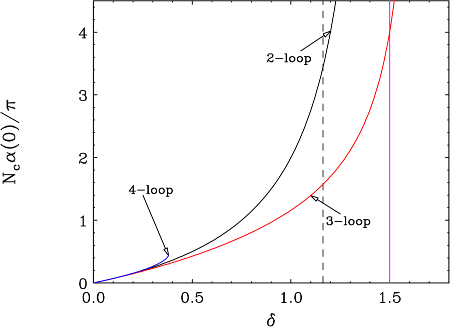
Figure 6: The infrared limit of the 2-loop coupling and the 3-loop and 4-loop DRED couplings in large $N_{c}$ SQCD as a function of $\delta\equiv 3-(N_{f}/N_{c})$. The continuous vertical line represents the bottom of the conformal window implied by superconvergence (or duality) and the dashed vertical line shows the 2-loop causality boundary.

The Banks-Zaks expansion is an expansion in the number of flavors down from the point where $\beta_{0}$ changes its sign. The expansion parameter is proportional to $\beta_{0}$, or in $N_{c}=3$ QCD to $(16.5-N_{f})$. It was found in [11] that Banks-Zaks series for different QCD observables behave differently: in some cases the coefficients are small and the expansion is reliable and in other cases it seems to breakdown at order $(16.5-N_{f})^{3}$ already around 10 or 12 flavors (see fig. 6 in [11]). Here we further interpret these results.

In real-world QCD there are Landau singularities in the perturbative coupling, which signal the inapplicability of perturbation theory to describe the infrared physics. These non-physical singularities are usually assumed to be compensated by non-perturbative power-like terms in any physical quantity. Thus causality is realized only at the non-perturbative level. The existence of a perturbative fixed-point opens up the possibility that the perturbative coupling will have no Landau singularities [11, 12]. We will assume that within the conformal window non-perturbative effects are not important as long as they are not implied by perturbation theory, that is as long as the perturbative coupling is causal and small. Note that the causality requirement is stronger than the requirement to have no space-like Landau singularity.

The simplest example where causality of the coupling can be achieved at the perturbative level, without additional power corrections, is the 2-loop coupling. In [12] an exact explicit formula for the 2-loop coupling as a function of the scale was introduced, which enabled a complete understanding of the singularity structure of the coupling in this approximation. It turns out that the condition for causality of the 2-loop coupling is $c\equiv\beta_{1}/\beta_{0}<-\beta_{0}$. This condition translates in $N_{c}=3$ QCD to $N_{f}\geq 10$.

As stated above the lower boundary of the conformal window implied by superconvergence is also between $9$ and $10$ flavors [4]. Thus basing on the superconvergence criterion, we find that the 2-loop perturbative coupling is causal in the entire conformal window. This suggests that the perturbative analysis in the infrared is reliable down to the bottom of the window. On the other hand, perturbation theory cannot describe the infrared physics in the confining phase. We therefore intend to study more carefully down to what $N_{f}$ can we trust perturbation theory in the infrared, and in particular, when does perturbation theory signal its own inapplicability. The very same questions can be asked also in supersymmetric QCD (SQCD), where more is known about the phase structure. We therefore study here both QCD and SQCD and compare the two.

A few years ago Seiberg lead a revolution in the understanding of supersymmetric gauge theories. Of particular interest to us is the phase structure of $N=1$ SQCD in which non-Abelian electric-magnetic duality plays a major role [16]. The general arguments available in the supersymmetric case do not apply in the absence of supersymmetry and in fact the phase structure of a supersymmetric theory can be quite different from that of its non-supersymmetric parallel [17, 18]. Still the comparison can be very enlightening.

SQCD, just like QCD, has a conformal window where the theory is asymptotically free, and is governed by a non-trivial fixed-point in the infrared. The picture described in [16] is the following: in the upper part of the conformal window the fixed-point value of the coupling is small, and thus the theory is weakly coupled at all scales. The massless fields that appear in the Lagrangian conveniently describe the physics at any scale. When $N_{f}$ becomes smaller (for a fixed $N_{c}$) the theory becomes strongly coupled in the infrared. Then, it does not make sense anymore to describe the physics in terms of the original massless fields. Nevertheless, in the infrared limit the theory has an effective description in terms of a dual theory: starting with an original supersymmetric theory with an $SU(N_{c})$ gauge symmetry and $N_{f}$ massless chiral quark superfields ($Q_{i}$, $i=1,2,...N_{f}$) and their anti-fields ($\tilde{Q}_{i}$, $i=1,2,...N_{f}$) the dual theory is an $SU(N_{f}-N_{c})$ gauge theory with $N_{f}$ chiral quarks superfields ($q_{i}$, $i=1,2,...N_{f}$) and their anti-fields ($\tilde{q}_{i}$, $i=1,2,...N_{f}$), and an additional superpotential describing a Yukawa interaction between color-singlet mesons and the quarks superfields:

$$W=\sqrt{\lambda}\,M_{j}^{i}\,q_{i}\,\tilde{q}^{j}.$$ (5)

The relation between the theories is referred to as duality since the dual of the dual theory is again an $SU(N_{c})$ gauge theory. In the conformal window the dual theory, just like the original one, is asymptotically free and has a non-trivial infrared fixed-point. Contrary to the original theory, the dual theory becomes weakly coupled as $N_{f}$ decreases, until the point where it becomes infrared free. Since the dual theory is weakly coupled when the original one is strongly coupled, and vise-versa, Seiberg refers to this duality as a non-Abelian generalization of the electric-magnetic duality. The duality picture is valid also outside the conformal window, where one of the theories is infrared free and the other is confining, but here we concentrate on the conformal window.

In [19] (see also [20]) it was shown that the lower boundary of the conformal window implied by the superconvergence criterion for confinement in SQCD, coincides with the lower boundary implied by duality which is the point where the dual theory becomes infrared free. This gives additional support to the whole picture, with the advantage that the superconvergence criterion can be applied also in the non-supersymmetric case, as it was originally done in [4, 5].

According to Seiberg’s description, in SQCD the electric theory is strongly coupled at the bottom of the window. We shall demonstrate that this strong coupling behavior manifests itself already at the perturbative level, through appearance of Landau singularities that make perturbation theory inconsistent.

The purpose of the first part of this paper (Sec. 2) is to consider the condition for the perturbative QCD coupling to be causal as a function of $N_{f}$ (for a general $N_{c}$), and compare it with the lower boundary of the conformal window set by superconvergence. In Sec. 2.1 we study causality at the level of the 2-loop coupling and in Sec. 2.2 we examine the effect of higher orders. Next, in Sec. 3, we study the same issue in SQCD. In Sec. 3.1 we investigate the singularity structure of the 2-loop coupling in the electric theory and study the effect of higher orders. In Sec. 3.2 we discuss the dual (magnetic) theory. Sec. 3.3 summarizes the main findings of Sec. 2 and 3. In Sec. 4 we consider the Banks-Zaks expansion for the value of the fixed-point (Sec. 4.1) and for the critical exponent $\gamma$ that controls the rate at which a generic effective charge approaches the fixed-point in the infrared limit (Sec. 4.2). In Sec. 4.3 we show that the 2-point Padé approximants technique [21] can be used to interpolate between the Banks-Zaks expansions for a physical quantity in the two dual theories. The example considered is the critical exponent in the large $N_{c}$ limit.

2 The conformal window in QCD and the analyticity structure of the coupling

As explained in the introduction, according to the superconvergence criterion [4, 5] an $SU(N_{c})$ gauge theory with $N_{f}$ light flavors is confining so long as the anomalous dimension of the gauge field propagator $\gamma_{00}$ of eq. (4) is negative, i.e. for $r=N_{f}/N_{c}<13/4$. This is only a sufficient condition for confinement, and therefore we can expect a phase transition from the confining phase to a phase which is conformally invariant in the infrared, either at $r=13/4=3.25$ or somewhere above this line.

Referring to the superconvergence criterion as determining the lower boundary of the conformal window, we now turn to study the perturbative $\beta$ function. In real-world QCD the perturbative running coupling has “causality violating” Landau singularities on the space-like axis which, according to the common lore, signal the inapplicability of perturbation theory in the infrared region and the necessity of non-perturbative power like terms. On the other hand, close enough to the top of the conformal window causality can be established within the perturbative framework [11, 12]. There the perturbative $\beta$ function leads to a causal running coupling, which has a finite infrared limit and no Landau singularities in the entire $Q^{2}$ plane: its only discontinuity is a cut along the time-like axis. In this situation the perturbative analysis does not signal the need for non-perturbative physics. It is then possible that perturbation theory by itself describes well the infrared physics.

By definition, in the conformal window the coupling reaches a finite limit in the infrared. As explained above, in the upper part of the window this finite limit is obtainable from the perturbative $\beta$ function. Is it true also away from the top of the window? In other words, is it the perturbative coupling that reaches a finite limit? and in this case, can we reliably calculate the fixed-point value in perturbation theory? In order to address these questions we study here the conditions for a causal perturbative coupling and compare them to the boundary of the conformal window.

2.1 Causality from the 2-loop $\beta$ function

The 2-loop $\beta$ function with $\beta_{0}>0$ and $\beta_{1}<0$ is the simplest example where Landau singularities can be avoided, so it is natural to begin by analyzing this example. It should be stressed that the 2-loop $\beta$ function corresponds to a particular choice of renormalization scheme, the so-called ‘t Hooft scheme, where all the higher-order corrections to the $\beta$ function $\beta_{2}$, $\beta_{3}$ and on vanish. Since the first two coefficients of the $\beta$ function are scheme invariant, we shall obtain a criterion for causality which does not have an explicit dependence on the scheme.

The 2-loop renormalization group equation,

$$\beta(x)=\frac{dx}{dt}=-\beta_{0}{x}^{2}\left(1+cx\right)$$ (6)

where $t=\ln(Q^{2}/\Lambda^{2})$, and [3]

$$c\equiv\frac{\beta_{1}}{\beta_{0}}=\frac{1}{16\beta_{0}}\left[\frac{34}{3}N_{c}^{2}+\left(\frac{1}{N_{c}}-\frac{13}{3}N_{c}\right)N_{f}\right]$$ (7)

can be integrated exactly [12] using the Lambert W function [22]. It was shown in [12] that if $c>0$ a Landau branch point is present on the space-like axis, if $-\beta_{0}<c<0$ a pair of Landau branch points appears at some complex $Q^{2}$ values and if

$$c<-\beta_{0}<0$$ (8)

the coupling has a causal analyticity structure, with no Landau singularities. We rederive here these results using a simpler (but less rigorous) approach [23].

Integrating (6) we obtain

$$\ln(Q^{2}/\Lambda^{2})\,=\,\frac{1}{\beta_{0}x}+\frac{1}{\gamma^{2-loop}}\ln\left[\frac{1}{x}-\frac{1}{x_{\hbox{\tiny FP}}}\right]$$ (9)

where $x_{\hbox{\tiny FP}}=-1/c$ and $\gamma^{2-loop}$ is the critical exponent at the 2-loop order. $\gamma$ is defined as the derivative of the $\beta$ function at the fixed point,

$$\gamma\equiv\left.\frac{d\beta(x)}{dx}\right|_{x=x_{\hbox{\tiny FP}}}.$$ (10)

At 2-loop order $\gamma^{2-loop}=-\beta_{0}^{2}/\beta_{1}$.

If $c>0$ there is a Landau singularity on the space-like axis. A positive fixed-point is obtained for $c<0$, but this condition alone does not guarantee causality – there can be Landau singularities in the complex $Q^{2}$ plane.

Assuming that the singularities are such that $|x(Q^{2})|\longrightarrow\infty$, we expand (9) around these points in powers of $1/x$. The leading term in this expansion gives the location of the singularity. The phase of the r.h.s. of (9) at the singularity is

$$\Phi\,=\,\pm\pi\,\frac{1}{\gamma^{2-loop}},$$ (11)

If $|\Phi|<\pi$, i.e. if $\gamma^{2-loop}>1$, or $-\beta_{0}<c<0$, the singularities are in the first sheet (the time-like axis cut corresponds to $|\Phi|=\pi$), and if $|\Phi|>\pi$, i.e. if

$$0<\gamma^{2-loop}<1$$ (12)

or $c<-\beta_{0}$, the 2-loop coupling is causal. The condition (12) (or (8)) for a causal 2-loop coupling translates in QCD into the following condition for $r$ upon substituting $\beta_{0}$ and $c$ from eqs. (2) and (7), respectively:

$$4r^{2}+\left[\frac{9}{N_{c}^{2}}-83\right]r+223<0$$ (13)

This leads to an approximately $N_{c}$ independent critical value for $r$ for any possible value of $N_{c}$ (since $N_{c}^{2}\gg 9/83$), namely the 2-loop coupling is causal as long as

$$r>(83-9\sqrt{41})/8\simeq 3.17.$$ (14)

For lower $r$, the condition (12) does not hold and there appears a pair of complex singularities in the $Q^{2}$ plane. If $r$ is reduced further, $c$ becomes positive and then a Landau branch point appears on the space-like axis. This change occurs at:

$$r=34/\left[13-\frac{3}{N_{c}^{2}}\right]\simeq 2.62.$$ (15)

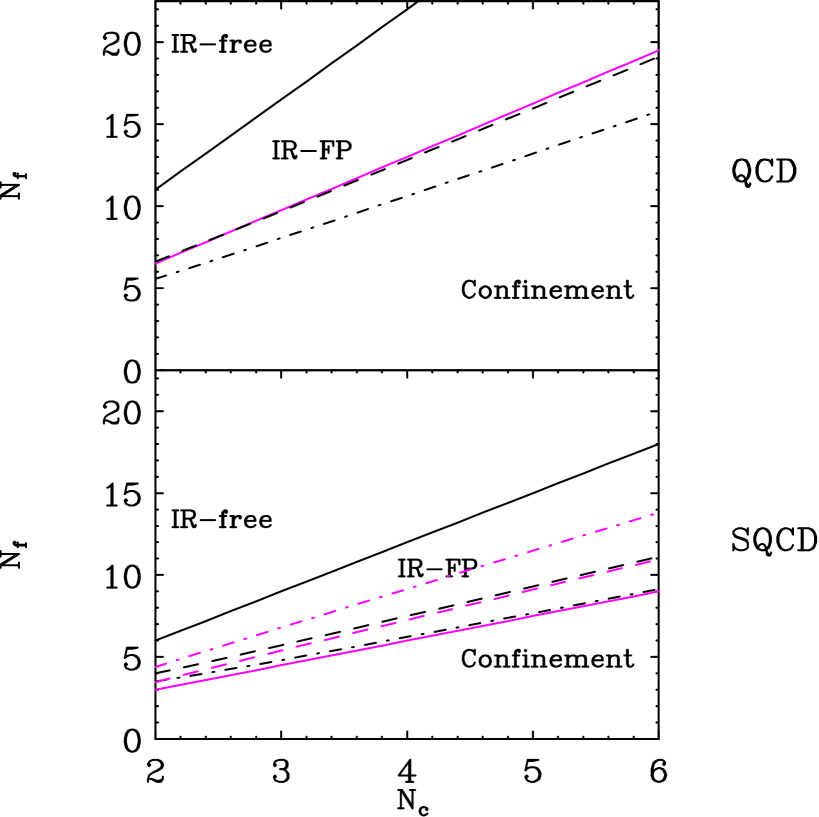
Figure 1: The conformal window in QCD (upper plot) and SQCD (lower plot) is shown in the $N_{f}\,\,-\,\,N_{c}$ plane. In both plots the $\beta_{0}=0$ line, separating the infrared free phase from the ultraviolet asymptotically free phase is drawn as a continuous black line. This line is the upper boundary of the conformal window. The lower boundary of the conformal window as implied by superconvergence is drawn in gray. In the SQCD case, this last line is also the line below which the dual theory becomes infrared free. In both plots, the (black) dashed line shows the lower boundary of the region where the 2-loop coupling has a causal analyticity structure. Below this line and above the dot-dash line there are complex Landau singularities. Below the dot-dash line there is a space-like Landau branch point. In the lower plot, we also show in gray the dual lines which describe the analyticity structure of the dual coupling constant.

The results are summarized in fig. 1 in the upper plot, where the lower boundary of the conformal window implied by superconvergence ($r=3.25$) is compared with the lower boundary of the region where the 2-loop coupling is causal according to (13), which is asymptotic at large $N_{c}$ to $r\simeq 3.17$. Clearly, the 2-loop coupling is causal in the entire conformal window. This conclusion holds, of course, also in the case where the lower boundary of the conformal window is somewhere above the critical value for superconvergence ($r=3.25$). This suggests that the fixed-point in QCD is always of perturbative origin.

The proximity of the two lines, the upper boundary of the superconvergence region ($r=3.25$) and the lower boundary of the 2-loop causality region ($r=3.17$) does not have any deep meaning. Presence of complex Landau singularities in the running coupling signals that the coupling becomes strong but it does not necessarily imply confinement – an example is provided by SQCD (Sec. 3).

Due to the closeness of the two lines one might worry that even within the conformal window the large distance physics cannot be reliably described by perturbation theory. However, we shall see in the next section that 3-loop corrections make the coupling causal in a wider range, and eventually perturbation theory does seem reliable down to the bottom of the conformal window.

2.2 How relevant is the criterion for causality at 2-loop?

It is natural to wonder whether the singularity structure of the coupling which is defined by the truncated 2-loop $\beta$ function is of any physical significance. Of course we do not doubt the assumption that the theory as a whole is causal. According to the common lore, the appearance of the non-physical Landau singularity in the perturbative coupling in real-world QCD is nothing more than a sign of the inapplicability of perturbation theory for describing the infrared region. Thus the presence of Landau singularity indicates the significance of non-perturbative corrections in the infrared. The interesting point is that close enough to the top of the conformal window, there may be a possibility to establish causality using only perturbation theory, as we explain below.

2.2.1 Causality beyond 2-loop – general discussion

In general, the analyticity structure of a coupling based on some higher order $\beta$ function,

$$\beta(x)=-\beta_{0}x^{2}\left[1+cx+c_{2}x^{2}+\cdots\right]$$ (16)

can be completely different from that of the 2-loop coupling (6). This is clearly so if Landau singularities are present: their location and nature generally depend on all the coefficients of the $\beta$ function and consequently on the renormalization scheme. This “instability” should be of no surprise since the weak coupling expansion breaks down completely when examining the singularities of the coupling.

As an example how the singularity structure changes and becomes more complex as higher order terms in the $\beta$ function are included, consider the 1-loop coupling, the 2-loop coupling and Padé improved 3-loop coupling, defined by

$$\beta_{\hbox{\tiny PA}}(x)=-\beta_{0}x^{2}\frac{1+[c-(c_{2}/c)]x}{1-(c_{2}/c)x},$$ (17)

which were all analyzed in [12]. The 1-loop coupling has a space-like Landau pole, the 2-loop coupling can have a causal structure or a pair of complex branch points or a space-like branch point. The Padé improved 3-loop coupling can be causal but it can also have both simple poles and branch points (the details appear in [12]).

While these examples show that there is no stability when going to higher orders if Landau singularities exist, they also indicate that if the 2-loop coupling is causal, causality may be preserved when higher order corrections are included. In fact, it is rather simple to explain why this kind of stability be expected in general. When the 2-loop coupling is causal it is bounded, and in many cases also small, for any complex $Q^{2}$. If so the usual perturbative justification holds: the next term in the $\beta$ function series which is proportional to a higher power of the coupling is small, and likewise higher order terms. In this situation higher-order terms are not expected to have much influence on $x(Q^{2})$. In other words, absence of Landau singularities can be consistently confirmed at the perturbative level, whereas presence of Landau singularities can only be confirmed or disproved in the full theory by non-perturbative methods.

The first step in establishing causality in perturbation theory is to examine the analyticity structure of the 2-loop coupling, as we did above. On one hand the 2-loop coupling has the advantage that it does not depend on the renormalization scheme. On the other hand it does not correspond directly to any observable and therefore it may not be causal. Thus, we are forced to examine higher order corrections (or renormalization schemes other than the ‘t Hooft scheme), and see whether the causality condition at 2-loop order is reasonable. The next step is therefore to choose a representative renormalization scheme, different from the ‘t Hooft scheme, and ask whether the 3-loop correction to the $\beta$ function has a significant effect on the infrared coupling. If the effect of the 3-loop correction is negligible, that is if the coupling is small enough such that

$$\left|\beta_{2}x^{2}(Q^{2})\right|\ll\left|\beta_{1}x(Q^{2})\right|$$ (18)

in the entire complex $Q^{2}$ plane, then we shall consider that causality is established at the perturbative level.

To be completely convinced, one might want to check also the magnitude of higher-order corrections corresponding to 4-loop order and beyond. However, it is important to remember in this respect, that if we go to high enough order ($n$), we will always obtain

$$\left|\beta_{n}x^{n}\right|>\left|\beta_{n-1}x^{n-1}\right|$$ (19)

due to the asymptotic nature of the $\beta$ function series, and thus it does not make sense to require that all the higher-order terms will be small. In the scenario described above, namely that the 2-loop coupling is already causal and small it seems reasonable to require that the 3-loop correction is small and stop there. Clearly, this scenario is just the simplest case to consider. It is possible that $x(Q^{2})$ at 2-loop is still not small enough so as to guarantee $|\beta_{2}x^{2}|\ll|\beta_{1}x|$, but $\beta_{2}$ is negative so $x(Q^{2})$ at 3-loop is much smaller, and then higher order corrections are negligible: $|\beta_{3}x^{3}|\ll|\beta_{2}x^{2}|$. Of course, in this case the results might depend on the renormalization scheme.

An encouraging observation with regards to the 2-loop analysis is that the condition for causality of the 3-loop coupling is quite modest once the 2-loop coupling is causal. We will show that the only further requirement is that the 3-loop $\beta$ function has a positive root corresponding to the infrared stable fixed-point.

It is most convenient for this demonstration to write the 3-loop $\beta$ function in the following form:

$$\beta(x)\equiv\frac{dx}{d\ln(Q^{2})}=-\beta_{2}x^{2}\left[f_{1}f_{2}-(f_{1}+f_{2})x+x^{2}\right]$$ (20)

where $f_{1}f_{2}=\beta_{0}/\beta_{2}$ and $f_{1}+f_{2}=-\beta_{1}/\beta_{2}$, thus:

$$f_{1} = \frac{1}{2\beta_{2}}\left(-\beta_{1}+\sqrt{\Delta}\right)$$ (21)

$$f_{2} = \frac{1}{2\beta_{2}}\left(-\beta_{1}-\sqrt{\Delta}\right)$$

with $\Delta=\beta_{1}^{2}-4\beta_{0}\beta_{2}$. Note that in all cases of interest, namely when there is a positive real zero to the 3-loop $\beta$ function, the infrared fixed-point is $x_{\hbox{\tiny IR}}\equiv f_{2}>0$, and $x_{\hbox{\tiny UV}}\equiv f_{1}$ is an ultraviolet fixed-point. The corresponding critical exponents are, for $x_{\hbox{\tiny IR}}$:

$$\gamma_{\hbox{\tiny IR}}^{3-loop}=\beta_{2}x_{\hbox{\tiny IR}}^{2}(x_{\hbox{\tiny UV}}-x_{\hbox{\tiny IR}})=x_{\hbox{\tiny IR}}^{2}\sqrt{\Delta}>0$$ (22)

and for $x_{\hbox{\tiny UV}}$:

$$\gamma_{\hbox{\tiny UV}}^{3-loop}=-\beta_{2}x_{\hbox{\tiny UV}}^{2}(x_{\hbox{\tiny UV}}-x_{\hbox{\tiny IR}})=-x_{\hbox{\tiny UV}}^{2}\sqrt{\Delta}<0.$$ (23)

It is useful to note that

$$\frac{1}{\gamma_{\hbox{\tiny UV}}^{3-loop}}+\frac{1}{\gamma_{\hbox{\tiny IR}}^{3-loop}}\,=\,\frac{1}{\gamma^{2-loop}}\,=\,-\frac{\beta_{1}}{\beta_{0}^{2}},$$ (24)

where we have used the definition of $f_{1,2}$. It then follows, assuming 2-loop causality (12), that

$$0<\gamma_{\hbox{\tiny IR}}^{3-loop}<\gamma^{2-loop}<1.$$ (25)

In order to examine causality at 3-loop we integrate (20) and obtain:

$$\ln(Q^{2}/\Lambda^{2})\,=\,\frac{1}{\beta_{0}x}+\frac{1}{\gamma_{\hbox{\tiny UV}}^{3-loop}}\ln\left[\frac{1}{x}-\frac{1}{x_{\hbox{\tiny UV}}}\right]+\frac{1}{\gamma_{\hbox{\tiny IR}}^{3-loop}}\ln\left[\frac{1}{x}-\frac{1}{x_{\hbox{\tiny IR}}}\right]$$ (26)

To find the causality condition, we study, as in the 2-loop case, the phase of the Landau singularity. We assume that the only singularities are such that $|x(Q^{2})|\longrightarrow\infty$, and expand (26) around these points in powers of $1/x$. The leading term in this expansion gives the location of the singularity. If $\beta_{2}<0$, then $x_{\hbox{\tiny UV}}$ is negative and the phase of the r.h.s. of (26) at the singularity is

$$\Phi\,=\,\pm\pi\,\frac{1}{\gamma_{\hbox{\tiny IR}}^{3-loop}},$$ (27)

while if $\beta_{2}>0$, $x_{\hbox{\tiny UV}}$ is positive and the phase is

$$\Phi\,=\,\pm\pi\,\left(\frac{1}{\gamma_{\hbox{\tiny UV}}^{3-loop}}+\frac{1}{\gamma_{\hbox{\tiny IR}}^{3-loop}}\right)\,=\pm\,\pi\,\frac{1}{\gamma^{2-loop}}.$$ (28)

Using (25) we find that in both cases $|\Phi|>\pi$ and it follows that the 3-loop coupling is causal.

We showed that if the 2-loop coupling is causal, the 3-loop coupling is also causal, provided it has an infrared fixed-point. It is not clear whether such a conclusion can be extended to higher orders. It may be however interesting to note that we already know from the analysis of [12] another example where similar conclusions hold: this is the Padé improved 3-loop $\beta$ function, defined by (17). Contrary to the above examples, this $\beta$ function is not truncated at some finite order, and thus it could be expected a priori to behave differently. According to [12] the causality condition for the Padé-improved 3-loop coupling is $c<-\beta_{0}$ and $c_{2}<c^{2}$. The first condition is the same as the condition for the causality of the 2-loop coupling. In fact, the critical exponent of this coupling is equal to that of the 2-loop coupling, and thus the condition is $0<\gamma^{\hbox{\tiny PA}}=\gamma^{2-loop}<1$. The second condition is just the condition to have a positive infrared fixed-point.

We comment that the inverse statement does not hold: the 3-loop coupling can be causal even if the 2-loop coupling is not. If $\beta_{2}$ is negative and large enough, the 3-loop coupling is causal independently of the sign of $\beta_{1}$.

Coming to analyze the conditions for causality or the stability of the causal solution with respect to higher order corrections (such as (18)), we should, in general solve the renormalization group equation at each order to obtain $x(Q^{2})$ in the entire $Q^{2}$ plane, as was done in [12] for the 2-loop and the Padé improved 3-loop couplings. However, we shall demonstrate below that it is in fact enough to examine the effect of higher orders on the infrared limit of the space-like coupling $x_{\hbox{\tiny FP}}\equiv x(0)$, unless the coefficients of the $\beta$ function are extremely close to the condition where causality is lost. In most cases when $x(Q^{2})$ is causal, $|x(Q^{2})|\mathrel{\mathchoice{\vbox{\offinterlineskip\halign{$\m@th\displaystyle\hfil#\hfil$\cr<\crcr\sim\crcr} }}{\vbox{\offinterlineskip\halign{$\m@th\textstyle\hfil#\hfil$\cr<\crcr\sim\crcr} }}{\vbox{\offinterlineskip\halign{$\m@th\scriptstyle\hfil#\hfil$\cr<\crcr\sim\crcr} }}{\vbox{\offinterlineskip\halign{$\m@th\scriptscriptstyle\hfil#\hfil$\cr<\crcr\sim\crcr} }}}x(0)$ in the entire $Q^{2}$ plane. Of course, when causality is lost $x(Q^{2})$ diverges at some point while $x(0)$ is finite, and thus close to the boundary of the causality region $x(0)$ is not indicative at all. The point is that the region where the maximum value of $|x(Q^{2})|$ is much larger than $x(0)$ is quite narrow. To demonstrate this, consider again the example of 2-loop coupling in $N_{c}=3$ QCD. According to (13) this coupling is causal so long as $N_{f}\mathrel{\mathchoice{\vbox{\offinterlineskip\halign{$\m@th\displaystyle\hfil#\hfil$\cr>\crcr\sim\crcr} }}{\vbox{\offinterlineskip\halign{$\m@th\textstyle\hfil#\hfil$\cr>\crcr\sim\crcr} }}{\vbox{\offinterlineskip\halign{$\m@th\scriptstyle\hfil#\hfil$\cr>\crcr\sim\crcr} }}{\vbox{\offinterlineskip\halign{$\m@th\scriptscriptstyle\hfil#\hfil$\cr>\crcr\sim\crcr} }}}9.683$. At the point where causality is lost, $|x(Q^{2})|$ reaches infinity on the first sheet (on the time-like axis), while the space-like coupling has its maximum at $x(0)\simeq 0.88$ which is not so large. However, if we move slightly above the causality boundary, the maximal value of $|x(Q^{2})|$ in the entire $Q^{2}$ plane becomes of the order of $x(0)$. We show this phenomenon in fig. 2 where we plot the region in the complex coupling plane, into which the entire complex $Q^{2}$ plane is mapped. The contour itself corresponds to the cut along the time-like axis ($Q^{2}<0$) and it was computed using the Lambert W function solution, as explained in [12, 11]. As shown in the plot, for $N_{f}=9.7$, i.e. very close to the point where causality is lost, the maximal value of $|x(Q^{2})|$ on the time-like axis is still significantly larger than $x(0)$. One clearly identifies here the effects of the singularities that are present on the second sheet. On the other hand, already at $N_{f}=10$, the maximal value of $|x(Q^{2})|$ on the time-like axis is of the order of $x(0)$.

We found that the condition for the 2-loop coupling to have a causal analyticity structure is $0\leq\gamma^{2-loop}<1$, where $\gamma^{2-loop}=0$ corresponds to a free theory, the limit obtained at the top of the conformal window, and $\gamma^{2-loop}=1$ corresponds to the point where Landau singularities first appear. At 2-loop order the condition $0\leq\gamma^{2-loop}<1$ is both a sufficient and a necessary condition. It is interesting to see how this generalizes to higher orders. When the $\beta$ function has more than one zero, we should specify at which of them $\gamma$ is defined. The only root that is relevant in the asymptotically free phase is the smallest positive zero, the physical infrared stable fixed-point, and we always refer to this one.

The 3-loop analysis shows that $0\leq\gamma^{3-loop}<1$ is a necessary condition but not a sufficient one. An example where the 3-loop coupling is not causal although the above condition is obeyed can be constructed starting with a non-causal 2-loop $\beta$ function with $\beta_{1}<0$ and adding a 3-loop term with $\beta_{2}$ positive but small enough such that a positive zero for the 3-loop $\beta$ function exists. It then follows from eq. (28) that the 3-loop coupling is not causal although $\gamma^{3-loop}$ can still obey the above condition. We stress that this example is not representative since usually, as we shall see, $\beta_{2}<0$ and then the condition $0\leq\gamma<1$ is both necessary and sufficient also at the 3-loop order.

In fact the condition $0\leq\gamma<1$ is always necessary for a causal analyticity structure. The condition $\gamma\geq 0$ is simply the one to have an infrared stable fixed-point. To show that also $\gamma<1$ is necessary we use the following observation: a causal structure implies that there is a well defined mapping $x(Q^{2})$ from the entire complex $Q^{2}$ (the first sheet) into a compact domain in the complex coupling plane, such that for large enough $|Q^{2}|$ the coupling flows to the trivial fixed-point, as implied by asymptotic freedom. As we saw in the example of fig. 2 (these features as completely general) the space-like axis is mapped to real positive values in the range $[0,x_{\hbox{\tiny FP}}]$ and the time-like axis is mapped to the boundary of this domain in the complex coupling plane. It follows from the definition of $\gamma$ in (10) that the coupling approaches the fixed-point according to

$$x=x_{\hbox{\tiny FP}}-\left(\frac{Q^{2}}{\Lambda_{\hbox{\tiny eff}}^{2}}\right)^{\gamma},$$ (29)

where $\Lambda_{\hbox{\tiny eff}}$ is an observable-dependent QCD scale. If $\gamma>1$, there is a phase $\Phi=\pi/\gamma$ in the complex $Q^{2}$ plane ($Q^{2}=Q_{0}^{2}\exp(i\Phi)$) such that in the limit $Q^{2}_{0}\longrightarrow 0$ the rays $\pm\Phi$ are mapped by (29) to positive real values of the coupling larger than the fixed-point value ($x=x_{\hbox{\tiny FP}}^{+}$). On the other hand a straightforward analysis of the $\beta$ function shows that values of the coupling $x>x_{\hbox{\tiny FP}}$ either belong to the domain of attraction of some non-trivial ultraviolet fixed-point or flow to an ultraviolet Landau singularity. The conclusion is that there is no singularity free mapping that obeys the asymptotic freedom condition stated above. In particular, if two different ultraviolet fixed-points are allowed for different values of $Q^{2}$ it implies the existence of a separatrix, discriminating between the values of $Q^{2}$ that flow to each of the ultraviolet fixed-points, i.e. there are singularities in the first sheet of the complex $Q^{2}$ plane. We stress that the arguments why $0\leq\gamma<1$ is a necessary condition for a causal analyticity structure are completely general: they are not based on perturbation theory.

2.2.2 Causality at higher orders in QCD

We would like to examine whether causality can be established in perturbation theory in the specific case of the conformal window in QCD. Close to the top of the conformal window, causality is established at the 2-loop level. The infrared coupling is small and thus the 3-loop term is negligible and condition (18) for stability of the perturbative analysis is obeyed. This is no longer true at the bottom of the window.

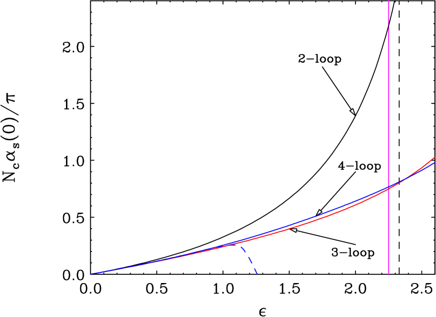
Figure 3: The infrared limit of the 2-loop coupling and the 3-loop and 4-loop $\overline{\hbox{MS}}\,$ couplings in large $N_{c}$ QCD as a function of $\epsilon\equiv(11/2)-(N_{f}/N_{c})$. The dashed line corresponds to the 20th order Taylor expansion in $\epsilon$ of the 4-loop coupling. The continuous vertical line represents the bottom of the conformal window implied by superconvergence and the dashed vertical line shows the 2-loop causality boundary.

We start the discussion in the $\overline{\hbox{MS}}\,$ scheme, which has the advantage that the 4-loop coefficient in the $\beta$ function is known [24, 25]. We shall refer to physical effective charges later. The fixed-point value of the coupling, calculated as an explicit solution of the equation $\beta(x)=0$ in the large $N_{c}$ limit at 2-loop and then in the $\overline{\hbox{MS}}\,$ scheme at 3-loop and 4-loop orders is shown in fig. 3 as a function of the distance from the top of the conformal window,

$$\epsilon\equiv\frac{11}{2}-r=\frac{11}{2}-\frac{N_{f}}{N_{c}}.$$ (30)

The 2-loop coupling reaches relatively large values towards the bottom of the conformal window, but then the 3-loop and 4-loop couplings take significantly lower values, and in addition they are very close to each other. These results can be understood knowing the negative sign of the 3-loop coefficient $\beta_{2}$ and the magnitude of successive terms in the $\overline{\hbox{MS}}\,$ scheme, shown in fig. 4. In the latter, the coupling is evaluated at the fixed-point according to the zero of the 3-loop $\beta$ function. It is clear from the plot that the condition for stability of the 2-loop result (18) does not hold in the lower part of the conformal window. It certainly does not hold for $r\mathrel{\mathchoice{\vbox{\offinterlineskip\halign{$\m@th\displaystyle\hfil#\hfil$\cr<\crcr\sim\crcr} }}{\vbox{\offinterlineskip\halign{$\m@th\textstyle\hfil#\hfil$\cr<\crcr\sim\crcr} }}{\vbox{\offinterlineskip\halign{$\m@th\scriptstyle\hfil#\hfil$\cr<\crcr\sim\crcr} }}{\vbox{\offinterlineskip\halign{$\m@th\scriptscriptstyle\hfil#\hfil$\cr<\crcr\sim\crcr} }}}4$, corresponding to $N_{f}\mathrel{\mathchoice{\vbox{\offinterlineskip\halign{$\m@th\displaystyle\hfil#\hfil$\cr<\crcr\sim\crcr} }}{\vbox{\offinterlineskip\halign{$\m@th\textstyle\hfil#\hfil$\cr<\crcr\sim\crcr} }}{\vbox{\offinterlineskip\halign{$\m@th\scriptstyle\hfil#\hfil$\cr<\crcr\sim\crcr} }}{\vbox{\offinterlineskip\halign{$\m@th\scriptscriptstyle\hfil#\hfil$\cr<\crcr\sim\crcr} }}}12$ since there the 3-loop term is comparable to the 2-loop term. Thus we are forced to examine causality at higher orders.

Since the 3-loop coefficient in $\overline{\hbox{MS}}\,$ is negative for the relevant $N_{f}/N_{c}$ values, the 3-loop $\beta$ function has a positive real fixed-point, and according to the general discussion in the previous section, 3-loop causality is implied within the region where the 2-loop coupling is causal. Now, in order to trust the 3-loop causality, it is required that the 4-loop term will be small enough. Indeed, as shown in fig. 4 the 4-loop term in the $\overline{\hbox{MS}}\,$ scheme remains small in the entire conformal window. The effect of the 4-loop term on the fixed-point value is shown in fig. 3. Clearly, this is a negligible effect, and thus perturbative stability is realized at the 3-loop level. It would be better to check the effect of the 4-loop term on $x(Q^{2})$ in the entire $Q^{2}$ plane, but based on the experience with the 2-loop coupling we expect that in general the space-like fixed-point value is indicative of the magnitude of $x(Q^{2})$ in the entire complex $Q^{2}$ plane.

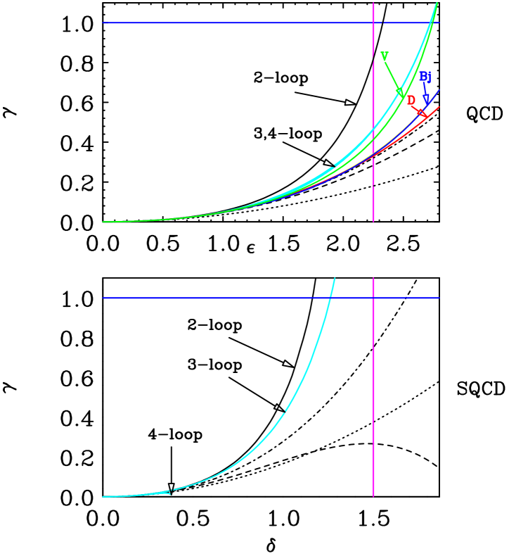
Figure 5: The critical exponent $\gamma$ in large $N_{c}$ QCD (SQCD) is shown in the upper (lower) plot as a function of $\epsilon=(11/2)-(N_{f}/N_{c})$ ($\delta=3-(N_{f}/N_{c})$), according to an explicit calculation from the truncated 2-loop $\beta$ function and the 3-loop and 4-loop $\beta$ functions (the loop order is indicated by the arrows) in the $\overline{\hbox{MS}}\,$ (DRED) renormalization scheme as well as according to the three available partial sums in the Banks-Zaks expansion: leading order – dotted line, next-to-leading order – dot-dashed line, and next-to-next-to-leading order – dashed line. In the QCD plot we show also the explicit calculation of $\gamma$ at the 3-loop order in various physical renormalization schemes defined from the vacuum polarization D-function (D), the polarized and non-polarized Bjorken sum-rules (Bj) and the heavy quark effective potential (V). The vertical arrow in the SQCD plot shows the point where the positive real zero of the 4-loop $\beta$ function disappears. The vertical line is the bottom of the conformal window according to superconvergence and the horizontal $\gamma=1$ line is the necessary upper bound of $\gamma$ for a causal analyticity structure.

Next we consider the value of the critical exponent as a function of the distance from the top of the window. The results of an explicit calculation of $\gamma$, in the large $N_{c}$ limit, from the 2-loop, 3-loop and 4-loop $\beta$ functions in $\overline{\hbox{MS}}\,$ are shown in fig. 5 in the upper plot. In agreement with our previous discussion the condition $0<\gamma^{3-loop}<\gamma^{2-loop}<1$ is obeyed in the entire conformal window. The points where the 2-loop and 3-loop couplings cease to be causal can be identified in this figure as the points where $\gamma=1$. Since the 4-loop term is small, $\gamma^{4-loop}\simeq\gamma^{3-loop}$ within the resolution of this plot, and so the perturbative stability which characterises the coupling exists also for the critical exponent.

We stress that the results described above are not special to the large $N_{c}$ limit. In particular fig. 3 through 5 are qualitatively the same for any $N_{c}$.

The above investigation shows that the $\overline{\hbox{MS}}\,$ coupling is causal at the 3-loop level and, given the smallness of the 4-loop term, presumably also at the 4-loop level in the entire conformal window. However, this coupling does not correspond directly to any observable quantity. It is important to check whether similar conclusions apply in physical schemes.

A relevant analysis has been performed in [11]. Fig. 1 in [11] compares the $N_{f}$ dependence of $c_{2}\equiv\beta_{2}/\beta_{0}$ for various physical effective charges. The observation that $c_{2}$ for different effective charges are numerically close and that they share the same $N_{f}$ dependence indicates that certain properties of the coupling may be generic in spite of scheme dependence. In particular we note that $c_{2}$ is negative in the entire conformal window not only in $\overline{\hbox{MS}}\,$, but also for all the physical effective charges considered. We conclude that there is a fixed-point at the 3-loop order in all these physical schemes and, according to the general discussion above, 3-loop causality follows. Unfortunately, 4-loop coefficients in physical renormalization schemes are not known yet. Consequently, the stability of the 3-loop causal coupling with respect to higher loop corrections cannot be studied for physical effective charges like we did in the $\overline{\hbox{MS}}\,$ scheme. However an alternative is provided by the Banks-Zaks expansion, which can be calculated in physical schemes up to next-to-next-to-leading order term [14, 15, 11]. This will be discussed further in Sec. 4.

We comment that the perturbative coupling at the 3-loop order can have a causal analyticity structure even somewhat below the bottom of the conformal window, i.e. in the upper part of the confining phase. In this respect, different couplings may behave differently. We recall that for $N_{c}=3$ the ‘t Hooft coupling, defined by the truncated 2-loop $\beta$ function, is causal down to $N_{f}\simeq 9.68$, quite close to the bottom of the conformal window $N_{f}\simeq 9.75$. This can be compared with the $\overline{\hbox{MS}}\,$ scheme where 3-loop causality is lost at $N_{f}\simeq 8.5$ and to physical renormalization schemes in which the causality domain is even wider. Based on the results of [11] and the above type of analysis we find that for the effective charge defined by the vacuum polarization D-function and the ones associated with the polarized and non-polarized Bjorken sum-rules 3-loop causality is lost at $N_{f}\simeq 7.2$ while for the effective charge defined from the heavy quark potential 3-loop causality is lost at $N_{f}\simeq 8.4$.

Finally we consider the calculation of the critical exponent using physical renormalization schemes. As long as the fixed point is perturbative, it is natural to expect that $\gamma$ could be calculated with a reasonable accuracy starting with the truncated $\beta$ function in various renormalization schemes. Since $\gamma$ is a universal quantity the results should agree. The results of an explicit calculation of $\gamma$ in several physical schemes at the 3-loop order are presented in fig. 5 together with the results in $\overline{\hbox{MS}}\,$. The schemes we use include the vacuum polarization D-function, the polarized and non-polarized Bjorken sum-rules (the latter two curves overlap) and the heavy quark effective potential. The results in the different schemes agree very well close to the top of the window. The spread increases to about $\pm 15\%$ towards the bottom of the window and is interpreted as an artifact of using a truncated perturbative expansion. We shall come back to discuss the accuracy to which $\gamma$ can be calculated in sec. 4.2.1 in the framework of the Banks-Zaks expansion (see table 5 there).

3 The conformal window in SQCD

The $\beta$ function in SQCD is given by

$$\beta(x)\,\equiv\,\frac{dx}{d\ln(Q^{2})}\,=\,-(B_{0}x^{2}+B_{1}x^{3}+\cdots)\,=\,-B_{0}x^{2}\,(1+C_{1}x+\cdots)$$ (31)

where $x=\alpha/\pi=g^{2}/(4\pi^{2})$,

$$B_{0}=\frac{1}{4}\left(3N_{c}-N_{f}\right),$$ (32)

and

$$C_{1}\equiv\frac{B_{1}}{B_{0}}=\frac{1}{2}N_{c}-\frac{N_{f}}{3N_{c}-N_{f}}\frac{N_{c}^{2}-1}{2N_{c}},$$ (33)

where the coefficients where calculated in [28]. Above the line $R\equiv N_{f}/N_{c}=3$ the theory is infrared free, while below this line it is asymptotically free in the ultraviolet. For $R$ just below $3$, $B_{0}$ is small and positive and $B_{1}$ is negative, leading to an infrared fixed-point at a small $x_{\hbox{\tiny FP}}\simeq-B_{0}/B_{1}=-1/C_{1}$, making the theory weakly coupled at all scales. As $N_{f}$ (and thus $R$) is decreased, the infrared coupling increases. According to Seiberg [16], the infrared fixed-point persists even down to such low $N_{f}$ that the original degrees of freedom are strongly coupled and then a dual theory which is based on another gauge group with $N_{c}^{d}=N_{f}-N_{c}$ colors is appropriate to describe the infrared limit ($d$ stands for a dual variable). Seiberg’s conjecture can only be understood if the fixed-point is of non-perturbative origin, at least in the lower part of the conformal window. This is contrary to our previous observation concerning the perturbative origin of the fixed-point in the non-supersymmetric case. Thus we would like to check that indeed a definite difference exists between the conformal window in QCD, which is perturbative and the one in SQCD which is not. This is done here by considering the analyticity structure of the coupling constant and in the next section, by comparing the Banks-Zaks expansion in SQCD to that in QCD. We shall indeed see that already at the perturbative level SQCD is more strongly coupled than QCD in the lower part of the conformal window. The fact that the strong coupling nature of SQCD at the lower part of the window is manifested in perturbation theory is not obvious a priori; strong infrared effects could have been induced instead by terms invisible to perturbation theory.

Duality [16] provides an intuitive description of the conformal window in SQCD, which is absent in QCD. The lower boundary of the conformal window in SQCD is naturally identified as the $R\equiv N_{f}/N_{c}$ ratio at which the dual theory undergoes a phase transition from the asymptotically free phase (inside the window) to the infrared free phase (below the window). The 1-loop $\beta$ function coefficient in the dual theory can be obtained by substituting $N_{f}-N_{c}$ for $N_{c}$ in (32):

$$B_{0}^{d}=\frac{1}{4}\left(2N_{f}-3N_{c}\right).$$ (34)

Thus, the conformal window is $3/2<R<3$, as shown in the lower plot of fig. 1. The original theory is weakly coupled, and therefore provides a natural physical description, for $R$ just below the line $R=3$, while the dual theory is weakly coupled just above the line $R=3/2$.

An important consistency check for both duality and the superconvergence criterion for confinement is that the lower boundary of the conformal window in both approaches coincides [19]. The observation of [19] is the following: in SQCD the anomalous dimension of the gluon propagator in the Landau gauge is

$$\gamma_{00}^{\rm SQCD}=-\frac{1}{4}\left(\frac{3}{2}N_{c}-N_{f}\right),$$ (35)

which is just proportional to the first coefficient of the $\beta$ function $B_{0}^{d}$ in the dual theory. As a result, $\gamma_{00}^{\rm SQCD}$ becomes negative, implying superconvergence and therefore confinement for the original theory, as $R$ becomes smaller than $3/2$, i.e. exactly where the dual theory becomes infrared free ($B_{0}^{d}$ in (34) changes sign).

3.1 The analyticity structure of the SQCD coupling

The purpose of this section is to analyze the singularity structure of the perturbative SQCD coupling, in parallel with the analysis of the QCD coupling in Sec. 2, and in particular to find when it is consistent with causality.

The first step is to analyse the 2-loop coupling. The 2-loop causality condition $C_{1}<-B_{0}$ translates, using eqs. (32), and (33), to the following condition for $R$:

$$R^{2}+\left[\frac{2}{N_{c}^{2}}-10\right]R+15<0.$$ (36)

Similarly to the non-supersymmetric case (see eq. (13)), the condition (36) leads to an approximately $N_{c}$ independent critical value for $R$ for any possible value of $N_{c}$ (since $N_{c}^{2}\gg 2/10$), namely the 2-loop coupling is causal as long as

$$R>5-\sqrt{10}\simeq 1.8377.$$ (37)

The crucial observation is that the line (37) that limits from below the region where the 2-loop coupling is causal, is within the conformal window which has its lower boundary at $R=3/2$. This is shown in the lower plot of fig. 1. The situation encountered here is contrary to the one in non-supersymmetric QCD, where the 2-loop perturbative coupling is causal in the entire conformal window. This observation fits the general expectation based on duality, that the fixed-point in SQCD is non-perturbative in the lower part of the conformal window.

In addition we ask when does the 2-loop coupling develop a space-like Landau singularity. The condition $C_{1}>0$ translates (using (33)) to the following:

$$R<\frac{3}{2-(1/N_{c}^{2})},$$ (38)

which is asymptotic in the large $N_{c}$ limit to the lower boundary of the conformal window, $R=3/2$.

Note that in the supersymmetric case, it is natural to use the NSVZ form [28, 29] of the $\beta$ function, and thus one may wonder if our results concerning the analyticity structure of the coupling may vary when using the $\beta$ function in this form rather than the truncated 2-loop one. In the Appendix we show that both the condition for a causal coupling and the condition for a space-like Landau singularity are exactly the same in the two cases, if in the NSVZ form one uses the leading order approximation for the matter field anomalous dimension.

The next step in the analysis of the perturbative coupling causality, as in the QCD case, should be to examine the effect of higher order terms in the perturbative $\beta$ function. We choose to work in the DRED renormalization scheme [27], assuming that our conclusions will not depend on this choice.

The explicit solutions of $\beta(x)=0$ for $N_{c}x(0)$ in the large $N_{c}$ limit are shown in fig. 6 as a function of the distance from the top of the conformal window,

$$\delta\equiv 3-R=3-\frac{N_{f}}{N_{c}}.$$ (39)

The 2-loop solution is infinite at the bottom of the window (see (38)). Already here we encounter a situation different from QCD, namely stronger coupling. Since the 3-loop coefficient is negative, the 3-loop solution is smaller. The latter is finite down to the bottom of the window, but it is still rather large. The fixed-point at 4-loop order exists only up to $\delta\simeq 0.4$ (near the 4-loop arrow in the figure). Beyond this point there is no positive real solution to the equation $\beta(x)=0$. The reason is that the 4-loop term in SQCD is positive (like in QCD) and large (contrary to QCD) as can be learned from fig. 7. This figure shows the relative magnitude of the four leading terms in the large $N_{c}$ SQCD $\beta$ function. The coupling in fig. 7 is evaluated as the zero of the 3-loop $\beta$ function.

In the lower plot of fig. 5 we show the value of the critical exponent as a function of $\delta$ according to the 2-loop, 3-loop and 4-loop order large $N_{c}$ DRED $\beta$ function. The necessary condition for a causal structure $\gamma=1$ is reached by both the 2-loop order, which was discussed above, and 3-loop order solutions for $\gamma$ well within the conformal window. The 4-loop result for $\gamma$ exists of course only up to $\delta\simeq 0.4$ where a positive fixed-point exists.

Examining fig. 5 through 7 we can determine where causality can be established in SQCD at the perturbative level. In the upper part of the conformal window the 3-loop term is small with respect to the 2-loop one, so one can trust 2-loop causality. As $R$ is decreased the 3-loop term becomes comparable to the 2-loop term and then one has to consider causality at 3-loop order. The negative sign of $\beta_{2}$ guarantees that the 3-loop coupling is causal at least as long as the 2-loop coupling is. But since the 4-loop term is very large, the perturbative argumentation fails. Thus in SQCD, it is possible to establish causality in perturbation theory only in the upper part of the conformal window. To be specific, two alternative criterions can be considered: the first is to require that the 3-loop term will be smaller than the 2-loop term. The two become equal around $R\simeq 1.9$, i.e. just above the 2-loop causality boundary. The second is even more restrictive, namely to require that also the 4-loop term is small, or that the 4-loop $\beta$ function will have a positive real root. This is realized only above $R\simeq 2.6$.

Maybe the most interesting observation in fig. 7 is the fact that the 4-loop term in the SQCD $\beta$ function is larger than the leading terms already very close to the top of the conformal window. This may be related to the asymptotic nature of the $\beta$ function series. The asymptotic behavior is another aspect in which the SQCD $\beta$ function is presumably different from the QCD one, a point which certainly deserves further study.

3.2 Reduction of Couplings in the magnetic theory

In the previous section we studied the singularity structure of the 2-loop coupling in the electric theory. Our aim here is to perform a parallel analysis in its dual, the magnetic theory. This is, however, not straightforward since the magnetic theory has two couplings, rather than one. The running of the gauge coupling is affected by the Yukawa interaction of the chiral quark superfields with the mesons, which is described by the superpotential (5). This gives rise to coupled renormalization group equations of the form

$$\beta^{d}_{x}(x,\lambda)\equiv\frac{dx}{d\ln(Q^{2})} = -B_{0}^{d}\,x^{2}-B_{1}^{d}\,x^{3}-B_{1,\lambda}^{d}x^{2}\lambda+\cdots$$ (40)

$$\beta^{d}_{\lambda}(x,\lambda)\equiv\frac{d\lambda}{d\ln(Q^{2})} = C_{\lambda}^{d}\,x\,\lambda+C_{\lambda\lambda}^{d}\,\lambda^{2}+\cdots$$

with

$$B_{0}^{d} = \frac{1}{4}\left(2N_{f}-3N_{c}\right)$$ (41)

$$B_{1}^{d} = \frac{1}{8}\left(N_{f}-N_{c}\right)\left(2N_{f}-3N_{c}\right)-\frac{N_{f}}{8}\,\frac{\left(N_{f}-N_{c}\right)^{2}-1}{N_{f}-N_{c}}$$

$$B_{1,\lambda}^{d} = \frac{1}{4}N_{f}^{2}$$

$$C_{\lambda}^{d} = -\frac{1}{2}\frac{\left(N_{f}-N_{c}\right)^{2}-1}{N_{f}-N_{c}}$$

$$C_{\lambda\lambda}^{d} = \frac{1}{2}\left(3N_{f}-N_{c}\right)$$

where $B_{0}^{d}$ and $B_{1}^{d}$ can be obtained by substituting $N_{c}\longrightarrow N_{f}-N_{c}$ in $B_{0}$ and $B_{1}$, and the other coefficients where calculated in [30]. Note that in (41) we use $N_{c}$ to denote the number of colors in the original (electric) theory, and thus the dual theory has an $SU(N_{f}-N_{c})$ gauge symmetry. This is contrary to the notation used in [30] that corresponds to an $SU(N_{c})$ gauge group in the magnetic theory. In addition, note that in [30] there is a typo in eq. (64), where a factor of two is missing in the second term in the second equation. The correct factor can be easily obtained by using eqs. (55), (62) and (63) there. Our coefficients do agree with those in [31].

In order to study the analyticity structure of the coupling in the magnetic theory one should, in principle, integrate the coupled renormalization-group equation (40). This is, however, rather complicated, and so we choose a simpler approach (which remains to be further justified) based on the notion of Reduction of Couplings.

It was recently shown by Oehme [31] that there is a unique reduction of the coupled renormalization-group equation (40) to a single-coupling equation such that the superpotential does not vanish, which is essential for duality. Ref. [31] describes in detail how to apply the general method of Reduction of Couplings to this problem. We shall use here only the leading order relation between $\lambda$ and $x$. To obtain the relation between the couplings one assumes

$$\lambda(x)=f(N_{c},N_{f})\,x+{\cal O}(x^{2})$$ (42)

and imposes the consistency condition,

$$\beta^{d}_{\lambda}\left(x,\lambda(x)\right)\,=\,\frac{d\lambda(x)}{dx}\,\beta^{d}_{x}\left(x,\lambda(x)\right).$$ (43)

Using (40), the condition (43) leads, at leading order, to:

$$f(N_{c},N_{f})\left[C_{\lambda\lambda}^{d}\,f(N_{c},N_{f})+C_{\lambda}^{d}+B_{0}^{d}\right]\,=\,0$$ (44)

and for a non-vanishing superpotential, the results is

$$f(N_{c},N_{f})\,=\,\frac{-B_{0}^{d}-C_{\lambda}^{d}}{C_{\lambda\lambda}^{d}}\,=\,\frac{N_{c}N_{f}-N_{c}^{2}-2}{2\left(N_{f}-N_{c}\right)\left(3N_{f}-N_{c}\right)}.$$ (45)

Note that $f(N_{c},N_{f})$ is positive in the entire conformal window.

With the result (45) at hand we can substitute the $\lambda$ term for $f(N_{c},N_{f})\,x$ in the equation of $\beta^{d}_{x}(x,\lambda)$ and obtain a single-coupling renormalization-group equation which is valid up to 2-loop order:

$$\beta^{d}_{x}(x,\lambda(x))\equiv\frac{dx}{d\ln(Q^{2})}=-B_{0}^{d}\,x^{2}-\tilde{B}_{1}^{d}\,x^{3}+\cdots$$ (46)

where

$$\tilde{B}_{1}^{d}=B_{1}^{d}+B_{1,\lambda}^{d}\,f(N_{c},N_{f}).$$ (47)

Next, we would like to analyze the analyticity structure of the coupling in the dual theory, using the reduced $\beta$ function (46). Let us calculate first the condition for the dual 2-loop coupling to have a causal analyticity structure (the analog of (37) in the original theory). The causality condition, $\tilde{B}_{1}^{d}/B_{0}^{d}<-B_{0}^{d}$, yields

$$18R^{3}-64R^{2}+\left[65+\frac{2}{N_{c}^{2}}\right]R-15<0$$ (48)

which again leads to an approximately $N_{c}$ independent critical value for $R$ for any possible value of $N_{c}$ (since $N_{c}^{2}\gg 2/65$), namely the 2-loop coupling in the dual theory is causal as long as

$$R\mathrel{\mathchoice{\vbox{\offinterlineskip\halign{$\m@th\displaystyle\hfil#\hfil$\cr<\crcr\sim\crcr} }}{\vbox{\offinterlineskip\halign{$\m@th\textstyle\hfil#\hfil$\cr<\crcr\sim\crcr} }}{\vbox{\offinterlineskip\halign{$\m@th\scriptstyle\hfil#\hfil$\cr<\crcr\sim\crcr} }}{\vbox{\offinterlineskip\halign{$\m@th\scriptscriptstyle\hfil#\hfil$\cr<\crcr\sim\crcr} }}}1.8357.$$ (49)

As with the original theory, the 2-loop causality region of the dual perturbative coupling does not cover the far-end of the window. Note (fig. 1) that the regions of a causal 2-loop coupling in the two dual descriptions, (37) and (49) do not overlap. This fits the intuition on which duality is based, i.e. that when one theory is weakly coupled its dual is necessarily strongly coupled. Since we assume that within the window a consistent perturbation theory implies small non-perturbative effects, an overlap would lead to contradiction: it would suggest that two different weakly coupled theories can describe the same infrared physics.

In fig. 1 the 2-loop causality boundaries in the two theories are very close. However, if one adopts a conservative attitude that perturbation theory actually breaks down above the 2-loop causality boundary (taking into account the large 4-loop correction) the perturbative regions of the two theories will be more separated.

One can also find the condition to have no space-like Landau singularity in the 2-loop reduced coupling. The requirement $\tilde{B}_{1}^{d}<0$ translates into the condition

$$3R^{3}-12R^{2}+\left[13+\frac{1}{N_{c}^{2}}\right]R-3<0,$$ (50)

which yields (for $N_{c}^{2}\gg 1/13$),

$$R\mathrel{\mathchoice{\vbox{\offinterlineskip\halign{$\m@th\displaystyle\hfil#\hfil$\cr<\crcr\sim\crcr} }}{\vbox{\offinterlineskip\halign{$\m@th\textstyle\hfil#\hfil$\cr<\crcr\sim\crcr} }}{\vbox{\offinterlineskip\halign{$\m@th\scriptstyle\hfil#\hfil$\cr<\crcr\sim\crcr} }}{\vbox{\offinterlineskip\halign{$\m@th\scriptscriptstyle\hfil#\hfil$\cr<\crcr\sim\crcr} }}}2.314.$$ (51)

Note that this line is below the top of the window, and thus in the upper part of the conformal window the dual coupling has a space-like singularity.

3.3 Summary

To conclude this part, let us summarize the differences between QCD and SQCD with respect to the analyticity structure of the coupling in comparison with the boundaries of the conformal window (fig. 1).

In QCD, the region of a causal 2-loop coupling covers the entire conformal window (supposing the lower boundary is determined by superconvergence: $r=3.25$). As $r$ is reduced further (below $r\simeq 3.17$), the 2-loop coupling develops a couple of Landau branch points at complex $Q^{2}$ values. At even lower $r$, below $r\simeq 2.62$, a Landau branch point appears on the space-like axis.

Studying higher loop effects we showed that the 3-loop term is important in the lower part of the conformal window, and so the 3-loop coupling should be referred to as a zeroth order approximation in the infrared. The next observation is that the 3-loop coefficient is negative in the conformal window both in $\overline{\hbox{MS}}\,$ and in all the physical effective charges for which the 3-loop coefficient has been computed. This means that the 3-loop coupling is causal at least where the 2-loop coupling is, i.e. in the entire conformal window, and in many cases, depending on $\beta_{2}$, also somewhat below this region into the upper part of the confining phase. The 3-loop solution is reliable according to the usual perturbative justification: the 4-loop term in the $\beta$ function, at least in $\overline{\hbox{MS}}\,$, is small enough not to affect the 3-loop solution.

In SQCD, the region of a causal 2-loop coupling $1.8377\mathrel{\mathchoice{\vbox{\offinterlineskip\halign{$\m@th\displaystyle\hfil#\hfil$\cr<\crcr\sim\crcr} }}{\vbox{\offinterlineskip\halign{$\m@th\textstyle\hfil#\hfil$\cr<\crcr\sim\crcr} }}{\vbox{\offinterlineskip\halign{$\m@th\scriptstyle\hfil#\hfil$\cr<\crcr\sim\crcr} }}{\vbox{\offinterlineskip\halign{$\m@th\scriptscriptstyle\hfil#\hfil$\cr<\crcr\sim\crcr} }}}R<3$ does not cover the lower part of the conformal window (the lower boundary is at $R=1.5$). Below $R\simeq 1.8377$ the 2-loop coupling develops a couple of Landau branch points at complex $Q^{2}$, and below $R\simeq 1.5$, i.e. below the conformal window (see eq. (38)) the 2-loop coupling has a space-like Landau singularity. Studying higher orders we find that the 3-loop term is significant, and like in QCD it leads to a smaller coupling and to a larger causality region. But since the value of the coupling is still not small enough, and the 4-loop term is large, the 3-loop solution cannot be trusted. This means that the perturbative analysis in the electric theory is reliable only in the upper part of the conformal window. In the dual (magnetic) theory the reduced 2-loop coupling is causal only in the region: $1.5\mathrel{\mathchoice{\vbox{\offinterlineskip\halign{$\m@th\displaystyle\hfil#\hfil$\cr<\crcr\sim\crcr} }}{\vbox{\offinterlineskip\halign{$\m@th\textstyle\hfil#\hfil$\cr<\crcr\sim\crcr} }}{\vbox{\offinterlineskip\halign{$\m@th\scriptstyle\hfil#\hfil$\cr<\crcr\sim\crcr} }}{\vbox{\offinterlineskip\halign{$\m@th\scriptscriptstyle\hfil#\hfil$\cr<\crcr\sim\crcr} }}}R\mathrel{\mathchoice{\vbox{\offinterlineskip\halign{$\m@th\displaystyle\hfil#\hfil$\cr<\crcr\sim\crcr} }}{\vbox{\offinterlineskip\halign{$\m@th\textstyle\hfil#\hfil$\cr<\crcr\sim\crcr} }}{\vbox{\offinterlineskip\halign{$\m@th\scriptstyle\hfil#\hfil$\cr<\crcr\sim\crcr} }}{\vbox{\offinterlineskip\halign{$\m@th\scriptscriptstyle\hfil#\hfil$\cr<\crcr\sim\crcr} }}}1.8357$. This coupling even has a space-like Landau singularity inside the window, for $R\mathrel{\mathchoice{\vbox{\offinterlineskip\halign{$\m@th\displaystyle\hfil#\hfil$\cr>\crcr\sim\crcr} }}{\vbox{\offinterlineskip\halign{$\m@th\textstyle\hfil#\hfil$\cr>\crcr\sim\crcr} }}{\vbox{\offinterlineskip\halign{$\m@th\scriptstyle\hfil#\hfil$\cr>\crcr\sim\crcr} }}{\vbox{\offinterlineskip\halign{$\m@th\scriptscriptstyle\hfil#\hfil$\cr>\crcr\sim\crcr} }}}2.314$.

Our main conclusions from this analysis are the following:

(a) In QCD perturbation theory seems consistent in the infrared within the entire conformal window, and even somewhat below it. It then seems natural to assume that non-perturbative corrections are small, at least within the conformal window.

(b) The previous assumption implies that in QCD the fields are, in some sense, weakly coupled even at the bottom of the window. This is contrary to SQCD where the electric fields are strongly coupled at the bottom of the window, one of the assumptions on which duality is based (see (d) below). We conclude that in QCD there is no dual description of the infrared in terms of some alternative degrees of freedom which are weakly coupled near the bottom of the window.

(c) We found that the fixed-point in SQCD at the far-end of the conformal window cannot be explained in terms of the perturbative $\beta$ function.

(d) The regions where the electric and magnetic 2-loop couplings in SQCD are causal do not overlap. Perturbation theory is never meaningful in the infrared in both the electric and magnetic descriptions of the same model. This is in accordance with the assumption on which duality is based that when the electric theory is weekly coupled, the magnetic is necessarily strongly coupled and vice-versa.

(e) In SQCD perturbation theory signals its own inapplicability indicating that the coupling becomes strong within the window. This fits the same general philosophy on which the assumption in (a) is based: the strong coupling nature of the theory at the bottom of the conformal window should manifest itself already in perturbation theory.

4 Banks-Zaks expansion in SQCD vs. QCD

In the previous sections we saw that in QCD perturbation theory yields a consistent description of the infrared physics even in the lower part of the conformal window: the coupling is causal and stable with respect to higher-loop corrections. On the other hand, in SQCD causality cannot be achieved at the perturbative level in the lower part of the conformal window.

In order to examine the effect of higher order corrections we used an explicit solution of the equation $\beta(x)=0$ in the $\overline{\hbox{MS}}\,$ scheme and in physical schemes in QCD, and in the DRED scheme in SQCD. Another natural way to study the value of the physical quantities in the infrared is the Banks-Zaks expansion, i.e. a power series solution to the equation $\beta(x)=0$, in terms of the distance from the top of the conformal window. In QCD, the expansion parameter is $\epsilon\equiv(11/2)-(N_{f}/N_{c})=6\beta_{0}/N_{c}$ and the expansion has the form:

$$x_{\hbox{\tiny FP}}\,=\,z_{1}\epsilon\,+\,z_{2}\epsilon^{2}\,+\,z_{3}\epsilon^{3}\,+\cdots$$ (52)

where $z_{i}$ are independent of $N_{f}$. Since the coefficients of the $\beta$ function are polynomials in $N_{f}$, it is possible to write them as follows. The 2-loop coefficient:

$$c=\frac{\beta_{1}}{\beta_{0}}=-\frac{1}{a_{0}}+c_{1,0}$$ (53)

where $a_{0}$ is proportional to $\epsilon$ (and to $\beta_{0}$) and $c_{1,0}$ is independent of $N_{f}$. The 3-loop coefficient:

$$c_{2}=\frac{\beta_{2}}{\beta_{0}}=c_{2,-1}\frac{1}{a_{0}}+c_{2,0}+c_{2,1}a_{0}+c_{2,2}a_{0}^{2},$$ (54)

where $c_{2,i}$ are independent on $N_{f}$, and so on. Then the leading terms in the Banks-Zaks expansion for a generic effective charge are [14, 15],

$$x_{\hbox{\tiny FP}}\,=\,a_{0}\,+\,\left(c_{1,0}+c_{2,-1}\right)a_{0}^{2}\,+\,\cdots$$ (55)

We identify $a_{0}=z_{1}\epsilon$ and note that $z_{1}$ is the same for any effective-charge (or coupling) due to the universality of $c$. However, already $z_{2}$ depends on the effective-charge (or coupling) under consideration – according to eq. (55) it depends on the 3-loop coefficient of the effective-charge $\beta$ function.

We stress that the ultimate justification of the presence of a fixed-point near the top of the conformal window, and thus of the very existence of the conformal window, is through this expansion [1, 14]. On the other hand, it is a priori not at all clear how far into the conformal window one can trust the expansion. We will be interested in particular in calculating the coupling and the critical exponent in QCD at the bottom of the conformal window and in estimating the reliability of this calculation. We will show that a calculation of this sort cannot be done in SQCD in the lower part of the conformal window.

4.1 Banks-Zaks expansion for the coupling

4.1.1 Banks-Zaks expansion for the coupling in QCD

As in the previous sections we start by considering the $\overline{\hbox{MS}}\,$ scheme. The advantage is that the coefficients of the $\beta$ function are known up to 4-loop order [25]. This will enable us to compare the infrared limit obtained from the explicit solution of $\beta(x)=0$ (fig. 3) which seems quite reliable at the 3-loop and 4-loop orders, to that of the Banks-Zaks partial-sums. A disadvantage of this scheme is that the coupling constant is not directly related to any measurable quantity. The dependence of the Banks-Zaks expansion on the effective charge or coupling under consideration, which was investigated in [11], first appears at the next-to-leading order term in the expansion – see eq. (55). This dependence becomes significant at the next-to-next-to-leading order level.

According to [11] the next-to-next-to-leading order coefficient in the Banks-Zaks expansion for the $\overline{\hbox{MS}}\,$ coupling is rather large, making the corresponding term in the expansion comparable to the leading order terms already within the conformal window. Here we shall further analyze the expansion for the $\overline{\hbox{MS}}\,$ coupling explaining the source of the large next-to-next-to-leading coefficient. For physical effective charges this coefficient is smaller than in $\overline{\hbox{MS}}\,$, hence the expansion is more reliable.

The coefficients of the $\beta$ function in the $\overline{\hbox{MS}}\,$ scheme are known up to 4-loop order [24, 25]. The three first Banks-Zaks coefficients in the expansion of $x^{\hbox{\tiny FP}}_{\hbox{$\overline{\hbox{\tiny MS}}\,$}}$ (52) are then determined:

$$z_{1} = \frac{16}{3}\,\frac{N_{c}}{25\,{N_{c}}^{2}-11}$$ (56)

$$z_{2} = \frac{16}{27}\,\frac{N_{c}\,\left[548\,{N_{c}}^{4}-1066\,{N_{c}}^{2}+231\right]}{\left(25\,{N_{c}}^{2}-11\right)^{3}}$$

$$z_{3} = \frac{32}{243}\,\frac{N_{c}\,J}{\left(25\,{N_{c}}^{2}-11\right)^{5}}$$

with

$$J\,=\,52272+(389235-1341648\zeta_{3})N_{c}^{2}+(-719758+3362832\zeta_{3})N_{c}^{4}$$

$$+(-1148400\zeta_{3}-1105385)N_{c}^{6}+(990000\zeta_{3}+730529)N_{c}^{8}$$

Let us examine whether the Banks-Zaks expansion (52) is still reliable at the bottom of the conformal window. Table 1 summarizes the results for $N_{c}x_{\footnotesize{\hbox{$\overline{\hbox{\tiny MS}}\,$}}}^{\hbox{\tiny FP}}$ (this normalization is used in order to consider both finite $N_{c}$ cases and the large $N_{c}$ limit) according to (52) and (56) at the lower boundary of the conformal window, namely at $\epsilon=11/2-13/4=9/4$ for $N_{c}=2$, $N_{c}=3$ and $N_{c}\longrightarrow\infty$. The results are presented as a function of order in $\epsilon$: order $\epsilon$ stands for the leading term in (52), order $\epsilon^{2}$ stands for the sum of the first two terms in (52), an so on.

$$\begin{array}[]{|c|c|c|c|}\hline\cr\mbox{order}&N_{c}=2&N_{c}=3&N_{c}\longrightarrow\infty\\ \hline\cr\epsilon&0.539&0.505&0.480\\ \hline\cr\epsilon^{2}&0.620&0.601&0.585\\ \hline\cr\epsilon^{3}&1.03&0.933&0.880\\ \hline\cr\end{array}$$

Table 1: $N_{c}x^{\hbox{\tiny FP}}_{\hbox{$\overline{\hbox{\tiny MS}}\,$}}$ in QCD at the bottom of the conformal window as a function of order in the Banks-Zaks expansion.

Our first conclusion from table 1 is that there is no significant dependence on $N_{c}$: there is no much difference between $N_{c}x^{\hbox{\tiny FP}}_{\hbox{$\overline{\hbox{\tiny MS}}\,$}}$ for $N_{c}=2$ and for $N_{c}=\infty$.

As mentioned above, the ${\cal O}(\epsilon^{3})$ term at the bottom of the window is larger than the ${\cal O}(\epsilon^{2})$ term there. Note that it is also comparable to the leading ${\cal O}(\epsilon)$ term. This clearly raises doubts concerning the reliability of the expansion. On the other hand, solving explicitly $\beta(x)=0$ we found in Sec. 2 that the 4-loop fixed-point value is almost identical to the 3-loop one down to the bottom of the conformal window (fig. 3). This calls for a more detailed examination of the relation between the Banks-Zaks expansion and the explicit solution, which we conduct in the next section.

4.1.2 The reliability of the Banks-Zaks expansion in QCD at the bottom of the conformal window

The purpose of this section is to understand the reason for the large ${\cal O}(\epsilon^{3})$ term in the Banks-Zaks expansion in $\overline{\hbox{MS}}\,$, and finally to estimate the reliability of the fixed-point value. The analysis we present is for the case $N_{c}\longrightarrow\infty$, but the results for low $N_{c}$ are qualitatively the same.

Let us compare first the numerical values obtained at the bottom of the window from the explicit solution vs. the corresponding partial sum in the Banks-Zaks expansion:

$$\begin{array}[]{|c|c||c|c|}\hline\cr\mbox{order}&&\beta(x)=0&\\ \hline\cr\epsilon&0.480&\mbox{2-loop}&2.1818\\ \hline\cr\epsilon^{2}&0.585&\mbox{3-loop}&0.7495\\ \hline\cr\epsilon^{3}&0.880&\mbox{4-loop}&0.7667\\ \hline\cr\end{array}$$

Table 2: $N_{c}x^{\hbox{\tiny FP}}_{\hbox{$\overline{\hbox{\tiny MS}}\,$}}$ in large $N_{c}$ QCD at the bottom of the conformal window as a function of order in the Banks-Zaks expansion and from an explicit solution of the equations $\beta(x)=0$ for the truncated $\beta$ function at each order.

This comparison is shown also in fig. 8. We see that the two calculation procedures agree. Referring to the explicit solution as the best estimate at hand, we can estimate the uncertainly in the value of the infrared coupling from the difference between the two calculation procedures. For the $x^{\hbox{\tiny FP}}_{\hbox{$\overline{\hbox{\tiny MS}}\,$}}$ the uncertainty is no more than $\pm 25\%$.

Let now investigate the relation between the explicit solutions and the Banks-Zaks expansion. At 2-loop order, the functional form of the fixed-point value in the large $N_{c}$ limit is

$$N_{c}x(0)=N_{c}\left(\frac{-1}{c}\right)=\frac{16\epsilon}{75-26\epsilon}.$$ (57)

At higher loop orders, the result is a more complicated function of $\epsilon$. At any order the explicit solution has a finite convergence radius in powers of $\epsilon$, and thus we expand it, and compare the expansion to the function itself. Such a comparison is shown in fig. 9 at the bottom of the conformal window, i.e. for $\epsilon=2.25$.

In the upper plot, corresponding to the 2-loop case, we see that the expansion in $\epsilon$ converges very slowly to the explicit solution. This can be understood knowing that $N_{c}x(0)$ is a geometrical series in $\epsilon$ (57) and that $\epsilon$ at the bottom of the window is already quite close to the convergence radius which is $\epsilon=75/26\simeq 2.88$, the point where $c$ vanishes. Since we know from the comparison with the explicit solutions at higher orders that close to the bottom of the conformal window the 2-loop value for $N_{c}x(0)$ is unrealistically large we should not regard the slow convergence of the series in $\epsilon$ corresponding to (57) as indicative of a problem of the Banks-Zaks series as a whole. It just means that higher orders are important.

In the 3-loop case in fig. 9 (middle plot) the Banks-Zaks partial sum at order ${\cal O}(\epsilon^{2})$ is much closer to the explicit solution and the convergence at higher orders in $\epsilon$ is much accelerated as compared to the 2-loop case.

In the 4-loop case in fig. 9 (lower plot) the partial sums of the $\epsilon$ expansion diverge badly beyond the ${\cal O}(\epsilon^{3})$ term or so. The reason is that the convergence radius of the $\epsilon$ series of the explicit solution is about $\epsilon\simeq 1$, i.e. significantly smaller than $\epsilon=2.25$ which corresponds to the bottom of the window and to fig. 9. This also explains why the ${\cal O}(\epsilon^{3})$ term in the Banks-Zaks series, which is fully determined at the 4-loop level, is larger than the ${\cal O}(\epsilon^{2})$ term. The explicit solution is a well defined function of $\epsilon$ in the entire conformal window in all the cases considered. It turns out however that in the 4-loop case this function does not have a converging power expansion beyond $\epsilon\simeq 1$. This fact is shown also in fig. 3: around $\epsilon\simeq 1$ the series departs from the explicit solution itself.

We note that for the available examples the $\epsilon$ series that correspond to increasing loop-order solutions have an ever decreasing convergence radii: it is $\epsilon\simeq 2.88$ in the 2-loop case, $\epsilon\simeq 2.787$ in the 3-loop case and $\epsilon\simeq 1$ in the 4-loop case. This may be related to large order behavior of series: since the Banks-Zaks expansion is based on the factorially growing perturbative coefficients, it is natural to expect that it is also an asymptotic series with zero radius of convergence. Such a behavior will be avoided only if some systematic cancellation of the factorially growing ingredients occurs. If indeed the asymptotic nature of the Banks-Zaks series is reached at the order ${\cal O}(\epsilon^{3})$ the best estimate of the fixed-point value from the expansion is obtained by truncating the series after the minimal term, in this case, the next-to-leading term.

A comparison between the fixed-point value from the Banks-Zaks expansion and the explicit solution of $\beta(x)=0$ can be also conducted in physical renormalization schemes. In the absence of full 4-loop perturbative coefficients, one cannot obtain an explicit solution at the 4-loop level. On the other hand, the ${\cal O}(\epsilon^{3})$ is calculable [14, 15, 11] and thus the next-to-next-to-leading order partial sum can be compared with the explicit solution of the 3-loop effective charge $\beta$ function. Such a comparison was performed in [11] for the effective charge which is defined from the vacuum-polarization D-function. As shown in fig. 7 there, the two calculation methods nicely agree down to the bottom of the conformal window ($N_{f}\simeq 10$ in the figure) and even below.

As noted above, in physical renormalization schemes the Banks-Zaks coefficients (and in particular the next-to-next-to-leading coefficients) are smaller than in $\overline{\hbox{MS}}\,$ [11, 15], and so the expansion seems more reliable. For example, for $N_{c}=3$ we have [11]:

$$x_{\hbox{\tiny FP}}^{\hbox{$\overline{\hbox{\tiny MS}}\,$}}\, = \,a_{0}\,+\,1.14\,a_{0}^{2}\,+\,23.27\,a_{0}^{3}\,+\,\cdots$$ (58)

$$x_{\hbox{\tiny FP}}^{D}\, = \,a_{0}\,+\,1.22\,a_{0}^{2}\,+\,0.23\,a_{0}^{3}\,+\,\cdots$$

$$x_{\hbox{\tiny FP}}^{V}\, = \,a_{0}\,-\,0.86\,a_{0}^{2}\,+\,10.99\,a_{0}^{3}\,+\,\cdots$$

where D stand for the effective charge defined from the vacuum polarization D-function and V stands for the one defined from the heavy quark potential. In fact, the ${\cal O}(a_{0}^{3})$ coefficient in $x_{\hbox{\tiny FP}}^{V}$ is the largest amongst all the ${\cal O}(a_{0}^{3})$ coefficients for the effective charges considered in [11].

We conclude that calculation of infrared quantities can be performed either as an explicit solution of the equation $\beta(x)=0$ or by the Banks-Zaks expansion. Although the expansion probably has a zero convergence radius in general, and bad convergence properties already for the available 4-loop example ($\overline{\hbox{MS}}\,$), it seems to give a reasonable estimate at the next-to-leading and the next-to-next-to-leading orders within the entire conformal window. Infrared quantities appear to be perturbatively calculable in general even at the bottom of the conformal window. Note, however, that the accuracy is observable dependent. Some quantities, like the vacuum polarization D-function, can be determined with high accuracy, whereas for others the accuracy is not as good: as mentioned above, the $\overline{\hbox{MS}}\,$ coupling can be determined within $\pm 25\%$ accuracy.

4.1.3 Banks-Zaks expansion for the coupling in SQCD

Let us now turn to the supersymmetric case and consider the Banks-Zaks expansion for the value of the DRED coupling at the fixed-point. The expansion parameter is $\delta\equiv 3-R=3-(N_{f}/N_{c})$:

$$x_{\hbox{\tiny DRED}}^{\hbox{\tiny FP}}\,=\,Z_{1}\delta\,+\,Z_{2}\delta^{2}\,+\,Z_{3}\delta^{3}\,+\,{\cal{O}}(\delta^{4}).$$ (59)

The coefficients of the $\beta$ function up to 4-loop are taken from [27]. The resulting Banks-Zaks coefficients read:

$$Z_{1} = \frac{2}{3}\,\frac{N_{c}}{N_{c}^{2}-1}$$ (60)

$$Z_{2} = \frac{1}{3}\,\frac{N_{c}}{\left(N_{c}^{2}-1\right)}$$

$$Z_{3} = \frac{1}{54}\,\frac{N_{c}\,\left[(17+18\zeta_{3})N_{c}^{4}+(-25+18\zeta_{3})N_{c}^{2}+8\right]}{\left(N_{c}^{2}-1\right)^{3}}$$

Table 3 summarizes the results for $N_{c}x_{\hbox{\tiny DRED}}^{\hbox{\tiny FP}}$, according to (59) and (60), at the bottom of the conformal window, i.e. at $\delta=3-3/2=3/2$:

$$\begin{array}[]{|c|c|c|c|}\hline\cr\mbox{order}&N_{c}=2&N_{c}=3&N_{c}\longrightarrow\infty\\ \hline\cr\delta&1.33&1.13&1\\ \hline\cr\delta^{2}&2.33&1.97&1.75\\ \hline\cr\delta^{3}&8.00&5.38&4.16\\ \hline\cr\end{array}$$

Table 3: $N_{c}x^{\hbox{\tiny FP}}_{\hbox{\tiny DRED}}$ in SQCD at the bottom of the conformal window as a function of order in the Banks-Zaks expansion.

There is a clear contrast between the supersymmetric case of table 3 and the non-supersymmetric case of table 1. Table 3 shows that the Banks-Zaks series for $N_{c}x^{\hbox{\tiny FP}}_{\hbox{\tiny DRED}}$ at the bottom of the conformal window cannot be trusted at all, since the next-to-leading term is comparable to the leading one and the third order term is much larger than both. In addition, the value of the coupling itself (as much as it can be determined) is larger than in QCD.

It is interesting to compare between the explicit solutions to the equations $\beta(x)=0$ at increasing loop order (fig. 6), and the Banks-Zaks expansion. In the following table we show the values of the infrared coupling at the bottom of the window as determined by the two methods:

$$\begin{array}[]{|c|c||c|c|}\hline\cr\mbox{order}&&\beta(x)=0&\\ \hline\cr\delta&1&\mbox{2-loop}&\infty\\ \hline\cr\delta^{2}&1.75&\mbox{3-loop}&4\\ \hline\cr\delta^{3}&4.16&\mbox{4-loop}&\mbox{no solution}\\ \hline\cr\end{array}$$

Table 4: $N_{c}x^{\hbox{\tiny FP}}_{\hbox{\tiny DRED}}$ in SQCD for $N_{c}\longrightarrow\infty$ at the bottom of the conformal window as a function of order in the Banks-Zaks expansion, and from the explicit solution of $\beta(x)=0$.

It is clear from this table and from fig. 6 that the perturbative analysis fails to determine the infrared value of the coupling in the lower part of the conformal window. It thus seems, also from this point of view, that perturbation theory is inapplicable to describe the infrared physics there.

4.1.4 Banks-Zaks expansion for the coupling in the magnetic theory (dual SQCD)

In a similar manner we consider the Banks-Zaks series in the dual theory, where the expansion parameter is $\delta_{d}=R-(3/2)$,

$$x^{\hbox{\tiny FP}}_{\rm{dual}}\,=\,Z_{1}^{d}\delta_{d}\,+\,Z_{2}^{d}\delta_{d}^{2}\,+\,Z_{3}^{d}\delta_{d}^{3}\,+\,{\cal{O}}(\delta_{d}^{4}).$$ (61)

The coefficients can be calculated either from the reduced $\beta$ function (46), or directly from the coupled $\beta$ function (40), assuming both infrared couplings are vanishingly small. Since the $\beta$ function in the magnetic theory is known at present only up to the next-to-leading order term, only the leading order coefficient in the Banks-Zaks expansion can be calculated. The result is:

$$Z_{1}^{d}=\frac{112}{3}\,\frac{N_{c}}{N_{c}^{2}-4}$$ (62)

The infrared value of the Yukawa coupling is given by

$$\lambda^{\hbox{\tiny FP}}\,=\,\frac{16}{3}\frac{1}{N_{c}}\,\delta_{d}+{\cal O}(\delta_{d}^{2}).$$ (63)

Let us now examine the magnitude of the infrared coupling in the magnetic theory at the top of the conformal window (having only one term, we cannot investigate the behavior of the series as we did for the electric theory and for the non-supersymmetric case). Using the leading term in (61) with (62) and $\delta_{d}=3/2$ we find that for $N_{c}=3$, $x_{\hbox{\tiny FP}}\simeq 168/5=33.6$, and for $N_{c}=\infty$, $N_{c}x_{\hbox{\tiny FP}}\simeq 56$. In both cases, it is clear that the coupling is much too large to be perturbative (which also implies that these values are meaningless). The conclusion is that the fixed-point of the dual theory cannot be described by perturbation theory at the far-end of the window.

An interesting unrelated observation is that for $N_{c}=2$, the Banks-Zaks expansion is completely ill-defined due to the pole at $N_{c}^{2}=4$ in (62). In the absence of the Banks-Zaks expansion it seems hard to establish the existence of a fixed-point. In fact, as we explain below, the problem is specific to the point around which the expansion is done, and therefore it may not imply anything special for the rest of the conformal window for $N_{c}=2$. The original theory in this case (at the bottom of the conformal window) is an $SU(2)$ gauge theory with $N_{f}=3$. The implied dual theory has a color group of $N_{f}-N_{c}=1$, which means that there are no gluons. Mathematically, this appears as an ill-defined expansion since the point where the next-to-leading coefficient of the $\beta$ function $\tilde{B}_{1}^{d}$ vanishes (see eq. (47)) coincides with the point where $B_{0}^{d}$ vanishes, and thus the ratio $B_{0}^{d}/\tilde{B}_{1}^{d}$ which is usually used to define the expansion parameter $\delta_{d}$ is not arbitrarily small near the point $B_{0}^{d}=0$ but is finite there.

4.2 Banks-Zaks expansion for the critical exponent

The critical exponent $\gamma$ has a special status since it is a universal quantity [32]: it determines the rate at which any perturbative coupling or effective-charge approaches its infrared limit. In addition, discussing the analyticity structure of the coupling we found that the value of $\gamma$ is indicative of a causal coupling. Thus it is interesting to study the Banks-Zaks expansion and its break-down for this particular quantity.

Let us start with a brief review of the definition and the basic properties of $\gamma$. The critical exponent is defined as the derivative of the $\beta$ function,

$$\beta(x)=-\beta_{0}x^{2}\left(1+cx+c_{2}x^{2}+\cdots\right)$$ (64)

at the fixed-point:

$$\gamma\equiv\left.\frac{d\beta(x)}{dx}\right|_{x=x_{\hbox{\tiny FP}}}=-\beta_{0}x_{\hbox{\tiny FP}}\left[2+3\,c\,x_{\hbox{\tiny FP}}+4\,c_{2}\,\left(x_{\hbox{\tiny FP}}\right)^{2}+\cdots\right]$$ (65)

from which eq. (29) follows.

As already mentioned $\gamma$ is universal, i.e. independent of the renormalization scheme. To be precise, this statement is true so long as the transformations relating the different schemes are non-singular (see ref. [32, 33] and appendix B in ref. [15] and references therein).

The Banks-Zaks expansion for $\gamma$ can be calculated using (65) together with the Banks-Zaks series for $x_{\hbox{\tiny FP}}$, yielding a Banks-Zaks series of the form,

$$\gamma=g_{1}\epsilon^{2}+g_{2}\epsilon^{3}+g_{3}\epsilon^{4}+\cdots$$ (66)

Note that contrary to a generic effective charge, the expansion for $\gamma$ begins with an $\epsilon^{2}$ term. A further difference is that the coefficients of (66) have an additional factor of $N_{c}$, as compared to those of (52).

It was shown in [14] that the coefficients $g_{i}$ are universal, i.e. they are the same for any effective-charge $x$. This is in agreement with what is expected on general grounds, since $\gamma$ itself is independent of the renormalization scheme in which the $\beta$ function is defined, and the expansion parameter $\epsilon$ is a well defined physical quantity.

An additional interesting observation [14] is that the first two terms in the Banks-Zaks expansion for $\gamma$ are determined from the 2-loop $\beta$ function:

$$\gamma\,=\,g_{1}\epsilon^{2}+g_{2}\epsilon^{3}+\cdots\,=\,(g_{1}/z_{1}^{2})\,\left[a_{0}^{2}\,+\,c_{1,0}a_{0}^{3}\,+\,\cdots\right]$$ (67)

where $a_{0}=z_{1}\epsilon$ and $c_{1,0}$ are defined in (53). Since $g_{2}$ is fixed by the 2-loop $\beta$ function which is the leading order in which the Banks-Zaks fixed-point can be discussed, it makes sense to regard the first two orders $g_{1}\epsilon^{2}+g_{2}\epsilon^{3}$ together as the leading term. We shall see below that in both QCD and SQCD $g_{2}\epsilon^{3}$ is comparable to $g_{1}\epsilon^{2}$ for values of $\epsilon$ such that the expansion for the coupling is still reliable. However, according to the explanation above this should not be regarded as an indication of the break down of the series – it is the magnitude of the next term $g_{3}\epsilon^{4}$, that depends also on the 3-loop and 4-loop coefficients of the $\beta$ function, which must be examined in order to assess the reliability the expansion.

4.2.1 The critical exponent in QCD

Again, we start with QCD where the coefficients of the Banks-Zaks series for $\gamma$ in (66) are:

$$g_{1} = \frac{8}{9}\,\frac{N_{c}^{2}}{25\,N_{c}^{2}-11}$$ (68)

$$g_{2} = \frac{16}{27}\,\frac{\,N_{c}^{2}\,(13\,N_{c}^{2}-3)}{(25\,N_{c}^{2}-11)^{2}}$$

$$g_{3} =- \frac{8N_{c}^{2}\,H}{243\,(25\,N_{c}^{2}-11)^{5}}$$

with

$$H=3993+(571516-894432\,\zeta_{3})\,N_{c}^{2}+(-1599316+2241888\,\zeta_{3})\,N_{c}^{4}+$$

$$(-765600\,\zeta_{3}+865400)\,N_{c}^{6}+(660000\,\zeta_{3}-366782)\,N_{c}^{8}$$

Our aim is to see whether $\gamma$ can be calculated from this expansion even at the bottom of the conformal window, and then with what accuracy. Fig. 5 (upper plot) shows, in addition to the results of the explicit calculation in various schemes, the following Banks-Zaks partial sums: $g_{1}\epsilon^{2}$, $g_{1}\epsilon^{2}+g_{2}\epsilon^{3}$, and $g_{1}\epsilon^{2}+g_{2}\epsilon^{3}+g_{3}\epsilon^{4}$ as a function of $\epsilon$. The next-to-leading term is relatively large, but as explained in the previous section this should not be taken as an indication for the breakdown of the expansion. The relevant observation is that the next-to-next-to-leading term is just a small correction. At this level the Banks-Zaks series for $\gamma$ seems reliable.

The comparison between the explicit calculation based on a truncated $\beta$ function and the Banks-Zaks partial sums, shown in fig. 5 (upper plot) raises again the question of the relation between the two calculation procedures, especially in the $\overline{\hbox{MS}}\,$ scheme.

The table below summarizes the numerical values obtained at the bottom of the conformal window (like the plot, the numbers correspond to $N_{c}\longrightarrow\infty$ but the results at low $N_{c}$ are similar).

$$\begin{array}[]{|c|c||c|c|c|c|c|c|}\hline\cr\mbox{order}&&\beta(x)=0&${\hbox{$\overline{\hbox{\small MS}}\,$}}$&{\small D}&{\small Bj}&{\small F_{1}}&{\small V}\\ \hline\cr\epsilon^{2}&0.180&&&&&&\\ \hline\cr\epsilon^{3}&0.320&\mbox{2-loop}&0.818&0.818&0.818&0.818&0.818\\ \hline\cr&&\mbox{3-loop}&0.466&0.330&0.340&0.337&0.413\\ \hline\cr\epsilon^{4}&0.284&\mbox{4-loop}&0.463&&&&\\ \hline\cr\end{array}$$

Table 5: $\gamma$ in large $N_{c}$ QCD at the bottom of the conformal window as a function of order in the Banks-Zaks expansion and as an explicit calculation from the truncated $\beta$ function in $\overline{\hbox{MS}}\,$ and in various physical schemes: $D$ - vacuum polarization D-function, $Bj$ and $F_{1}$ - polarized and non-polarized Bjorken sum-rules and $V$ - heavy quark potential. The gaps in the table are due to the fact that the next-to-leading term ${\cal O}(\epsilon^{3})$ of the Banks-Zaks series depends only on the 2-loop $\beta$ function, while the next-to-next-to-leading term ${\cal O}(\epsilon^{4})$ is determined by the 4-loop $\beta$ function [14, 15, 11].

Considered separarately, both the Banks-Zaks expansion and the explicit calculation in $\overline{\hbox{MS}}\,$ seem reliable. Still the disagreement between them is about $40\%$. In order to understand better the source of this discrepancy we compare in fig. 10 the explicit results for $\gamma$ with the partial sums in the $\epsilon$ expansion of these results, at the bottom of the window. In the 2-loop (upper plot) and 3-loop (middle plot) cases the $\epsilon$ series converges to the value for $\gamma$, while in the 4-loop case, the series diverges since its convergence radius is smaller than the value of $\epsilon$ at the bottom of the window, $\epsilon=2.25$.

The comparison in fig. 10 suggests that the explicit calculation (right column in the table) is equivalent to some resummation of higher order terms in $\epsilon$, and explains the disagreement between the two calculation procedures. Such a resummation is necessarily scheme dependent since it should reflect the spread between the different schemes when using a truncated $\beta$ function. Finally, at the available order in perturbation theory we can determine the critical exponent to be $\gamma=0.4\pm 0.1$.

4.2.2 The critical exponent in SQCD

In the SQCD case, in the original (electric) theory, the expansion for the critical exponent is

$$\gamma=G_{1}\delta^{2}+G_{2}\delta^{3}+G_{3}\delta^{4}+\cdots$$ (69)

and the coefficients $G_{i}$ are:

$$G_{1} = \frac{1}{6}\,\frac{N_{c}^{2}}{\left(N_{c}^{2}-1\right)}$$ (70)

$$G_{2} = \frac{1}{18}\,\frac{N_{c}^{2}\left(2N_{c}^{2}-1\right)}{\left(N_{c}^{2}-1\right)^{2}}$$

$$G_{3} = -\frac{1}{216}\,\frac{N_{c}^{2}\,\left[(-1+18\zeta_{3})N_{c}^{4}+(2+18\zeta_{3})N_{c}^{2}-5\right]}{\left(N_{c}^{2}-1\right)^{3}}$$

The numerical values of $\gamma$ as calculated from the partial sums $G_{1}\delta^{2}$, $G_{1}\delta^{2}+G_{2}\delta^{3}$, and $G_{1}\delta^{2}+G_{2}\delta^{3}+G_{3}\delta^{4}$ is shown in fig. 5 (lower plot) as a function of $\delta$ within the conformal window. It is clear from the plot that the expansion is useless at the bottom of the window since $G_{3}\delta^{4}$ is comparable to $G_{1}\delta^{2}$ and to $G_{2}\delta^{3}$.

4.2.3 The critical exponent in the magnetic theory (dual SQCD)

Finally we consider the Banks-Zaks expansion for the critical exponent in the dual SQCD theory,

$$\gamma=G_{1}^{d}\delta_{d}^{2}+G_{2}^{d}\delta_{d}^{3}+G^{d}_{3}\delta_{d}^{4}+\cdots$$ (71)

There are two ways to calculate this quantity, one, which has been used in [35], is based directly on the coupled renormalization group equations (40) and the other is based on the reduced equation (46). We show that both methods give the same Banks-Zaks expansion.

Calculating $\gamma$ in the magnetic theory directly from the coupled renormalization-group equations (40) is more involved, since there are two couplings. As mentioned above, a similar calculation was performed in [35]. The latter ref. presents a calculation of the leading-order term in the expansion, but in fact, as we shall see, the 2-loop gauge $\beta$ function together with the one-loop Yukawa $\beta$ function fixes also the next-to-leading order term, just like in QCD and in the SQCD electric theory.

Let us briefly describe the method and then give the results. The generalization of $\gamma$ to a two coupling theory is the following matrix:

$$\Gamma\,=\,\left.\left(\begin{array}[]{cc}{\displaystyle\frac{d\beta^{d}_{x}}{dx}}&{\displaystyle\frac{d\beta^{d}_{x}}{d\lambda}}\\ \\ {\displaystyle\frac{d\beta^{d}_{\lambda}}{dx}}&{\displaystyle\frac{d\beta^{d}_{\lambda}}{d\lambda}}\\ \end{array}\right)\right|_{\hbox{\tiny FP}}$$ (75)

The next step is to diagonalize the matrix. This yields two eigenvalues: $\gamma_{1}$ and $\gamma_{2}$. Therefore a physical quantity behaves in the infrared like

$$x_{\hbox{\tiny FP}}-x=K_{1}\ \left(Q^{2}/\Lambda^{2}_{\hbox{\tiny eff}}\right)^{\gamma_{1}}+K_{2}\ \left(Q^{2}/\Lambda^{2}_{\hbox{\tiny eff}}\right)^{\gamma_{2}}$$ (76)

and then asymptotically only the minimal eigenvalue is important. Thus we conclude that $\gamma={\rm min}\left\{\gamma_{1},\gamma_{2}\right\}$.

Taking the derivatives of the coupled $\beta$ functions (40) at the fixed-point we find the matrix elements of (75):

$$\left.\frac{d\beta^{d}_{x}}{dx}\right|_{\hbox{\tiny FP}} = {\displaystyle\frac{392}{3}}\,{\displaystyle\frac{N_{c}^{2}}{N_{c}^{2}-4}}\,\delta_{d}^{2}\,+\,{\displaystyle\frac{1120}{9}}\,{\displaystyle\frac{N_{c}^{2}\,(4+13\,N_{c}^{2})}{(N_{c}^{2}-4)^{2}}}\,\delta_{d}^{3}\,+\,\cdots$$

$$\left.\frac{d\beta^{d}_{x}}{d\lambda}\right|_{\hbox{\tiny FP}} = -784\,{\displaystyle\frac{N_{c}^{4}}{(N_{c}^{2}-4)^{2}}}\,\delta_{d}^{2}\,-\,{\displaystyle\frac{448}{3}}\,{\displaystyle\frac{N_{c}^{4}\,(-36+65\,N_{c}^{2})}{(N_{c}^{2}-4)^{3}}}\,\delta_{d}^{3}\,+\,\cdots$$

$$\left.\frac{d\beta^{d}_{\lambda}}{dx}\right|_{\hbox{\tiny FP}} = -{\displaystyle\frac{4}{3}}\,{\displaystyle\frac{(N_{c}^{2}-4)}{N_{c}^{2}}}\,\delta_{d}\,-\,{\displaystyle\frac{8}{9}}\,{\displaystyle\frac{(13\,N_{c}^{2}+28)}{N_{c}^{2}}}\,\delta_{d}^{2}\,+\,\cdots$$

$$\left.\frac{d\beta^{d}_{\lambda}}{d\lambda}\right|_{\hbox{\tiny FP}} = {\displaystyle\frac{28}{3}}\,\delta_{d}\,+\,{\displaystyle\frac{8}{9}}\,{\displaystyle\frac{(79\,N_{c}^{2}+76)\,}{N_{c}^{2}-4}}\,\delta_{d}^{2}\,+\,\cdots$$

The eigenvalues are

$$\gamma_{1} = \frac{28}{3}\,\delta_{d}\,+\,\frac{8}{9}\frac{205N_{c}^{2}+76}{N_{c}^{2}-4}\,\delta_{d}^{2}\,+\,{\cal O}(\delta_{d}^{3})$$ (77)

$$\gamma_{2} = \frac{56}{3}\frac{N_{c}^{2}}{N_{c}^{2}-4}\,\delta_{d}^{2}\,-\,\frac{64}{9}\frac{(17N_{c}^{2}+2)N_{c}^{2}}{(N_{c}^{2}-4)^{2}}\,\delta_{d}^{3}\,+\,{\cal O}(\delta_{d}^{4})$$

The two eigenvalues are positive reflecting the infrared stability of the fixed point. The smaller eigenvalue is $\gamma=\gamma_{2}$.

We note that these eigenvalues do not agree with the leading order calculation in [35]. The reason is that ref. [35] uses the $\beta$ function as it appears in [30] – see the comment concerning [30] below eq. (41).

The second method to calculate $\gamma$ in the magnetic theory is to use the reduced renormalization group equation. Here we have a single coupling and thus the derivative of the $\beta$ function (46) at the fixed-point immediately yields the relevant $\gamma$. Performing this calculation we indeed find the same value as appears in (77) for $\gamma_{2}$. The non-relevant perturbation corresponding to $\gamma_{1}$ does not even appear when using this procedure.

As stressed above the critical exponent can be (and was) calculated up to the next to leading order term from the available coefficients in the magnetic theory $\beta$ function. This conclusion is transparent in the reduction method: the 2-loop reduced $\beta$ function is fully determined from the 2-loop gauge $\beta$ function and the 1-loop Yukawa $\beta$ function. In particular it does not depend on the 2-loop Yukawa $\beta$ function. Like in QCD and in the electric SQCD cases, it follows that $\gamma$ can be computed up to the next to leading order term. On the other hand, this conclusion is non-trivial when calculating $\gamma$ from the coupled $\beta$ functions. It turns out that the next to leading order terms in the matrix elements of $\Gamma$, likewise in the larger eigenvalue $\gamma_{1}$, do depend on the (unknown) 2-loop terms of the Yukawa coupling $\beta$ function. On the other hand, the relevant eigenvalue $\gamma_{2}$ does not depend on these 2-loop terms.

We emphasize that the first method described above, i.e. to use the coupled $\beta$ function in order to define $\gamma$ as a matrix, and then take the minimal eigenvalue, is a completely general procedure. It is guaranteed that the second method that uses the reduced $\beta$ function will also give the correct value of $\gamma$ once we choose the reduced solution that belongs to the infrared stable fixed-point, which we did. Note that there exists in this case another possible reduction that corresponds to $\lambda=0$ [31, 34] and an unstable infrared fixed-point. Since $\lambda=0$ means a zero superpotential, this reduction cannot correspond to the dual of an electric theory. Had we used this reduction instead of the relevant one we would have obtained different values for the infrared fixed-point and for $\gamma$.

Contrary to QCD and the electric SQCD theory, higher order corrections to the coupled $\beta$ functions of the magnetic SQCD theory are not known. As a result we cannot study the behavior and the break-down of the Banks-Zaks series beyond the next-to-leading order term in this case.

4.3 Interpolating between the original theory and its dual

The results of the previous sections indicate that in SQCD the electric theory is strongly coupled when the magnetic theory is weakly coupled and vise-versa. These results are in accordance with Seiberg’s description of the conformal window. Since calculations are usually limited to the weak coupling regime, it is in general impossible to compare between results obtained in the two theories. An interesting example of how the two theories can be compared for the infrared limit of a specific physical quantity, the total “hadronic” cross section ratio in $e^{+}e^{-}$ annihilation, $R_{e^{+}e^{-}}$, is discussed in ref. [34].

We find it useful to express the relation between the infrared limit of physical quantities in terms of the relation between the corresponding effective charges. For instance, we can define an effective charge in the original (electric) theory,

$$R_{e^{+}e^{-}}(Q^{2})\equiv a+b\,x_{R_{e^{+}e^{-}}}(Q^{2}),$$ (78)

where $a$ and $b$ are $N_{c}$ and $N_{f}$ dependent constants, and another effective charge in the dual (magnetic) theory,

$$R^{d}_{e^{+}e^{-}}(Q^{2})\equiv a_{d}+b_{d}\,x^{d}_{R_{e^{+}e^{-}}}(Q^{2}).$$ (79)

For a non-zero $Q^{2}$ the quantities in the two theories are not related, but in the infrared limit duality relates them. Close to the fixed-point we have:

$$x_{R_{e^{+}e^{-}}}(Q^{2}) = x_{R_{e^{+}e^{-}}}(0)-\left(\frac{Q^{2}}{\Lambda_{\hbox{\tiny eff}}^{2}}\right)^{\gamma}$$ (80)

$$x^{d}_{R_{e^{+}e^{-}}}(Q^{2}) = x^{d}_{R_{e^{+}e^{-}}}(0)-\left(\frac{Q^{2}}{\Lambda^{2}_{\hbox{\tiny eff}_{d}}}\right)^{\gamma_{d}}$$

According to duality, we have in the infrared limit, $R^{d}_{e^{+}e^{-}}(0)=R_{e^{+}e^{-}}(0)$, i.e.

$$a+b\,x_{R_{e^{+}e^{-}}}(0)=a_{d}+b_{d}\,x^{d}_{R_{e^{+}e^{-}}}(0)$$ (81)

and

$$\gamma=\gamma_{d}.$$ (82)

The last equality was shown to follow from duality in [35] where $\gamma$ was identified as the anomalous dimension of the Konishi current, which is part of the superconformal algebra. A natural extension of duality would be to conjecture [36] that also the terms that describe the approach to the infrared fixed-point are the same in the two dual theories. In this case it makes sense to set the convention such that $\Lambda_{\hbox{\tiny eff}}=\Lambda_{\hbox{\tiny eff}_{d}}$.

From Seiberg’s description of the conformal window it seems reasonable to assume that taking into account the physical information from both the electric and magnetic descriptions together, we may be able to describe the infrared limit in the entire window. In the following we give an example how this can be achieved in practice by interpolating between the Banks-Zaks expansions in the electric and magnetic theories.

The quantity we consider is the critical exponent $\gamma$ which was calculated in the original and the dual theories in the previous section. As explained above, the calculations in the two theories correspond to the same physical quantity.

We choose to analyze the critical exponent in the large $N_{c}$ limit (a similar analysis is possible for any $N_{c}\geq 3$). Using the expansions for $\gamma$ in electric theory (69) and in the magnetic theory $\gamma=\gamma_{2}$ (77), we obtain in the large $N_{c}$ limit the following partial-sums, respectively:

$$\gamma = \frac{1}{6}\left[3-R\right]^{2}+\frac{1}{9}\left[3-R\right]^{3}+\left(-\frac{1}{12}\zeta_{3}+\frac{1}{216}\right)\left[3-R\right]^{4}+\cdots$$ (83)

$$\gamma = \frac{56}{3}\left[R-\frac{3}{2}\right]^{2}-\frac{1088}{9}\left[R-\frac{3}{2}\right]^{3}+\cdots$$

Fig. 11 presents the functional form of $\gamma$, according to the above expansions. In the original theory we show $G_{1}\delta^{2}+G_{2}\delta^{3}$ and $G_{1}\delta^{2}+G_{2}\delta^{3}+G_{3}\delta^{4}$, and in the dual theory we show $G_{1}^{d}\delta_{d}^{2}+G_{2}^{d}\delta_{d}^{3}$. Each of the two expansions can be trusted just in some limited region around the expansion point. It is quite clear from this figure, especially if one compares the results obtained in both descriptions, that the perturbative result cannot be extrapolated to the far-end of the conformal window. Thus, a straightforward comparison between the results obtained in the two dual description is impossible. On the other hand, it makes sense to interpolate between the two.

We use the 2-point Padé approximants method to interpolate between the two series (83). The general idea is to construct a rational function which yields both the known series (83) in the original and dual theories when expanded in a Taylor series at $R=3$ and $R=3/2$, respectively. The calculation technique is explained in detail in chapter 8 in [21]. The resulting approximant is:

$$\gamma_{\hbox{\tiny PA}}=\displaystyle{\frac{392\,[3-R]^{2}\,[R-(3/2)]^{2}}{\begin{array}[]{l}\left[23814\,\zeta_{3}+10881-(47628\,\zeta_{3}-22734)\,R+(34398\,\zeta_{3}+17685)\,R^{2}\right.\\ \left.\,\,\,\,\,\,\,\,\,\,\,\,\,\,\,\,\,\,\,\,\,\,\,\,\,\,\,\,\,\,\,\,\,\,\,\,\,\,\,\,\,\,\,\,\,\,\,\,\,\,\,\,\,\,\,\,\,\,\,\,-(10584\,\zeta_{3}+6216)\,R^{3}+(1176\,\zeta_{3}+880)\,R^{4}\right]\end{array}}}$$ (86)

This approximant is a rational polynomial of order [4/4]. Note that the numerator in (86) contains the double zero at both ends of the conformal window as implied by (83). In principle, there could be further possible [N/M] approximants, based on other rational polynomials. But, given the particular form of (83), other approximants cannot be constructed at this order.

The interpolating $\gamma_{\hbox{\tiny PA}}$ of (86) is shown in fig. 11 together with the lines describing the partial-sums (83) which correspond to the Banks-Zaks expansions around $R=3$ and $R=3/2$. We stress that in order to construct (86) we used nothing but the information contained in the coefficients of (83). A priori, a Padé pole could have appeared within the conformal window, which would probably mean that this interpolation technique is inappropriate. We find that such a pole does not appear. On the other hand, the convergence radius of the $\delta$ and $\delta_{d}$ expansions of (86) are rather small due to complex Padé poles. This should not be a surprise, as we expect the all order result to have zero radii of convergence in terms of $\delta$ and $\delta_{d}$.

Another interesting observation is that duality suggests an alternative way to define the expansion parameters for both the original and the dual theory. Referring to the original degrees of freedom, we defined $R\equiv N_{f}/N_{c}$, and then the expansion parameters were: in the original theory $\delta\equiv 3-R$, which is small at the top of the window and in the dual theory $\delta_{d}\equiv R-(3/2)$, which is small at the bottom of the window. If we instead start with the dual theory, then we consider the ratio

$$\tilde{R}\equiv N_{f}/N_{c}^{d}=\frac{N_{f}}{N_{f}-N_{c}}=\frac{R}{R-1}$$ (87)

and define the following expansion parameters:

$$\tilde{\delta} \equiv \tilde{R}-\frac{3}{2}=\frac{\delta}{4-2\delta}$$ (88)

$$\tilde{\delta_{d}} \equiv 3-\tilde{R}=\frac{4\delta_{d}}{1+2\delta_{d}}.$$

It is then possible to repeat the calculation of the Banks-Zaks coefficients in terms of $\tilde{\delta}$ in the electric theory and $\tilde{\delta_{d}}$ in the magnetic theory. An alternative way to calculate the expansion in terms of $\tilde{\delta}$ and $\tilde{\delta_{d}}$ would be simply to use the expansion of (83): substituting $\delta$ and $\delta_{d}$ in terms of $\tilde{\delta}$ and $\tilde{\delta_{d}}$, according to (88) in (83) and Taylor expanding to the maximal order to which the coefficients are fixed (order $\tilde{\delta}^{4}$ in the electric theory and order $\tilde{\delta}_{d}^{3}$ in the magnetic theory) we find:

$$\gamma = \frac{8}{3}\,\left[\tilde{R}-\frac{3}{2}\right]^{2}-\frac{32}{9}\left[\tilde{R}-\frac{3}{2}\right]^{3}+\left(-\frac{256}{27}-\frac{64}{3}\,\zeta_{3}\right)\left[\tilde{R}-\frac{3}{2}\right]^{4}+\cdots$$ (89)

$$\gamma = \frac{7}{6}\left[3-\tilde{R}\right]^{2}-\frac{13}{18}\left[3-\tilde{R}\right]^{3}+\cdots$$

Note that the functional form and therefore the numerical values of the truncated expansions for $\gamma$ using the $\tilde{\delta}$ and $\tilde{\delta}_{d}$ variables is different (at any finite order) from those using the $\delta$ and $\delta_{d}$ variables. On the other hand, $\gamma$ is a physical quantity and therefore it cannot depend on such an arbitrary choice of expansion parameter. This is a disadvantage of using truncated series: they do not respect the invariance property of the full function $\gamma(N_{f}/N_{c})$ to the choice of expansion parameter.

Finally, we come back to the 2-point Padé Approximant (86) and ask how this function behaves under this change of expansion parameter. One can construct a [4/4] 2-point Padé approximant starting from the series (89) and compare it, as a function of $N_{f}/N_{c}$ to the [4/4] 2-point Padé approximant of (86). One would find that the two functions are identical. The reason is that the transformation relating $R$ to $\tilde{R}$, and then also the transformations relating $\delta$ and $\delta_{d}$ to $\tilde{\delta}$ and $\tilde{\delta}_{d}$, are all homographic transformations of the argument of the Padé approximant. It is then guaranteed by a mathematical theorem (see [21, 37]) for each expansion separately, that the diagonal Padé function is invariant. Note that this theorem holds in our example which is a diagonal [4/4] rational function, but it does not hold for non-diagonal rational polynomials. It is interesting to mention that the same invariance property of Padé approximants was shown to be significant in a different context [37], where Padé approximants are used to resum perturbative series in QCD.

This invariance property of the diagonal 2-point Padé approximants with respect to the choice of expansion parameter, indicates that it is a good candidate to serve as an approximation to the function $\gamma(N_{f}/N_{c})$.

In order to have a rough estimate of the accuracy of this approximation procedure, we suggest the following: let us construct a higher approximant based on a guess for the higher order coefficients of the expansion. We choose to “add” a coefficient in the Banks-Zaks expansion in the magnetic theory, $G_{3}^{d}$. Not knowing anything about higher order coefficients of the coupled $\beta$ functions that are needed to determine this coefficient, we just use $G_{3}^{d}=0$. We do not expect it to be a good guess (especially considering the presumably asymptotic nature of the expansion) but we use it just to check the sensitivity of the calculation. With a value of $G_{3}^{d}$ at hand, we can obtain a (non-diagonal!) [4/5] rational polynomial that reproduces the first three terms in each expansion: the first three correct coefficients in the electric theory, and the first two correct coefficients in the magnetic theory, with the third coefficient put to zero. The resulting [4/5] approximant is also shown in fig. 11. We refer to the difference between the [4/4] approximant of (86) and the latter as a rough estimate of the error of the interpolation which is due to the lack of knowledge of higher order corrections.

This exercise suggests that although the partial-sums can be considered to be a good numerical approximation to the physical quantity $\gamma$ only in some limited domain around the boundaries of the conformal window, an interpolating Padé approximant can be a good approximation for $\gamma$ in the entire conformal window.

Unfortunately, in the absence of non-perturbative calculations, it is impossible to validate duality, nor to check our prediction for $\gamma$ in the interior of the conformal window. This calculation can surely be improved if higher-order terms in the $\beta$ function of either the electric or the magnetic theory will be available. It is of course possible that there exist non-perturbative corrections that limit in principle the accuracy of this calculation. One should note, however, that although the Banks-Zaks expansions we started with (83) are presumably asymptotic series, with zero radius of convergence, the resulting function (86) is well-defined in the entire conformal window. Thus combining the information from the two theories in this 2-point Padé method, is in fact also a way to resum the divergent series.

If there were many known terms in the electric Banks-Zaks expansion one could use some resummation technique of this single series (such as Borel resummation or the application of an ordinary Padé approximant), hoping to get a vanishing value for $\gamma$ at the other side of the conformal window, thus adding a further consistency check to the duality conjecture.

It is important to stress that if there was a phase transition somewhere within the conformal window, controlled by non-perturbative effects that are inaccessible from neither side of the conformal window, our interpolation procedure would not have been meaningful. However, the phase structure picture drawn in [16] suggests a completely smooth transition between the top of the conformal window where the electric theory is weakly coupled and the bottom of the window where the dual theory is weakly coupled.

We emphasize that the interpolation for $\gamma$ serves here just as an example, and the method can be applied in general to any physical quantity that can be calculated in perturbation theory in both the original and the dual theories, such as the one in eq. (81).

5 Conclusions

The purpose of this paper is to understand the nature of the non-trivial infrared fixed-point that appears in asymptotically free theories such as QCD and SQCD if the number of light flavors is large enough. The main question we deal with is whether this fixed-point always originates within perturbation theory, or is it due to non-perturbative physics.

Since more is known on the phase structure of SQCD, it is natural to discuss this theory first. The argument for the presence of a fixed-point in SQCD in [16], just like in QCD [1], is a purely perturbative one based on the 2-loop $\beta$ function. On the other hand, Seiberg’s picture of the conformal window [16] assumes that the electric theory is strongly coupled near the lower boundary of the conformal window, and thus the fixed-point there is non-perturbative. Therefore, our first task dealing with the SQCD case was to confirm that the electric theory is strongly coupled at large distances near the bottom of the conformal window. Indeed we showed by considering the analyticity structure of the coupling and by examining the Banks-Zaks expansion, that the presence of the fixed-point at the far-end of the conformal window cannot be established in perturbation theory: it is a non-perturbative fixed-point. Our investigation further shows that the perturbative analysis signals its own inapplicability to describe the infrared already before the dual theory becomes weakly coupled.

In order to describe the infrared physics in the entire conformal window it is useful to combine the information from perturbative calculations in both the electric and magnetic descriptions. We suggest to use an interpolation method – a 2-point Padé approximant – that combines the Banks-Zaks expansions around the two ends of the conformal window into a single formula. This method was demonstrated in Sec. 4.3 for the critical exponent, but in fact it is applicable to any physical quantity which is calculable in perturbation theory in both theories. The invariance property of the diagonal 2-point Padé approximant under the change of expansion parameter (a change which is motivated by the symmetrical realization of duality in the conformal window) makes it appropriate to describe $\gamma(N_{f}/N_{c})$. Still, this is of course not an exact calculation: it is quite clear that further corrections, both such that are accessible by perturbation theory in either the electric description or the magnetic one, and eventually such that are not, do exist.

The lower boundary of the conformal window in the non-supersymmetric case is not as well established. If the superconvergence criterion is only a sufficient condition for confinement and not a necessary one, the conformal window may be narrower than shown in fig. 1 (upper plot). On the other hand, there are evidence from lattice simulations [10] indicating that the confining phase transition occurs at lower $N_{f}$. In spite of these contradicting findings, we refer to the lower boundary of the conformal window as the one implied by superconvergence.

Considering the analyticity structure of the coupling and the Banks-Zaks expansion, we find that perturbation theory in QCD is self consistent even at the lower boundary of the conformal window. The most important evidence supporting this conclusion are:

(a) the 2-loop and 3-loop couplings have a causal analyticity structure in the entire conformal window. At 3-loop order this is guaranteed provided $\beta_{2}<0$, which holds in $\overline{\hbox{MS}}\,$ and in all physical schemes for which 3-loop coefficients are available.

(b) thanks to the small 4-loop term in the $\overline{\hbox{MS}}\,$ scheme, the standard perturbative justification holds down to the infrared limit, and the 3-loop solution for $x_{\hbox{$\overline{\hbox{\tiny MS}}\,$}}(Q^{2})$ can be trusted in the entire $Q^{2}$ plane.

(c) calculation of infrared quantities from the Banks-Zaks expansion are in reasonable agreement with the explicit solutions even at the bottom of the conformal window – see fig. 8 here and fig. 7 in [11].

A crucial assumption we have made is that non-perturbative corrections are small within the conformal window so long as they are not implied by inconsistency of perturbation theory. This assumption makes sense provided no chiral symmetry breaking takes place within the conformal window (this is known to be the case in SQCD). Usually when chiral symmetry is broken, one expects quarks to develop dynamical masses. Then at momentum scales below these masses quarks will decouple from the dynamics. This would clearly invalidate the perturbative analysis that takes into account $N_{f}$ massless quarks. In particular decoupling could make effective charges non-monotonous with scale and thus invalidate the notion of a single valued $\beta$ function. In the absence of chiral symmetry breaking, and in particular within the conformal window, it is natural to expect that effective charges evolve monotonously with scale. Thus the monotonicity property conjectured for specific observables by various suggested generalizations [39] of the c-theorem [38] could actually be a generic property of all effective charges within the conformal window.

Consistency of perturbation theory together with the assumption that also non-perturbative effects are small implies that QCD is, in some sense, weakly coupled even at the bottom of the conformal window. The weak coupling nature of the QCD might be a disappointing message to anyone wishing to extend the notion of duality beyond the supersymmetric case. On the other hand, the fact that the infrared coupling is basically controlled by the perturbative $\beta$ function opens up the possibility to analyze various physical quantities in the infrared near the confining phase transition. An example of such analysis is that of [6] which explains the phase transition at the bottom of the window through decoupling of quarks due to chiral symmetry breaking.

The analyticity structure of the coupling seems to be indicative of the reliability of perturbation theory in the infrared in both QCD and SQCD. A priori one might suspect that not much could be gained by analyzing the singularity structure of the coupling which is scheme dependent. It turns out, however, that several characteristics of the $\beta$ function are generic. One simple example, which is crucial for our analysis, is the negative sign of $\beta_{2}$ for physical schemes (and $\overline{\hbox{MS}}\,$) in QCD in the entire conformal window. It is not clear to us how general this property is.

The most important universal infrared property of the $\beta$ function is the critical exponent which turns out to be the key parameter in the condition for a causal analyticity structure. The condition $0\leq\gamma<1$ is necessary for a causal coupling at any loop order and even beyond perturbation theory, while in practice at the 3-loop order it is usually also sufficient. $\gamma=0$ corresponds to a free theory, as obtained at the top of the conformal window. In the supersymmetric case, duality implies that $\gamma$ is the same in both theories, and thus $\gamma$ vanishes also at the bottom of the window, where the magnetic theory is free. In terms of the electric theory the vanishing of $\gamma$ can be most simply interpreted as corresponding to a smooth change of the $\beta$ function as $N_{f}/N_{c}$ crosses its critical value: the $\beta(x)$ curves continuously change from curves that cross the $x$ axis at two near-by points to ones that do not cross the $x$ axis at all. The critical curve corresponding to $\beta(x)$ at the bottom of the window just touches the $x$ axis from below: $\gamma=0$ implies a double zero.

In QCD we trust perturbation theory down to the bottom of the window and find that $\gamma\neq 0$ there. On the other hand, it is clear that for some effective charges, such as the one associated with the potential between heavy quarks, there is no scale invariant behavior at large distances in the confining phase and hence the fixed-point must disappear as the lower boundary of the conformal window is crossed. The disappearance of the fixed-point with a non-vanishing $\gamma$ implies that the above picture of a smooth change of the $\beta$ function cannot be realized. In this case, when the lower boundary of the window is crossed there is a discontinuous change in the form of the $\beta$ function for $x>x_{\hbox{\tiny FP}}$. This discontinuity, however, does not imply a jump in the coupling $x(Q^{2})$ at any finite $Q^{2}$ but only at the infrared limit itself. Finding that in QCD $\gamma$ can be perturbatively calculated and that it does not vanish at the bottom of the conformal window is a further indication of the absence of a dual description of the infrared in terms of some other weakly coupled fields.

Acknowledgments

The authors are grateful to D. Anselmi for very interesting and helpful discussions. E. G. thanks also A. Armoni, N. Itzhaki and M. Karliner for very useful discussions. This research was supported in part by the Israel Science Foundation administered by the Israel Academy of Sciences and Humanities, by a Grant from the G.I.F., the German-Israeli Foundation for Scientific Research and Development, by the Charles Clore doctoral fellowship and by the EC program ‘Training and Mobility of Researchers’, Network ‘QCD and Particle Structure’, contract ERBFMRXCT980194.

Appendix – The analyticity structure of the NSVZ coupling

In Sec. 3 we analyze the singularity structure of the 2-loop coupling in SQCD. Another natural choice for the SQCD $\beta$ function, at the same level of approximation, is the NSVZ form with the matter field anomalous dimension calculated to first order [28, 29]. It is interesting to see whether the condition for causality of the coupling with this choice for the $\beta$ function agrees with that of the 2-loop choice.

The NSVZ $\beta$ function at this order is:

$$\beta(x)=-B_{0}x^{2}\,\frac{1-E_{1}x}{1-Dx}$$ (90)

where $B_{0}$ is given in (32),

$$E_{1}=\frac{N_{f}}{3N_{c}-N_{f}}\,\frac{N_{c}^{2}-1}{2N_{c}}$$ (91)

and

$$D=N_{c}/2.$$ (92)

The $\beta$ function in the NSVZ form yields, of course, the scheme invariant 2-loop $\beta$ function of (31) upon expansion, with $C_{1}=D-E_{1}$ (see eq. (33)).

Exact integration of the $\beta$ function (90) yields a coupling constant that can be written explicitly as a function of the scale parameter $t=\ln(Q^{2}/\Lambda^{2})$ using the Lambert W function:

$$\begin{array}[]{c}\displaystyle x(Q^{2})=\frac{1}{E_{1}}\,\,\frac{1}{1+GW(z)}\\ \phantom{a}\\ \displaystyle z=\frac{1}{G}\exp\left[\frac{1}{G}\left(-1\,+\,\frac{B_{0}}{E_{1}}t\right)\right]\end{array}$$

where $W(z)$ is defined by [22]:

$$W(z)\exp\left[W(z)\right]=z.$$ (93)

and

$$G\equiv 1-\frac{D}{E_{1}}.$$ (94)

Next, one should specify the branch of the Lambert W function such that asymptotic freedom will be obeyed ($x$ should be real and positive at large (space-like) $Q^{2}>0$ and approach zero as $t\longrightarrow\infty$). Since we are interested in the asymptotically free case where $B_{0}>0$, we find that also $E_{1}>0$ and thus the sign of $G$ determines both the sign of $z$ and its magnitude in the ultraviolet:

(a) if $G>0$, $z>0$ and approaches infinity in the ultraviolet ($z\longrightarrow 0$ in the infrared). Then the relevant branch on the space-like axis is the principle branch $W_{0}(z)$, which is a monotonically increasing positive function of $z$ for $z>0$; $W_{0}(z)\longrightarrow\infty$ as $z\longrightarrow\infty$ thereby assuring asymptotic freedom. $G>0$ is obtained whenever $E_{1}>D>0$. The singularity structure in the $Q^{2}$ plane can be analyzed following the lines of [12]. There are two possibilities (for $G>0$): if $B_{0}/(E_{1}G)>1$, i.e. if $B_{0}>E_{1}-D$, there is a pair of Landau branch points at complex $Q^{2}$ values. On the other hand if $B_{0}/(E_{1}G)<1$, i.e. $B_{0}<E_{1}-D$, there are no Landau singularities and the analyticity structure is consistent with causality.

(b) if $G<0$, $z<0$ and approaches zero in the ultraviolet ($z\longrightarrow-\infty$ in the infrared). In this case, the relevant branch is $W_{-1}(z)$ which turns to minus infinity for $z\longrightarrow 0^{-}$, thereby assuring asymptotic freedom. The singularity structure is simple: there is a single Landau branch point at $z=-1/e$ corresponding to a certain $Q^{2}>0$ on the space-like axis ($t_{sing}=(E_{1}/B_{0})[1-G+G\ln(-G)]$).

Note that contrary to the 2-loop or Padé improved 3-loop couplings in QCD, a simple pole from the denominator of (5) does not appear, since whenever $W$ is real, its sign is the same as that of $G$, and thus it is guaranteed that $1+GW>0$.

We conclude that the condition for a causal coupling is $G>0$ and $B_{0}/(E_{1}G)<1$, where in fact the more restrictive condition is the second one. Thus, the NSVZ coupling is causal whenever

$$B_{0}<E_{1}-D.$$ (95)

The condition (95) coincides with the condition for causality of the 2-loop coupling $B_{0}<-C_{1}$. Similarly, the condition to have a space-like Landau singularity in the NSVZ coupling, $D>E_{1}$, coincides with the corresponding condition in the 2-loop coupling: $C_{1}>0$.

Figure 2: The compact domain in the complex coupling plane which corresponds to the entire complex $Q^{2}$ plane according to the 2-loop $\beta$ function in $N_{c}=3$ QCD with $N_{f}=10$ and $N_{f}=9.7$, i.e. just above the minimal value of $N_{f}$ required for causality of the 2-loop coupling ($N_{f}\simeq 9.683$).

Figure 4: The relative magnitude of the four leading terms in the large $N_{c}$ QCD $\beta$ function in the $\overline{\hbox{MS}}\,$ renormalization scheme in the infrared limit, for various values of $r=N_{f}/N_{c}$, from the top of the conformal window ($r=5.5$) down to the bottom ($r=3.25$). The normalization in each plot is such that the leading order term is 1. This means that the second is: $\beta_{1}x/\beta_{0}$, the third: $\beta_{2}x^{2}/\beta_{0}$ and the fourth: $\beta_{3}x^{3}/\beta_{0}$. The value of the coupling $x$ is calculated as an explicit solution of the equation $\beta(x)=0$, with the 3-loop $\beta$ function. Using the coupling as a zero of the 4-loop $\beta$ function does not change much the results.

Figure 7: The relative magnitude of the four leading terms in the large $N_{c}$ SQCD $\beta$ function in the DRED renormalization scheme in the infrared limit for various values of $R=N_{f}/N_{c}$, from the top of the conformal window ($R=3$) down to the bottom ($R=1.5$). The normalization in each plot is such that the leading order term is 1. This means that the second is: $B_{1}x/B_{0}$, the third: $B_{2}x^{2}/B_{0}$ and the fourth: $B_{3}x^{3}/B_{0}$. The value of the coupling $x$ is calculated as an explicit solution of the equation $\beta(x)=0$, with the 3-loop $\beta$ function.

Figure 8: The infrared value of the coupling at the bottom of the conformal window ($N_{f}/N_{c}=13/4$) in large $N_{c}$ QCD, calculated as an explicit solution of the equation $\beta(x)=0$ (circles), compared with the corresponding order partial sum in the Banks-Zaks expansion (crosses). The horizontal axis is the loop order of the calculation: 2, 3 and 4-loop results in $\overline{\hbox{MS}}\,$ are shown.

Figure 9: The infrared value of the coupling at the bottom of the conformal window ($N_{f}/N_{c}=13/4$) in large $N_{c}$ QCD, calculated as an explicit solution of the equation $\beta(x)=0$. Three cases are shown in the three plots, from top to bottom: the 2-loop $\beta$ function and the 3-loop and 4-loop $\beta$ functions in the $\overline{\hbox{MS}}\,$ renormalization scheme. The horizontal line is the value of the infared coupling calculated from $\beta(x)=0$, and the symbols represent the partial sums in the expansion in powers of $\epsilon\equiv(11/2)-(N_{f}/N_{c})$ of this solution. The cross symbols represent these partial sums that will not be altered by inclusion of higher order corrections to the $\beta$ function, i.e. they represent the Banks-Zaks partial sums.

Figure 10: The critical exponent $\gamma$ at the bottom of the conformal window ($N_{f}/N_{c}=13/4$) in large $N_{c}$ QCD, calculated explicitly from the truncated $\beta$ function. Three cases are shown in the three plots, from top to bottom: the 2-loop $\beta$ function and the 3-loop and 4-loop $\beta$ functions in the $\overline{\hbox{MS}}\,$ renormalization scheme. The horizontal line is the value of $\gamma$ calculated from the truncated $\beta$ function, and the symbols represent the partial sums in the expansion of $\gamma$ in powers of $\epsilon\equiv(11/2)-(N_{f}/N_{c})$. The cross symbols represent these partial sums that will not be altered by inclusion of higher order corrections to the $\beta$ function, i.e. they represent the Banks-Zaks partial sums which are renormalization scheme invariant.

Figure 11: The critical exponent $\gamma$ in large $N_{c}$ SQCD, is shown as a function of $R=N_{f}/N_{c}$ in the conformal window. In the original theory (expansion around $R=3$) we show two Banks-Zaks partial sums, according to (83): second order partial sum – dot-dashed line; third order partial sum – dashed line. In the dual theory (expansion around $R=3/2$) we show the second order partial sum as a dot-dashed line. The continuous line shows the [4/4] interpolating 2-point Padé Approximant of eq. (86). The dotted line shows the [4/5] approximant which is based on $G_{3}^{d}=0$ and serves as a rough measure of the error for the [4/4] interpolating function.

References

- [1] T. Banks and A. Zaks, Nucl. Phys. B196 (1982) 189.
- [2] D. Gross and F. Wilczek, Phys. Rev. Lett. 30 (1973) 1343; H.D. Politzer Phys. Rev. Lett. 30 (1973) 1346.
- [3] W. E . Caswell, Phys. Rev. Lett. 33 (1974) 244; D. R. T. Jones, Nucl. Phys. B75 (1974) 531.
- [4] R. Oehme, W. Zimmermann Phys. Rev. D21 (1980) 471; Phys. Rev. D21 (1980) 1661; R. Oehme, Phys. Lett. 195B (1987) 60; Phys. Rev. D42 (1990) 4209-4221; Phys. Lett. B252 (1990) 641-646; K. Nishijima Prog. Theor. Phys. 75 (1986) 1221.
- [5] K. Nishijima, Prog. Theor. Phys. 77 (1987) 1035; R. Oehme, Phys. Lett. B232 (1989) 498.
- [6] T. Appelquist, J. Terning and L.C.R. Wijewardhana Phys. Rev. Lett. 77 (1996) 1214-1217; T. Appelquist, A.Ratnaweera, J. Terning and L.C.R. Wijewardhana, The phase structure of an SU(N) gauge theory with flavors, YCTP-P15-98, hep-ph/9806472.
- [7] M. Velkovsky, E. Shuryak QCD with large number of quarks: effects of the instanton - anti-instanton pairs, SUNY-NTG-96-37, hep-ph/9703345.
- [8] V.A. Miransky and Koichi Yamawaki, Phys. Rev. D55 (1997) 5051-5066 (Erratum-ibid D56 (1997) 3768).
- [9] J.B. Kogut and D.R. Sinclair, Nucl. Phys. B295 [FS 21] (1988) 465; F.R. Brown, H.Chen, N.H. Christ, Z. Dong, R.D. Mawhinney, W.Shafer and A. Vaccarino, Phys. Rev. D46 (1992) 5655.
- [10] Y. Iwasaki, Phase structure of lattice QCD for general number of flavours hep-lat/9707019 and references therein.
- [11] E. Gardi and M. Karliner, Nucl. Phys. B529 (1,2) (1998) 383-423.
- [12] E. Gardi, G. Grunberg and M. Karliner, JHEP 07 (1998) 007.
- [13] G. Grunberg, Phys. Lett. 95B (1980) 70, Erratum-ibid.110B (1982) 501; Phys. Rev. D29 (1984) 2315.
- [14] G. Grunberg, Phys. Rev. D46 (1992) 2228.
- [15] S. A. Caveny and P. M. Stevenson, The Banks-Zaks Expansion and “Freezing” in Perturbative QCD, hep-ph/9705319.
- [16] N. Seiberg, Nucl. Phys. B435 (1995) 129.
- [17] M.E. Peskin Duality in Supersymmetric Yang-Mills Theory, SLAC-PUB-7393, hep-th/9702094.
- [18] M. Shifman, Prog. Part. Nucl. Phys. 39 (1997) 1-116.
- [19] R. Oehme, Phys. Lett. B399 (1997) 67.
- [20] M. Tachibana, Phys. Rev. D58 (1998) 045015.
- [21] George A. Baker, Jr. Essentials of Padé Approximants . Academic Press, inc. (London), 1975. See Chapter 8 for a discussion of N-point Padé Approximants.
- [22] R.M. Corless, G.H. Gonnet, D.E.G. Hare, D.J. Jeffrey and D.E. Knuth, “On the Lambert W function”, Advances in Computational Mathematics, 5 (1996) 329, available from http://pineapple.apmaths.uwo.ca/rmc/papers/LambertW/.
- [23] N.G. Uraltsev, private communication with G. Grunberg.
- [24] O. V. Tarasov, A. A. Vladimirov, and A. Yu. Zharkov, Phys. Lett. B93 (1980) 429.
- [25] J. A. M. Vermaseren, S. Larin and T. van Ritbergen, Phys. Lett. B400 (1997) 379-384.
- [26] Y. Schöder, The Static Potential in QCD, DESY 98-191, hep-ph/9812205.
- [27] I. Jack, D.R.T Jones and A. Pickering, The connection between the DRED and NSVZ Renormalization Schemes, to be published in Phys. Lett. B, LTH 426, hep-ph/9805482.
- [28] V.A. Novikov, M.A. Shifman, A.I. Vainshtein and V.I. Zakharov, Nucl. Phys. B229 (1983) 381.
- [29] M.A. Shifman and A.I. Vainshtein, Nucl. Phys. B277 (1986) 456; Nucl. Phys. B359 (1991) 571-580.
- [30] I.I. Kogan, M. Shifman and A. Vainshtein Phys. Rev. D53 (1996) 4526-4537.
- [31] R. Oehme, Reduction of Dual Theories, hep-th/9808054.
- [32] D. Gross, Methods in Field Theory, Les Houches 1975, R. Ballian and J. Zinn-Justin editors, North-Holland Pub. (1976).
- [33] Jirí Chýla, Phys. Rev.D38 (1988) 3845.
- [34] A. de Gouvêa, A. Friedland, and H. Murayama, Seiberg Duality and Experiments, hep-th/9810020.
- [35] D. Anselmi, M. Grisaru and A. Johansen, Nucl. Phys. B491 (1997) 221-248.
- [36] E. Gardi and G. Grunberg, Extension of Seiberg Duality to the vicinity of the infrared fixed-point, in preparation.
- [37] E. Gardi, Phys. Rev. D56 (1997) 68.
- [38] A.B. Zamalodchikov, JETP Lett. 43 (1986) 730.
- [39] J.L. Cardy, Phys. Lett. B 215 (1988) 749; D. Anselmi, “Anomalies, Unitarity and Quantum Irreversibiliy”, CERN-TH/99-33, hep-th/9903059 and refs. therein.