Abstract

The integrability of the Bukhvostov–Lipatov four-fermion model is investigated. It is shown that the classical model possesses a current of Lorentz spin 3, conserved both in the bulk and on the half-line for specific types of boundary actions. It is then established that the conservation law is spoiled at the quantum level — a fact that might indicate that the quantum Bukhvostov–Lipatov model is not integrable, contrary to what was previously believed.

1 Introduction

The Bukhvostov–Lipatov model (BL) is a generalization of the massive Thir-ring model (MTM). Correspondingly, the bosonized version of the model is a generalization of the sine-Gordon model (SG). The model was first introduced in a paper by Bukhvostov and Lipatov[1] in a study of the $O(3)$ nonlinear $\sigma$-model and has drawn recent attention in works by Fateev[2] and Lesage et al. [3]. The bosonic version of the model is defined by the action

$$S=\frac{1}{4\pi}\int dtdx\left[\frac{1}{2}{\left(\partial_{\mu}\phi_{1}\right)}^{2}+\frac{1}{2}{\left(\partial_{\mu}\phi_{2}\right)}^{2}+\lambda\cos{\beta}_{1}\phi_{1}\cos{\beta}_{2}\phi_{2}\right]\ .$$ (1.1)

It was shown in [4] that the model (1.1) is not classically integrable, but quantum integrability has been found for several submanifolds in the $({\beta}_{1},{\beta}_{2})$-parameter space[1, 2, 3].

In this work we study the fermionized model, derived from the Lagrangian (1.1) by fermionization along the manifold proposed by [1]. We show, by explicit construction, that the fermionic BL model has a classically conserved current of Lorentz spin 3. The conservation of this current in the bulk theory is also preserved in a theory on the half-line for specific types of boundary actions. We then find, by using perturbed conformal field theory, that the classical conservation law does not survive in the quantum field theory, thereby suggesting that the quantum model is most probably not integrable, contrary to the original claim.

2 Bukhvostov–Lipatov’s Result

In this section we summarize the main result of Bukhvostov–Lipatov’s paper[1]. Using Coleman’s bosonization procedure[6], Bukhvostov and Lipatov have mapped the bosonic theory (1.1) onto a dual fermionic theory. The resulting action is

$$S=\frac{1}{4\pi}\int dtdx\left\{\frac{}{}\right. \frac{i}{2}\overline{\Psi}\gamma^{\mu}\partial_{\mu}\Psi-\frac{i}{2}\partial_{\mu}\overline{\Psi}\gamma^{\mu}\Psi+\frac{i}{2}\overline{X}\gamma^{\mu}\partial_{\mu}X-\frac{i}{2}\partial_{\mu}\overline{X}\gamma^{\mu}X$$ (2.1)

$$- m\left(\overline{\Psi}\Psi+\overline{X}X\right)-g\left(\overline{\Psi}\gamma^{\mu}\Psi\right)\left(\overline{X}\gamma_{\mu}X\right)$$

$$- g^{\prime}\left.\frac{}{}\left[{\left(\overline{\Psi}\gamma_{\mu}\Psi\right)}^{2}+{\left(\overline{X}\gamma_{\mu}X\right)}^{2}\right]\right\}\ ,$$

where

$$g=\pi^{2}\left(\frac{1}{{\beta}^{2}_{1}}-\frac{1}{{\beta}^{2}_{2}}\right)\ ,~{}~{}~{}~{}~{}~{}~{}g^{\prime}=\frac{\pi^{2}}{2}\left(\frac{1}{{\beta}^{2}_{1}}+\frac{1}{{\beta}^{2}_{2}}-4\right)\ .$$ (2.2)

We see that the Lagrangian in (2.1) has 2 types of four-fermion interactions. The term with coupling $g^{\prime}$ is simply the interaction of the MT model. The term with coupling $g$ is new and specific for the fermionized version of the double cosine model in consideration.

In their work Bukhvostov and Lipatov claimed integrability of the theory (2.1) in two separate cases:

$$1.{}{} g=\pi^{2}\left(\frac{1}{{\beta}^{2}_{1}}-\frac{1}{{\beta}^{2}_{2}}\right)=0\ ,$$ (2.3)

$$2.{}{} g^{\prime}=\frac{\pi^{2}}{2}\left(\frac{1}{{\beta}^{2}_{1}}+\frac{1}{{\beta}^{2}_{2}}-4\right)=0\ .$$

In Case 1 (2.1) reduces to two copies of the MT model (one for $\Psi$ and one for $X$), which is known to be integrable both classically[7] and quantum mechanically[8]. In Case 2 one obtains a new fermionic model, to which we will refer from now on as “the fermionic BL model”:

$$S_{BL}=\frac{1}{4\pi}\int dtdx\left\{\frac{i}{2}\overline{\Psi}\gamma^{\mu}\partial_{\mu}\Psi-\frac{i}{2}\partial_{\mu}\overline{\Psi}\gamma^{\mu}\Psi+\frac{i}{2}\overline{X}\gamma^{\mu}\partial_{\mu}X-\frac{i}{2}\partial_{\mu}\overline{X}\gamma^{\mu}X\right.\\ \left.\frac{}{}-m\left(\overline{\Psi}\Psi+\overline{X}X\right)-g\left(\overline{\Psi}\gamma_{\mu}\Psi\right)\left(\overline{X}\gamma^{\mu}X\right)\right\}\ .$$ (2.4)

Using the Bethe Ansatz approach, Bukhvostov and Lipatov have been able to build the pseudoparticle $S$-matrix for the theory (2.4). They have showed that this $S$-matrix satisfies the Yang-Baxter equation for the pseudoparticle states. The actual physical states, however, have not been constructed in Bukhvostov–Lipatov’s paper. To the best of our knowledge, computing the $S$-matrix for the physical states and, thus carrying out the Bethe Ansatz calculation for the model consistently to the end, still remains an open problem.

In the following sections we take a different point of view at the fermionic BL model: rather than trying to compute the $S$-matrix, we will try to build conserved quantities of higher tensorial rank, both in the classical and in the quantum version of the theory.

3 Classical Integrability

We will work in light-cone coordinates $z=\frac{1}{2}\left(t+x\right)$, $\bar{z}=\frac{1}{2}\left(t-x\right)$. Then we can rewrite the action (2.4) in terms of spinor components :

$$S=\ \frac{1}{4\pi}\int dtdx \left[\frac{i}{2}\left(\psi_{+}\partial_{\bar{z}}\psi_{-}+\psi_{-}\partial_{\bar{z}}\psi_{+}+\overline{\psi}_{+}\partial_{z}\overline{\psi}_{-}+\overline{\psi}_{+}\partial_{z}\overline{\psi}_{-}\right)\right.+$$ (3.1)

$$+\frac{i}{2}\left(\chi_{+}\partial_{\bar{z}}\chi_{-}+\chi_{-}\partial_{\bar{z}}\chi_{+}+\overline{\chi}_{+}\partial_{z}\overline{\chi}_{-}+\overline{\chi}_{+}\partial_{z}\overline{\chi}_{-}\right)+$$

$$+m\left(\psi_{+}\overline{\psi}_{-}+\overline{\psi}_{+}\psi_{-}+\chi_{+}\overline{\chi}_{-}+\overline{\chi}_{+}\chi_{-}\right)-$$

$$-2g\left.\left(\psi_{+}\psi_{-}\overline{\chi}_{+}\overline{\chi}_{-}+\overline{\psi}_{+}\overline{\psi}_{-}\chi_{+}\chi_{-}\right)\frac{}{}\right]\ .$$

The classical equations of motion resulting from this action are

$$\pm i\partial_{\bar{z}}\psi_{\pm}(z,\bar{z})= m\overline{\psi}_{\pm}\mp 2g\psi_{\pm}\overline{\chi}_{+}\overline{\chi}_{-}\ ,$$ (3.2)

$$\pm i\partial_{z}\overline{\psi}_{\pm}(z,\bar{z})= m\psi_{\pm}\mp 2g\overline{\psi}_{\pm}\chi_{+}\chi_{-}\ .$$

The corresponding set of equations for the $\chi$-fields can be obtained from (3.2) with the substitution $\psi\leftrightarrow\chi$.

Because of the space and time translational invariance of theory, the energy-momentum tensor remains conserved:

$$\partial_{\bar{z}}T_{2}=\partial_{z}\Theta_{0}\ ,~{}~{}~{}~{}~{}~{}~{}~{}~{}~{}\partial_{z}\overline{T}_{2}=\partial_{\bar{z}}\,\overline{\Theta}_{0}\ ,$$

where

$$T_{2} \equiv T_{zz}=i\psi_{+}\partial_{z}\psi_{-}+i\psi_{-}\partial_{z}\psi_{+}+i\chi_{+}\partial_{z}\chi_{-}+i\chi_{-}\partial_{z}\chi_{+}\ ,$$ (3.3)

$$\overline{T}_{2} \equiv T_{\overline{z}\,\overline{z}}=i\overline{\psi}_{+}\partial_{\bar{z}}\overline{\psi}_{-}+i\overline{\psi}_{-}\partial_{\bar{z}}\overline{\psi}_{+}+i\overline{\chi}_{+}\partial_{\bar{z}}\overline{\chi}_{-}+i\overline{\chi}_{-}\partial_{\bar{z}}\overline{\chi}_{+}\ ,$$

$$-\Theta_{0}=-\overline{\Theta}_{0} \equiv T_{z\,\overline{z}}=T_{\overline{z}\,z}=-m\left(\psi_{+}\overline{\psi}_{-}+\overline{\psi}_{+}\psi_{-}+\chi_{+}\overline{\chi}_{-}+\overline{\chi}_{+}\chi_{-}\right).$$

The existence of integrals of motion of higher Lorentz spin is considered to be a strong indication for the classical integrability of the theory. We have been able to show that the fermionic BL model (3.1) has a classically conserved charge of spin 3 in the bulk:

$$Q_{3}=\int_{-\infty}^{+\infty}dx\left(T_{4}-\Theta_{2}\right)~{}~{}~{}{\rm and}~{}~{}~{}\overline{Q}_{3}=\int_{-\infty}^{+\infty}dx\left(\overline{T}_{4}-\overline{\Theta}_{2}\right)\ ,$$ (3.4)

where the densities $T_{4}$ and $\Theta_{2}$ are given by:

$$T_{4}= -i\psi_{+}\partial_{z}^{3}\psi_{-}+6g\partial_{z}\psi_{+}\partial_{z}\psi_{-}\chi_{+}\chi_{-}+\ ({\scriptstyle+}\leftrightarrow{\scriptstyle-})+\ (\psi\leftrightarrow\chi)$$ (3.5)

and

$$-m^{-1}\Theta_{2}= \overline{\psi}_{+}\partial_{z}^{2}\psi_{-}+\partial_{z}^{2}\psi_{+}\overline{\psi}_{-}+2ig\overline{\psi}_{+}\partial_{z}\psi_{-}\chi_{+}\chi_{-}-2ig\partial_{z}\psi_{+}\overline{\psi}_{-}\chi_{+}\chi_{-}+$$ (3.6)

$$+4ig\overline{\psi}_{+}\psi_{-}\chi_{+}\partial_{z}\chi_{-}-4ig\psi_{+}\overline{\psi}_{-}\partial_{z}\chi_{+}\chi_{-}+4ig\overline{\psi}_{+}\psi_{-}\partial_{z}\chi_{+}\chi_{-}-$$

$$-4ig\psi_{+}\overline{\psi}_{-}\chi_{+}\partial_{z}\chi_{-}+8mg\psi_{+}\psi_{-}\chi_{+}\chi_{-}+\ (\psi\leftrightarrow\chi)\ ,$$

along with analogous expressions for $\overline{T}_{4}$ and $\overline{\Theta}_{2}$. These quantities satisfy the conservation equations

$$\partial_{\bar{z}}T_{4}=\partial_{z}\Theta_{2},~{}~{}~{}~{}~{}~{}~{}~{}~{}~{}\partial_{z}\overline{T}_{4}=\partial_{\bar{z}}\overline{\Theta}_{2}\ .$$ (3.7)

The conserved current above is peculiar to the BL model. It naturally reduces to the classically conserved spin 3 current of the MT model in the limit $X=\Psi$ (cf. [9]). We intend to generalize our result to conserved quantities of arbitrary spin by using the methods, developed in Refs. [7, 10, 11, 12, 13, 14] for the classical MT, Korteweg-de Vries, and SG models.

We have also found that the more general 2-fermion model (2.1) does not possess a classically conserved spin 3 current for arbitrary values of the couplings $g$ and $g^{\prime}$. A conservation law of spin 3 holds only in the special cases $g=0$ (2$\times$MT model) and $g^{\prime}=0$ (BL model). Therefore, at the classical level, the model (2.1) is integrable precisely in the cases (2.3) and (2.3), suggested by Bukhvostov and Lipatov.

3.1 Conserved Quantities of Higher Spin in the Presence of a Boundary

It is interesting to consider the BL theory on the half-line. The action is modified as follows:

$$S=\int_{-\infty}^{+\infty}dt\int_{-\infty}^{0}dx\mathcal{L}+\int_{-\infty}^{+\infty}dt\mathcal{B}\ ,$$ (3.8)

where $\mathcal{B}$ is a boundary potential. It can contain operators built out of bulk fields, evaluated at the boundary, $x=0$, as well as new boundary degrees of freedom.

A conserved quantity on $\mathbb{R}_{x}$ is not necessarily conserved on the half-line. Indeed, if there exists a local conservation law of spin $s$, $\partial_{\bar{z}}T_{s+1}=\partial_{z}\Theta_{s-1}$, $\partial_{\bar{z}}\overline{T}_{s+1}=\partial_{z}\overline{\Theta}_{s-1}$, in the theory on the half-line we have

$$\frac{d}{dt}\left(Q_{s}+\overline{Q}_{s}\right)= \frac{d}{dt}\int_{-\infty}^{0}dx\left(T_{s+1}+\Theta_{s-1}+\overline{T}_{s+1}+\overline{\Theta}_{s-1}\right)=$$ (3.9)

$$= \left(\overline{T}_{s+1}+\overline{\Theta}_{s-1}-T_{s+1}-\Theta_{s-1}\right)_{x=0}$$

which, in general, is different from 0. If, however, the RHS of (3.9) can be written as a total time-derivative of some function $F_{s}(t)$ then the charge $P_{s}\equiv\left(Q_{s}+\overline{Q}_{s}\right)-F_{s}$ will be conserved on the half-line. Whether a conservation law of higher spin survives in the boundary theory is entirely dependent on the form of $\mathcal{B}$. Therefore, finding boundary potentials for which such function $F_{s}$ exists provides a method for studying the classical integrability of boundary field theories [9].

Using the above technique, we have been able to show that the conservation of the BL spin 3 current (3.4) is preserved on the half-line for several types of boundary potentials. A list of such boundary potentials is provided in the Appendix. Similar methods have been applied to study the integrability on the half-line of the super–Liouville theory [15] and, very recently, of the $O(N)$ nonlinear $\sigma$-model and the $O(N)$ Gross-Neveu model [16].

An extensive discussion of quantum integrability in the presence of a boundary and methods for computing the boundary $S$-matrix can be found in [17].

4 Quantum Integrability

In this section we will study the modifications to the classical conservation law (3.7) due to quantum corrections. A powerful tool for building conserved quantities for 2D quantum models is the technique of perturbed conformal field theory[18]. By treating a 2D QFT as a perturbed CFT, it is possible to study which, if any, of the infinite conservation laws present in any CFT survive the perturbation. Zamolodchikov’s paper[18] also provides us with an easy way for computing the conserved current densities explicitly.

There are several difficulties in applying the formalism of perturbed CFT directly to the fermionic model (2.4). In principle, one could regard the model as perturbed free massless fermion theory, treating both the $m$- and the $g$-terms as perturbations. In order to discover non-trivial corrections to $T_{4}$, however, one needs to go to at least second order in PT where the simple Zamolodchikov’s formula for computing $\partial_{\bar{z}}T_{4}$ is no longer valid. Another problem of this approach would be the fact that the $g$-term is a marginal operator and Zamolodchikov’s counting argument[18, p.650] does not apply — the perturbation series in $g$ is, in general, infinite.

We will, therefore, rebosonize the fermionic current (3.5) to study its quantum conservation in the double cosine model (1.1), treating the term $\lambda\cos{\beta}_{1}\phi_{1}\cos{\beta}_{2}\phi_{2}$ as a single relevant perturbation to the conformal theory of massless free bosons.

We find that, up to some coefficients to be determined later,

$$\psi_{+}\partial^{3}_{z}\psi_{-}+\psi_{-}\partial^{3}_{z}\psi_{+}{}{} \propto~{}~{}{\left(\partial^{2}_{z}\vartheta_{1}\right)}^{2}+{\left(\partial_{z}\vartheta_{1}\right)}^{4}$$ (4.1)

$$\partial_{z}\psi_{+}\partial_{z}\psi_{-}\chi_{+}\chi_{-}{}{} \propto~{}~{}\partial^{3}_{z}\vartheta_{1}\partial_{z}\vartheta_{2}+{\left(\partial_{z}\vartheta_{1}\right)}^{3}\partial_{z}\vartheta_{2}$$

and, similarly, for the $\left(\psi\leftrightarrow\chi\right)$-terms in $T_{4}$.

Finally, let’s note that quantum corrections will, in principle, modify the coefficients of the classical $T_{4}$. We therefore prefer to leave them as arbitrary functions of $g$ and then fix them while computing the conserved current via perturbed CFT.

Using the bosonization operator identities (4.1), we can write $T_{4}$ in terms of the boson fields $\phi_{1}$ and $\phi_{2}$:

$$T_{4}= a_{1}{\left(\partial^{2}_{z}\phi_{1}\right)}^{2}+\ a_{2}{\left(\partial^{2}_{z}\phi_{2}\right)}^{2}+\ b_{1}{\left(\partial_{z}\phi_{1}\right)}^{4}+\ b_{2}{\left(\partial_{z}\phi_{2}\right)}^{4}+$$ (4.2)

$$+ c{\left(\partial_{z}\phi_{1}\right)}^{2}{\left(\partial_{z}\phi_{2}\right)}^{2}+\ d\ \partial^{2}_{z}\phi_{1}\partial^{2}_{z}\phi_{2}+$$

$$+ f_{1}{\left(\partial_{z}\phi_{1}\right)}^{3}\partial_{z}\phi_{2}+\ f_{2}\partial_{z}\phi_{1}{\left(\partial_{z}\phi_{2}\right)}^{3}+$$

$$+ h_{1}{\left(\partial_{z}\phi_{1}\right)}^{2}\partial^{2}_{z}\phi_{2}+\ h_{2}\partial^{2}_{z}\phi_{1}{\left(\partial_{z}\phi_{2}\right)}^{2}\ .$$

The expression above is, in fact, the most general Ansatz for $T_{4}$ for the double cosine model. It includes all operators of mass dimension 4 with arbitrary coefficients. These coefficients are functions of $({\beta}_{1},{\beta}_{2})$ or, via (2.2), of $g$. As it turns out, the requirement that $T_{4}$ be conserved in the perturbed CFT is very restrictive and gives enough information to compute the exact form of these functions.

In CFT $T_{4}$ is a holomorphic function and $\partial_{\bar{z}}T_{4}=0$. In the perturbed QFT that is no longer true and we can compute $\partial_{\bar{z}}T_{4}$, using Zamolodchikov’s formula[18, eq.(3.14)]:

$$\partial_{\bar{z}}T_{4}=\lambda\oint_{z}\frac{d\zeta}{2\pi i}\cos{\beta}_{1}\phi_{1}(\zeta,\bar{z})\cos{\beta}_{2}\phi_{2}(\zeta,\bar{z})T_{4}(z)$$ (4.3)

If the RHS of (4.3) can be expressed as a total $\partial_{z}$-derivative of some local operator, $\partial_{z}\Theta_{2}$, the conservation law of spin 3 survives in the perturbed QFT and has the form (3.7), $T_{4}$ and $\Theta_{2}$ being now the quantum conserved densities.

In starting this calculation, our goal was to find all the conditions on the couplings ${\beta}_{1}$ and ${\beta}_{2}$ for which the spin 3 charge is conserved. We expected to find the ‘BL manifold’ (2.3) as one of the integrable cases and then, by fermionizing back, to obtain an exact quantum expression for the spin 3 conserved current of the fermionic BL model.

As a result of the calculation one finds that the spin 3 current is conserved only in 3 cases:

$${\beta}^{2}_{1}-{\beta}^{2}_{2}= 0\ ,$$ (4.4)

$${\beta}^{2}_{1}+{\beta}^{2}_{2}= 1\ ,$$

$${\beta}^{2}_{1}+{\beta}^{2}_{2}= 2\ .$$

The first manifold is trivial: when ${\beta}^{2}_{1}={\beta}^{2}_{2}$ the double cosine model decouples into 2 sine-Gordon models and, of course, is integrable both classically and quantum mechanically. These manifolds have been previously identified by Fateev[2] and by Lesage et al. [3]. On the BL manifold (2.3) the charge $Q_{3}=\int dx\left(T_{4}-\Theta_{2}\right)$ is not conserved, except in the trivial case when the manifolds (4.4), (2.3), and (4.4) intersect each other (free fermion point). Therefore, we conclude that the spin 3 conservation law of the fermionic BL theory is spoiled by the quantum corrections.

The above result becomes even more clear in fermionic language. Let’s look at the $(g,g^{\prime})$-parameter space, where $g$ and $g^{\prime}$ are the couplings of the general 2-fermion action (2.1). As we showed at the end of Section 3.1, the general model has a classically conserved charge of spin 3 only if either $g=0$ or $g^{\prime}=0$. Therefore, the classical integrable manifolds are simply the axes of the $(g,g^{\prime})$-plane, $g=0$ and $g^{\prime}=0$.

To find the quantum integrable manifolds, we simply need to rewrite equations (4.4)–(4.4) in terms of $g$ and $g^{\prime}$ via relations (2.2).

$${\beta}^{2}_{1}-{\beta}^{2}_{2}=\ 0 \longrightarrow~{}~{}\ g=0\ ,$$

$${\beta}^{2}_{1}+{\beta}^{2}_{2}=\ 1 \longrightarrow~{}~{}{\left(\frac{2g^{\prime}}{\pi^{2}}+2\right)}^{2}-{\left(\frac{g}{\pi^{2}}\right)}^{2}=4\ ,$$

$${\beta}^{2}_{1}+{\beta}^{2}_{2}=\ 2 \longrightarrow~{}~{}{\left(\frac{2g^{\prime}}{\pi^{2}}+3\right)}^{2}-{\left(\frac{g}{\pi^{2}}\right)}^{2}=1\ .$$

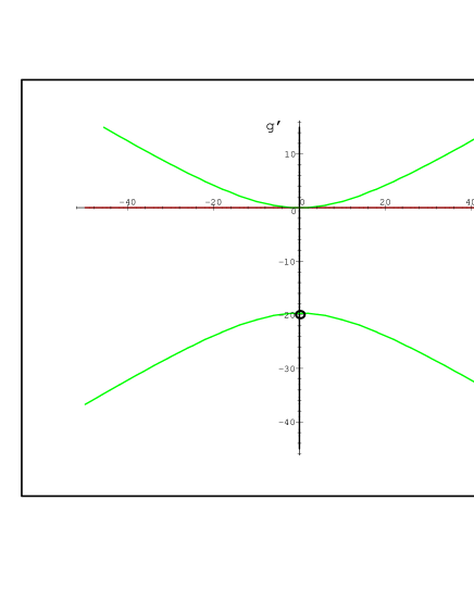
Figure 1: Fermionic parameter space.

We see that the manifold $g=0$ is present both in the classical and in the quantum case. This merely reflects the fact that massive Thirring model is integrable both classically and quantum mechanically. In contrast, the fermionic BL model (2.4), obtained by setting $g^{\prime}=0$ in the general action (2.1), has a charge of Lorentz spin 3 which is conserved classically but not quantum mechanically.

5 Conclusion

We have shown that the fermionic Bukhvostov–Lipatov model, given by the action (2.4), admits a nontrivial classical integral of motion of spin 3, both in the bulk and for specific types of boundary actions in the theory on the half line. This conservation law holds quantum mechanically only at the free fermion point $g=0$ and is spoiled by quantum corrections for generic values of the coupling $g$. The more general fermionic model (2.1) admits a quantum conservation law of spin 3 for the specific relation (4) between the couplings $g$ and $g^{\prime}$. The study of the spin 3 conservation laws, therefore, suggests that the integrable manifold $(g$ free, $g^{\prime}=0)$ proposed by Bukhvostov and Lipatov does not survive in the quantum field theory.

Appendix

The following is a list of boundary potentials for which the conservation of the spin 3 charge of the classical fermionic BL model is preserved in the theory on the half-line. This list does not claim to be exhaustive.

If one leaves out all additional boundary degrees of freedom, and considers the boundary actions which are functionals of the bulk fields only, the most general Ansatz for a boundary potential is:

$${\cal B}(\psi_{+}, \psi_{-},\overline{\psi}_{+},\overline{\psi}_{-};\chi_{+},\chi_{-},\overline{\chi}_{+},\overline{\chi}_{-})=$$

$$\ = a_{1}\psi_{-}\psi_{+}+a_{2}\overline{\psi}_{-}\overline{\psi}_{+}+b_{1}\chi_{-}\chi_{+}+b_{2}\overline{\chi}_{-}\overline{\chi}_{+}+$$

$$+ia_{3}\left[\psi_{-}\overline{\psi}_{-}-\overline{\psi}_{+}\psi_{+}\right]+ia_{4}\left[e^{i\alpha}\psi_{-}\overline{\psi}_{+}-e^{-i\alpha}\overline{\psi}_{-}\psi_{+}\right]+$$

$$+ib_{3}\left[\chi_{-}\overline{\chi}_{-}-\overline{\chi}_{+}\chi_{+}\right]+ib_{4}\left[e^{i\beta}\chi_{-}\overline{\chi}_{+}-e^{-i\beta}\overline{\chi}_{-}\chi_{+}\right]+$$

$$+ic_{1}\left[e^{i\gamma_{1}}\psi_{-}\chi_{-}-e^{-i\gamma_{1}}\chi_{+}\psi_{+}\right]+ic_{2}\left[e^{i\gamma_{2}}\psi_{-}\chi_{+}-e^{-i\gamma_{2}}\chi_{-}\psi_{+}\right]+$$

$$+id_{1}\left[e^{i\delta_{1}}\overline{\psi}_{-}\overline{\chi}_{-}-e^{-i\delta_{1}}\overline{\chi}_{+}\overline{\psi}_{+}\right]+id_{2}\left[e^{i\delta_{2}}\overline{\psi}_{-}\overline{\chi}_{+}-e^{-i\delta_{2}}\overline{\chi}_{-}\overline{\psi}_{+}\right]+$$

$$+if_{1}\left[e^{i\varphi_{1}}\psi_{-}\overline{\chi}_{-}-e^{-i\varphi_{1}}\overline{\chi}_{+}\psi_{+}\right]+if_{2}\left[e^{i\varphi_{2}}\psi_{-}\overline{\chi}_{+}-e^{-i\varphi_{2}}\overline{\chi}_{-}\psi_{+}\right]+$$

$$+if_{3}\left[e^{i\varphi_{3}}\overline{\psi}_{-}\chi_{-}-e^{-i\varphi_{3}}\chi_{+}\overline{\psi}_{+}\right]+if_{4}\left[e^{i\varphi_{4}}\overline{\psi}_{-}\chi_{+}-e^{-i\varphi_{4}}\chi_{-}\overline{\psi}_{+}\right]\ .$$

This Ansatz gives 8 linear equations of motion for the bulk fields at the boundary, depending on 26 real parameters, 16 amplitudes and 10 phases. In order to have non-trivial solution to this linear system we require that the $8\times 8$ matrix of coefficients be of rank 6 or smaller. Because of the size of the matrix it is difficult to study the problem in all its generality, but we list here some interesting particular cases:

1. No terms mixing the $\Psi$- and the $X$-fields appear in the boundary action, i.e. the coefficients $c_{1}$, $c_{2}$, $d_{1}$, $d_{2}$, $f_{1}$, $f_{2}$, $f_{3}$, and $f_{4}$ are equal to $0$. In this case the integrable boundary actions are linear combinations of the integral boundary actions for the MT model [9]:

$a_{1}$	$a_{2}$	$a_{3}$	$a_{4}$	$b_{1}$	$b_{2}$	$b_{3}$	$b_{4}$
$\frac{\tan\kappa_{0}}{2}$	$-\frac{\tan\kappa_{0}}{2}$	$\frac{1}{2\cos\kappa_{0}}$	$0$	$\frac{\tan\mu_{0}}{2}$	$-\frac{\tan\mu_{0}}{2}$	$\frac{1}{2\cos\mu_{0}}$	$0$
$\frac{\tan\kappa_{0}}{2}$	$-\frac{\tan\kappa_{0}}{2}$	$\frac{1}{2\cos\kappa_{0}}$	$0$	$\frac{\tan\nu_{0}}{2}$	$\frac{\tan\nu_{0}}{2}$	$0$	$\frac{1}{2\cos\nu_{0}}$
$\frac{\tan\lambda_{0}}{2}$	$\frac{\tan\lambda_{0}}{2}$	$0$	$\frac{1}{2\cos\lambda_{0}}$	$\frac{\tan\mu_{0}}{2}$	$-\frac{\tan\mu_{0}}{2}$	$\frac{1}{2\cos\mu_{0}}$	$0$
$\frac{\tan\lambda_{0}}{2}$	$\frac{\tan\lambda_{0}}{2}$	$0$	$\frac{1}{2\cos\lambda_{0}}$	$\frac{\tan\nu_{0}}{2}$	$\frac{\tan\nu_{0}}{2}$	$0$	$\frac{1}{2\cos\nu_{0}}$

where $\kappa_{0}$, $\lambda_{0}$, $\mu_{0}$, and $\nu_{0}$ are free real parameters $\neq\frac{k\pi}{2}$.

2. Only terms mixing the $\Psi$- and the $X$-fields are present. $a_{1}$, …, $a_{4}$ and $b_{1}$, …, $b_{4}$ are equal to $0$. If, in addition, we consider the even simpler sub-case when only terms mixing $\psi_{\pm}$ with $\overline{\chi}_{\pm}$ and $\overline{\psi}_{\pm}$ with $\chi_{\pm}$ are present, i.e. also $c_{1}$, $c_{2}$, $d_{1}$, $d_{2}$ vanish, the integrable boundary actions are given by:

$f_{1}$	$f_{2}$	$f_{3}$	$f_{4}$
$\frac{1}{2}\pm p_{0}$	$p_{0}$	$\frac{1}{2}\pm q_{0}$	$q_{0}$
$\pm\frac{1}{2}$	$0$	$r_{0}$	$s_{0}$
$0$	$\pm\frac{1}{2}$	$r_{0}$	$s_{0}$
$u_{0}$	$v_{0}$	$\pm\frac{1}{2}$	$0$
$u_{0}$	$v_{0}$	$0$	$\pm\frac{1}{2}$

where $p_{0}$, $q_{0}$, $r_{0}$, $s_{0}$, $u_{0}$, and $v_{0}$ are free real parameters. The integrable boundary actions of this type are specific for the boundary BL model.

References

• [1] A. P. Bukhvostov, L. N. Lipatov, Nucl. Phys. B180 (1981) 116.
• [2] V. A. Fateev, Nucl. Phys. B473 (1996) 509.
• [3] F. Lesage, H. Saleur, P. Simonetti, Phys. Rev. B56 (1997) 7598;
Phys. Rev. B57 (1998) 4694.
• [4] M. Ameduri, C. J. Efthimiou, J. Nonl. Math. Phys. 5 (1998) 132.
• [5] H. Saleur, “The Long Delayed Solution of the Bukhvostov–Lipatov Model”, hep-th/9811023.
• [6] S. Coleman, Phys. Rev. D11 (1975) 2088.
• [7] B. Berg, M. Karowski, H. J. Thun, Phys. Lett. B64 (1976) 286;
R. Flume, P. K. Mitter, N. Papanicolaou, Phys. Lett. B64 (1976) 289.
• [8] P. P. Kulish, E. R. Nisimov, JETP Lett. 24 (1976) 220;
R. Flume, S. Meyer, Lett. Nuovo Cimento 18 (1977) 238;
B. Berg, M. Karowski, H. J. Thun, Il Nuovo Cimento 38 (1977) 11.
• [9] T. Inami, H. Konno, Y.-Z. Zhang, Phys. Lett. B376 (1996) 90.
• [10] C. S. Gardner, J. M. Greene, M. D. Kruskal, R. M. Miura, Phys. Rev. Lett. 19 (1967) 1095.
• [11] P. D. Lax, Comm. Pure Appl. Math. 21 (1968) 467.
• [12] L. A. Takhtadzhyan, L. D. Faddeev, Theor. Math. Phys. 21 (1974) 1046.
• [13] L. Girardello, S. Sciuto, Phys. Lett. B77 (1978) 267.
• [14] S. Ferrara, L. Girardello, S. Sciuto, Phys. Lett. B76 (1978) 303.
• [15] J. N. G. N. Prata, Nucl. Phys. B496 (1997) 451.
• [16] M. Moriconi, A. De Martino, “Quantum Integrability of Certain Boundary Conditions”, hep-th/9809178.
• [17] S. Ghoshal, A. Zamolodchikov, Int. J. Mod. Phys. A9 (1994) 3841.
• [18] A. B. Zamolodchikov, Adv. Studies in Pure Math. 19 (1989) 641.