Abstract

After presenting a survey of theoretical results concerning the structure of two-dimensional QCD, we present a numerical study related to the mass eigenstates and the decay amplitudes of higher mesonic states. We discuss in detail the fate of important dynamical points such as stability of the spectrum and the problem of screening versus confinement in this context. We point out differences in the large distance behaviour of the potential, which can be responsible for the question of stability of the spectrum, as well as whether it is finite.

1 Introduction

Unlike the Schwinger model[1], Quantum Chromodynamics of massless fermions in two dimensions is not exactly solvable[2]. It nevertheless serves as a very useful laboratory for studying problems such as the bound-state spectrum and algebraic structure. These problems are important tools for general understanding of realistic quantum field theories and are expected to realize the important features of four dimensional Quantum Chromodynamics. In particular, exact properties may be derived, once one arrives at an equivalent bosonic formulation in the form of a gauged Wess-Zumino-Witten (WZW) action[3, 4].

The first attempt to obtain the particle spectrum dates back to 1974, and was based on the $1/N$ expansion[5, 6], where $N$ is the number of colours. In this limit one is led to a bound state spectrum corresponding asymptotically to a linearly rising Regge trajectory. The use of the principal-value prescription in dealing with the infrared divergencies is however highly ambiguous due to the non-commutative nature of principal-value integrals. Moreover, the result for the fermion propagator is tachyonic for a small fermion mass as compared with the coupling constant, hence, in particular, for zero fermion mass. This has made ’t Hooft’s solution a controversial issue[7].

In the large $N$ approximation the gluons remain massless, since fermion loops do not contribute to the Feynman amplitudes. This is unlike the $U(1)$ case, where the photon acquires a mass via an intrinsic Higgs mechanism. This has led to the speculations that $QCD_{2}$ may in fact exist in two phases associated with the weak and strong coupling regimes. In this picture, the large $N$ limit would correspond to the weak-coupling limit (’t Hooft’s phase), with massless gluons and a mesonic spectrum described by a Regge trajectory. In such a case, the Regge behaviour of the mesonic spectrum is compatible with confinement. In the strong coupling regime (Higgs phase), on the other hand, the gluons would be massive, and the original $SU(N)_{c}$-symmetry would be broken down to the maximal abelian subgroup (torus) of $SU(N)_{c}$.

The behaviour of the theory in the strong or weak coupling limits is rather subtle. The theory is asymptotically free. In the strong coupling limit, it is expected to be in the confining phase: in the infinite infrared cut-off limit quarks disappear from the spectrum, which consists of mesons lying approximately on a Regge trajectory.

The problem of screening and confinement can however be analysed along the lines of the $U(1)$ case. However, unlike the $U(1)$ case, the screening phase prevails in the non-abelian theory[8, 9].

1.1 QCD₂ in the local decoupled formulation and BRST constraints

The partition function of two-dimensional QCD in the fermionic formulation (before gauge fixing) is given by the expression

$${\cal Z}=\int{\cal D}A_{+}{\cal D}A_{-}\int{\cal D}\psi{\cal D}\bar{\psi}e^{iS[A,\psi,\bar{\psi}]}$$ (1)

with the action

$${\cal S}[\!A\!,\psi\!,\!\bar{\psi}\!]=\int\!d^{2}x\!\left[-\frac{1}{4}\!\mathop{\rm tr}F^{{}^{\mu\nu}}F_{{}_{\mu\nu}}+\psi^{\dagger}_{1}(i\partial_{+}+eA_{+})\psi_{1}+\psi^{\dagger}_{2}(i\partial_{-}+eA_{-})\psi_{2}\right].$$ (2)

We can obtain a bosonic formulation of the theory, in such a way that structural relations, hidden in the fermionic formulation are made clearer in the bosonic counterpart. We first make some useful change of variables, obtaining a formulation in terms of matrix-valued fields which decouple at the partition function level, but which are not totally decoupled, due to the gauge symmetries of the theory.

We can also arrive at a factorized form of the partition function (1) by parametrizing $A_{\pm}$ as

$$eA_{+}=U^{-1}i\partial_{+}U\quad,\quad A_{-}=Vi\partial_{-}V^{-1}$$ (3)

as well as performing a chiral rotation,

$$\psi_{1}\to\psi_{1}^{(0)}\equiv U\psi_{1},\quad\psi_{2}\to\psi_{2}^{(0)}=V^{-1}\psi_{2}\quad.$$ (4)

We arrive at

$${\cal Z}={\cal Z}_{F}^{(0)}\int{\cal D}U{\cal D}W{\cal J}_{G}[W]{\cal J}_{F}[W]e^{i{\cal S}_{YM}[W]}\quad,$$ (5)

where ${\cal Z}^{(0)}_{F}$ is the partition function of free fermions, and ${\cal S}_{YM}$ is the Yang-Mills action given by

$${\cal S}_{YM}[W]=\int d^{2}x[E^{2}+E\partial_{+}(Wi\partial_{-}W^{-1})]$$ (6)

with $W=UV$.

The field strength tensor $F_{01}$ is given in terms of $W$ and $U$ or $V$ in either of the two alternative forms

$$F_{01}=-\frac{1}{2}U^{-1}[\partial_{+}(Wi\partial_{-}W^{-1})]U=\frac{1}{2}V[\partial_{-}(W^{-1}i\partial_{+}W)]V^{-1}\quad.$$ (7)

The Jacobian ${\cal J}_{F}$ is given, following Fujikawa, by

$${\cal J}_{F}[UV]=e^{-i\Gamma[UV]}$$ (8)

while the determinant of the adjoint Dirac operator is

$${\cal J}_{G}[UV]=e^{-ic_{V}\Gamma[UV]}(\det i\partial_{+})_{adj}(\det i\partial_{-})_{adj}\quad,$$ (9)

where $c_{V}$ is the second Casimir of the group in question with the normalization $f_{acd}f_{bcd}=c_{V}\delta_{ab}$ of the structure constants, and $\Gamma[UV]$ is the Wess-Zumino-Witten action. Representing $(\det i\partial_{\pm})_{adj}$ in terms of ghosts and choosing the gauge $U=1$, we obtain

$${\cal Z}={\cal Z}^{(0)}_{F}{\cal Z}^{(0)}_{gh}{\cal Z}_{W}\quad,$$ (10)

where ${\cal Z}^{(0)}_{gh}={\cal Z}^{(0)}_{gh+}{\cal Z}^{(0)}_{gh-}$ and

$${\cal Z}_{W} = \int{\cal D}We^{-i(1+c_{V})\Gamma[W]}e^{i{\cal S}_{YM}[W]}=\int{\cal D}We^{iS_{eff}[W]}\quad,$$ (11)

where we introduced the $W$–effective action

$$S_{eff}[W] = S_{YM}-(c_{V}+1)\Gamma[W]\quad.$$ (13)

The effective action has two terms, one corresponding to a WZW action with a negative coefficient, and the Yang-Mills action written in the form (6).

We refer to (10) as the “local decoupled” partition function. As seen from (11), the ghosts $b_{\pm}^{(0)}$ are canonically conjugate to $c_{\pm}^{(0)}$ and have Grassmann parity $+1$. We assign to them the ghost number $gh\#=-1$ and $gh\#=+1$, respectively.

The dimensionality of the direct-product space ${\cal H}_{F}^{(0)}\otimes{\cal H}_{gh}^{(0)}\otimes{\cal H}_{W}$ associated with the partition function (10) is larger than that of the physical Hilbert space of the original fermionic formulation. Hence there must exist constrains imposing restrictions on the representations which are allowed in ${\cal H}_{phys}$. In order to discover these constraints we observe that the partition function is separately invariant under the following nilpotent transformations [10, 11]
$\displaystyle W\delta W^{-1}=-c_{-}^{(0)}\;,$ $\displaystyle\delta\psi^{(0)}_{1}=c_{-}^{(0)}\psi_{1}^{(0)}\;,\;\delta\psi^{(0)}_{2}=0\;,$ $\displaystyle\delta c_{-}^{(0)}=\frac{1}{2}\{c_{-}^{(0)},c_{-}^{(0)}\}\;,\;\delta c_{+}^{(0)}=0\;,$ $\displaystyle\delta b^{(0)}_{-}=\Omega_{-}\;,\;\delta b_{+}^{(0)}=0\quad,$ $\displaystyle W^{-1}\delta W=-c_{+}^{(0)}\;,$ $\displaystyle\delta\psi_{1}^{(0)}=0\;,\;\delta\psi_{2}^{(0)}=c_{+}^{(0)}\psi_{2}^{(0)}\;,$ $\displaystyle\delta c^{(0)}_{-}=0\;,\;\delta c_{+}^{(0)}=\frac{1}{2}\left\{c_{+}^{(0)},c_{+}^{(0)}\right\}\;,$ $\displaystyle\delta b_{-}^{(0)}=0\;,\;\delta b_{+}^{(0)}=\Omega_{+}\;,$
where $\delta$ denotes the variation graded with respect to Grassmann parity, and $\Omega_{\mp}$ are given by
$\displaystyle\Omega_{-}$ $\displaystyle=$ $\displaystyle-\frac{1}{4e^{2}}{\cal D}_{-}(W)(\partial_{+}(Wi\partial_{-}W^{-1}))-\left({1+c_{V}}\right)J_{-}(W)+j_{-}$ $\displaystyle\Omega_{+}$ $\displaystyle=$ $\displaystyle-\frac{1}{4e^{2}}{{\cal D}}_{+}(W)(\partial_{-}(W^{-1}i\partial_{+}W))-\left(1+c_{V}\right)J_{+}(W)+j_{+}$
with

$$J_{-}(W)={1\over 4\pi}Wi\partial_{-}W^{-1}\,,\quad J_{+}(W)={1\over 4\pi}W^{-1}i\partial_{+}W\;,$$ (16)

$$j_{-}=\psi_{1}^{(0)}\psi_{1}^{(0)\dagger}+\{b_{-}^{(0)},c_{-}^{(0)}\}\,,\quad j_{+}=\psi_{2}^{(0)}\psi_{2}^{(0)\dagger}+\{b_{+}^{(0)},c_{+}^{(0)}\}\;.$$ (17)

These transformations are easily derived by departing from the Yang-Mills action[10, 11].

The corresponding BRST currents, as obtained via the usual Noether construction, are found to be

$$J_{\mp}=\mathop{\rm tr}c^{(0)}_{-}\left[\Omega_{\mp}-\frac{1}{2}\{b_{\mp}^{(0)},c_{\mp}^{(0)}\}\right]\quad,$$ (18)

with $\partial_{+}J_{-}=0$, and $\partial_{-}J_{+}=0$.

Remarkably enough, the nilpotent symmetries lead to currents $J_{-}$ and $J_{+}$ which only depend on the variable $x^{-}$ and $x^{+}$, respectively.

The on-shell nilpotency of the corresponding conserved charges

$$Q_{\pm}=\int dx^{1}J_{\pm}(x^{\pm})$$ (19)

follows from the first-class character of the operators $\Omega^{a}_{\pm}=\mathop{\rm tr}\left(t^{a}\Omega_{\pm}\right)$.

1.2 $QCD_{2}$ in the non-local decoupled formulation and BRST constraints

The partition function represented by the standard expression (11) contains fields which are mixtures of massive and massless modes, of positive and negative norms respectively, coupled by the constraints. In the following we dissociate these degrees of freedom by a suitable transformation. We shall thereby be lead to an alternative nonlocal representation of the partition function, useful for learning certain structural properties.

Following Ref. [12], we make in (6) the change of variables $E\to\beta$ defined by

$$\partial_{+}E=\left(\frac{1+c_{V}}{2\pi}\right)\beta^{-1}i\partial_{+}\beta\quad.$$ (20)

The Jacobian associated with this change of variables is

$${{\cal D}}E=\det i{\cal D}_{+}(\beta){{\cal D}}\beta$$ (21)

where we have suppressed the constant $\det\partial_{+}$ which will not play any role in the discussion to follow. Making use of the determinant of the fermionic operator in the fundamental or in the adjoint representation and representing $\left(\det i\partial_{+}\right)$ as a functional integral over ghost fields $\hat{b}_{-}$ and $\hat{c}_{-}$, we have, after decoupling the ghosts,

$${\cal Z} = {\cal Z}_{F}^{(0)}{\cal Z}_{gh}^{(0)}\hat{\cal Z}_{gh-}^{(0)}\int{\cal D}W\int{\cal D}\beta\exp\{-i(1+c_{V})[\Gamma[W]+\Gamma[\beta]$$

$$-\frac{1}{4\pi}\int tr(\beta^{-1}\partial_{+}\beta W\partial_{-}W^{-1})]\}$$

$$\times\exp({i\Gamma[\beta]})\exp\left\{{i\left(\frac{1+c_{V}}{2\pi}\right)^{2}e^{2}\int\frac{1}{2}tr\left[\partial^{-1}_{+}(\beta^{-1}\partial_{+}\beta\right]^{2}}\right\}\quad,$$

where

$$\hat{\cal Z}_{gh-}^{(0)}=\int{\cal D}\hat{b}^{(0)}_{-}{\cal D}\hat{c}_{-}^{(0)}e^{i\int d^{2}x\mathop{\rm tr}\hat{b}_{-}^{(0)}i\partial_{+}\hat{c}^{(0)}_{-}}\quad.$$ (23)

Using the Polyakov-Wiegmann identity, [2] and making the change of variable $W\to\beta W=\tilde{W}$, we are left with

$${\cal Z}={\cal Z}^{(0)}_{F}{\cal Z}^{(0)}_{gh}\hat{\cal Z}_{gh-}^{(0)}{\cal Z}_{\tilde{W}}{\cal Z}_{\beta}\quad,$$ (24)

where

$${\cal Z}_{\beta}=\int{{\cal D}}\beta\exp\left\{{i\Gamma[\beta]+i\left(\frac{1+c_{V}}{2\pi}\right)^{2}e^{2}\int\frac{1}{2}tr\left[\partial_{+}^{-1}(\beta^{-1}\partial_{+}\beta)\right]^{2}}\right\}$$ (25)

and

$${\cal Z}_{\tilde{W}}=\int{\cal D}\tilde{W}\exp[{-i(1+c_{V})\Gamma[\tilde{W}]}]$$ (26)

is the partition function of a WZW field of level $-(1+c_{V})$.

1.3 Massive two-dimensional QCD

The BRST symmetries of the physical states in massless QCD₂ are also the symmetries which should be imposed on the physical states in the massive case. For massive fermions the functional determinant of the Dirac operator, an essential ingredient for arriving at the bosonised form of the QCD₂ partition function, can no longer be computed in closed form, and one must resort to the so-called adiabatic principle of form invariance[2]. Equivalently, one can start with a perturbative expansion in powers of the mass, as given by

$$\sum{1\over n!}M^{n}\left[\int{\rm d}^{2}x\overline{\psi}\psi\right]^{n}\quad.$$ (27)

Afterwards, we use the (massless) bosonization formulae and re-exponentiate the result. In this approach, the mass term is given in terms of a bosonic field $g_{\psi}$ of the massless theory by[13]

$$S_{m}=-M\int\overline{\psi}\psi=M\mu\int\mathop{\rm tr}(g_{\psi}+g_{\psi}^{-1})\quad,$$

where $\mu$ is an arbitrary massive parameter whose value depends on the renormalization prescription for the mass operator.[2]

Defining $m^{2}=M\mu$, we re-exponentiate the mass term. Going through the changes of variables leading to (24), one arrives at the following alternative forms for the mass term when expressed in terms of the fields of the non-local formulation

$$S_{m}=m^{2}\int\mathop{\rm tr}(g\tilde{\Sigma}^{-1}\beta+\beta^{-1}\tilde{\Sigma}g^{-1})\quad.$$ (28)

The corresponding effective action of massive QCD₂ in the non-local formulation reads

$$S=S_{YM}[\beta,B]+S_{m}[g,\beta,\tilde{\Sigma}]+\Gamma[g]+\Gamma[\beta]-(c_{V}+1)\Gamma[\tilde{\Sigma}]+S_{gh}+\hat{S}_{gh-}\quad.$$ (29)

We thus see that the associated partition function no longer factorizes. Nevertheless, there still exist BRST currents which are either right- or left-moving, just as in the massless case.

The action (29) exhibits various symmetries of the BRST type; however, not all of them lead to nilpotent charges. The variations are graded with respect to Grassmann number. The equations of motion obtained from action (29) read

$${1\over 4\pi}\partial_{+}(g\partial_{-}g^{-1})= m^{2}(g\tilde{\Sigma}^{-1}\beta-\beta^{-1}\tilde{\Sigma}g^{-1})\;,$$ (30)

$$-{c_{V}+1\over 4\pi}\partial_{+}(\tilde{\Sigma}\partial_{-}\tilde{\Sigma}^{-1})=\, m^{2}(\tilde{\Sigma}g^{-1}\beta^{-1}-\beta g\tilde{\Sigma}^{-1})\;,$$ (31)

$${1\over 4\pi}\partial_{+}(\beta\partial_{-}\beta^{-1})+i\lambda\partial_{+}(\beta B\beta^{-1})=\, m^{2}(\beta g\tilde{\Sigma}^{-1}-\tilde{\Sigma}g^{-1}\beta^{-1})\;,$$ (32)

$$-{1\over 4\pi}\partial_{-}(\beta^{-1}\partial_{+}\beta)+ i\lambda[\beta^{-1}\partial_{+}\beta,B]+$$

$$i\lambda\partial_{+}B=\, m^{2}(g\tilde{\Sigma}^{-1}\beta-\beta^{-1}\tilde{\Sigma}g^{-1})\quad,$$ (33)

$$\partial_{+}^{2}B=\, \lambda(\beta^{-1}i\partial_{+}\beta)\;,$$ (34)

$$\partial_{\pm}b_{\mp}=\, 0\quad,\quad\partial_{\pm}c_{\mp}=0\quad,$$ (35)

with an analogous set of equations involving a so called prime sector[10], and where $\lambda=\frac{c_{V}+1}{2\pi}e$. Notice that the mass term can be transformed from one equation to another, by a suitable conjugation. Making use of Eqs. (30-35), the Noether currents are constructed in the standard fashion: we make a general BRST variation of the action, without using the equations of motion, and equate the result to the on-shell variation, taking into account terms arising from partial integrations. The only subtlety in this procedure concerns the WZW term, which only contributes off-shell to the variation. The four conserved Noether currents are found to be

$$J_{\pm}=\, \mathop{\rm tr}\left(c_{\pm}\Omega_{+}-{1\over 2}b_{\pm}\{c_{\pm},c_{\pm}\}\right)\quad,$$ (36)

$$\hat{J}_{\pm}=\, \mathop{\rm tr}\left(\hat{c}_{\pm}\hat{\Omega}_{\pm}-{1\over 2}\hat{b}_{\pm}\{\hat{c}_{\pm},\hat{c}_{\pm}\}\right)\quad,$$ (37)

where the constraints above generally denoted as $\Omega$ are given by

$$\Omega_{+} = \left({1\over 4\pi}g^{-1}i\partial_{+}g-{c_{V}+1\over 4\pi}\tilde{\Sigma}^{-1}i\partial_{+}\tilde{\Sigma}+\{b_{+},c_{+}\}\right)\quad,$$ (38)

$$\Omega_{-} = \left({1\over 4\pi}gi\partial_{-}g^{-1}-{c_{V}+1\over 4\pi}\tilde{\Sigma}^{\prime}i\partial_{-}\tilde{\Sigma}^{\prime-1}+\{b_{-},c_{-}\}\right)\quad,$$ (39)

$$\hat{\Omega}_{-} = \left({1\over 4\pi}\beta i\partial_{-}\beta^{-1}-{c_{V}+1\over 4\pi}\tilde{\Sigma}i\partial_{-}\tilde{\Sigma}^{-1}-\lambda\beta B\beta^{-1}+\{b_{-},c_{-}\}\right)\quad,$$ (40)

$$\hat{\Omega}_{+} = \!\left(\!{1\over 4\pi}\!\beta^{\prime-1}i\partial_{+}\beta^{\prime}\!-\!{c_{V}+1\over 4\pi}\tilde{\Sigma}^{\prime-1}i\partial_{+}\tilde{\Sigma}^{\prime}\!-\!\lambda\beta^{\prime-1}B^{\prime}\beta^{\prime}\!+\!\{\hat{b}_{+},\hat{c}_{+}\}\right)\,.$$ (41)

(see [10, 11] for definitions concerning the primed sector, connected to the unprimed one by a nonlocal transformation).

From the current conservation laws

$$\partial_{\mp}J_{\pm}=0\quad,\quad\partial_{\pm}\hat{J}_{\mp}=0\quad,$$ (42)

one infers that $\Omega_{-}$ and $\hat{\Omega}_{-}$ are right-moving, while $\Omega_{+}$ and $\hat{\Omega}_{+}$ are left-moving. Indeed, making use of the equations of motion (30-35) one readily checks that the operators $\Omega_{\pm}$, $\hat{\Omega}_{\pm}$ satisfy

$$\partial_{\mp}\Omega_{\pm}=0\quad,\quad\partial_{\pm}\hat{\Omega}\mp=0\quad,$$ (43)

consistent with the conservation laws (42). In Ref. [10] it has been argued that gauge invariant bilinears are the physical states of the theory. There is of course the problem of whether we have to consider or not that the physical states are annihilated by the non local constraints, but that problem goes beyond the scope of the present paper.

1.4 Screening in two-dimensional QCD

Let us reconsider the problem of screening and confinement. We shall concentrate on the case of single flavour QCD, and merely comment on the general case at the end of the section.

We proceed by first considering the case of massless fermions and compute the inter-quark potential. We introduce a pair of classical colour charges of strength $q=q^{a}t^{a}$ separated by a distance $L$. Such a pair is introduced in the action (29) by means of the substitution

$$i(\beta^{-1}\partial_{+}\beta)^{a}\longrightarrow i(\beta^{-1}\partial_{+}\beta)^{a}-{2\pi\over e}q^{a}\bigg{(}\delta(x-{L\over 2})-\delta(x+{L\over 2})\bigg{)}\quad,$$ (44)

where $a$ is a definite colour index. This adds the following term to the action

$$V(L)=\Delta S=S_{q}-S=-(c_{V}+1)q^{a}\bigg{(}B^{a}(L/2)-B^{a}(-L/2)\bigg{)}\quad.$$ (45)

The equation of motion for $B^{a}$ is now replaced by

$$\partial_{+}^{2}B^{a}=i\lambda(\beta^{-1}\partial_{+}\beta)^{a}-(c_{V}+1)q^{a}\bigg{(}\delta(x-{L\over 2})-\delta(x+{L\over 2})\bigg{)},$$ (46)

which implies, upon substitution into the equation of motion for the $\beta$-field,

$$\partial_{+}\left({i\over 4\pi\lambda}\partial_{-}\partial_{+}B+[\partial_{+}B,B]+i\lambda B\right)=$$

$$\qquad\left({-iq\over 2e}\partial_{-}+(c_{V}+1)[q,B]\right)[\delta(x-{L\over 2})-\delta(x+{L\over 2})]\quad.$$ (47)

We look for solutions of (47) with a fixed global orientation in colour space. We thus make $B^{a}=q^{a}f(x)$. This renders the problem abelian. We thus infer that the potential (45) has the form

$$V(L)={(c_{v}+1)\sqrt{\pi}\over 2}{q^{2}\over e}(1-e^{-2\sqrt{\pi}\lambda L})$$ (48)

which implies that the system is in a screening phase.

We now turn to the case of massive fermions. Taking the external charge to lie in the direction $t^{2}$ of $SU(N)$ space, our Ansatz for $B^{a}$ leads one to look for solutions with $g$, $\beta$ and $\Sigma$ parametrized as

$$g=e^{i2\sqrt{\pi}\varphi\sigma_{2}},\qquad\beta=e^{i2\sqrt{\pi}E\sigma_{2}},\qquad\Sigma=e^{-i2\sqrt{\pi}\eta\sigma_{2}}\quad.$$ (49)

The equations of motion (30-34) are replaced by a set of coupled sine-Gordon type equations. As is well known[2], the solution of the classical equations of motion in the bosonic version contains quantum mechanical information from the fermionic theory. We find, after solving them, the result[9]

$$V(L)={(c_{V}+1)^{2}q^{2}\over 2}\times$$

$$\left[\left({4\pi\lambda^{2}-m_{-}^{2}\over m_{+}^{2}-m_{-}^{2}}\right)\!\!\!\left({1-e^{-m_{+}L}\over m_{+}}\right)+\left({m_{+}^{2}-4\pi\lambda^{2}\over m_{+}^{2}-m_{-}^{2}}\right)\left({1-e^{-m_{-}L}\over m_{-}}\right)\right]\;,$$ (50)

where

$$\epsilon = {c_{V}\over(c_{V}+1)}\quad,\quad q_{+}={2\sqrt{\pi}(c_{V}+1)q\over(1+\epsilon a^{2})}\;,$$

$$a = -{8\pi m^{2}\over m_{+}^{2}-16\epsilon m^{2}}\quad,\quad q_{-}={2\sqrt{\pi}\epsilon a(c_{V}+1)q\over(1+\epsilon a^{2})}$$ (51)

$$m_{\pm}^{2} = 2\pi[\left(\lambda^{2}+(1+\epsilon)2m^{2}\right)\pm\sqrt{\left(\lambda^{2}+(1+\epsilon)2m^{2}\right)^{2}-8\epsilon\lambda^{2}m^{2}}],$$

$$Q_{\pm} = q_{\pm}\left[\Theta(x-{L\over 2})-\Theta(x+{L\over 2})\right]\;.$$ (52)

Thus we find two mass scales given by $m_{+}$ and $m_{-}$. Both these scales correspond to screening-type contributions if $c_{V}\not=0$.

Next, we compare the above results for the potential with those obtained for the Schwinger model. In the abelian case, the combination of the matter boson $\varphi$ and the negative metric scalar $\eta$ gives rise to the $\theta$-angle. That is, the combination $\Phi\equiv\varphi+\eta=\theta$ appears in the mass term. When fermions are massless, the electric field and the matter boson decouple. However, due to a Higgs mechanism, the electric field acquires a mass and, therefore, a long-range force does not exist. This leads to a pure screening potential. On the other hand, for massive fermions, the electric field couples to the matter boson $\Phi$. Yet, $\Phi=\psi_{c_{V}=0}$, and hence, it remains massless. The coupling to $\Phi$ via the mass term is the origin of the long-range force (linearly rising potential) in the massive U(1) case, where the potential is confining. On the other hand, the expression (50) for the potential indicates the absence of a long-range force in the non-abelian case.

The abelian potential can also be obtained from (50) by taking the limit $c_{V}\to 0$. In this limit, the mass scale $m_{-}$ tends to zero and we recover the linearly rising potential, signaling confinement.

1.5 Equations of motion and higher conservation equations

We are now going to deal with the action $S_{eff}$ given in (11), obtaining further important information.

Due to the presence of higher derivatives in that action, it is convenient to introduce an auxiliary field and rewrite it in the equivalent form (6).

The equation of motion of the $W$-field is easily computed. The WZW contribution has been obtained in [14], and the Yang-Mills action leads to an extra term. We obtain

$$[{c_{V}+1\over 4\pi}\partial_{+}+\frac{\partial_{+}\partial_{-}}{(4\pi\mu)^{2}}]\left(W\partial_{-}W^{-1}\right)-\frac{\partial_{+}}{(4\pi\mu)^{2}}[W\partial_{-}W^{-1},\partial_{+}\left(W\partial_{-}W^{-1}\right)]\equiv$$

$$[{c_{V}+1\over 4\pi}\partial_{+}+{1\over(4\pi\mu)^{2}}\partial_{+}{\cal D}_{-}]\left(W\partial_{-}W^{-1}\right)=0.$$ (53)

We can list the relevant field operators appearing in the definition of the conservation law (53), that is

$$I^{W}_{-}={1\over 4\pi}(c_{V}+1)J^{W}_{-}+{1\over(4\pi\mu)^{2}}\partial_{+}\partial_{-}J^{W}_{-}-{1\over(4\pi\mu)^{2}}[J^{W}_{-},\partial_{+}J^{W}_{-}]\quad,$$ (54)

with $\partial_{+}I^{W}_{-}=0$, and $J^{W}_{-}=W\partial_{-}W^{-1}$. It is straightforward to compute the Poisson algebra, using the canonical formalism, which in the bosonic formulation includes quantum corrections. We have

$$\left\{I^{W}_{ij}(t,x),I^{W}_{kl}(t,y)\right\} = I^{W}_{[kj}\delta_{il]}\delta(x^{1}\!-\!y^{1})-\alpha\delta^{il}\delta^{kj}\delta^{\prime}(x^{1}-y^{1})\quad,$$

$$\left\{I^{W}_{ij}(t,x),J^{W}_{-kl}(t,y)\right\} = J^{W}_{-[kj}\delta_{il]}\delta(x^{1}-y^{1})+2\delta_{il}\delta_{kj}\delta^{\prime}(x^{1}-y^{1})\quad,$$

$$\left\{J^{W}_{ij}(t,x),J^{W}_{-kl}(t,y^{1})\right\} = 0\quad,$$ (55)

where $\alpha={1\over 2\pi}(c_{V}+1)$, and the indices in the right hand side have been appropriately antisimetrized, as denoted by the bracketts in the indices of the current $I$ and of the Kronecker delta $\delta_{ij}$. We thus obtain a current algebra for $I_{-}^{W}$, acting on $J^{W}_{-}$ with a central extension.

1.6 Dual case-non local formulation

At the Lagrangian level, we find the Euler-Lagrange equations for $\beta$ from the perturbed WZW action (25), that is,

$$\delta\Gamma[\beta] = \left[{1\over 4\pi}\partial_{-}(\beta^{-1}\partial_{+}\beta)\right]\beta^{-1}\delta\beta\quad,$$ (56)

$$\delta\Delta(\beta) = 2\Big{(}\partial_{+}^{-1}(\beta^{-1}\partial_{+}\beta)-\big{[}\partial_{+}^{-2}(\beta^{-1}\partial_{+}\beta),(\beta^{-1}\partial_{+}\beta)\big{]}\Big{)}\beta^{-1}\delta\beta\quad.$$ (57)

We define the current components

$$J_{+}^{\beta} = \beta^{-1}\partial_{+}\beta\quad,$$ (58)

$$J_{-}^{\beta} = -4\pi\mu^{2}\partial_{+}^{-2}J_{+}^{\beta}=-4\pi\mu^{2}\partial_{+}^{-2}(\beta^{-1}\partial_{+}\beta)\quad,$$ (59)

which summarize the $\beta$ equation of motion as a zero-curvature condition given by

$$[{\cal L},{\cal L}]=[\partial_{+}+J_{+}^{\beta},\partial_{-}+J_{-}^{\beta}]=\partial_{-}J_{+}^{\beta}-\partial_{+}J_{-}^{\beta}+[J_{-}^{\beta},J_{+}^{\beta}]=0\quad.$$ (60)

This is not a Lax pair, as e.g. in the usual non-linear $\sigma$-models, where $J^{\beta}_{\mu}$ is a conserved current and a conserved non-local charge is obtained. However, to a certain extent, the situation is simpler in the present case, due to the rather unusual form of the currents. This permits us to write the commutator as a total derivative, in such a way that in terms of the current $J_{-}^{\beta}$ we have

$$\partial_{+}\left(4\pi\mu^{2}J_{-}^{\beta}+\partial_{+}\partial_{-}J_{-}^{\beta}+[J_{-}^{\beta},\partial_{+}J_{-}^{\beta}]\right)=0\quad.$$ (61)

Therefore the quantity

$$I_{-}^{\beta}(x^{-})=4\pi\mu^{2}J_{-}^{\beta}(x^{+},x^{-})+\partial_{+}\partial_{-}J_{-}^{\beta}(x^{+},x^{-})+[J_{-}^{\beta}(x^{+},x^{-}),\partial_{+}J_{-}^{\beta}(x^{+},x^{-})]\quad$$ (62)

does not depend on $x^{+}$, and it is a simple matter to derive an infinite number of conservation laws from the above.

Canonical quantization proceeds straightforwardly, and as a consequence we can compute the algebra of conserved currents, which is analogous to (55).

We are thus led to speculate whether two-dimensional QCD contains an integrable system[2]. The theory corresponds to an off-critical perturbation of the WZW action. If we write $\beta={\rm e}^{i\phi}\sim 1+i\phi$, we verify that the perturbing term corresponds to a mass term for $\phi$. The next natural step is to obtain the algebra obeyed by (62), and its representation. However, there is a difficulty presented by the non-locality of the perturbation.

1.7 Algebraic aspects of QCD₂ and integrability

We saw that two-dimensional QCD, although not exactly soluble, in terms of free fields, is a theory from which some valuable results may be obtained. The $1/N$ expansion reveals a simple spectrum valid for weak coupling, while the strong coupling offers the possibility of understanding the baryon as a generalized sine-Gordon soliton.

All such results point to a relatively simple structure, which could be mirrored by an underlying spectrum generating algebra. In fact such an algebra does exist. In the above-mentioned case of the large-$N$ expansion of pure QCD₂, one finds a $W_{\infty}$ spectrum generating algebra related to area-preserving diffeomorphisms of the Nambu-Goto action. For gauge-invariant bilinears in the Fermi fields this algebra can be constructed [15]. It also appears in the description of the quantum Hall effect. Moreover, pure QCD₂ is equivalent to the $c=1$ matrix model, which also has a representation in terms of non-relativistic fermions. The problem is also related to the Calogero-Sutherland models. The mass eigenstates build a representation of the $W_{\infty}$ algebra as found in [15].

In spite of the hints toward a possible integrable structure in two-dimensional QCD the problem still remains largely open[16]. A possible explanation was also given in [17]. The problem points to a better understanding of the mesonic spectrum of the theory. ’t Hooft’s results implying an infinite number of mesons obeying Regge behaviour is compatible with confinement. However, results obtained by several authors [8, 9, 18] point to a screening phase. In that case the quark anti-quark potential looks too shallow to support an infinite number of bound states.

Here we investigate the decay amplitudes of two-dimensional QCD using a refined numerical analysis, which will permit to account for the details of the dynamics.

2 Numerical backup

We have investigated the behaviour of the decay amplitudes of ’t Hooft mesons in the theory, in the large $N$ limit.

One of the strong reasons to study decay amplitudes is to learn about the stability of the ’t Hooft mesons, namely answer whether they might represent soliton solutions of two-dimensional QCD. Moreover, these mesons are a probe into the long range force: indeed, if two-dimensional QCD is confining there is a linearly rising potential which acomodates an infinite number of bound states. On the other hand, screening would imply a shallow potential, flatening at infinity, implying a finite number of mesons.

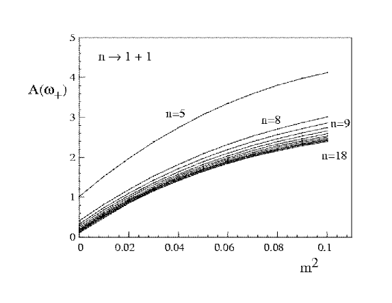
Fig. 1: Amplitudes for the decay processes $n\rightarrow 1+1$ ($n=5,8,9,\ldots,18$) versus the squared fermion mass $m^{2}$, varying from 0 to 0.1.

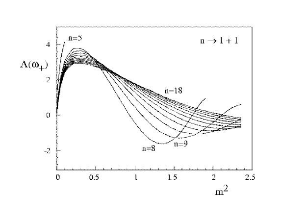
Fig. 2: Amplitudes for the decay processes $n\rightarrow 1+1$ ($n=5,8,9,\ldots,18$) versus the squared fermion mass $m^{2}$, varying from 0 to 2.35.

Decay amplitudes in the framework of perturbation theory in the inverse number of colours has been studied by a few authors [19]. The essential ingredient is first the solution of ’t Hooft equation in order to find the bound state wave functions and meson mass-square eigenvalues $\mu^{2}$:

$$\mu^{2}\phi(x)=\frac{\gamma-1}{x(1-x)}\phi(x)-P\int_{0}^{1}dy\frac{\phi(y)}{(x-y)^{2}}~{},$$ (63)

where $P$ denotes de Cauchy principal value prescription. Here $\gamma$ refers to a square mass scale corresponding to the quark-antiquark pair with equal masses $m^{2}$, where the massless limit is obtained for $\gamma=0$ [6].

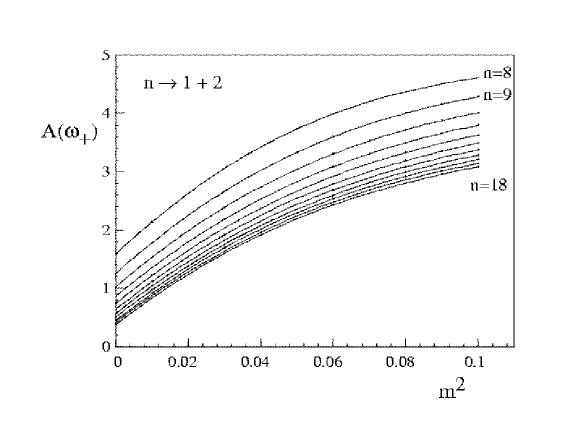
Fig. 3: As in figure 1, for the decay processes $n\rightarrow 1+2$ ($n=8,9,\ldots,18$).

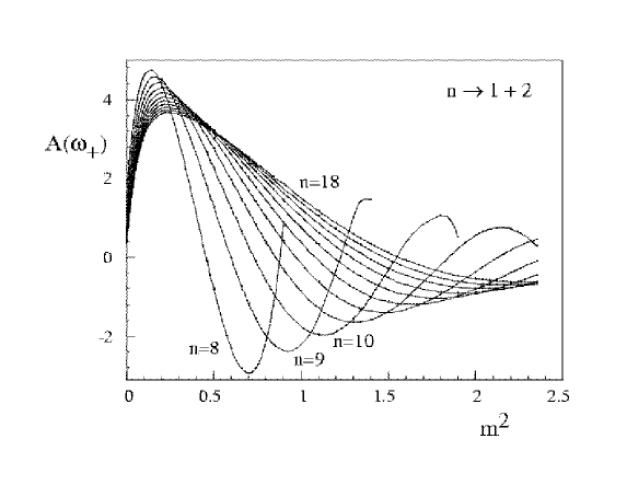
Fig. 4: As in figure 2, for the decay processes $n\rightarrow 1+2$ ($n=8,9,\ldots,18$).

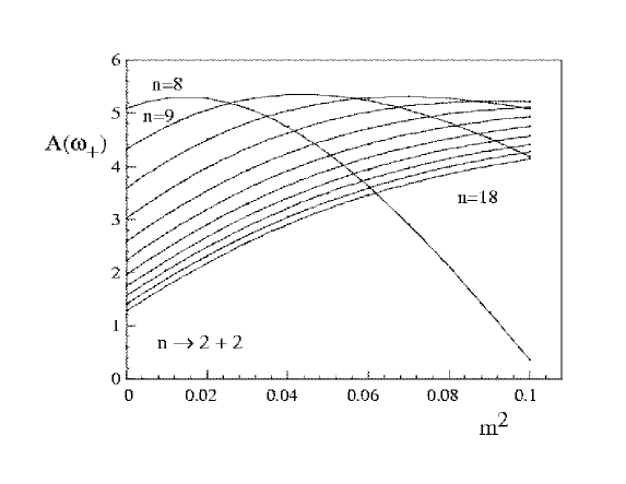
Fig. 5: As in fig. 1, for the decay processes $n\rightarrow 2+2$ ($n=8,9,\ldots,18$).

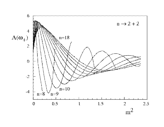
Fig. 6: As in figure 2, for the decay processes $n\rightarrow 2+2$ ($n=8,9,\ldots,18$).

This integro differential equation cannot be solved by analytic methods. However, using a sensible numerical method presented in [20] one can arrive at quite reasonable results for the eigenvalues and wave functions. This method makes use of a spline procedure to work out the exact wave functions on an adaptive grid. The numerical representation of the eigenfunctions are used to evaluate the decay amplitudes from an initial meson state $n$ into two final states $n_{1}$ and $n_{2}$. In the leading and next to leading order in the $1/N$ expansion they are given by [21, 22]

$$\langle n|n_{1},n_{2}\rangle = (1-C)\frac{1}{1-w}\int_{0}^{w}dx\phi_{n}(x)\phi_{n_{1}}(\frac{x}{w})\Phi_{n_{2}}(\frac{x-w}{1-w})$$ (64)

$$-(1-C)\frac{1}{w}\int_{w}^{1}dx\phi_{n}(x)\phi_{n_{2}}(\frac{x-w}{1-w})\Phi_{n_{1}}(\frac{x}{w})$$

$$+\frac{1}{N}(1-C)\frac{f_{n_{2}}}{1-w}\int_{0}^{w}dx\phi_{n}(x)\phi_{n_{1}}(\frac{x}{w}),$$

where $C$ denotes de interchange of final states,

$$\Phi_{n}(x)=\int_{0}^{1}dy\frac{\phi_{n}(y)}{(x-y)^{2}}$$ (65)

and $w$ is a kinematic parameter, whose on-shell values $w_{+}$ and $w_{-}$ correspond to the right moving and left moving of the final state $n_{1}$.

As observed in [17] the higher-order corrections for the amplitude are always multiplied by the factor

$$f_{n_{2}}=\int_{0}^{1}dx\phi_{n_{2}}(x),$$ (66)

where $\phi_{n_{2}}(x)$ is the ’t Hooft’s eigenfunction corresponding to the decaying state $n_{2}$, which vanishes for massless fermions (for $n_{2}\not=0$).

With the knowledge of the eigenfunctions the numerical calculation of these integrals is straightforward and we obtain the amplitudes in function of the outgoing momenta $w$. From here on we report the behaviour of these amplitudes for the on-shell parameter $w_{+}$,

$${\rm A}(w_{+})\equiv\langle n|n_{1},n_{2}\rangle_{w=w_{+}}~{}.$$ (67)

For this end we had to use an interpolation and extrapolation numerical algorithm [23] to obtain a precise value of A($w_{+}$) from amplitudes evaluated at a discrete set of values for $w$.

First we compute the decay amplitude of a level-$n$ state into two level-$1$ states. Notice that level-$0$ state decouples for zero fermion mass (see [17]) and at large $n$ we also expect these decay amplitudes to approach zero [17, 24]. As argued in [17] we expect a small anomalous amplitude for vanishing mass, and a nonvanishing result for the massive fermion case. Moreover, there might be a new physical description at some nonvanishing value of the fermion mass as compared to the (dimensionfull) coupling constant, namely $m^{2}\sim\frac{e^{2}}{\pi}$, since ’t Hooft’s solution present a quark propagator for $m^{2}<\frac{e^{2}}{\pi}$. In Fig. 1 we show the results obtained for quark-antiquark pairs with masses $m^{2}$ ranging from 0 to 0.1, while in Fig. 2 we extend this range up to 2.35. Interestingly enough are the several zeroes of the amplitudes for a fermion mass comparable to the coupling constant $e$, but they do not coincide for different decays. This behaviour motivated us to continue exploring the decay amplitudes involving high excited levels $n$ $(n=8,9,...,18)$ into the next low-lying levels $n_{1}=1,n_{2}=2$ (Fig. 3 and 4) and, $n_{1}=2,n_{2}=2$ (Fig. 5 and 6). We observe that the feature described above is reproduced in figures 4 e 6. Whether these zeroes signalize any new physics hidden by anomalies is an issue about which we can unfortunately only speculate. Furthermore, as the bosonic state level increases (resp. decreases), it becomes stable at higher (resp. lower) mass values due to the lack of possibility in terms of kinematical variables, to fulfill the energy momentum conditions. This can be seen as interrupted lines in figures 2, 4 and 6. It is a question under investigation whether we obtain further stability conditions while correcting the mesonic wavefunctions and spectrum in order to cope with the screening mechanism, and not using a confinement potential between quarks and antiquarks, as implicit in ’t Hooft’s solution.

It is worth to mention the decays $n\rightarrow 2+2$, namely an arbitrary state $n$ into two mesons at the second excited state present these issues in a more enhanced way. Among the studied states, the first to decay according to this mode is the eighth excited state. The smallness of the decay amplitudes for $m\sim\frac{e}{\sqrt{\pi}}$ can also be verified and, for not very big values of $n$, it is clearly seen how the sequence of forbidden decays due to the violation of the kinematic condition appears as the mass increases.

3 Conclusions

After more than two decades of study, two-dimensional QCD largely remains a challenge for the complete understading of gauge theories. Nevertheless very deep concepts emerged and a plethora of information concerning its dynamical understanding could be gathered.

’t Hooft’s solution taught us how to perform the $1/N$ expansion of the theory, but also its limitations. From that solution emerged a massless gauge field, contrary to Schwinger model inputations, and a spectrum compatible with confinement of the fundamental degrees of freedom, namely the quarks. The $1/N$ expansion has been further studied, and here in particular we derived the numerical results of the decay amplitudes.

It has been revealed that the structure of these amplitudes is very simple, and in most of the cases rather small, especially for the massless case, thus compatible with the speculations set forward in Ref. [17]. Indeed, we see that in figures 1 through 4 all amplitudes are small for zero mass, but non vanishing, raising the suspicion of a higher conservation law, but with the presence of a small quantum anomaly, effective for the decay of low levels of the meson mass. Therefore, it turns out to be very important to check whether the ’t Hooft hierarchy is compatible with the screening rather than the confining potential, in which case the infinite number of states are substituted by a finite number of mesons. It is to be checked in such a case whether decays might be further supressed.

Thus, the detailed confirmation of the Regge behaviour and higher states in the framework of the $1/N$ expansion, which is seemingly incompatible with the screening potential obtained by several independent authors [8, 9, 16, 18, 25, 26] requires a better understanding of the spectrum, and leads to the suspicion that it contains a finite number of mesonic states. Moreover, it has been recently pointed out that solitons do not exist in the model, strenghening the conclusions drawn in [17] that the symmetries suspected in [12] where anomalously realized. Following this vein, we confirm that it is essencial to obtain an alternative means of checking the spectrum of the theory and comparing to ’t Hooft’s result. In case we arrive at a confirmation of the latter, we need to explain the dual description of screening, as obtained from computation of Wilson loops of semiclassical potential and confinement from the Regge behaviour of the mesonic states.

From the results of [10] we also conclude that physical states of the theory can be constructed out of bilinears. This points to a confirmation of ’t Hooft’s spectrum. On the other hand, as we have seen in the introduction this depends on the rather unclear structure of the non local constraints we have obtained, which do not inspire confidence due to the lack of mathematically sound theorems concerning them.

Further analysis of the diagrams such as figures 5 and 6 point also to a simplification of the amplitudes for large values of the mass, and apparently no transition or anomalous behaviour for the fermion mass comparable to the coupling constant. At that point, a transition between weak and strong coupling has been long suspected[2], as signalized by the existence of a tachyon pole in the (formal) quark propagator. This points once more to an urgent necessity of further analysis of the large $N$ limit of two dimensional QCD. A point missed in the large $N$ analysis is the fact that for finite $N$ the gauge boson has a mass generated by the Higgs mechanism, analogous to the Schwinger model case, and easily derived from the pseudo divergent of the Maxwell equation with use of the anomaly equation[2], but the ensuing mass vanishes for large $N$.

Although conclusions are still insufficient to have a complete physical description of the physics of the model, especially in view of the efforts spent in the problem, progress have been achieved, and in fact the results already spilt off to the three-dimensional case [27], where the screening mechanism agains prevails, leading to the suspicion that it is physically more appealing to the theory to form kinkstates to take care of the long range force as proposed by [28] rather than to leave for the naked gauge field to pull the quarks together by means of a long range force. If this kind of mechanism works also in the four dimensional case the physical consequences will be far reaching, especially concerning the baryonic and mesonic spectrum.

Acknowledgements: this work was partially supported by Conselho Nacional de Desenvolvimento Científico e Tecnológico, CNPq, and FAPESP, Brazil.

References

- [1] J. Schwinger, Phys. Rev. 128 (1962) 2425, Phys. Rev. Lett. 3 (1959) 296; J. Lowenstein and J. A. Swieca, Annals of Phys. 68 (1971) 172.
- [2] E. Abdalla, M.C.B. Abdalla and K.D. Rothe, Non-perturbative methods in two-dimensional quantum field theory, World Scientific 1991.
- [3] A. M. Polyakov and P. B. Wiegmann, Phys. Lett. 131B (1983) 121;141B (1984) 223.
- [4] E. Witten, Commun. Math. Phys. 92 (1984) 455.
- [5] G. ’t Hooft, Nucl. Phys. B72 (1974) 461.
- [6] G. ’t Hooft, Nucl. Phys. B75 (1974) 461.
- [7] E. Abdalla and M.C.B. Abdalla, Phys. Rep. 265 (1996) 253.
- [8] D. Gross, I. Klebanov and Smilga, Nucl. Phys. B461 (1996) 109.
- [9] E. Abdalla, R. Mohayaee and A. Zadra, Int. J. Mod. Phys A12 (1997) 4539-4557, hepth/9604063.
- [10] D. C. Cabra and K. D. Rothe, Phys. Rev. D55 (1997) 2240-2246, hep-th/9608155.
- [11] D. C. Cabra, K. D. Rothe and F. A. Schaposnik, Int. J. Mod. Phys. A11 (1996) 3379-3391, hep-th/9507043.
- [12] E. Abdalla and M. C. B. Abdalla, Int. J. Mod. Phys. A10 (1995) 1611.
- [13] D. Gepner, Nucl. Phys. B252 (1985) 481.
- [14] E. Abdalla and K. D. Rothe, Phys. Rev. D36 (1987) 3190.
- [15] A. Dhar, G. Mandal, S. R. Wadia, Phys. Lett. B329 (1994) 15-26, hep-th/9403050.
- [16] A. Armoni, Y. Frishman, J. Sonnenschein and U. Trittmann, hep-th/9805155.
- [17] E. Abdalla and R. Mohayaee, Phys. Rev. D57 (1998) 3777-3785, hep-th/9610059.
- [18] Y. Frishman and J. Sonnenschein, Nucl. Phys. B496 (1997) 285.
- [19] Benjamin Grinstein and Paul F. Mende, Phys. Rev. Lett. 69 (1992) 1018-1021, [hep-ph 9204206]; R.L. Jaffe and Paul F. Mende, Nucl.Phys. B369 (1992) 189-218.
- [20] W. Krauth and M. Staudacher, Phys. Lett. B388 (1996) 808.
- [21] C.G. Callan, N. Coote and D.J. Gross, Phys. Rev. D13 (1976) 1649.
- [22] J.C.F. Barbon and K. Demeterfi, Nucl. Phys. B434 (1995) 109.
- [23] W.H. Press et al., Numerical Recipes (Cambridge University Press, 1989).
- [24] R.C. Brower, J. Ellis, M.G. Schmidt and J.H. Weis, Nucl. Phys. B128 (1977) 131 and 175.
- [25] R. Mohayaee, The phases of two-dimensional QED and QCD hep-th/9705243, Caribbean Meeting, 1997.
- [26] A. Armoni, Y. Frishman, J. Sonnenschein, hep-th/9807022.
- [27] E. Abdalla and R. Banerjee, Phys. Rev. Lett. 80 (1998) 238-240, hep-th/9704176.
- [28] J. Ellis, Y. Frishman, A. Hanany, M. Karliner, Nucl. Phys. B382 (1992) 189-212, hep-th/9204212.