LBNL-42246

UCB-PTH-98/45

hep-th/9810020

Seiberg Duality and $e^{+}e^{-}$ Experiments

André de Gouvêa,^1,2 Alexander Friedland,^1,2 and Hitoshi Murayama^1,2,3

¹Department of Physics, University of California
Berkeley, CA 94720

²Theoretical Physics Group, Lawrence Berkeley National Laboratory
Berkeley, CA 94720

³Theory Division, CERN
Geneva, Switzerland

Seiberg duality in supersymmetric gauge theories is the claim that two different theories describe the same physics in the infrared limit. However, one cannot easily work out physical quantities in strongly coupled theories and hence it has been difficult to compare the physics of the electric and magnetic theories. In order to gain more insight into the equivalence of two theories, we study the “$e^{+}e^{-}$” cross sections into “hadrons” for both theories in the superconformal window. We describe a technique which allows us to compute the cross sections exactly in the infrared limit. They are indeed equal in the low-energy limit and the equality is guaranteed because of the anomaly matching condition. The ultraviolet behavior of the total “$e^{+}e^{-}$” cross section is different for the two theories. We comment on proposed non-supersymmetric dualities. We also analyze the agreement of the “$\gamma\gamma$” and “$WW$” scattering amplitudes in both theories, and in particular try to understand if their equivalence can be explained by the anomaly matching condition.

1 Introduction

In the last few years, remarkable progress has been made on understanding supersymmetric gauge theories. An important part of the progress is the so-called Seiberg duality [1], which states that two distinct supersymmetric gauge theories describe the same physics in the infrared limit. In some cases both theories are in the non-Abelian Coulomb phase, with scale-invariant dynamics and no particle interpretation, i.e., asymptotic states cannot be defined. In two-dimensions, there are techniques developed in conformal field theories which allow the calculation of correlation functions of conformal fields exactly, thanks to the infinite-dimensional extension of the conformal symmetry. Unfortunately, much less is known about four-dimensional scale-invariant theories.

We attempt to extract some physical quantities from the proposed dual supersymmetric scale-invariant theories. Since there is no particle interpretation for conformal fields, one cannot discuss $S$-matrices among quarks and gluons in these theories. This situation is somewhat similar to the real-world QCD, where quarks and gluons cannot appear as asymptotic states, even though the reason for failure here is the color confinement rather than scale-invariant dynamics. The similarity suggests the study of “$e^{+}e^{-}$” cross sections, which have direct physical meaning even in the absence of the precise knowledge of the excitations in the dynamics, and are known to be useful in studies of QCD. The problem then is to develop a technique to calculate these total cross sections exactly in scale-invariant supersymmetric theories.

We point out that the NSVZ beta-function allows us to determine the vacuum polarization amplitudes with global symmetry current operators exactly in the infrared limit for these theories, thanks to scale invariance. By analytically continuing them to the time-like region, we obtain the exact “$e^{+}e^{-}$” cross sections even if the theory is strongly-coupled. This allows us to compare results in the electric and magnetic theories and check the duality assumption. We find that the “$e^{+}e^{-}$” cross sections indeed agree between the proposed dual theories. We then show that the agreement between the total cross sections is guaranteed by the anomaly matching condition, which was required in [1] to determine if the two theories are dual.

On the other hand, checking that both theories yield the same “$e^{+}e^{-}$” total cross sections is not enough to guarantee that the two theories in questions are dual: all physical processes have to agree in the infrared limit. We next investigate the “$\gamma\gamma\rightarrow\gamma\gamma$” and “$WW\rightarrow WW$” scattering amplitudes and, even though we are unable to compute them exactly, address the issue of their possible connection to the global anomalies.

2 NSVZ $\beta$-function and Scale-invariant Theories

In this section, we review the consistency checks on scale-invariant theories done originally in [1] and [2]. We do this review in order to make our discussion of the two dual theories more complete. It also serves the purpose of defining some notation and deriving some results that will be used in the remainder of this letter. We use the so-called NSVZ exact beta-function of the gauge coupling constant, which is given in terms of the one-loop beta function and the anomalous dimension of the matter fields. We first determine the exact value of the anomalous dimensions in the infrared and then check that they agree with the expectation from superconformal symmetry, which relates the $U(1)_{R}$ charges to the conformal weights of the chiral superfields.

The NSVZ exact beta-function for $N=1$ pure Yang–Mills theory was originally obtained heuristically by Jones [3] and also by Novikov–Shifman–Vainshtein–Zakharov [4] using the instanton technique. It was further generalized to theories with matter fields in [5]. All of these results can now be obtained from the rescaling anomaly [6]. The result in [6] is that this is the form of the beta-function one obtains in the Wilsonian effective actions for canonically normalized fields with manifestly supersymmetric and holomorphic regularizations. It is even non-perturbatively exact in theories with an anomalous $U(1)$ symmetry but with no condensates [6, 7]. The NSVZ beta-function relates the running of the gauge coupling constant to the anomalous dimension factor $\gamma_{f}$ of the matter fields,

$$\mu\frac{\rm{d}}{\rm{d}\mu}g^{2}=-g^{4}\frac{b_{0}+\sum_{f}T_{f}\gamma_{f}}{8\pi^{2}-C_{A}g^{2}},$$ (1)

which can be analytically integrated to

$$\frac{8\pi^{2}}{g^{2}(\mu)}+C_{A}\log g^{2}(\mu)=\frac{8\pi^{2}}{g^{2}(M)}+C_{A}\log g^{2}(M)+b_{0}\log\frac{\mu}{M}-\sum_{f}T_{f}\log Z_{f}(\mu,M),$$ (2)

where $\gamma_{f}=-\mu(d/d\mu)\log Z_{f}(\mu,M)$. Here, $C_{A}\delta^{ab}=f^{acd}f^{bcd}$ is the (half of the) Dynkin index for the adjoint representation, $M$ is the ultraviolet cutoff, $\mu$ the renormalization scale, $b_{0}=3C_{A}-\sum_{f}T_{f}$ the one-loop beta-function coefficient, $T_{f}\delta^{ab}=\mbox{Tr}_{R_{f}}T^{a}T^{b}$ the (half of the) Dynkin index for the matter field $f$ in the representation $R_{f}$, and $Z_{f}(\mu,M)$ is the wave-function renormalization factor at the renormalization scale $\mu$ in the Wilsonian action. For $SU(N_{c})$ gauge groups, $C_{A}=N_{c}$ and $T_{f}=1/2$ for the fundamental representation.

In the $N=1$ $SU(N_{c})$ QCD (SQCD), there are $N_{f}$ quarks $Q$ in the fundamental representation and $N_{f}$ anti-quarks $\tilde{Q}$ in the anti-fundamental representation. This will also be referred to as the electric theory [1]. The one-loop beta function coefficient is therefore $b_{0}=3N_{c}-N_{f}$, and $Z_{Q}=Z_{\tilde{Q}}$ independent of the flavor. The claim in [1] is that the theory is scale-invariant if $\frac{3}{2}N_{c}<N_{f}<3N_{c}$. In order for the theory to be scale-invariant, the gauge coupling constant should not run. Therefore the last two terms in Eq. (2) must cancel. That is guaranteed if

$$Z_{Q}(\mu,M)=Z_{\tilde{Q}}(\mu,M)=\left(\frac{\mu}{M}\right)^{(3N_{c}-N_{f})/N_{f}}.$$ (3)

For scale-invariance to be consistent with supersymmetry, the theory must be superconformal, which requires the conformal dimension of the chiral superfields to be given by $D=\frac{3}{2}R$, where $R$ is the (non-anomalous) $U(1)_{R}$ charge. In SQCD, $R=(N_{f}-N_{c})/N_{f}$ for both $Q$ and $\tilde{Q}$. Then the conformal dimension of the kinetic operator

$$\int d^{4}x\,d^{4}\theta\,Q^{\dagger}e^{2V}Q$$ (4)

is given by

$$(-4)+(+2)+2\frac{3}{2}\frac{N_{f}-N_{c}}{N_{f}}=\frac{N_{f}-3N_{c}}{N_{f}}.$$ (5)

Therefore this operator must renormalize as $(\mu/M)^{(3N_{c}-N_{f})/N_{f}}$, which precisely coincides with the wave-function renormalization factor in Eq. (3). In general, the exponent of $\mu/M$ is $-3R+2$. The conformal dimension of the matter fields determined by the vanishing NSVZ beta-function is consistent with that determined by the superconformal symmetry from the $U(1)_{R}$ charge. This consistency check was first performed by Seiberg [1].

It is instructive to discuss the case where the infrared fixed point coupling constants are perturbative [8]. This occurs in the electric theory when $N_{f}$ is very close to but slightly below $3N_{c}$, which is possible for large $N_{c}$. Writing $N_{f}(1+\epsilon)=3N_{c}$, we find

$$Z_{Q}(\mu,M)=Z_{\tilde{Q}}(\mu,M)=\left(\frac{\mu}{M}\right)^{\epsilon}=1+\epsilon\log\frac{\mu}{M}+O\left(\epsilon\log\frac{\mu}{M}\right)^{2}.$$ (6)

This expression can be compared to the perturbative 1-loop expression

$$Z_{Q}(\mu,M)=Z_{\tilde{Q}}(\mu,M)=1+\frac{g^{2}}{8\pi^{2}}2C_{2}\log\frac{\mu}{M}+O(g^{4}),$$ (7)

where $C_{2}=(N_{c}^{2}-1)/2N_{c}$ is the second-order Casimir invariant for the (anti) fundamental representation. The required anomalous dimension is obtained with a fixed-point coupling [1]

$$\frac{g_{*}^{2}}{8\pi^{2}}=\epsilon\frac{N_{c}}{N_{c}^{2}-1},$$ (8)

up to $O(g^{4})$ corrections. Note that $N_{c}g^{2}/8\pi^{2}$ is the relevant combination for large $N_{c}$ and $N_{c}g_{*}^{2}/8\pi^{2}$ is indeed small (order $\epsilon$) in the limit above. This makes perturbation theory applicable in the entire energy range [8, 1], and justifies the omission of $O(g^{4})$ corrections a posteriori. The coupling constant above is indeed the infrared fixed point value; the gauge coupling constant approaches the above value in the infrared limit from either larger or smaller ultraviolet couplings. It also proves to be useful to consider limits $\epsilon\rightarrow+0$ ($N_{f}\rightarrow 3N_{c}-0$) to check some of the results we will obtain later. In this one-sided limit, the infrared fixed-point coupling can become arbitrarily small, and the lowest-order in perturbation theory should yield exact results.

We now proceed to check that the magnetic theory is also superconformal [2]. The magnetic theories [1] are given by $SU(\tilde{N}_{c})$ SQCD with $\tilde{N}_{c}=N_{f}-N_{c}$ and $N_{f}$ dual quarks $q$ and anti-quarks $\tilde{q}$ together with a meson field $M$, and the superpotential $W=\lambda M^{ij}\tilde{q}_{i}q_{j}$. The meson field $M^{ij}$ in the magnetic theory corresponds to the gauge-invariant composite operator $\tilde{Q}^{i}Q^{j}$ in the electric theory. The magnetic theory is claimed to describe exactly the same physics as the electric theory in the infrared limit. One implication of this is that the magnetic theory must also be scale-invariant in the infrared for $\frac{3}{2}N_{c}<N_{f}<3N_{c}$. The same consistency check done in the electric theory can be done for the $SU(\tilde{N_{c}})$ gauge coupling constant. The wave-function renormalization factor of the dual quarks are determined to be, in the infrared,

$$Z_{q}(\mu,M)=Z_{\tilde{q}}(\mu,M)=\left(\frac{\mu}{M}\right)^{(3\tilde{N}_{c}-N_{f})/N_{f}}$$ (9)

such that, according to the NSVZ formula Eq. (2), the gauge coupling constant does not run. This wave-function renormalization factor is consistent with the conformal dimension of the dual quarks expected from their $R$-charge and the superconformal symmetry. It is interesting to note that the form of the anomalous dimension of $Q$ in the electric theory and $q$ in the magnetic theory is the same, even though the magnetic theory also includes meson fields.

An additional check is that the Yukawa coupling of the meson field to the dual quarks should also not run. From the $R$-charge assignment of the meson field $R=2(N_{f}-N_{c})/N_{f}=2\tilde{N}_{c}/N_{f}$ and superconformal symmetry, we need

$$Z_{M}(\mu,M)=\left(\frac{\mu}{M}\right)^{6\tilde{N}_{c}/N_{f}-2}$$ (10)

exactly, in the infrared. One can easily check that $Z_{q}Z_{\tilde{q}}Z_{M}=1$, which guarantees that the Yukawa coupling constant does not run:

$$\lambda(\mu)=\lambda(M)Z_{q}^{-1/2}Z_{\tilde{q}}^{-1/2}Z_{M}^{-1/2}=\lambda(M).$$ (11)

This consistency check follows from the requirement that the total $U(1)_{R}$ charge of the superpotential is 2, as shown below. The general formula for the exponent of $\mu/M$ in the wave-function renormalization factor required from the superconformal symmetry is $-3R+2$, as discussed earlier. The renormalization of the coupling is then given by $\mu/M$ to the power $-\frac{1}{2}\sum_{i=1}^{3}(-3R_{i}+2)$. The superpotential has $R$-charge 2, and hence $\sum_{i}R_{i}=2$. This guarantees the absence of running for the Yukawa coupling.

The infrared fixed point couplings are perturbative if $N_{f}$ is close to but slightly above $\frac{3}{2}N_{c}$; in other words, $N_{f}(1+\epsilon)=3\tilde{N}_{c}$. Following the same discussion as before, the scale-invariance of the theory requires

$$Z_{q}(\mu,M)=Z_{\tilde{q}}(\mu,M)$$

$$=\left(\frac{\mu}{M}\right)^{\epsilon}=1+\epsilon\log\frac{\mu}{M}+O\left(\epsilon\log\frac{\mu}{M}\right)^{2},$$

$$Z_{M}(\mu,M)=\left(\frac{\mu}{M}\right)^{-2\epsilon}=1-2\epsilon\log\frac{\mu}{M}+O\left(\epsilon\log\frac{\mu}{M}\right)^{2}.$$ (12)

Comparing the results above to perturbative 1-loop expressions

$$Z_{q}(\mu,M)=Z_{\tilde{q}}(\mu,M)$$ (13)

$$=1+\left(\frac{g^{2}}{8\pi^{2}}2C_{2}-\frac{\lambda^{2}}{8\pi^{2}}N_{f}\right)\log\frac{\mu}{M}+O(g^{4},g^{2}\lambda^{2},\lambda^{4}),$$

$$Z_{M}(\mu,M)=1-\frac{\lambda^{2}}{8\pi^{2}}\tilde{N}_{c}\log\frac{\mu}{M}+O(g^{4},g^{2}\lambda^{2},\lambda^{4}),$$ (14)

one finds the fixed point couplings:

$$\frac{g_{*}^{2}}{8\pi^{2}} = \epsilon\frac{\tilde{N}_{c}}{\tilde{N}_{c}^{2}-1}\left(1+2\frac{N_{f}}{\tilde{N}_{c}}\right),$$ (15)

$$\frac{\lambda_{*}^{2}}{8\pi^{2}} = 2\epsilon\frac{1}{\tilde{N}_{c}},$$ (16)

up to $O(g^{4},g^{2}\lambda^{2},\lambda^{4})$ corrections. Again the omission of higher order terms is a posteriori justified when $\epsilon$ is small.

We depicted the renormalization-group flow of the coupling constants on the $(\lambda,g)$-plane for $\epsilon=1/20$ in Fig. 1. For the region shown in the plot, where both couplings are perturbative, all initial conditions flow to the fixed point in the infrared.

One can also analyze the $(\lambda,g)$-plane to determine the region where the magnetic theory is asymptotically free in both coupling constants. Keeping only order $\epsilon$ terms, the renormalization group equation can be rewritten as

$$\frac{{\rm{d}}x}{\rm{d}\log\mu} = x(7x-2y),$$ (17)

$$\frac{{\rm{d}}y}{\rm{d}\log\mu} = -3y^{2}(\epsilon-y+3x),$$ (18)

where $x=\tilde{N_{c}}\lambda^{2}/8\pi^{2}$ and $y=\tilde{N_{c}}g^{2}/8\pi^{2}$. Note that $x$ and $y$ are small (order $\epsilon$), according to the expressions derived above for the fixed point couplings (the infrared fixed point is $x_{*}=2\epsilon$ and $y_{*}=7\epsilon$).

There are 2 other fixed points: $x_{0}=y_{0}=0$ and $x_{\epsilon}=0$, $y_{\epsilon}=\epsilon$. $(x_{\epsilon},y_{\epsilon})$ is both infrared and ultraviolet unstable, while $(x_{0},y_{0})$ serves as the ultraviolet fixed point (this was mentioned briefly in [2]) if the couplings specified at some intermediate scale $m$ belong to a particular region of the $(\lambda,g)$ plane. This region is indicated in Fig. 1. To the best of our knowledge this analysis was not done elsewhere.

The form of asymptotically free region can be easily understood. First note that there are two lines in the $(x,y)$-plane where d$x/$d$t$ and d$y/$d$t$ vanish, respectively: $2y=7x$ and $y=3x+\epsilon$. It is clear that $(x_{*},y_{*})$ is the intersection of these two lines. If $(x(m),y(m))$ is above the second line, $y$ ($g$) clearly flows to infinity in the ultraviolet, while if $(x(m),y(m))$ is below the first line it is $x$ ($\lambda$) that blows up in the ultraviolet.

In the region between the two lines, both d$x/$d$t$ and d$y/$d$t$ are negative, i.e., the infrared flow is towards larger values of $(x,y)$. Note that points inside of this region are confined to it when running towards the infrared.

In light of the above discussion, determining the asymptotically free region is equivalent to determining the set of points in the region above that cannot be reached by outside points when flowing towards the infrared. The boundaries of this region are determined quantitatively, by looking at the infrared flow of points very close to unstable fixed points but outside the region between the two lines. It is clear from the infrared flow, for example, that $(x(m),y(m))=(x_{\epsilon}+\delta,y_{\epsilon}-\delta^{\prime})$ (where $\delta,\delta^{\prime}$ are infinitesimal) cannot be reached by any outside infrared flow. As a matter of fact, this point flows to $(x_{0},y_{0})$ in the ultraviolet.

Note that numerically this behavior is somewhat “masked,” and it looks as though all the infrared flow is almost horizontal until the $2y=7x$ line is reached. Then, it appears that the flow is along that line until the infrared fixed point is reached. The reason for this is clear. Note that d$x/$d$t\propto x^{2}$ while d$y/$d$t\propto y^{2}\epsilon$. Since $\epsilon\ll 1$, the above numerical behavior is obvious and the asymptotic free region is well approximated by the triangle $[(0,0),(0,\epsilon),(7/2\epsilon,\epsilon)]$ in the $(x,y)$-plane.

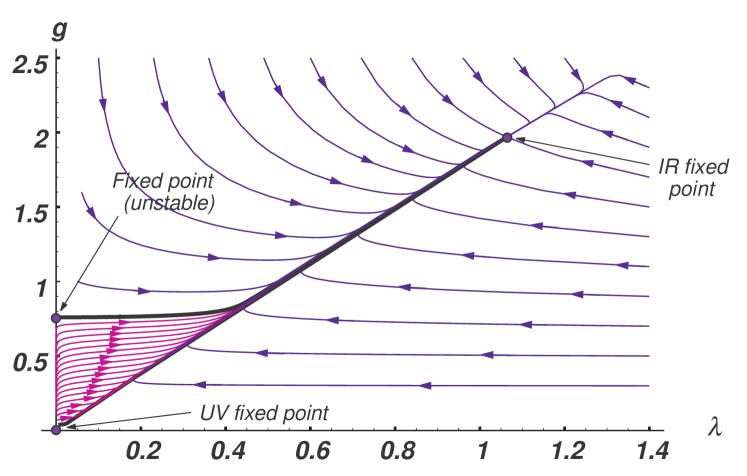
Figure 1: The renormalization-group infrared flow of the coupling constants $(\lambda,g)$ in the magnetic SQCD, for $\tilde{N_{c}}=7$, $N_{f}=20$. The infrared and ultraviolet fixed points value are indicated. All initial values shown in the plot flow to the infrared fixed-point couplings. The region bounded by the thick line is asymptotically free; strictly speaking, the theory exists only within this region.

3 Gauging Global Symmetries

Scale-invariant theories do not admit particle interpretation for their conformal fields unless their conformal dimensions are those of free fields. Even though Seiberg duality states that the electric theory gives precisely the same physics as the magnetic theory in the infrared limit, it is still not clear to the authors what physical quantities can be compared between these superconformal theories. The challenge is to identify suitable physical quantities of interest and to develop techniques to calculate them exactly in the infrared limit. Unlike in two-dimensional space-time, techniques are not well developed to work out correlation functions of conformal fields in four dimensions (see, however, [9]).

Historically, the study of the non-trivial gauge dynamics of QCD was done very effectively with $e^{+}e^{-}$ experiments. Here, a global symmetry ($U(1)_{EM}$) of QCD is gauged weakly and the gauge boson (photon) is produced off-shell from the $e^{+}e^{-}$ annihilation to create excitations in QCD. We would like to follow this program to gain more insight into the scale-invariant theories and especially their equivalence.

We first study the gauging of $U(1)_{B}$ in SQCD, and introduce “electrons” which are charged under $U(1)_{B}$ but not under the SQCD gauge group. We would then like to calculate the total cross section of creating excitations in SQCD from “electron-positron” annihilation.

At first sight, the cross sections do not appear to be the same in the electric and magnetic theories. At the tree-level, one can easily compute the Drell ratio $R$ (cross sections normalized by the “point” cross section $\sigma(e^{+}e^{-}\rightarrow\mu^{+}\mu^{-})$ where both “electron” and “muon” carry $U(1)_{B}$ charge unity). One finds

$$R\equiv\frac{\sigma(e^{+}e^{-}\rightarrow Q\bar{Q})}{\sigma(e^{+}e^{-}\rightarrow\mu^{+}\mu^{-})}=2N_{c}N_{f}$$ (19)

in the electric theory, while

$$R\equiv\frac{\sigma(e^{+}e^{-}\rightarrow q\bar{q})}{\sigma(e^{+}e^{-}\rightarrow\mu^{+}\mu^{-})}=2\tilde{N}_{c}N_{f}\left(\frac{N_{c}}{\tilde{N}_{c}}\right)^{2}=2N_{c}N_{f}\frac{N_{c}}{N_{f}-N_{c}}$$ (20)

in the magnetic theory. They clearly do not agree. Of course, this is only a tree-level result and receives corrections at all orders in perturbation theory. These results are only valid in the ultraviolet limit, where asymptotic freedom allows the approximation of $R$ by its tree-level value. In the infrared limit, if the two theories describe the same physics, the Drell ratios must agree after corrections from all orders in perturbation theory are included. The challenge is to find a way to calculate $R$ in both theories exactly in the infrared limit and compare them. We describe such technique below. A similar technique was employed by Anselmi et al [9] in the context of superconformal field theory.

The trick is to employ the NSVZ beta function for the running of the $U(1)_{B}$ coupling constant, and read off the vacuum polarization function from the beta function. Since the NSVZ beta function sums up contributions from all orders in perturbation theory, the result on the vacuum polarization function also includes contributions from all orders. One caveat is that it depends on the anomalous dimensions $\gamma_{f}$ which usually needs to be calculated in perturbation theory. In the infrared limit, however, the anomalous dimension factors for SQCD are known exactly, as discussed in the previous section, and one obtains the exact result for the vacuum polarization function. Then it can be analytically continued to time-like momenta and its cut yields the cross section.

In general, the running of a $U(1)$ coupling is given by

$$\frac{1}{e^{2}(\mu)}=\frac{1}{e^{2}(M)}+\Pi(M^{2})-\Pi(\mu^{2}),$$ (21)

where the vacuum polarization amplitude $\Pi(Q^{2})$ depends on the Euclidean momentum $Q^{2}=-q^{2}=-g_{\mu\nu}q^{\mu}q^{\nu}$ with the metric $(+1,-1,-1,-1)$. Comparing it to the NSVZ formula Eq. (2), we find

$$16\pi^{2}(\Pi(M^{2})-\Pi(\mu^{2}))=b_{0}\log\frac{\mu^{2}}{M^{2}}-2\sum_{f}T_{f}\log Z_{f}(\mu,M).$$ (22)

If the functional dependence of $Z_{f}$ on $\mu$ is known, the analytic continuation of the vacuum polarization function gives the $e^{+}e^{-}$ cross section:

$$R=16\pi^{2}\frac{1}{2\pi i}(\Pi(-s+i\epsilon)-\Pi(-s-i\epsilon)),$$ (23)

at the squared center-of-momentum energy $s$. We apply this technique to the electric and magnetic theories in the infrared limit.

The first step is to calculate the running of the $U(1)_{B}$ gauge coupling constant. We use the NSVZ formula with the infrared exact wave-function renormalization factors derived earlier (e.g. Eq. (3)). In the electric theory, we find

$$\frac{8\pi^{2}}{e^{2}(\mu)} = \frac{8\pi^{2}}{e^{2}(M)}-2N_{c}N_{f}\log\frac{\mu}{M}-2N_{c}N_{f}\log\left(\frac{\mu}{M}\right)^{(3N_{c}-N_{f})/N_{f}}$$ (24)

$$= \frac{8\pi^{2}}{e^{2}(M)}-6N_{c}^{2}\log\frac{\mu}{M}.$$

The same calculation can be done in the magnetic theory. The dual (anti) quarks carry baryon number $\pm N_{c}/\tilde{N}_{c}$, while the meson field has baryon number zero. The application of the NSVZ formula gives

$$\frac{8\pi^{2}}{e^{2}(\mu)}$$ (25)

$$= \frac{8\pi^{2}}{e^{2}(M)}-2\tilde{N}_{c}N_{f}\left(\frac{N_{c}}{\tilde{N}_{c}}\right)^{2}\log\frac{\mu}{M}-2\tilde{N}_{c}N_{f}\left(\frac{N_{c}}{\tilde{N}_{c}}\right)^{2}\log\left(\frac{\mu}{M}\right)^{(3\tilde{N}_{c}-N_{f})/N_{f}}$$

$$= \frac{8\pi^{2}}{e^{2}(M)}-6N_{c}^{2}\log\frac{\mu}{M}.$$

Therefore the running of the $U(1)_{B}$ coupling precisely agrees with what we obtained in the electric theory, despite quite distinct expressions at the intermediate stage of the calculations. This agreement makes the physical equivalence of the two theories much more direct and intuitive.

Using the definition of the vacuum polarization function (21), one finds

$$16\pi^{2}(\Pi(M^{2})-\Pi(\mu^{2}))=-6N_{c}^{2}\log\frac{\mu^{2}}{M^{2}}.$$ (26)

This is the exact result in the infrared limit $\mu^{2}\ll\Lambda^{2}$ where $\Lambda$ is the dynamical scale of the gauge theory. By analytically continuing $\Pi(\mu^{2})$ to the time-like region, the logarithm produces a cut, and one finds

$$R=6N_{c}^{2}$$ (27)

in the infrared limit ($s\ll\Lambda^{2}$). Because the running of the $U(1)_{B}$ coupling is precisely the same in the infrared limit for the electric and magnetic theories, this value of $R$ is also common for the two theories. This illustrates the equivalence of the two theories, at least in a limited fashion. It is amusing to note that the result does not depend on $N_{f}$ at all. From the point of view of electric theories, the result is the same for all values of $N_{f}$ from $\frac{3}{2}N_{c}$ to $3N_{c}$. On the other hand from the point of view of the magnetic theories, the result depends only on $N_{c}=N_{f}-\tilde{N}_{c}$. Another interesting point is that when the infrared fixed point coupling is perturbative, which happens when $N_{f}$ is close to but slightly less than $3N_{c}$ in the electric theory, the exact result (27) and the tree-level result in the electric theory (19) agree approximately. They agree exactly in the limit $N_{f}\rightarrow 3N_{c}-0$ as noted earlier. The same comment applies when $N_{f}$ is close to but slightly above $\frac{3}{2}N_{c}$; the exact result (27) and the tree-level result in the magnetic theory (20) agree approximately. They agree exactly in the limit $N_{f}\rightarrow\frac{3}{2}N_{c}+0$.

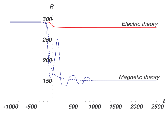
Figure 2: The behavior of the Drell $R$-ratio for the electric and magnetic SQCD as a function of $t=\log(\sqrt{s}/\Lambda)$, where $s$ is the center-of-momentum energy squared and $\Lambda=M\exp(-8\pi^{2}/g_{h}^{2}(M)b_{0})$. $M$ is the ultraviolet cut-off and $g_{h}$ is the holomorphic coupling. We chose $N_{c}=7$ and $N_{f}=20$ so that the electric theory is weakly-coupled for the entire $s$ range. The magnetic theory is strongly-coupled, and we cannot calculate $R$ for the interpolating region $s\sim\Lambda^{2}$. There are exact results for the limits $s\gg\Lambda^{2}$ and $s\ll\Lambda^{2}$, however. The dashed curves show two possible extreme behaviors in the interpolating region.

For illustrative purpose, in Fig. 2 the behavior of the $R$ is depicted as a function of $s$ in both the electric and magnetic theories for $N_{f}$ close to but slightly less than $3N_{c}$. In this case the electric theory is weakly coupled and one can estimate $R$ throughout the whole energy range from $s\ll\Lambda^{2}$ to $s\gg\Lambda^{2}$. We find:

$$R(s)=2N_{f}N_{c}\left(1+\frac{g^{2}(s)}{8\pi^{2}}2C_{2}+O(g^{4})\right),$$ (28)

where $C_{2}=(N_{c}^{2}-1)/2N_{c}$. This expression smoothly interpolates the infrared and ultraviolet limits (Eqs. (27) and (19)) given the fixed point coupling Eq. (8). The magnetic theory is strongly coupled; however we calculated $R$ in two extreme limits: $s\ll\Lambda^{2}$ and $s\gg\Lambda^{2}$. We do not know how the two extreme values are interpolated. Some possible behaviors are illustrated in the plot. One sees a few remarkable facts in this plot. First of all, the values of $R$ are the same in both theories in the low-energy limit, while they differ in the high-energy limit; this is precisely what is expected from the duality conjecture. Second, the $R$-values “drop” at the dynamical scale (this was observed, in a different context, by the authors of [9]). The effect is especially prominent in the strongly coupled side (the magnetic theory for the particular example in the plot). There is a plateau at the low-energy side, it goes through an interpolating region with either a smooth or wild behavior around the dynamical scale, and a new plateau sets in. The new plateau is lower than the other one. The behavior which interpolates two plateaus is reminiscent of a threshold in QCD, e.g., the $J/\psi$ region if it contains many bumps, or the $t\bar{t}$ threshold if it is smooth. However, thresholds in QCD always make the plateau higher. The behavior in the plot appears, therefore, “exotic”, i.e., contrary to common intuition. The drop is, of course, due to the decrease in the gauge coupling constant from the infrared fixed-point value to the asymptotically small coupling rather than the threshold effect of exciting new degrees of freedom.

The same analysis holds for the $SU(N_{f})$ non-Abelian gauge groups. The result in the electric theory is

$$\frac{8\pi^{2}}{e^{2}(\mu)}+N_{f}\log e^{2}(\mu)$$ (29)

$$= \frac{8\pi^{2}}{e^{2}(M)}+N_{f}\log e^{2}(M)+(3N_{f}-\frac{1}{2}N_{c})\log\frac{\mu}{M}-\frac{1}{2}N_{c}\log\left(\frac{\mu}{M}\right)^{\frac{(3N_{c}-N_{f})}{N_{f}}}$$

$$= \frac{8\pi^{2}}{e^{2}(M)}+N_{f}\log e^{2}(M)+\left(3N_{f}-\frac{1}{2}\frac{3N_{c}^{2}}{N_{f}}\right)\log\frac{\mu}{M}.$$

In the magnetic theory, the dual quarks as well as the meson fields contribute to the running. We find

$$\frac{8\pi^{2}}{e^{2}(\mu)}+N_{f}\log e^{2}(\mu)$$ (30)

$$= \frac{8\pi^{2}}{e^{2}(M)}+N_{f}\log e^{2}(M)+(3N_{f}-\frac{1}{2}\tilde{N}_{c}-\frac{1}{2}N_{f})\log\frac{\mu}{M}$$

$$-\frac{1}{2}\tilde{N}_{c}\log\left(\frac{\mu}{M}\right)^{(3\tilde{N}_{c}-N_{f})/N_{f}}-\frac{1}{2}N_{f}\log\left(\frac{\mu}{M}\right)^{-2(3\tilde{N}_{c}-N_{f})/N_{f}}$$

$$= \frac{8\pi^{2}}{e^{2}(M)}+N_{f}\log e^{2}(M)+\left(3N_{f}-\frac{1}{2}\frac{3N_{c}^{2}}{N_{f}}\right)\log\frac{\mu}{M}.$$

Similarly to the $U(1)_{B}$ case, the running of the coupling constants precisely agree.

One can introduce “leptons” coupled to the $SU(N_{f})$ gauge group, and discuss the “lepton anti-lepton annihilation” experiment. The cross sections agree between the electric and magnetic theories in the limit $s\rightarrow 0$. The second term in the bracket $\frac{1}{2}\frac{3N_{c}^{2}}{N_{f}}$ gives the “hadronic” cross section from “lepton anti-lepton” annihilation. Note that the first term $(3N_{f})$ is related to the production of “$W^{+}W^{-}$” from the $s$-channel “$W^{0}$-boson” and is irrelevant for our discussion. We do not go into further details in this letter.

4 Connection to Anomaly Matching

We have seen in the previous section that the running of the gauge coupling constants for gauged global symmetries in SQCD precisely agree in the infrared limit between the electric and magnetic theories for the entire $\frac{3}{2}N_{c}<N_{f}<3N_{c}$ range, where the theories are scale-invariant. This in turn guarantees that physical quantities, such as the $e^{+}e^{-}$ cross sections, are the same in the two theories. A natural question to address is whether the agreement of the cross sections poses a new constraint on duality or if it follows from conditions imposed in [1]. For the original arguments for duality to be sufficient, the agreement of the cross sections should not impose any new constraints but should follow from the conditions already imposed. We indeed find that the ‘t Hooft anomaly matching condition guarantees the agreement of the cross sections in these scale-invariant supersymmetric theories, and show why this is the case below. This was first pointed out, in a different context, in [9].

As discussed in the previous sections, the wave-function renormalization factors in scale-invariant theories are given by $Z_{f}(\mu,M)=(\mu/M)^{-3R_{f}+2}$ because of superconformal symmetry. First of all, it is interesting to check how the gauge coupling constant runs. Using the NSVZ formula,

$$\frac{8\pi^{2}}{g^{2}(\mu)}+C_{A}\log g^{2}(\mu)$$ (31)

$$= \frac{8\pi^{2}}{g^{2}(M)}+C_{A}\log g^{2}(M)+(3C_{A}-\sum_{f}T_{f})\log\frac{\mu}{M}-\sum_{f}T_{f}\log Z_{f}(\mu,M)$$

$$= \frac{8\pi^{2}}{g^{2}(M)}+C_{A}\log g^{2}(M)+3\left(C_{A}+\sum_{f}(R_{f}-1)T_{f}\right)\log\frac{\mu}{M}.$$

The condition that the gauge coupling constant does not run is then given by $(+1)C_{A}+\sum_{f}(R_{f}-1)T_{F}=0$. This is the same condition as the requirement that $U(1)_{R}$ be anomaly free under the gauge group, because the $U(1)_{R}$ charge of the gaugino is $+1$, and the fermionic component of the matter super-multiplet $f$ has $R$-charge $R_{f}-1$.

Now we apply the same analysis to the gauged global symmetry. The NSVZ formula is precisely the same except that $g^{2}$ and the group theory factors $C_{A}$ and $T_{f}$ are now those of the gauged global symmetry. The condition that the gauge coupling constant runs in the same way translates to the condition that the combination $\sum_{f}(R_{f}-1)T_{f}$ is the same between electric and magnetic theories, and this is nothing but the anomaly matching condition for $(U(1)_{R}G^{2})$, where $G$ is the global symmetry. It is reassuring that the ‘t Hooft anomaly matching condition, checked in all proposed dualities, is enough to guarantee that physical observables, such as the cross sections discussed in the previous section, are the same in the infrared between the electric and magnetic theories in the superconformal window.

It is noteworthy that the ‘t Hooft anomaly matching condition is presumably not enough to guarantee the equivalence of the cross sections in two scale-invariant theories without supersymmetry, such as those proposed in [11]. In the absence of supersymmetry, there is no reason for any one of the $U(1)$ symmetries of the theory to be related to the conformal transformation. The combination $U(1)_{R}G^{2}$ was important in the supersymmetric theories because $U(1)_{R}$ is in the same multiplet as the dilation and hence is indeed related to the dilation anomaly (i.e., running coupling constant) of the $G$ coupling. In non-supersymmetric theories, it is quite possible that the check of ‘t Hooft anomaly matching is far from enough to guarantee that the two theories describe the same infrared physics. The agreement of the cross sections considered here should be checked as an independent requirement for duality.

5 Other Physical Observables

We have seen that one can gauge global symmetries in SQCD and compare the running of the couplings in the electric and magnetic theories. We could furthermore calculate the “$e^{+}e^{-}$” cross sections in the infrared exactly in both theories and check that they are indeed the same. Even though these examples made the physical equivalence of two theories more manifest and explicit, they are only a few out of an infinite number of physical observables. All of them must be the same in the infrared when comparing the electric and magnetic theories if these are indeed dual. It is also important to see if the agreement of all observables follows from the ‘t Hooft anomaly matching condition or other consistency checks already done in the literature. The problem is that there are only very limited known methods of calculating other physical observables in theories with scale-invariant dynamics in four dimensions, unlike in the two dimensional case.

For instance, one can try to calculate the “light-by-light scattering” cross sections of the $U(1)_{B}$ “photons,” induced by loops of quarks. The effective operator

$$C\int d^{4}\theta W_{\alpha}W^{\alpha}\bar{W}_{\dot{\alpha}}\bar{W}^{\dot{\alpha}}$$ (32)

can be defined with a suitable infrared cutoff $\mu_{IR}$. At the lowest order in perturbation theory, the coefficient $C$ is proportional to $2N_{f}N_{c}$ in the electric theory and $2N_{f}\tilde{N}_{c}(N_{c}/\tilde{N}_{c})^{4}$ in the magnetic theory; they are clearly different. There is, as of today, no known powerful technique which would allow one to work out such a coefficient exactly in superconformal theories.

In this section, we will develop a very simple argument that allows one to constrain the form of $C$ and other related physical quantities. The hope is that these coefficients will be calculated exactly using the machinery of superconformal field theories, similar to what was accomplished in [9]. By constraining the form of the exact answer, it might be possible to gain some insight towards performing these computations, and, hopefully, to decide if the anomaly matching condition is enough to explain the agreement of these physical observables.

The argument proceeds as follows: we have already mentioned that lowest-order perturbation theory agrees with the exact answer in the limit $N_{f}\rightarrow 3N_{c}-0$ for the electric theory and $N_{f}\rightarrow 3/2N_{c}+0$ for the magnetic theory. We will use these limits to constrain the exact result.

Returning to the total “$e^{+}e^{-}$” cross section, the exact answer must be $2N_{c}N_{f}=6N_{c}^{2}$ for $N_{f}\rightarrow 3N_{c}-0$ and $2\tilde{N_{c}}N_{f}(N_{c}/\tilde{N_{c}})^{2}=6N_{c}^{2}$ for $N_{f}\rightarrow 3/2N_{c}+0$. Further requiring that the exact answer be written in terms of the global anomalies of the theory (which are guaranteed to be the same by anomaly matching), an obvious candidate appears: $-3(U(1)_{R}U(1)_{B}^{2})=6N_{c}^{2}$.

This candidate also satisfies another important constraint: the answer has to be invariant under simultaneous rescaling of the $U(1)_{B}$ gauge coupling by $n$ and the charge assigned to individual fields by $1/n$, that is if $e\rightarrow ne$ and $q\rightarrow q/n$ physical results should remain the same. Note that $\sigma(\gamma\rightarrow hadrons)\propto e^{2}$ and the final answer must therefore include $U(1)_{B}$ charges squared in order to guarantee this invariance.

By this sort of argumentation one cannot say that the correct answer has been determined, but an acceptable candidate has certainly been found. The exact answer, which was derived from superconformal invariance and the NSVZ exact beta function, in fact agrees with the naive guess above.

We now turn to the amplitude of $\gamma\gamma\rightarrow\gamma\gamma$, and start from the same set of assumptions: (i) the theories yield the same coefficient in the infrared; (ii) the exact result must agree with the lowest order perturbation theory in the two $N_{f}$ limits above; (iii) these coefficients can be written in terms of the global anomalies of the theory; (iv) the coefficient must be proportional to the $U(1)_{B}$ charge to the fourth power. All global anomalies can be easily computed and they are [1]

$$(SU(N_{f})^{3}) = N_{c}d^{(3)}(N_{f}),$$ (33)

$$(SU(N_{f})^{2}U(1)_{R}) = -{N_{c}^{2}\over{N_{f}}}d^{(2)}(N_{f}),$$ (34)

$$(SU(N_{f})^{2}U(1)_{B}) = N_{c}d^{(2)}(N_{f}),$$ (35)

$$(U(1)_{R}) = -N_{c}^{2}-1,$$ (36)

$$(U(1)_{R}^{3}) = N_{c}^{2}-1-2{N_{c}^{4}\over{N_{f}^{2}}},$$ (37)

$$(U(1)_{B}^{2}U(1)_{R}) = -2N_{c}^{2},$$ (38)

where $d^{(2)}(N_{f})=1/2\delta^{ab}$ and $d^{(3)}(N_{f})={\rm{Tr}}(T^{a}\{T^{b},T^{c}\})=d^{abc}$ ($a,b,c$ are $SU(N_{f})$ indices, $T^{a}$ are $SU(N_{f})$ generators).

According to the assumptions above, a candidate for the exact result must be:

$$C \propto (U(1)_{B}^{2}U(1)_{R})^{2}f+$$ (39)

$$(SU(N_{f})^{2}U(1)_{B})^{4}g+$$

$$(SU(N_{f})^{2}U(1)_{B})^{2}(U(1)_{B}^{2}U(1)_{R})h,$$

where $f,g,h$ are arbitrary functions of

$$(SU(N_{f})^{3}),(SU(N_{f})^{2}U(1)_{R}),(U(1)_{R}),(U(1)_{R}^{3})$$

and

$$(SU(N_{f})^{2}U(1)_{B})^{2}/(U(1)_{B}^{2}U(1)_{R}).$$

These will be referred to as the “invariant anomalies”, because they are not sensitive to rescalings of the $U(1)_{B}$ charge assignments. Note that, in order to make sense out of the $SU(N_{f})$ anomalies, one has to sum over all $SU(N_{f})$ indices.

Finally, conditions on $f$, $g$ and $h$ have to imposed such that

$$C(N_{f}=3N_{c})\propto 6N_{c}^{2}$$

and

$$C(N_{f}=3/2N_{c})\propto 24N_{c}^{2},$$ (40)

for any value of $N_{c}$, according to assumption (ii). There is no linear combination of integer products of the invariant anomalies that can meet these conditions. There are, of course, less “obvious” candidates.

Note that exact infrared results, whatever they might be, are functions exclusively of $N_{c}$ and $N_{f}$ (there are no other independent parameters in the theories), and it is always possible to write $N_{c}$ and $N_{f}$ in terms of a group of anomalies. One can, for example, take the $(U(1)_{R})$ and the $(SU(N_{f})^{2}U(1)_{B})^{2}/(U(1)_{B}^{2}U(1)_{R})$ anomalies and simply solve for $N_{c}$ and $N_{f}$:

$$N_{c} = \sqrt{-(U(1)_{R})-1},$$

$$N_{f} = \sqrt{1-8(SU(N_{f})^{2}U(1)_{B})^{2}/(U(1)_{B}^{2}U(1)_{R})}.$$ (41)

Having done that, it is easy to come up with a (simple) function of $N_{f}$ and $N_{c}$ that satisfies the conditions Eqs. (40). $54N_{c}^{4}/N_{f}^{2}$ clearly does the job, and a candidate for the exact answer that satisfies the conditions imposed above is

$$C\propto\frac{27}{2}{(U(1)_{B}^{2}U(1)_{R})^{2}\over{1-8(SU(N_{f})^{2}U(1)_{B})^{2}/(U(1)_{B}^{2}U(1)_{R})}},$$ (42)

where we used Eq. (5).

Next we address, within the same spirit, the “$W_{L}W_{L}\rightarrow W_{L}W_{L}$” scattering amplitude generated via quark loops. The subscript $L$ refers to the $SU(N_{f})$ group under which $Q$ and $q$ transform ($\tilde{Q}$ and $\tilde{q}$ transform under $SU(N_{f})_{R}$). Note that the coefficient of the amplitude is proportional to ${\rm{Tr}}(\{T^{a},T^{b}\}\{T^{c},T^{d}\})$ ($T^{a}$ are $SU(N_{f})$ generators), which can be written in terms of the $SU(N_{f})$ tensors present in the anomalies, namely $\delta^{ab}$ and $d^{abc}$. A candidate for the exact coefficient is

$$C_{W_{L}W_{L}W_{L}W_{L}}\propto{\rm{Tr}}(\{T^{a},T^{b}\}\{T^{c},T^{d}\})\frac{N_{c}^{2}}{N_{f}}=\left(d^{abe}d^{cde}+\frac{1}{2N_{f}}\delta^{ab}\delta^{cd}\right)\frac{N_{c}^{2}}{N_{f}}.$$ (43)

The expression above can easily be written in terms of the anomalies with the help of Eqs. (5) and the fact that

$$\frac{\delta^{ab}}{2N_{f}} = \frac{-(SU(N_{f})^{2}U(1)_{R})^{ab}}{N_{c}^{2}}=\frac{-(SU(N_{f})^{2}U(1)_{R})^{ab}}{-(U(1)_{R})-1},$$

$$d^{abc} = \frac{(SU(N_{f})^{3})^{abc}}{N_{c}}=\frac{(SU(N_{f})^{3})^{abc}}{\sqrt{-(U(1)_{R})-1}}.$$ (44)

Note that the expression for $C_{W_{L}W_{L}W_{L}W_{L}}$ in terms of anomalies only is highly non-trivial and involves, for example, inverse square-roots of polynomials of anomalies.

As one last example, we mention $W_{L}W_{L}\rightarrow W_{R}W_{R}$ scattering. The amplitude for this process must vanish at $N_{f}=3N_{c}-0$ and be proportional to $N_{f}$ (remember that for the magnetic theory there are the meson fields that transform under both $SU(N_{f})$ flavor groups) at $N_{f}=3/2N_{c}+0$. Therefore the candidate for the exact result cannot be a ratio of $N_{c}$ and $N_{f}$ to arbitrary powers (as in the previous cases), but has to be, for example, proportional to $3N_{c}-N_{f}$. We do not write the candidate in terms of anomalies, but it is clearly possible.

Note that, since it was shown that any function of $N_{c}$ and $N_{f}$ can be reexpressed in terms of anomalies (as, for example, in Eqs. (5)), it is always possible to write exact infrared results in terms of anomalies. It is, however, unclear whether the agreement between the electric and magnetic theories is guaranteed by the anomaly matching condition. Given the expressions outlined above, it is at best nonintuitive that future superconformal field theory exact computations will yield highly non-trivial functions of the anomalies as their results, especially because the candidates are very simple functions of $N_{c}$ and $N_{f}$. The situation outlined above should be contrasted to the “$e^{+}e^{-}$” total cross sections, described in the previous two sections.

Finally, it is clear that the “candidates” pointed out above are by no means guaranteed to be the exact answer. They agree with the exact answer in the limit when either the electric or the magnetic theory is arbitrarily weak ($N_{f}=3N_{c}-0,N_{f}=3/2N_{c}+0$), but other functions of $N_{c}$ and $N_{f}$ also have the same property. More constraints can be imposed on our candidates if one tries to analyze the superconformal theories when they are perturbative throughout the entire energy range ($N_{f}(1+\epsilon)=3N_{c}$ for the electric theory). In this case, next order in perturbation theory can be used and, because $g^{2}$ and $\epsilon$ are related in the infrared (see e.g. Eq.(8)), one can compare the order $g^{2}$ 1-loop correction to the order $\epsilon$ correction obtained from the candidate exact result. Note that this is indeed the case for the perturbative expression for $R$, Eq. (28).

Such a highly non-trivial check would be a very strong indication that one has indeed found the exact infrared answer for a given observable. We do not perform the next-order (2-loop) calculation for the amplitudes discussed above; it goes beyond the scope of our letter.

In summary, we hope we have raised and addressed in a limited fashion the following question: are all (or some) physical observables in superconformal field theories (in four dimensions) related to anomalies? If this indeed turns out to be the case, anomaly matching would be enough to guarantee the physical equivalence of two superconformal theories, which would shed light towards a “physical” understanding of Seiberg’s dualtity statements. On the other hand, if it is proven that there are physical observables which are not related to anomalies, then their exact computation would prove to be an extra duality condition.

6 Conclusion

In this letter we tried to verify that Seiberg’s duality conjecture is indeed correct. Such a check is at best non-trivial, given that one would have to perform computations in (very) strongly coupled theories.

To bypass this problem we have concentrated on the non-Abelian Coulomb phase, where both theories are superconformal and there is hope that some exact results can be obtained. The first challenge in this phase is to come up with appropriate physical observables that can be readily compared in both the electric and magnetic theories, especially because conformal theories do not, in general, allow any particle interpretation.

We have described total cross sections, related to the process of gauging the global symmetries of the theories, that can be used to check the duality conjecture. Some exact results were obtained and they agree between the magnetic and the electric theories.

Next we checked if the equality of these total cross sections poses any new duality conditions. For SQCD the anomaly matching condition is enough to guarantee that the total cross sections mentioned above are the same, thanks to superconformal invariance. We pointed out that the situation is different in non-supersymmetric dualities, and that the equalities of such cross sections should be included as an extra constraint.

Finally we analyzed other physical observables and tried to determine if their agreement between the electric and magnetic theories could also be explained by the anomaly matching condition. We found that that the functional form of the candidate exact result is highly non-trivial when expressed in terms of the global anomalies of the theories. It is not clear that superconformal field theory computations would yield such results.

It is, therefore, possible that the exact results do not have any relation to the global anomalies of the theory, and the fact that all physical processes agree for both theories is not guaranteed by Seiberg’s criteria alone.

More work is clearly required to fully understand this issue.

References

- [1] N. Seiberg, Nucl. Phys. B435, 129 (1995), hep-th/9411149.
- [2] I. Kogan, M. Shifman and A. Vainshtein, Phys. Rev. D53, 4526 (1996), hep-th/9507170.
- [3] D.R.T. Jones, Phys. Lett. 123B, 45 (1983).
- [4] V.A. Novikov, M.A. Shifman, A.I. Vainshtein, and V.I. Zakharov, Nucl. Phys. B229, 381 (1983).
- [5] V.A. Novikov, M.A. Shifman, A.I. Vainshtein, V.I. Zakharov, Nucl. Phys. B260, 157 (1985).
- [6] N. Arkani-Hamed and H. Murayama, hep-th/9707133.
- [7] M. Graesser and B. Morariu, Phys. Lett. B429, 313 (1998), hep-th/9711054.
- [8] T. Banks and A. Zaks, Nucl. Phys. B196, 189 (1982).
- [9] D. Alselmi et al, Nucl. Phys. B526, 543 (1998), hep-th/9708042.
- [10] M. E. Peskin and D. V. Schroeder, “An Introduction to Quantum Field Theory,” Reading, Addison-Wesley (1995), Chapter 18.
- [11] J. Terning, Phys. Rev. Lett. 80, 2517 (1998), hep-th/9706074.