hep-th/9810010 UCSD-PTH-98-34 September 1998

On the One Loop Fayet-Iliopoulos Term in

Chiral Four Dimensional Type I Orbifolds

Erich Poppitz

epoppitz@ucsd.edu

Department of Physics
University of California at San Diego
9500 Gilman Drive
La Jolla, CA 92093, USA

Abstract

We consider the generation of Fayet-Iliopoulos terms at one string loop in some recently found $N=1$ open string orbifolds with anomalous $U(1)$ factors with nonvanishing trace of the charge. Low-energy field theory arguments lead one to expect a one loop quadratically divergent Fayet-Iliopoulos term. We show that a one loop Fayet-Iliopoulos term is not generated, due to a cancellation between contributions of worldsheets of different topology. The vanishing of the one loop Fayet-Iliopoulos term in open string compactifications is related to the cancellation of twisted Ramond-Ramond tadpoles.

1. Introduction

The choice of ground state of string theory is one of the greatest obstacles to its phenomenological application. The breaking of spacetime supersymmetry and stabilization of the moduli remain two of the most pressing problems in this regard [1]. Most of the studies of supersymmetry breaking in the framework of string theory in the past have been in closed (heterotic) string compactifications. In recent years, however, it has been realized that the previously known five distinct string theories are related by various dualities. In particular, open string (type I) theories were found to be dual to closed string (heterotic) theories [2]. In view of the newly found dualities, it is natural to ask whether the weakly coupled description of the world might be in terms of one of the other, dual string theories. It is, therefore, of interest to investigate compactifications of type I theories and study their properties as well.

The first four dimensional type I orbifold with $N=1$ supersymmetry and chiral matter content was found in [3]. Since then, following [4], [5], a number of other examples have been constructed [6]. The occurrence of anomalous $U(1)$ factors of the gauge group is common in these examples. The anomaly is cancelled, as in the closed string case, by a generalized Green-Schwarz mechanism, but there are important differences [7], [8], [9]; see the discussion at the end of the Introduction and in the concluding Section.

It is well known that $N=1$ supersymmetry in four dimensions allows for Fayet-Iliopoulos (FI) terms for the $U(1)$ factors of the gauge group in the lagrangian, of the form:

$${\cal{L}}_{FI}~{}=~{}\zeta_{FI}^{2}~{}\int d^{4}\theta~{}V~{}.$$ (1.1)

FI terms can also play an important role in supersymmetry breaking [10], [11]. Moreover, in the case of anomalous $U(1)$ factors with nonvanishing trace of the charge, ${\rm Tr}~{}Q_{U(1)}\neq 0$, a FI term can be generated at one loop (a nonrenormalization theorem forbids the appearance of higher loop corrections [12], [13], [14]). The one loop contribution to the FI term is quadratically divergent, $\zeta_{FI}^{2}\sim\Lambda_{UV}^{2}{\rm Tr}~{}Q_{U(1)}$, and is therefore highly cutoff and regularization dependent; for example, it vanishes in dimensional regularization. It does, therefore, represent a “matching” contribution, and should be calculated in the underlying theory, valid beyond the scale of the ultraviolet cutoff, $\Lambda_{UV}$.

Anomalous $U(1)$ factors with Tr $Q_{U(1)}\neq 0$ also appear in closed string compactifications [13]. It is a well established fact, that at one closed string loop level a FI term is always generated [15], [16], [17], [18]. The torus amplitude leads to a finite contribution to the FI term, with the ultraviolet cutoff replaced by the inverse string scale, $\Lambda_{UV}\sim 1/\sqrt{\alpha^{\prime}}$.

Here we will investigate the generation of one loop FI terms in open string compactifications. An indication that the open string case might differ from the closed one is provided by considering the way the quadratic divergence is regulated in string theory graphs. The one loop FI term in field theory is proportional to $\int d^{4}p/p^{2}$, and represents a quadratically divergent contribution. In string theory, it is replaced by

$$\int~{}{d^{4}p\over p^{2}}\rightarrow\int~{}d^{4}p~{}\int_{t_{min}}^{\infty}~{}dt~{}e^{-tp^{2}}~{},$$ (1.2)

where $t$ denotes the modulus of the relevant worldsheet.

In the closed string case, $t\sim{\rm Im}~{}\tau$, where $\tau$ is the modular parameter of the torus. Since each torus is counted only once (due to modular invariance), the integration over $\tau$ is restricted to the fundamental region $|\tau|\geq 1$, ${\rm Im}~{}\tau>0$, $|{\rm Re}~{}\tau|\leq 1/2$; hence the lower limit of integration in (1.2) never vanishes, $t_{min}>0$. This implies that momenta of order the inverse string scale and higher are always cut off from the momentum integral (all scales in (1.2) are in terms of the string scale, $\alpha^{\prime}$, which we set, hereafter, equal to $1/2$).

In the case of the open string, $t$ also represents the modulus of the relevant worldsheet—the cylinder or Möbius strip. Since there is no modular invariance, the lower limit of the modulus integral in (1.2) is zero, $t_{min}=0$. Therefore the high loop-momentum contributions are not cut off and the divergent parts must cancel between different graphs (since we believe that string theory is finite).

In the rest of the paper, we will show that this cancellation does, in fact, occur. We perform the one loop open string calculation of the FI term in a type I compactification in the orbifold limit. We will concentrate on the simplest case, the $T^{6}/Z_{3}$ orbifold of type I theory [3]. We will show that the contributions of the cylinder and Möbius strip cancel exactly. Therefore, there is no FI term generated at the one loop level. We will see that the vanishing of the one loop FI term is closely related to the cancellation of twisted Ramond-Ramond tadpoles, which is important for consistency of the orbifold [5].

Our main conclusion is that the only contribution to the FI term in the open string compactifications considered here occurs at tree-level and is due to giving expectation values to the orbifold blow-up modes (these contributions have been discussed first in [7] and recently in [9]). Since the FI term now is due to the expectation value of a modulus, its value is, at least in perturbation theory, arbitrary, rather than the fixed value (of order the string scale) obtained in the heterotic case. In the final section of the paper, we consider these tree-level contributions in some more detail and point out some implications for supersymmetry breaking. We believe, based on the heuristic arguments given above, that our result is more generally valid; we leave its extension to other type I compactifications for future work.

2. The calculation

2.1 The $Z_{3}$ orbifold of type I theory

In this section, we will describe in some detail the orbifold, introduce our notation, and find explicitly the Chan-Paton factors of the massless open string modes that survive the orbifold projection. These will be useful in the calculation of the subsequent sections and in the interpretation of the results.

The $Z_{3}$ orbifold of type I theory was first constructed in ref. [3]. We will describe the construction in the more familiar language of ref. [5]. To describe the orbifold, and further in our calculation, we use light-cone variables $X^{\pm}=(X^{0}\pm X^{9})/\sqrt{2}$. The compact directions (the six-torus $T^{6}$) are $X^{1},\ldots,X^{6}$. To construct the $Z_{3}$ orbifold of type I theory, one mods out the Hilbert space of type I theory by the action of a $Z_{3}$ discrete symmetry. We take the operator

$$\hat{\alpha}~{}=~{}\exp\left\{-~{}{4\pi i\over 3}\left(\hat{J}_{12}~{}+~{}\hat{J}_{34}~{}+~{}\hat{J}_{56}\right)\right\}~{}$$ (2.1)

to generate the $Z_{3}$ symmetry. Here $\hat{J}_{ij}$ are the generators of rotations in the $ij$-plane ($i,j=1,\ldots,8$). Note that, with this definition, $\hat{\alpha}^{3}=1$ in the spinor representations as well. We will employ the unhatted letter $\alpha$ to denote $e^{2\pi i/3}$. The transverse (to the light-cone) noncompact directions are $X^{7}$ and $X^{8}$. The orbifold action (2.1) leaves invariant four supercharges ($N=1$ in four dimensions).

The construction of the closed string sector of the orbifold proceeds by projecting out closed string states that are not invariant under the action of $\hat{\alpha}$; in addition, one has to add twisted sectors. This results in the appearance of 27 chiral multiplets in the twisted sector of the orbifold (one chiral multiplet for each of the $3^{3}=27$ fixed points) [3]. The construction of the open string sector of the orbifold proceeds along the lines of [7], [5]. One finds that the orbifold group also acts on the Chan-Paton factors $\lambda$, as

$$\hat{\alpha}:~{}\lambda\rightarrow\gamma_{\alpha}\lambda\gamma_{\alpha}^{-1}~{}.$$ (2.2)

Here $\gamma_{\alpha}$ is an embedding of the orbifold group in the gauge group, whose explicit form we will give below. $\gamma_{\alpha}$ has to satisfy the tadpole cancellation conditions [5], which, in this case, amount to requiring Tr $\gamma_{\alpha}=-4$.

The massless open string states that survive the orbifold projection can be found by considering the action of the orbifold group on the massless vertex operators. The massless boson open string vertex operator in type I theory is (we use light-cone gauge and Green-Schwarz fermions; our notations are identical to those of [1]):

$$V(\xi,k;w)~{}=~{}\xi^{i}~{}\left(\dot{X}^{i}-R^{ij}(w)~{}k^{j}\right)~{}e^{ik\cdot X(w)}~{}{\hat{\lambda}}~{},$$ (2.3)

where $R^{ij}(w)=(1/4)S^{a}(w)\gamma^{ij}_{ab}S^{b}(w)$, and $S^{a}$ are the Green-Schwarz fermions transfoming in the ${\bf 8_{c}}$ spinor representation of $SO(8)$ [1]. Here $\hat{\lambda}$ represents the relevant Chan-Paton factor. Gauge bosons in the four dimensional theory have polarization vectors, whose transvere components are along the $X^{7}$, $X^{8}$ directions, while the polarization vectors for scalars are along the $X^{1}\ldots X^{6}$ directions. We will take as an example

$$\xi_{1}~{}=~{}{1\over\sqrt{2}}~{}(0,~{}1,~{}-i,~{}0,\ldots,0)~{},~{}~{}\xi_{2}~{}=~{}~{}{1\over\sqrt{2}}~{}(0,~{}1,~{}i,~{}0,\ldots,0)~{},$$ (2.4)

where $\xi_{1}$ and $\xi_{2}$ correspond to a complex scalar ($\xi_{2}$) and its complex conjugate ($\xi_{1}$); the components of the polarization vectors are listed in order $X^{0},X^{1},...,X^{9}$.

The massless open string spectrum is now found by requiring that the massless state vertex operators be invariant under the combined action of $\hat{\alpha}$ (2.1) on the fields in (2.3) and on the Chan-Paton factor $\hat{\lambda}$ (2.2). Using the tadpole cancellation condition to determine the form of $\gamma_{\alpha}$, one finds that the Chan-Paton factors of the states invariant under the orbifold projection are as described explicitly below.

We use a basis where the $SO(32)$ Chan-Paton factors are real antisymmetric matrices. The action of the orbifold group on the Chan-Paton factors (see eq. (2.2)), is represented by the $SO(32)$ matrix:

$$\gamma_{\alpha}~{}=~{}\left(\begin{array}[]{ccc}{\bf 1}_{8}&0&0\\ 0&-{1\over 2}~{}{\bf 1}_{12}&{\sqrt{3}\over 2}~{}{\bf 1}_{12}\\ 0&-{\sqrt{3}\over 2}~{}{\bf 1}_{12}&-{1\over 2}~{}{\bf 1}_{12}\end{array}\right)~{},$$ (2.8)

obeying the tadpole consistency condition Tr $\gamma_{\alpha}=-4$. Here we use a block-matrix notation: ${\bf 1}_{k}$ denotes a ($k\times k$) dimensional unit matrix.

To find the gauge fields’ Chan-Paton factors, we note that vertex operators with polarization vectors along the noncompact directions are invariant under the action of $\hat{\alpha}$. Hence the gauge Chan-Paton factors should obey $\lambda=\gamma_{\alpha}\lambda\gamma_{\alpha}^{-1}$. Thus, we find

$$\lambda_{gauge}~{}=~{}\left(\begin{array}[]{ccc}{\bf A}^{\prime}&0&0\\ 0&{\bf A}&{\bf S}\\ 0&-{\bf S}&{\bf A}\end{array}\right)~{},$$ (2.12)

where ${\bf A}^{\prime}$ is an ($8\times 8$) antisymmetric matrix that generates $SO(8)$, while ${\bf A}$ and ${\bf S}$ are ($12\times 12$) antisymmetric and symmetric matrices, respectively. ${\bf A}$ and ${\bf S}$ together generate $U(12)$, so that ${\bf A}-i{\bf S}$, ${\bf A}+i{\bf S}$ are the antihermitean generators of the fundamental and antifundamental representations, respectively. For further use, note that the anomalous $U(1)$ factor is generated by the trace part of the symmetric tensor. From eq. (2.12) it follows that the gauge group of the four dimensional theory is $SO(8)\times U(12)$.

The Chan-Paton factors for the matter fields are complex antisymmetric matrices (recall that the matter fields are complex linear combinations of gauge bosons polarized in the compact directions; see eqs. (2.3, 2.4)). Since under the action of $\hat{\alpha}$, the field dependent part of the scalar vertex operator (denoted by $V^{\prime}$) with polarization vector $\xi_{1}$, see eq. (2.4), transforms as $\hat{\alpha}V^{\prime}\hat{\alpha}^{-1}=\alpha^{-1}V^{\prime}$, in order for the state to be invariant, its Chan-Paton factor $\lambda^{\dagger}$ has to satisfy $\gamma_{\alpha}\lambda^{\dagger}\gamma_{\alpha}^{-1}=\alpha\lambda^{\dagger}$, and is explicitly given by:

$$\lambda_{matter}^{\dagger}~{}=~{}\left(\begin{array}[]{ccc}0&{\bf b}&i~{}{\bf b}\\ -{\bf b}^{T}&{\bf a}&-i~{}{\bf a}\\ -i~{}{\bf b}^{T}&-i~{}{\bf a}&-{\bf a}\end{array}\right)~{}.$$ (2.16)

Here we use the same block structure as in (2.12): ${\bf b}$ is an ($8\times 12$) dimensional matrix, representing the fields that transform under both $SO(8)$ and $U(12)$, while ${\bf a}$ is an ($12\times 12$) antisymmetric tensor. The complex conjugate matter fields are represented by the hermitean conjugate matrix $\lambda_{matter}$. It is easy to check that under gauge transformations, $\delta\lambda_{matter}^{\dagger}=\left[\lambda_{gauge},\lambda_{matter}^{\dagger}\right]$, the factors ${\bf b}$ and ${\bf a}$ transform (in terms of finite transformations of $SO(8)$, ${\bf O}=e^{{\bf A}^{\prime}}$, and $U(12)$, ${\bf U}=e^{{\bf A}-i{\bf S}}$) as: ${\bf a}\rightarrow{\bf Ua}{\bf U}^{T}$, ${\bf b}\rightarrow{\bf Ob}{\bf U}^{\dagger}$. Thus, the massless matter content of the orbifold in terms of chiral superfields is given by three copies of $(\raisebox{-0.5pt}{\hbox{\rule{0.4pt}{6.5pt}\hskip-0.4pt\rule{6.5pt}{0.4pt}\hskip-6.5pt\rule[6.5pt]{6.5pt}{0.4pt}}\rule[6.5pt]{0.4pt}{0.4pt}\hskip-0.4pt\rule{0.4pt}{6.5pt}},\overline{\raisebox{-0.5pt}{\hbox{\rule{0.4pt}{6.5pt}\hskip-0.4pt\rule{6.5pt}{0.4pt}\hskip-6.5pt\rule[6.5pt]{6.5pt}{0.4pt}}\rule[6.5pt]{0.4pt}{0.4pt}\hskip-0.4pt\rule{0.4pt}{6.5pt}}})+({\bf 1},\raisebox{-3.5pt}{\hbox{\rule{0.4pt}{6.5pt}\hskip-0.4pt\rule{6.5pt}{0.4pt}\hskip-6.5pt\rule[6.5pt]{6.5pt}{0.4pt}}\rule[6.5pt]{0.4pt}{0.4pt}\hskip-0.4pt\rule{0.4pt}{6.5pt}}\hskip-6.9pt\raisebox{3.0pt}{\hbox{\rule{0.4pt}{6.5pt}\hskip-0.4pt\rule{6.5pt}{0.4pt}\hskip-6.5pt\rule[6.5pt]{6.5pt}{0.4pt}}\rule[6.5pt]{0.4pt}{0.4pt}\hskip-0.4pt\rule{0.4pt}{6.5pt}})$ under $SO(8)\times U(12)$, corresponding to the three complex compact directions. The $U(1)$ charges of the fields ${\bf a}$ and ${\bf b}$ are $2$ and $-1$, respectively.

It is easily seen, then, that the $U(1)$ is anomalous, and that Tr $Q_{U(1)}\neq 0$. Thus, low-energy field theory considerations [11, 12, 13, 14] lead one to expect a one loop quadratically divergent FI term. The following sections are devoted to the string calculation of this term.

2.2 Factorization of the four-point amplitude

In this section, we will describe the idea behind the calculation of the one loop FI term in string theory. The main points below are as in the closed string calculation; we will be correspondingly brief and only mention the essential differences.

Adding a FI term (1.1) to the lagrangian leads to scalar masses—restoring the canonical normalization of the vector superfield kinetic term and expanding the anomalous $U(1)$ D-term potential, see [10], one finds mass terms for all scalar fields, proportional to their $U(1)$ charges: $m^{2}_{\phi}\sim g^{2}q_{\phi}\zeta_{FI}^{2}$. It is these mass terms that are easiest to compute in string theory [13], [15], [16], [18].

Figure 1: Factorization of the four-point amplitude of gauge boson$-$scalar (scalars are denoted by a dashed line) scattering in the $s$-channel ($s=-(k_{1}+k_{2})^{2}=-2k_{1}\cdot k_{2}$); $x$ and $w$ denote the points the vertex operators are attached to the world sheet (2.17). A summation over the four noncyclic permutations, which allow for $s$-channel poles, accounts for the correct Chan-Paton factor of the state exchanged in the $s$-channel.

Since string amplitudes are on-shell quantities, it is natural to define masses as poles in scattering amplitudes at appropriate values of the external momenta. To compute the one loop contribution to the scalar masses in our orbifold, consider the elastic scattering amplitude of a $U(1)$ gauge boson and a scalar (see Fig.1). Let $k_{1}$ and $k_{2}$ be the momenta of the incoming gauge boson and scalar, respectively, and $k_{3}$ and $k_{4}$—of the outgoing. One expects a pole in the amplitude at $s=m^{2}$, where $m$ is the mass of any scalar that can be produced in the $s$-channel. In other words, one expects $A\sim 1/(s-m^{2})\simeq m^{2}/s^{2}$; the second equality is true if $m$ is treated as a perturbation around zero tree-level mass (i.e. as a “mass insertion”). To see this factorization explicitly, consider the OPE of a scalar and gauge boson vertex operators:

$$V_{gauge}(\xi_{g},k_{1};x)~{}V_{scalar}(\xi_{m},k_{2};w)~{}=~{}(\xi_{g}\cdot k_{2})~{}\left({w\over x-w}\right)^{1-k_{1}\cdot k_{2}}~{}:V_{scalar}(\xi_{m},k_{1}+k_{2};w):~{}+~{}\ldots~{}.$$ (2.17)

The following identity is useful in deriving eq. (2.17), as well as eq. (2.21) from Sect. 2.3:

${1\over 2}~{}(a_{1}\cdot\gamma_{ab}\cdot b_{1})~{}(a_{2}\cdot\gamma_{bc}\cdot b_{2})-{1\over 2}~{}(a_{1}\cdot\gamma_{cb}\cdot b_{1})~{}(a_{2}\cdot\gamma_{ba}\cdot b_{2})~{}=~{}$

$$-(a_{1}\cdot b_{2})~{}(a_{2}\cdot\gamma_{ac}\cdot b_{1})+(b_{1}\cdot b_{2})~{}(a_{2}\cdot\gamma_{ac}\cdot a_{1})+(a_{1}\cdot a_{2})~{}(b_{2}\cdot\gamma_{ac}\cdot b_{1})-(b_{1}\cdot a_{2})~{}(b_{2}\cdot\gamma_{ac}\cdot a_{1})~{}.$$ (2.18)

The matrices $\gamma_{ab}^{ij}$ are as defined in [1]. In (2.17) $\xi_{g}$ ($\xi_{m}$) are the polarization vectors of the gauge boson (scalar) and the dots denote terms that do not contribute to the factorized amplitude in the $s\rightarrow 0$ limit. Inserting (2.17) into the four-point amplitude [1], and integrating over $x$, using

$${\rm lim}_{k_{1}\cdot k_{2}\rightarrow 0}~{}\int_{w}^{1}{dx\over x}~{}\left({w\over x-w}\right)^{1-k_{1}\cdot k_{2}}~{}F(x)~{}=~{}{1\over k_{1}\cdot k_{2}}~{}F(w)~{}+~{}{\rm nonsingular}~{},$$ (2.19)

one finds that the four-point amplitude in the limit $s\sim k_{1}\cdot k_{2}\rightarrow 0$ factorizes (as shown on Fig. 1; see also [15], [16]) into the product of a tree-level amplitude for producing a scalar (the $\xi_{g}\cdot k_{2}$ factor in (2.17)), a massless scalar propagator (the $1/k_{1}\cdot k_{2}$ factor due to (2.19)), a two point scalar amplitude, with the scalar vertex operators taken off-shell (as on the r.h.s. of eq. (2.17)), another massless scalar propagator, and another tree-level amplitude for producing a scalar; we note that factorization also holds for the surface with a crosscap.

From the above discussion, we conclude that the two-point scalar amplitude plays the role of mass insertion in field theory. The one loop correction to the mass is therefore found by computing the two-point scalar amplitude with the scalars taken slightly off-shell, and by taking the limit $k^{2}\rightarrow 0$ at the end of the calculation [15], [16].

2.3 Vanishing of the two-point scalar amplitude

As argued in the previous section, the scalar mass squared is related to the one loop scalar two-point function, computed slightly off-shell, with the on-shell limit taken in the end of the calculation. The computation of the scalar two-point function and the demonstration of its vanishing is the subject of this section. The two-point one-loop scalar amplitude is of the same order, ${\cal{O}}(g_{string})\sim g^{2}$, as the field theory one-loop contribution to the scalar mass: the annulus and Möbius strip have $\chi=0$, while each vertex operator contributes a factor of $g_{string}^{1/2}\sim g$.

To calculate the two-point scalar amplitude, we will use the operator formalism with Green-Schwarz fermions. The expression for the two-point function in type I theory has the form [1]:

$A(k_{1},k_{2})~{}=$

$$~{}\int_{0}^{1}{dw\over w}~{}\int_{w}^{1}{dx\over x}~{}\int{d^{10}p\over(2\pi)^{10}}~{}{\rm Tr}\left[~{}{1+\hat{\alpha}+\hat{\alpha}^{2}\over 3}~{}V_{1}(\xi_{1},k_{1};x)~{}{1+\hat{\Omega}\over 2}~{}V_{2}(\xi_{2},k_{2};w)~{}{1+\hat{\Omega}\over 2}~{}w^{\hat{L}_{0}}~{}\right]~{}.$$ (2.20)

Here $V(\xi,k;x)$ are the vertex operators for the scalars, see eqs. (2.3, 2.4); they include the Chan-Paton factors appropriate for the states under consideration—the matrices of the form (2.16), which we denote $\lambda_{1}^{\dagger}$ and $\lambda_{2}$ for $V_{1}$ and $V_{2}$ in (2.20), respectively.

The trace in eq. (2.20) is over all states in the Hilbert space of type I string theory. The operator $(1+\hat{\alpha}+\hat{\alpha}^{2})/3$ performs a projection on $Z_{3}$ invariant states. In the formalism we are using [1], the Hilbert space is a tensor product of three spaces: the space of zero modes, times the Fock space of $X^{i}$ and $S^{a}$ oscillators, times the space of Chan-Paton indices (all states are also labeled by the loop momentum, the trace over which is factored out in (2.20)). The various operators in (2.20) act on one, or on several, components of the tensor product, as discussed below. Thus, the trace in (2.20) reduces to a sum of products of traces in each of these spaces. The operator $\hat{L}_{0}\equiv{\hat{p}^{2}\over 2}+\hat{N}$, where $\hat{N}$ is the excitation number operator. Here $p$ is momentum of the string running in the loop. For a compact direction of radius $R$, we have to replace the continuum momentum integral in (2.20) by a sum over momentum modes: $\int dp\rightarrow(1/R)\sum_{n}$. $\hat{\Omega}=-(-)^{\hat{N}}$ is the orientation reversal operator. It is important for what follows that the operators $\hat{\alpha}$ and $\hat{\Omega}$ act on the Chan-Paton indices as well; we will include the overall minus sign in $\hat{\Omega}$ in its action on the Chan-Paton factors.

Because of the trace over the supersymmetric zero modes (denoted hereafter by ${\rm Tr}_{0}$), the terms proportional to $\dot{X}$ in the vertex operators (2.3) do not contribute to trace (using the formulas for zero-mode traces of [1], and the definition of $\hat{\alpha}$ (2.1), it is easy to see that ${\rm Tr}_{0}~{}\hat{\alpha}=0$). Hence, only the pieces involving the Green-Schwarz fermions in the vertex operators (2.3) contribute to the trace in (2.20). It is clear, then, that the amplitude will be proportional to $k_{1}\cdot k_{2}$. Now, because of momentum conservation $k_{1}=-k_{2}=k$; hence, in the limit when the two scalars are on shell, $k_{1}\cdot k_{2}=-k^{2}=0$, the two-point amplitude would naively vanish. However, as in the closed string case, the loop integral in (2.20) can contribute a $1/k^{2}$ factor, which cancels the overall $k^{2}$ factor and leads to a nonvanishing result as the two scalars are taken on-shell [15, 16, 18]. To see this, consider the OPE of two scalar vertex operators (see (2.18)):

$V_{scalar}(\xi_{1},k_{1};x)~{}V_{scalar}(\xi_{2},k_{2};w)~{}=~{}$

$$~{}{1\over 4}~{}(k_{1}\cdot k_{2})~{}\left({w\over x-w}\right)^{1-k_{1}\cdot k_{2}}~{}\xi_{1}^{i}~{}\gamma_{ab}^{ij}~{}\xi_{2}^{j}~{}S^{a}(w)~{}S^{b}(w)~{}:e^{i(k_{1}+k_{2})\cdot X(w)}:~{}+~{}\ldots~{},$$ (2.21)

where, as usual, the dots denote terms which do not contribute to the $1/k^{2}$ pole. Inserting (2.21) into (2.20) and integrating over $x$, eq. (2.19), we see that the $1/k^{2}$ factor cancels the overall $k^{2}$ factor in (2.21). Thus, the calculation of the nonzero contribution to the two point function reduces to:

$$A(k^{2}\rightarrow 0)~{}=~{}{\rm const.}~{}\int_{0}^{1}{dw\over w}\left({2\pi\over\log w}\right)^{2}~{}{\rm Tr}~{}\left({1+\hat{\alpha}+\hat{\alpha}^{2}\over 3}~{}R^{ij}(w)~{}{1+\hat{\Omega}\over 2}~{}w^{\hat{N}}\right)~{}\xi_{1}^{i}~{}\xi_{2}^{j}~{},$$ (2.22)

where we absorb various inessential factors in the overall constant, as mentioned below. In obtaining eq. (2.22), we have performed the $x$-integral as described above; see eq. (2.19). We have also performed the loop-momentum integral over the four noncompact momenta, resulting in the factor of $(2\pi/\log w)^{2}$. It is important to note, that since only the terms with $\hat{\alpha}$ and $\hat{\alpha}^{2}$ in (2.20) are nonvanishing (because of the zero-mode trace, as explained in the following paragraph), only vanishing momentum modes in the compact directions contribute to the trace (we have omitted the overall $1/(2\pi R)^{6}$ factor resulting from them, as well as the overall momentum conserving delta function).

Now we go on to the computation of the remaining trace in (2.22). We begin with considering the zero-mode traces. To this end, first note that the terms without insertions of $\hat{\alpha}$ do not contribute—the corresponding traces over the space of zero modes vanish, ${\rm Tr}_{0}R^{ij}_{0}=0$ (recall that one needs an insertion of at least eight zero modes to get nonvanishing zero-mode trace [1]). Here $R^{ij}_{0}=(1/4)S^{a}_{0}\gamma^{ij}_{ab}S^{b}_{0}$, where $S_{0}^{a}$ denote the zero modes of the Green-Schwarz fermions [1]. Furthermore, because of unbroken supersymmetry, it is also easy to see (as mentioned above) that ${\rm Tr}_{0}\hat{\alpha}=0$ ($\hat{\Omega}$ acts trivially on the zero modes). Therefore both fermion fields in (2.22) have to correspond to zero modes. Hence, the only zero-mode traces we need to compute are:

$${\rm Tr}_{0}~{}\hat{\alpha}~{}R^{12}_{0}~{}=~{}-3\sqrt{3}/2~{}~{}{\rm and}~{}~{}{\rm Tr}_{0}~{}\hat{\alpha}^{2}~{}R^{12}_{0}~{}=~{}3\sqrt{3}/2~{},$$ (2.23)

where, for brevity, we have only given the $R_{0}^{12}$ component, relevant for our choice of polarization vectors (2.4). The traces are computed using the formulae for the action of the rotation generators on the zero-mode states, given in [1], and the definition of $\hat{\alpha}$, eq. (2.1); we also note that, in view of our result, we only make use of the relative minus sign in (2.23), which can be obtained by computing the trace of the transposed matrix and using $(R^{ij}_{0})^{T}=-R^{ij}_{0}$, and $\alpha^{T}=\alpha^{2}$.

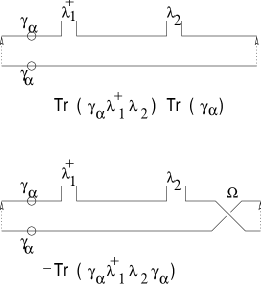
Figure 2: A schematic representation of the two worldsheets (the ends should be glued along the arrows), contributing to the $1/k^{2}$ pole in the scalar two point function. Insertions of $\gamma_{\alpha}$ are denoted by a circle. The Chan-Paton traces Tr ($\hat{\alpha}\hat{\lambda}_{1}^{\dagger}\hat{\lambda}_{2}$) and Tr ($\hat{\alpha}\hat{\lambda}_{1}^{\dagger}\hat{\lambda}_{2}\hat{\Omega}$) are computed by tracing the product of the matrices $\gamma_{\alpha}$ and $\lambda_{1,2}$ in the order they appear along each boundary of the worldsheet, and are shown under each worldsheet. A similar representation follows for the trace with $\hat{\alpha}\rightarrow\hat{\alpha}^{2}$ and amounts to replacing $\gamma_{\alpha}\rightarrow\gamma_{\alpha}^{-1}$. As explained in the text, because of the unbroken space-time supersymmetry, the term without insertions of $\hat{\alpha}$ in the trace does not contribute.

Now we go on to the traces over the Chan-Paton indices. We define the action of $\hat{\alpha}$ (and, similarly, of $\hat{\alpha}^{2}$) on the Chan-Paton indices, ${\hat{\alpha}}|ab\rangle=|cd\rangle(\gamma_{\alpha})_{ca}(\gamma_{\alpha})_{db}$, while the Chan-Paton factors from the vertex operators $\hat{\lambda}$ of (2.3) act on, say, the first indices only: ${\hat{\lambda}}|ab\rangle=|cb\rangle\lambda_{ca}$, since they are both attached to the same boundary; note that the above definition preserves the correct cyclic order, and is consistent with the action of $\hat{\alpha}$ on the Chan-Paton factors (2.2). For the evaluation of the Möbius strip, we also need the action of $\hat{\Omega}$ on the Chan-Paton indices: $\hat{\Omega}|ab\rangle=-|ba\rangle$, where, as mentioned above, we include the overall minus sign in the action on the Chan-Paton indices. Finally, $\langle cd|ab\rangle=\delta_{ca}\delta_{db}$. Thus, the Chan-Paton trace of the unit operator gives a factor of $n^{2}$ ($n$ being the number of $D$-branes), while the trace of $(1+\hat{\Omega})/2$ gives $(n^{2}-n)/2$ (with the above definition of $\hat{\Omega}$ appropriate for an $SO(n)$ projection; for us, $n=32$). In computing the various Chan-Paton traces, where appropriate, we also make use of $\gamma_{\alpha}^{T}=\gamma_{\alpha}^{-1}$, $\gamma_{\alpha}^{2}=\gamma_{\alpha}^{-1}$. The computation of the relevant—the ones with insertions of $\hat{\alpha}$ and $\hat{\alpha}^{2}$—Chan-Paton traces yields:

$${\rm Tr}_{C.-P.}\left(\hat{\alpha}~{}\hat{\lambda}_{1}^{\dagger}~{}\hat{\lambda}_{2}\right)~{} = ~{}{\rm Tr}\left(\gamma_{\alpha}~{}\lambda_{1}^{\dagger}~{}\lambda_{2}\right)~{}{\rm Tr}\left(\gamma_{\alpha}\right)~{}$$

$${\rm Tr}_{C.-P.}\left(\hat{\alpha}~{}\hat{\lambda}_{1}^{\dagger}~{}\hat{\lambda}_{2}~{}\hat{\Omega}\right)~{} = ~{}-~{}{\rm Tr}\left(\gamma_{\alpha}~{}\lambda_{1}^{\dagger}~{}\lambda_{2}~{}\gamma_{\alpha}\right)~{}.$$ (2.24)

Eq. (S0.Ex1) can be verified using the rules outlined above (which are also graphically represented on Fig. 2). Similar relations hold for the traces where $\hat{\alpha}$ is replaced by $\hat{\alpha}^{2}$—one simply replaces $\gamma_{\alpha}$ by its inverse in (S0.Ex1).

Finally, we consider the trace over all nonzero modes—the Fock space of $X^{i}$ and $S^{a}$ oscillators. It is easy see that these two traces precisely cancel, because of the unbroken space-time supersymmetry. For example, the trace over the $X^{i}$ oscillators, Tr $\hat{\alpha}~{}w^{\hat{N}}$, yields a factor of $\prod_{n=1}^{\infty}(1-\alpha~{}w^{n})^{3}(1-\alpha^{-1}~{}w^{n})^{3}(1-w^{n})^{2}$ in the denominator, while the trace over the fermionic nonzero modes yields the same factor in the numerator; similarly, the contribution of the $X^{i}$ oscillators to Tr $\hat{\alpha}~{}\hat{\Omega}~{}w^{\hat{N}}$ is precisely cancelled by the contribution of the $S^{a}$ oscillators. Thus, we conclude that no massive string excitations contribute to the two-point function, as in the closed string case, and in accord with field theory expectations.

Now we can assemble the contributions (2.23, S0.Ex1) to the two-point amplitude (2.22). We write the amplitude (2.22) as $A=A_{C}+A_{MS}$, omitting the overall constant. Note that the contributions of the Chan-Paton and zero-mode traces factorize and can be combined (below we use eq. (2.4) for $\xi_{1}$ and $\xi_{2}$). The cylinder contribution $A_{C}$ (the term without $\hat{\Omega}$ in (2.22)) to the two point amplitude is then, using (2.23, S0.Ex1):

$$A_{C}~{} = ~{}{\rm Tr}\left[\left(-i\gamma_{\alpha}+i\gamma_{\alpha}^{-1}\right)\lambda^{\dagger}_{1}\lambda_{2}\right]~{}{\rm Tr}\left(\gamma_{\alpha}\right)~{}\int_{0}^{1}{dw\over w}\left({2\pi\over\log w}\right)^{2}~{}$$ (2.25)

$$= ~{}-~{}4~{}{\rm Tr}\left[\left(-i\gamma_{\alpha}+i\gamma_{\alpha}^{-1}\right)\lambda^{\dagger}_{1}\lambda_{2}\right]~{}\int_{0}^{1}{dw\over w}\left({2\pi\over\log w}\right)^{2}~{},$$

where we used the tadpole cancellation condition, Tr $\gamma_{\alpha}=-4$; see (2.8). The contribution $A_{MS}$ of the Möbius strip (the term with $\hat{\Omega}$ in (2.22)) to the two-point amplitude can also be evaluated by assembling the traces discussed above, eqs. (2.23, S0.Ex1), with the result:

$$A_{MS}~{} = ~{}{\rm Tr}\left[(i\gamma_{\alpha}^{2}-i\gamma_{\alpha}^{-2})\lambda^{\dagger}_{1}\lambda_{2}\right]~{}\int_{0}^{1}{dw\over w}\left({2\pi\over\log w}\right)^{2}~{}$$ (2.26)

$$= ~{}{\rm Tr}\left[(-i\gamma_{\alpha}+i\gamma_{\alpha}^{-1})\lambda^{\dagger}_{1}\lambda_{2}\right]~{}\int_{0}^{1}{dw\over w}\left({2\pi\over\log w}\right)^{2}~{},$$

where we used $\gamma_{\alpha}^{2}=\gamma_{\alpha}^{-1}$ in the last line.

Now, we observe that both the cylinder (2.25) and Möbius strip (2.26) contributions are proportional to the same Chan-Paton traces. Using the explicit representations of the gauge Chan-Paton factors (2.12) on the one hand, and of $\gamma_{\alpha}$ (2.8) on the other, we see that $\lambda_{U(1)}\sim(\gamma_{\alpha}-\gamma_{\alpha}^{-1})$; recall that $U(1)$ is generated by the trace part of the symmetric tensor in (2.12). Therefore, the Chan-Paton traces in (2.25, 2.26) are the same ones that appear in the tree-level coupling of the $U(1)$ gauge boson to scalars. Thus, as expected (see the beginning of Section 2.2), both the cylinder and Möbius strip contributions to the scalar masses are proportional to their $U(1)$ charges.

However, both contributions, eqs. (2.25, 2.26), are badly ultraviolet divergent—in a way of comparison with eq. (1.2), we note that the modular parameter in (2.25, 2.26) is $t\sim\log w$ and the region of unsuppressed large loop momenta corresponds to $w=1$. Moreover, the divergent integrals in (2.25) and (2.26) come with different coefficients, and the contributions appear not to cancel. There is, however, a subtlety in adding divergent contributions from Riemann surfaces of different topology: as discussed in [1], one has to rescale the modular parameter of the Möbius strip relative to the cylinder before adding the divergent contributions. The correct rescaling of the variable of integration in (2.26) is $w=(w^{\prime})^{1/4}$ [1]. While there appears to be no first-principle derivation of this rescaling, it is precisely the relative scaling between the cylinder and Möbius strip contributions that is needed in order to obtain anomaly cancellation in type I theory for $SO(32)$ gauge group (rather than the inconsistent choice $SO(8)$); as argued in [1], the rescaled variables are more natural, since the Green’s functions on the cylinder and Möbius strip are simply related, when expressed in the rescaled variables, and their contributions to scattering amplitudes can be combined into a single integral. This is also the rescaling used to derive the tadpole consistency conditions [5]. It amounts to a particular (consistent in all known cases) regularization of the two divergent integrals in (2.25, 2.26).

It is clear then, by inspecting eqs. (2.25) and (2.26), that the cylinder and Möbius strip contributions to the scalar masses—and hence, to the FI term—precisely cancel upon rescaling the modular parameter in (2.26), $w=(w^{\prime})^{1/4}$: $A=A_{C}+A_{MS}=0$. The factor of $-4$ in the cylinder contribution (2.25), which appeared from the tadpole consistency condition, is cancelled by the factor of $4$ coming from the rescaling in (2.26). We see, therefore, that the vanishing of the one loop FI term is closely related to the cancellation of the twisted Ramond-Ramond tadpoles.

3. Summary and discussion

Our main result is that there is no FI term induced at the one loop level in type I orbifolds with anomalous $U(1)$s with Tr $Q_{U(1)}\neq 0$, contrary to the low-energy field theory expectation. The vanishing of the one-loop contribution occurs because of a cancellation between the contributions of worldsheets of different topology, and is closely related to the vanishing of the twisted Ramond-Ramond tadpoles.

We conclude with mentioning another important difference between open and closed string compactifications with anomalous $U(1)$ factors. In the closed string case, it is the model-independent axion (which is in the same supermultiplet with the dilaton) that transforms nonlinearly under the anomalous $U(1)$ and appears in the Wess-Zumino terms canceling the anomaly [13]. In the open-string compactifications that we consider here (and, generally, on D-branes on orbifolds), the role of axions is played by model-dependent fields: the Ramond-Ramond twisted scalars from the closed string sector transform nonlinearly under the $U(1)$ and participate in the relevant Wess-Zumino terms. This was first noted in [7] and was recently discussed in [9]. The twisted Ramond-Ramond scalars appear in the same supermultiplet as the blow-up modes of the orbifold. In chiral superfield notations their kinetic lagrangian is:

$$\int~{}d^{4}\theta~{}\left(C~{}+~{}C^{\dagger}~{}+V\right)^{2}~{}+~{}\ldots~{},$$ (3.1)

where dots denote higher-order terms. The leading term (3.1) can be written by demanding $U(1)$ invariance and a smooth kinetic term for $C$ in the orbifold limit $\langle C\rangle=0$. Here $C$ is the superfield whose imaginary part shifts under the anomalous $U(1)$, while $V$ is the $U(1)$ vector superfield; in addition to (3.1), the field $C$ also has a Wess-Zumino coupling to the gauge field strengths, of the form $\int d^{2}\theta CW^{\alpha}W_{\alpha}$ [7] (in (3.1) various constants have been set to one). In a superunitary gauge, the term (3.1) represents a mass term (of order the string scale) for the anomalous $U(1)$ vector superfield. By giving an expectation value to the real part of $C$ (blowing up the orbifold) one can induce “tree-level” FI terms, with $\zeta_{FI}^{2}\sim\langle C+C^{\dagger}\rangle$, as follows from (3.1).

That (3.1) is correct follows from the computation of ref. [7] of the coupling of the real part of $C$ (the twisted NS-NS field) to the D-term of the vector superfield (and from a subsequent supersymmetry transformation). This coupling arises from the disk with two scalar vertex operators attached to the boundary, and a closed string twisted NS-NS scalar vertex operator in the bulk [7], and is of the same order in the string coupling, ${\cal{O}}(g_{string})\sim g^{2}$, as the would-be one loop contributions (2.25, 2.26).

The vanishing of the one loop FI term has some implications for supersymmetry breaking in the low-energy field theory of the $T^{6}/Z_{3}$ orbifold, considered recently in [20]. As was argued there, in the model with appropriate discrete Wilson lines (leading to an $U(5)\subset SO(8)\times U(12)$ theory), supersymmetry breaks regardless of the value of the FI term (for fixed values of the closed string modes: as usual, supersymmetry breaking is plagued by a runaway problem). On the other hand, in the $U(4)$ theory, which is continuously connected to the $SO(8)\times U(12)$ theory considered here, supersymmetry breaking depends crucially on the value of the FI term. Hence, since the one loop FI term vanishes, in the orbifold limit supersymmetry in the $U(4)$ theory is unbroken.

We can summarize our result by saying that the only contribution to the FI term in open string orbifolds comes at tree level, by giving expectation values to the twisted sector NS-NS fields (i.e. by blowing up the orbifold), due to the coupling (3.1). A separate term in the lagrangian, of the form $\int d^{4}\theta V$, allowed by gauge invariance, and expected to appear at one loop in the low-energy field theory, is not present in the effective action.

We expect that our result is more generally valid, rather than hold just for the $T^{6}/Z_{3}$ orbifold. In particular, we expect it to be valid for noncompact constructions involving $D3$ branes at orientifold fixed planes as well (i.e. on ${\hbox{$\,\vrule height=6.45831pt,width=0.4pt,depth=0.0pt\kern-3.00003pt{\rm C}$}}^{3}/\Gamma$ orientifolds); for the ${\hbox{$\,\vrule height=6.45831pt,width=0.4pt,depth=0.0pt\kern-3.00003pt{\rm C}$}}_{3}/Z_{3}$ case this conclusion follows from our calculation by $T$-dualizing and taking the limit of large compactification radius. It would be interesting to extend the result, either by explicit computation, or, possibly, by some general argument, to other (e.g. including also five branes) open string compactifications with anomalous $U(1)$s.

It is a pleasure to thank S. Trivedi for conversations that lead to this investigation, and the Aspen Center for Physics for hospitality. Discussions with Z. Bern, S. Chaudhuri, K. Intriligator, C. Johnson, E. Silverstein, and K. Skenderis are also gratefully acknowledged.

References

- [1] M.B. Green, J.H. Schwarz, and E. Witten, “Superstring theory,” (Cambridge Univ. Press, 1988).
- [2] For reviews, see: J. Polchinski, “TASI lectures on D-branes,” hep-th/9611050 A. Sen, “An introduction to nonperturbative string theory,” hep-th/9802051.
- [3] C. Angelantonj, M. Bianchi, G. Pradisi, A. Sagnotti, and Ya.S. Stanev, Phys. Lett. B385 (1996) 96.
- [4] G. Pradisi and A. Sagnotti, Phys. Lett. B216 (1989) 59; M. Bianchi and A. Sagnotti, Phys. Lett. B247 (1990) 517; Nucl. Phys. B361 (1991) 519; A. Sagnotti, Phys. Lett. B294 (1992) 196; M. Bianchi, G. Pradisi, and A. Sagnotti, Nucl. Phys. B376 (1992) 365.
- [5] E. Gimon and J. Polchinski, Phys. Rev. D54 (1996) 1667.
- [6] L. Ibanez, “A chiral D=4, N=1 string vacuum with a finite low-energy effective field theory,” hep-th/9802103; G. Aldazabal, A. Font, L. Ibanez, and G. Violero, “D=4, N=1, Type IIB orientifolds,” hep-th/9804026; Z. Kakushadze, G. Shiu, and S.-H. Henry Tye, “Type-II B orientifolds, F-theory, Type I strings on orbifolds, and Type I–heterotic duality,” hep-th/9804092. Z. Kakushadze, “A three family Type I compactification,” hep-th/9804110; “A three family Type I vacuum,” hep-th/9806044; “On four dimensional type I compactifications,” hep-th/9806008;
- [7] M.R. Douglas and G. Moore, “D-branes, quivers, and ALE instantons,” hep-th/9603167.
- [8] M. Berkooz, R.G. Leigh, J. Polchinski, J.H. Schwarz, N. Seiberg, and E. Witten, Nucl. Phys. B475 (1996) 115.
- [9] L.E. Ibanez, R. Rabadan, and A.M. Uranga, “Anomalous U(1)s in type I and type IIB, D=4, N=1 string vacua,” hep-th/9808139.
- [10] J. Wess and J. Bagger, “Supersymmetry and supergravity,” (Princeton Univ. Press, 1992).
- [11] H.-P. Nilles, Phys. Rep. 110 (1984) 1.
- [12] W. Fischler, H.-P. Nilles, J. Polchinski, S. Raby, and L. Susskind, Phys. Rev. Lett. 47 (1981) 757.
- [13] M. Dine, N. Seiberg, and E. Witten, Nucl. Phys. B289 (1987) 589.
- [14] S. Weinberg, Phys. Rev. Lett. 80 (1998) 3702.
- [15] M. Dine, I. Ichinose, and N. Seiberg, Nucl. Phys. B293 (1987) 253
- [16] J. Attick, L. Dixon, and A. Sen, Nucl. Phys. B292 (1987) 109.
- [17] W. Lerche, B.E.W. Nilsson, and A.N. Schellekens, Nucl. Phys. B289 (1987) 609; W. Lerche, B.E.W. Nilsson, A.N. Schellekens, and N.P. Warner, Nucl. Phys. B299 (1988) 91.
- [18] M. Dine and C. Lee, Nucl. Phys. B336 (1990) 317.
- [19] J. March-Russell, “The Fayet-Iliopoulos term in type I string theory and M-theory,” hep-ph/9806426.
- [20] J. Lykken, E. Poppitz, and S.P. Trivedi, “Branes with GUTs and supersymmetry breaking,” hep-th/9806080.