Theory Group, Department of Physics
University of Texas at Austin
Austin TX 78712 USA
and
Juan Maldacena ^‡
 
Lyman Laboratory of Physics
Harvard University
Cambridge, MA 02138 USA

The operator product expansion for “small” Wilson loops in $\CN=4$, $d=4$ SYM is studied. The OPE coefficients are calculated in the large $N$ and $g_{\text{YM}}^{2}N$ limit by exploiting the AdS/CFT correspondence. We also consider Wilson surfaces in the $(0,2)$, $d=6$ superconformal theory. In this case, we find that the UV divergent terms include a term proportional to the rigid string action.

The Operator Product Expansion for Wilson Loops and Surfaces in the Large $N$ Limit

1 Introduction

Over the last year, the connection between anti–de Sitter (AdS) spaces and conformal field theories (CFTs) [1, 2, 3], has provided a method to study strongly coupled field theories. In gauge theories, a natural observable is the Wilson loop. In the gravity description, these are related to string worldsheets ending on the boundary of AdS. In this paper, we show how to calculate the operator product expansion (OPE) of the Wilson loop in which we can approximate a Wilson loop by local operators when it is small. Since we are dealing with a conformal field theory, the Wilson loop should be small compared to the distances which separate it from other Wilson loops or other operators.

Our strategy for computing the OPE of a small Wilson loop in the $4D$ SYM theory is as follows. At large $N$ and $g_{\text{YM}}^{2}N$, the bulk IIB string theory is in the small string tension and small curvature limit, so that classical string theory is a good approximation. In this context, the loops are represented in the bulk by classical (minimal area) worldsheets which end on the AdS boundary [4, 5]. For example, two circular Wilson loops of radius $a$, which are separated by a distance $L$, correspond in the bulk to a worldsheet with these two loops as its boundary. When the ratio of the size of the loops to their separation is very small, $a/L\ll 1$, the worldsheet degenerates into two hemispheres connected by a very thin tube [6]. This degenerate worldsheet represents the exchange of light degrees of freedom in the bulk between two otherwise unaffected minimal surfaces, each with a circle as its boundary. It is then straightforward, albeit slightly tedious, to extract the OPE by properly identifying the light states being exchanged and their coupling to the strings. For Wilson surfaces, the strategy is the same, though one now considers membrane worldvolumes in M-Theory rather than strings. Here we find a new divergent term in the calculation which is proportional to the rigid string action.

The paper is organized as follows. In section 2, we examine the OPE for a circular Wilson loop in some detail. We discuss what operators are allowed to appear in the OPE and list the operators of low conformal weight explicitly. We compare this with the leading terms in the perturbative expansion of the Wilson loop. We then discuss two approaches to the problem of calculating the coefficients of the OPE at large coupling. The first method consists in calculating the correlation function between a Wilson loop and the various operators of the theory, $\langle W(\CC)\CO_{i}\rangle$. The second method is to compute the correlator between two Wilson loops and to identify the contributions at each order in the size-to-separation, $a/L$, expansion.

In section 3, we find the minimal area string worldsheet that describes a circular Wilson loop in the fundamental representation. In section 4, we identify the scalar modes that contribute to the supergravity interaction between two Wilson loops and consider their coupling to the string worldsheets. We then compute the Wilson loop correlators and extract the OPE coefficients. In addition we consider the potential between two rectangular Wilson loops, which is a straightforward application of the same techniques used to compute correlators of loops. In section 4.4, we outline some qualitative features of the computation of exchange of tensor modes between the worldsheets.

In section 5, we consider Wilson surfaces in the $(0,2)$, $d=6$ superconformal theory. We find the minimal area membrane worldsheet solution describing spherical Wilson surfaces and the supergravity modes of AdS${}_{7}\times S^{4}$ which contribute to their correlation. We find that there is a UV logarithmically divergent contribution to the area of the surface that is proportional to the action of a rigid string embedded in the 5-brane worldvolume.

Several details about the bulk-to-bulk and bulk-to-boundary Green’s functions that we will need are presented in an appendix.

2 The Operator Product Expansion of the Wilson Loop

In [4, 5], a prescription was given to compute the effective quark-antiquark potential in the large $N$ strong coupling limit of maximally supersymmetric Yang-Mills (conformal) field theory in four dimensions. This potential could be obtained by computing the expectation value of the Wilson loop,

$$\langle W(\CC)\rangle\sim\lim_{\Phi\rightarrow\infty}e^{-(S_{\Phi}-\ell\Phi)},$$ (2.1)

where $\ell$ is the total length of the loop and $\Phi$ is a UV regulator [7]. In this paper, we consider the modified Wilson loop operator given by

$$W(\CC)=\frac{1}{N}\text{Tr}~{}Pe^{\oint ds\left[iA_{\mu}(\sigma)\dot{\sigma}^{\mu}+\theta^{I}(s)X^{I}(\sigma)\sqrt{\dot{\sigma}^{2}}\right]},$$ (2.2)

where $A_{\mu}(\sigma)$ are the four-dimensional gauge fields, the $X^{I}(\sigma)$, $I=1,...,6$ are the six scalar fields of ${\cal N}=4$ SYM, and $\theta^{I}(s)$ is a point on the five-sphere (so $\theta^{2}=1$). As argued in [4, 5] this is the operator which leads to a simple calculation in supergravity. The reason is that, if the gauge symmetry is broken to $U(N-1)\times U(1)$ through a Higgs VEV, the massive W-bosons can be interpreted as strings stretched between the horizon and a D3-brane in AdS. These W-bosons carry, in addition to the charge under the gauge fields, a “scalar” charge under the scalar $X^{I}\theta^{I}$, where $\theta^{I}$ is the $SO(6)$ orientation of the Higgs VEV, so that we get the second term in (2.2).

We expect that there exists an operator product expansion for the Wilson loop when it is probed from distances large compared to its characteristic size $a$,

$$W(\CC)=\langle W(\CC)\rangle\left[1+\sum_{i,n}c^{(n)}_{i}a^{\Delta^{(n)}_{i}}\CO^{(n)}_{i}\right],$$ (2.3)

where the $\CO^{(n)}_{i}$ are a set of operators with conformal weights $\Delta^{(n)}_{i}$. In this notation, we let $\CO^{(0)}_{i}$ denote the $i^{th}$ primary field, while the $\CO^{(n)}_{i}$ for $n>0$ are its conformal descendants. For the circular Wilson loop solution, the expectation value of all operators other than the identity vanishes, so that the coefficient of the identity is the expectation value of the loop.

The problem is to explicitly calculate the coefficients $c^{(n)}_{i}$ that appear in the Wilson loop OPE. In the field theory, this can be done perturbatively at weak coupling, but, barring the existence of nonrenormalization theorems, the result cannot, in general, be reliably extrapolated to strong coupling. In fact we will see that the coefficients are different.

Local gauge invariant operators are given by traces (over the gauge group) of polynomials of the scalars $X^{I}$, the fermions $\psi^{\alpha}$, the Yang-Mills field strength $F_{\mu\nu}$, and their covariant derivatives. Since the operators appearing in the Wilson loop must have the same symmetry properties as the Wilson loop itself, the operators $\CO^{(n)}_{i}$ should be bosonic and gauge invariant. We consider the case where $\theta^{I}(s)=\theta^{I}$ is a constant. This breaks the $SO(6)$ R-symmetry of the superconformal field theory to $SO(5)$, so we expect that the $\CO^{(n)}_{i}$ are $SO(5)$ invariant. Therefore we will obtain operators which are in irreducible representations of $SO(6)$ that contain singlets under the $SO(5)$ maximal subgroup.

We perform the analysis at each conformal dimension.

• $\Delta=0$. The only operator of dimension zero is proportional to the identity.

• $\Delta=1$. The only elementary fields of dimension one are the scalars $X^{I}$. A gauge invariant operator would be $\text{tr}(X^{I})$, but taking $SU(N)$ as the gauge group [3], this trace vanishes.

• $\Delta=2$. At dimension two, the only trace over the gauge group that is non-trivial is that of the scalar bilinear $\text{tr}(X^{I}X^{J})$, which splits in two irreducible representations of $SO(6)$. One is the singlet $\text{tr}(X^{I})^{2}$ which is expected to have a large anomalous dimension [3], so it must be dropped from the expansion at low orders in the supergravity regime. The other is the symmetric traceless tensor, $\CC^{A}_{IJ}\text{tr}(X^{I}X^{J})$, which is the $\mathbf{20}$ of $SO(6)$. Its conformal dimension is independent of the coupling [3]. Since the $\bf 20\rightarrow 1\oplus 5\oplus 14$ under $SO(5)$, we find that the operator in the $SO(5)$ singlet, i.e., the projection of $\CC^{A}_{IJ}\text{tr}(X^{I}X^{J})$ will appear in the OPE.

• $\Delta=3$. At dimension three, we must consider the scalar operator $\text{tr}(X^{I}X^{J}X^{K})$. Once again, only the symmetric traceless part, $\CC^{A}_{IJK}\text{tr}(X^{I}X^{J}X^{K})$ (in the $\mathbf{50}$), has a protected conformal dimension. All other components ought to have large anomalous scaling dimensions.

  We must also consider the scalar bilinear in the fermions, $\text{tr}(\psi^{\alpha}_{A}\psi_{B\alpha})$, where $A$ and $B$ are spinor indices for the R-symmetry group. This operator is in the $\mathbf{10}\rightarrow\mathbf{10}$ and does not contain any $SO(5)$ singlets, so it will not contribute.

  We can also have $\text{tr}(X^{I}F_{\mu\nu})$, which transforms as a two form under Lorentz transformations and decomposes as the $\mathbf{6}\rightarrow\mathbf{1}\oplus\mathbf{5}$ under $SO(5)$ and should contribute to the OPE. For a circular Wilson loop, the allowed components depend on the orientation $\hat{\sigma}^{\mu\nu}$ of the loop.

  The final primaries at this order are the R-symmetry currents, $J^{[IJ]}_{\mu}$, which are in the adjoint of $SO(6)$, which is the antisymmetric tensor, $\mathbf{15}$. Under $SO(5)$, $\mathbf{15}\rightarrow\mathbf{5}\oplus\mathbf{10}$, so there is no $SO(5)$-invariant component. Therefore this operator does not contribute to the OPE.

  Finally, we can also have $\CC^{A}_{IJ}\partial_{i}\,\text{tr}(X^{I}X^{J})$, which is a superconformal descendant of $\CC^{A}_{IJ}\text{tr}(X^{I}X^{J})$. In the particular case of a circular Wilson loop OPE, it is forbidden by rotational invariance.

• $\Delta=4$. At dimension four, there are various chiral primaries. The operators which contain $SO(5)$ singlets and should appear in the OPE are the symmetric traceless rank 4 tensor $\CC^{A}_{IJKL}\text{tr}(X^{I}X^{J}X^{K}X^{L})$, the field strength operator $\CC^{A}_{IJ}\text{tr}(X^{I}X^{J}F_{\mu\nu})$ , the energy-momentum tensor, and the Lagrangian. Additionally, one can have descendents of the $\Delta=2,3$ operators which already appeared above, as well as two trace operators like $\CC^{A}_{IJ}\text{tr}(X^{I}X^{J})\,\CC^{B}_{KL}\text{tr}(X^{K}X^{L})$. In the ’t Hooft limit, we expect to find only single trace operators.

Summing up our results, we arrive at the following expression for the circular Wilson loop OPE

$$\begin{split}\frac{W(\CC)}{\langle W(\CC)\rangle}&=\Bid+c^{(0)}_{2}\,a^{2}\,Y^{(2)}_{A}(\theta){\cal N}_{2}\CC^{A}_{IJ}\text{tr}\left(X^{I}X^{J}\right)+c^{(0)}_{3}\,a^{3}\,Y^{(3)}_{A}(\theta){\cal N}_{3}\CC^{A}_{IJK}\text{tr}\left(X^{I}X^{J}X^{K}\right)\\ &\hskip 42.67912pt+c^{(0)}_{4}\,a^{3}\hat{\sigma}^{\mu\nu}\text{tr}\bigl{(}\theta^{I}X^{I}F_{\mu\nu}\bigr{)}+\cdots~{},\end{split}$$ (2.4)

where $\hat{\sigma}^{\mu\nu}$ is a unit two-form which denotes the orientation of the Wilson loop, ${\cal N}_{k}$ is a constant that ensures that operators are “unit” normalized, in a sense indicated below and $C^{A}_{I_{1}\cdots I_{k}}$ is a basis of symmetric traceless tensors such that the spherical harmonics are $Y^{A}(\theta)=C^{A}_{I_{1}\cdots I_{k}}\theta^{I_{1}}\cdots\theta^{I_{k}}$, with the index $A$ running over all the spherical harmonics of given $SO(6)$ Casimir, see [8] for conventions.

2.1 Perturbative Calculation of the OPE Coefficients

For small $\lambda=g_{YM}^{2}N$, we can perturbatively expand the Wilson loop (2.2) to find an expression for the OPE (2.4). We find the first few terms to be

$$\begin{split}\frac{W_{\text{pert}}(\CC)}{\langle W_{\text{pert}}(\CC)\rangle}=&1+\sum_{k\geq 2}\frac{(2\pi a)^{k}}{k!\,N}\theta^{I_{1}}\cdots\theta^{I_{k}}\text{tr}\left(X^{I_{1}}\cdots X^{I_{k}}\right)\\ &-\frac{2\pi^{2}a^{3}}{N}\theta^{I}\hat{\sigma}^{\mu\nu}\text{tr}\bigl{(}X^{I}F_{\mu\nu}\bigr{)}-\frac{\pi^{2}a^{4}}{2N}\text{tr}(\hat{\sigma}^{\mu\nu}F_{\mu\nu})^{2}+\cdots.\end{split}$$ (2.5)

Some of these operators will get high conformal dimensions in the strong coupling limit and so we know that they will not appear as leading terms in the expansion. There are, however, operators whose dimensions are protected, such as the symmetric traceless combinations $C^{A}_{I_{1}...I_{k}}\text{tr}(X^{I_{1}}...X^{I_{k}})$. The operator product coefficients will depend on the normalization of the operators. We will choose them to be “unit” normalized, in the sense that $\langle\CO(\vec{x})\CO(\vec{y})\rangle=|\vec{x}-\vec{y}|^{-2\Delta}$. The operators in (2.5) are not normalized. In order to normalize them, we have to compute their two-point functions. These were calculated in [8] and using those results, we find that the operator product coefficients for the highest weight chiral primaries have the behavior

$$c_{\Delta}\sim\frac{\lambda^{\Delta/2}}{N}.$$ (2.6)

where $\lambda=g_{YM}^{2}N$. For the other protected operators, we find a similar $\lambda^{p}/N$ dependence, where the exponent $p$ is related to the conformal weight of the operator. We will see that for large $\lambda$, the dependence on $N$ will be the same, but that the $\lambda$ dependence is different. Of course the dependence on $N$ can be understood in a simple fashion by using large $N$ counting arguments.

2.2 Supergravity Calculation of the OPE Coefficients

We now describe how to calculate the coefficients in the supergravity description. There are two ways to determine the coefficients of the operator product expansion (2.4). The first and most straightforward method is to compute the correlator of the Wilson loop with each operator that is expected to appear in the loop. This correlator gets contributions only from the given conformal primary and its descendents,

$$\frac{\langle W(\CC)\CO^{(0)}_{i}\rangle}{\langle W(\CC)\rangle}=c^{(0)}_{i}\frac{a^{\Delta^{(0)}_{i}}}{L^{2\Delta^{(0)}_{i}}}+\sum_{m>0}c^{(m)}_{i}a^{\Delta^{(m)}_{i}}\langle\CO^{(m)}_{i}\CO^{(0)}_{i}\rangle.$$ (2.7)

Here we have isolated the contribution from the descendents and their mixings with the primaries in the second term.

In the supergravity description, the Wilson loop will be related to a string worldsheet ending on the boundary of AdS. The correlation function (2.7) can be calculated by treating the string as an external source for the fields propagating in anti-de Sitter spacetime and then computing the string effective action for the emission of supergravity states onto the point on the boundary where the operator is inserted. See Figure 1.

Figure 1: The emission of a particle from a circular Wilson loop of size $a$ onto the AdS boundary at a distance $r$ from the loop.

Another approach to the problem of calculating the OPE coefficients is to compute the correlator of a pair of Wilson loops that are separated by a distance which is large compared to their size. In the conformal field theory, the correlator can be calculated from the operator product expansion for the two Wilson loops

$$\begin{split}\frac{\langle W(\CC,L)W(\CC,0)\rangle}{\langle W(\CC,L)\rangle\langle W(\CC,0)\rangle}=&\sum_{i,j;m,n}c^{(m)}_{i}c^{(n)}_{j}\,a^{\Delta^{(m)}_{i}+\Delta^{(n)}_{j}}\langle\CO^{(m)}_{i}(L)\CO^{(n)}_{j}(0)\rangle\\ =&\sum_{i}\bigl{(}c^{(0)}_{i}\bigr{)}^{2}\,\frac{a^{2\Delta^{(0)}_{i}}}{{L^{2\Delta^{(0)}_{i}}}}\\ &+\sum_{i,\{m,n\}\neq\{0,0\}}c^{(m)}_{i}c^{(n)}_{i}\,a^{\Delta^{(m)}_{i}+\Delta^{(n)}_{i}}\langle\CO^{(m)}_{i}(L)\CO^{(n)}_{i}(0)\rangle.\end{split}$$ (2.8)

In the last line, the first term is due solely to the primary fields, while the second contains the contributions from descendents.

In the supergravity approximation, these Wilson loop correlators can be calculated by computing the amplitude for the exchange of light states between the two string worldsheets which have the Wilson loops as their boundaries [6], as represented in Figure 2. We will actually calculate the OPE coefficients in this fashion, since it is slightly simpler.

Figure 2: The correlation between two circular Wilson loops.

In the next section, we will examine the details of the circular Wilson loop solution. With the necessary information in hand, we will then return to the computation of correlation functions of Wilson loops.

3 Circular Wilson Loops and AdS Supergravity

According to [4], in order to compute the expectation value of a circular Wilson loop in the large $g_{s}N$ limit, we should find the minimal area string worldsheet ending on a circle at the boundary of anti-de Sitter space. We choose the scalar charge of the Wilson loop to be constant, so that the string worldsheet lives at a single point on the 5-sphere. This implies that $\theta^{I}(s)=\theta^{I}$ in (2.2) is a constant. We could find the classical worldsheet by solving the Euler-Lagrange equations coming from the Nambu-Goto action in this background, however, in this case there is a simpler way to find the worldsheet.

We note that the Euclidean conformal group in 4 dimensions, $SO(1,5)$, has elements which map straight lines into circles, namely the special conformal transformations,

$$x^{\prime i}=\frac{x^{i}+c^{i}x^{2}}{1+2c\cdot x+c^{2}x^{2}},$$ (3.1)

where $c^{i}$ is a vector in $\BR^{4}$. We take the AdS metric

$$ds^{2}=\frac{1}{z^{2}}\left(dz^{2}+dx^{i}dx^{i}\right),$$ (3.2)

with the boundary at $z=0$. The special conformal transformation (3.1) corresponds to the AdS reparameterization

$$\begin{split}x^{\prime i}&=\frac{x^{i}+c^{i}\left(x^{2}+z^{2}\right)}{1+2c\cdot x+c^{2}(x^{2}+z^{2})}\\ z^{\prime}&=\frac{z}{1+2c\cdot x+c^{2}\left(x^{2}+z^{2}\right)}.\end{split}$$ (3.3)

Starting with a line on the boundary and a minimal area surface in AdS which ends on that line (which just extends along the line and the $z$ direction), we can apply the above conformal transformation and map it to a circle in such a way that on the boundary we have a circle of radius $a$. Then the surface in AdS is given by.

$$x^{\prime i}=\sqrt{a^{2}-z^{2}}\left(e_{1}^{i}\cos\psi+e_{2}^{i}\sin\psi\right),~{}~{}~{}0\leq z\leq a,~{}0\leq\psi<2\pi.$$ (3.4)

where $e_{1},e_{2}$ are two orthonormal vectors on the boundary. We see that this surface ends on the boundary on a circle of radius $a$ and it closes off at $z=a$. It is useful to compute the area element,

$$d{\cal A}=dz\,d\psi\sqrt{\det\left(g_{\mu\nu}(x)\partial_{\alpha}x^{\mu}\partial_{\beta}x^{\nu}\right)}={a\,dz\,d\psi\over z^{2}}.$$ (3.5)

As in [4], we find that there is a divergence in the action,

$$S_{\epsilon}=\frac{1}{2\pi\alpha^{\prime}}\int_{\epsilon}^{a}dz\int_{0}^{2\pi}d\psi\,\frac{az}{z^{3}}=\frac{1}{\alpha^{\prime}}\left(\frac{a}{\epsilon}-1\right).$$ (3.6)

In terms of the theory on the boundary, this divergence corresponds to the UV divergence in the Coulombic self-energy of a point charge. In the bulk theory, this divergence is due to the contribution of an infinitely long straight string ending on the circle. After subtracting the divergent term, we find that $S=-1/\alpha^{\prime}$, which is independent of the radius $a$ of the loop, as required by conformal invariance. We are choosing units in which the radius of AdS is equal to one, so that $\alpha^{\prime}=1/\sqrt{4\pi g_{s}N}$.

4 Contributions from the Lightest Scalars

We will be primarily interested in the contributions from the lightest scalars, whose exchange will dominate the long distance interactions. These light states correspond to the operators of lowest dimension in the OPE for the Wilson loop. The relevant modes may be determined from the KK mass spectrum listed in Figure 2 or Table III of [10].

4.1 The Dilaton

We will start calculating the coefficient of the OPE in front of the operator associated to the dilaton. We start with this field because the calculation of the precise coefficient is simpler. We will consider other cases later. The dilaton can be expanded in Kaluza-Klein harmonics as

$$\phi=\sum_{k}\phi^{k}Y^{(k)}(\theta).$$ (4.1)

The action for the dilaton is

$$\begin{split}S_{\text{kin.}}&=\frac{1}{2\kappa_{10}^{2}}\int d^{10}x\,4(\nabla\phi)^{2}\\ &=\int d^{5}x\,\sum_{k}B^{\prime}_{k}\,\frac{1}{2}\left[(\nabla\phi^{k})^{2}+m_{k}^{2}{\phi^{k}}^{2}\right],\end{split}$$ (4.2)

where, in units where $R_{\text{AdS}}=1$,

$$B^{\prime}_{k}={N^{2}\over 2^{k-1}\pi^{2}(k+1)(k+2)},$$ (4.3)

and we are normalizing the spherical harmonics as in [8].

The coupling of the dilaton to the string worldsheet can be found remembering that the supergravity calculations were done using the Einstein metric, while the string worldsheet couples to the string metric, $G_{string}=e^{\phi/2}g_{Einstein}$. So the coupling of the string worldsheet to the dilaton is given by

$$S_{\text{dil}}=\frac{1}{2\pi\alpha^{\prime}}\int d^{2}\sigma\sqrt{\gamma}\,e^{\frac{\phi}{2}}+\frac{1}{4\pi}\int d^{2}\sigma\sqrt{\gamma}R^{(2)}\phi,$$ (4.4)

where $\gamma_{\alpha\beta}$ is the induced metric on the worldsheet and $R^{(2)}$ is the corresponding worldsheet curvature. In the case that the radius of $AdS$ is large, the term involving the worldsheet curvature will be subleading compared to the first term. Therefore we should neglect the curvature contribution in the amplitudes we consider.

So now we want to calculate the contribution of the dilaton to the expectation value of the product of Wilson loops. This contribution will be given by

$${\langle WW\rangle_{dil}\over\langle W\rangle^{2}}={\rm Exp}\left[\sum_{k,A}Y^{(k)}_{A}(\theta)^{2}\frac{1}{4}\int\frac{d{\cal A}}{2\pi\alpha^{\prime}}\int\frac{d{\cal A}^{\prime}}{2\pi\alpha^{\prime}}G_{k}(W(\sigma,\sigma^{\prime}))_{dil}\right],$$ (4.5)

where the sum over $A$ indicates the sum over all spherical harmonics of total angular momentum $J^{2}=k(k+4)$ . This formula summarizes the effects of dilaton exchanges between the two worldsheets. Of course, the dominant term for large $N$ is the one dilaton exchange arising from the first-order expansion of the exponential. Notice that $\sigma,\sigma^{\prime}$ indicate points on the two separated worldsheets. If the separation between the worldsheets is very large, then $W$ is very small and we can approximate the Green’s function (A.9) by

$$G_{k}(W)_{dil}\sim{\alpha_{0}\over{B^{\prime}_{k}}}W^{\Delta}\sim{\alpha_{0}\over{B^{\prime}_{k}}}{z^{\Delta}{z^{\prime}}^{\Delta}\over L^{2\Delta}},$$ (4.6)

where $L$ is the (large) distance between the two loops, $\Delta=4+k$ and $\alpha_{0}=(\Delta-1)/2\pi^{2}$. Using (3.5) and (4.6) we find that the integrals over the worldsheet reduce to simple expressions involving $\int dz\,z^{\Delta-2}$ which are always convergent at $z=0$. The final result is that

$${\langle WW\rangle_{dil}\over\langle W\rangle^{2}}\sim\sum_{k,A}\frac{2^{k-2}\pi(k+1)(k+2)}{k+3}\,\frac{g_{s}}{N}\,Y^{k}_{A}(\theta)^{2}\left(\frac{a}{L}\right)^{2\Delta},$$ (4.7)

so that

$$c_{dil,\Delta}=2^{\Delta/2-3}\sqrt{\frac{\pi(\Delta-2)(\Delta-3)}{\Delta-1}}\frac{\sqrt{g_{s}N}}{N}$$ (4.8)

Notice that we are unit-normalizing the dilaton operator.

Of course we could have calculated this last result directly by computing the one point function of the operator associated to the dilaton in the presence of a Wilson loop. In fact, as shown in [11], the one point function is proportional to the value of the dilaton near the boundary. This value is non-zero because the string worldsheet acts a source for the dilaton. We can actually calculate the correlation function of the operator with the Wilson loop for any position, not just for large distances. We get

$$\begin{split}\frac{\langle W\CO^{k}(\vec{x})\rangle}{\langle W\rangle}&=C_{\Delta}\lim_{z\to 0}z^{-\Delta}\phi^{k}(z,\vec{x})=(const.)Y^{(k)}(\theta){1\over 2\pi\alpha^{\prime}}\int d{\cal A}^{\prime}{{z^{\prime}}^{\Delta}\over[(\vec{x}-\vec{x^{\prime}})^{2}+{z^{\prime}}^{2}]^{\Delta}}\\ &=c_{dil,\Delta}Y^{(k)}(\theta)\frac{a^{2\Delta}}{\left[(y^{2}+r^{2}-a^{2})^{2}+4a^{2}y^{2}\right]^{\Delta/2}},\end{split}$$ (4.9)

where $r$ is the polar coordinate on the plane defined by the loop and $y$ is the distance on the plane orthogonal to the loop. We see that when the operator approaches the loop we have a singularity of the form $1/d^{\Delta}$ where $d$ is the distance from the loop. In fact, the result (4.9) could be derived in a simple way by first computing $\langle W\CO\rangle$ for a straight line and then applying the conformal transformation mapping the line to a circle. This result (4.9) includes all the information about the conformal descendents of the operator $\CO$ appearing in the OPE.

4.2 “Tachyonic” Scalars

The leading term in the OPE expansion of the Wilson loop comes from an operator of dimension two. This operator comes from a field with $m^{2}<0$ in the supergravity theory. Scalars arise from several supergravity fields. There are scalar KK modes of the metric over the 5-sphere, (in the notation of [10])

$$h^{\alpha}_{\alpha}(x,\theta)=\sum_{k}\pi^{k}(x)Y^{(k)}(\theta),$$ (4.10)

as well as the scalar KK modes of the antisymmetric 4-form,

$$a_{\alpha\beta\gamma\delta}=\sum_{k}b^{k}{\epsilon_{\alpha\beta\gamma\delta}}^{\epsilon}D_{\epsilon}Y^{(k)}(\theta).$$ (4.11)

One linear combination of these has tachyons in its spectrum. Another scalar comes from the trace of the metric on the AdS component, $h^{\mu}_{\mu}$. We can algebraically express these in terms of the $\pi^{k}$, as

$$\begin{split}\sum_{k}H_{\mu\mu}^{k}Y^{(k)}(\theta)&\equiv h_{\mu}^{\mu}+{5\over 3}h_{\alpha}^{\alpha}\\ &=\frac{16}{15}\sum_{k}\pi^{k}Y^{(k)}(\theta),\end{split}$$ (4.12)

so they contribute to the states of this family.

From the field equations, given as equation (2.33) of [10], one sees that the modes $\pi^{k}$ and $b^{k}$ mix. The mixing angles, as well as the normalized action for the mass eigenstates has been conveniently presented by Lee et. al. [8]. They found that the mass eigenstates were

$$\begin{split}&s^{k}=\frac{1}{20(k+2)}\left[\pi^{k}-10(k+4)b^{k}\right],\hskip 5.69054ptM_{s}^{2}=k(k-4),\hskip 32.72066ptk\geq 2,\\ &t^{k}=\frac{1}{20(k+2)}\left[\pi^{k}+10kb^{k}\right],\hskip 34.1433ptM_{t}^{2}=(k+4)(k+8),\hskip 5.69054ptk\geq 0.\end{split}$$ (4.13)

The lightest states correspond to the lowest modes of $s^{k}$, so we will focus on these modes. The action for the $s^{k}$ was found to be [8]

$$S=\int d^{5}x\sum_{k}B_{k}\,\frac{1}{2}\left[(\nabla_{\mu}s^{k})^{2}+k(k-4)(s^{k})^{2}\right],$$ (4.14)

where

$$B_{k}={2^{3-k}N^{2}k(k-1)\over\pi^{2}(k+1)^{2}},$$ (4.15)

and our normalizations are as in [8].

In order to compute the coupling of $s$ to the string worldsheet, we need to find all the supergravity fields that are excited when $s$ is nonzero and all the other “diagonal” modes are set to zero. From the equations that we saw above we find a contribution to $h_{\mu}^{\mu}$ and there is also a contribution to

$$H_{(\mu\nu)}={4\over k+1}D_{(\mu}D_{\nu)}s,$$ (4.16)

where the parenthesis indicate the symmetric traceless combination.

Now we should find how $s$ couples to a string worldsheet. These couplings will involve terms with derivatives. In the calculation we are interested in these derivatives will act on the Green’s function of the field $s$. Moreover, we will be interested in extracting the leading piece in $L$, where $L$ is the separation between two Wilson loops or a Wilson loop and an operator. In that regime we will be able to approximate the Green’s function by an expression like $z^{\Delta}/[(\vec{x}-\vec{x}^{\prime})^{2}+z^{2}]^{\Delta}$, so that the only derivatives which will not produce a subleading term in $1/L$ will be those acting on the numerator of this expression. This implies that in calculating the coupling to $s$ from (4.16) we will be able to replace $z$-derivatives by factors of $\Delta$, etc. The string worldsheet will couple to the various components of the metric on $AdS_{5}$. Couplings through $a_{\alpha\beta\gamma\delta}$ will be small if $R$ is large, since they will involve couplings to the worldsheet fermions. Finally we get the coupling to the worldsheet as

$${1\over 2\pi\alpha^{\prime}}\int d{\cal A}{(-2ks_{k})}{z^{2}\over a^{2}}.$$ (4.17)

By using the same method as we used for the dilaton we obtain

$$\frac{\langle WW\rangle_{s}}{\langle W\rangle^{2}}\sim\sum_{k,A}{\alpha_{0}\over B_{k}}\left({2k\over(k+1)\alpha^{\prime}}\right)^{2}Y_{A}^{(k)}(\theta)^{2}{a^{2k}\over L^{2k}}=\sum_{k,A}{2^{k}\pi k}\,{g_{s}\over N}\,Y^{(k)}_{A}(\theta)^{2}{a^{2k}\over L^{2k}}.$$ (4.18)

Similarly, we can calculate

$$\frac{\langle W\CO^{k}_{A}\rangle}{\langle W\rangle}\sim 2^{k/2}\sqrt{\pi k}\,\sqrt{{g_{s}\over N}}Y^{(k)}_{A}(\theta){a^{k}\over L^{2k}}.$$ (4.19)

From these expressions we determine the OPE coefficients

$$c_{s,\Delta}=2^{\Delta/2-1}\sqrt{\Delta}\,\frac{\sqrt{\lambda}}{N}.$$ (4.20)

This equation should be compared to the weak coupling result (2.6). As expected the $N$ dependence is the same but the powers of $g^{2}_{YM}N$ are different. This is no contradiction, since the two calculation have different regimes of validity.

4.3 The Potential Between Two Rectangular Wilson Loops

The tools that we have collected to compute correlation functions due to exchange of scalar supergravity modes between string worldsheets are also applicable to the study of the potential between rectangular Wilson loops. For a pair of rectangular Wilson loops, each of size $a$, which are separated by a distance $L\gg a$, as depicted in Figure 3, the potential takes the form [12]

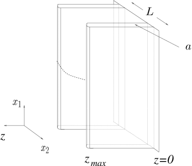
Figure 3: The interaction between two rectangular Wilson loops of size $a$, separated by a distance $L\gg a$.

$$\begin{split}V=&-\lim_{T\rightarrow\infty}\frac{\log\langle W(\CC,L)W(\CC,0)\rangle-\log\langle W(\CC,L)\rangle\langle W(\CC,0)\rangle}{T}\\ =&\sum_{n}V_{n}\frac{a^{2n-2}}{L^{2n-1}}.\end{split}$$ (4.21)

Perturbatively, we will find that the $V_{n}\sim\lambda^{p}/N^{2}$. At large $\lambda$, the $N$ dependence is the same, but the $\lambda$ dependence will be different.

We will use the worldsheet solutions of [4] to compute the effective potential. We find that, for large separations, the asymptotic behavior of the scalar Green’s function (A.9) is

$$G_{k}(x,x^{\prime})={\alpha_{0,k}\over A}\left(\frac{zz^{\prime}}{L^{2}+(\tau-\tau^{\prime})^{2}}\right)^{\Delta}+\cdots.$$ (4.22)

The surface was given by

$$x(z)=z_{max}\int_{z/z_{max}}^{1}dy\frac{{y}^{2}}{\sqrt{1-y^{4}}},$$ (4.23)

where $z_{max}$ is determined by the condition that $|x(0)-x(z_{max})|=a/2$, so that $z_{max}=a\Gamma(1/4)^{2}/(2\pi)^{3/2}$. The area element is given by

$$d{\cal A}=dt\,dz\,\frac{z_{max}^{2}}{z^{2}\sqrt{z_{max}^{4}-z^{4}}}.$$ (4.24)

The coupling to the field $s$ is given by

$$S={1\over 2\pi\alpha^{\prime}}\int d{\cal A}{(-2ks)z^{2}\over z_{max}^{2}},$$ (4.25)

where we used the same method as above to calculate the coupling involving terms with derivatives of $s$. So the final expression for the potential between two Wilson loops is

$$\begin{split}V^{({s})}=&-\frac{S^{({s})}}{T}\\ &=-\sum_{k,A}{\alpha_{0}\over B_{k}}\,{\Gamma(k-1/2)\sqrt{\pi}\over\Gamma(k)L^{2k-1}}\,\left[\frac{(-2k)z_{max}^{k-1}}{2\pi\alpha^{\prime}}\,{\sqrt{\pi}\Gamma(\tfrac{k+1}{4})\over 4\Gamma(\tfrac{k+3}{4})}\right]^{2}Y^{(k)}_{A}(\theta)^{2}\\ &=-\sum_{k}\frac{\Gamma(\tfrac{1}{4})^{4k-4}}{32^{2k+5}\pi^{3k-7/2}}\,\frac{k(k+1)^{2}(k+2)(k+3)\Gamma(k-\tfrac{1}{2})\Gamma(\tfrac{k+1}{4})^{4}}{\Gamma(k)\Gamma(\tfrac{k+1}{2})^{2}}\,\frac{g_{s}N}{N^{2}}\frac{a^{2k-2}}{L^{2k-1}}.\end{split}$$ (4.26)

We have done the sum $\sum_{A}Y^{k}_{A}(\theta)^{2}=(k+3)(k+2)/(3\cdot 2^{k+1})$. We have included contributions to the potential coming from all of the Kaluza-Klein modes of the field $s$. The ones with $k=2$ will give the leading contribution. Of course other fields will also make contributions to the potential which are comparable to the terms above with $k\geq 3$. For example, we can calculate the contributions to the potential from the dilaton

$$\begin{split}V^{\phi}=&-\sum_{k,m_{k}}{\alpha_{0}\over{B^{\prime}_{k}}}\,{\Gamma(\Delta-1/2)\sqrt{\pi}\over\Gamma(\Delta)L^{2\Delta-1}}\,\left[\frac{(1/2)z_{max}^{\Delta-1}}{2\pi\alpha^{\prime}}{\sqrt{\pi}\Gamma(\tfrac{\Delta-1}{4})\over 4\Gamma(\tfrac{\Delta+1}{4})}\right]^{2}Y^{(k)}_{m_{k}}(\theta)^{2}\\ =&-\sum_{k}\frac{\Gamma(\tfrac{1}{4})^{4\Delta-4}}{32^{2\Delta+9}\pi^{3\Delta-7/2}}\,\frac{(\Delta-1)^{2}(\Delta-2)^{2}(\Delta-3)\Gamma(\Delta-\tfrac{1}{2})\Gamma(\tfrac{\Delta-1}{4})^{4}}{\Gamma(\Delta)\Gamma(\tfrac{\Delta-1}{2})^{2}}\\ &\hskip 71.13188pt\cdot\frac{g_{s}N}{N^{2}}\frac{a^{2\Delta-2}}{L^{2\Delta-1}},\end{split}$$ (4.27)

where now $\Delta=4+k$. As $g_{s}\sim\lambda/N$, these results agree with the behavior illustrated in (4.21).

4.4 Contributions from Vectors and Tensors

Let us finally note that the operator product coefficients involving other operators can be computed in a similar way. They will involve the contribution of various supergravity fields to the correlator between two different Wilson loops. In particular, the term $\text{tr}(X^{I}F_{\mu\nu})$ term in the OPE (2.4) corresponds to the lowest mode of an antisymmetric tensor, $B_{\mu\nu}$, on AdS₅.

5 The Spherical Wilson Surface and AdS₇

In [4], it was shown that one could use the AdS description of the large $N$ limit of the $(0,2)$ superconformal field theory in six dimensions to compute Wilson surface observables [13], even though an explicit formulation of the field theory does not exist, so that there is no formula analogous to (2.2). Let us consider a spherical Wilson surface. We take the scalar charge of the surface to be constant (a point on $S^{4}$). In the gravity picture, the Wilson surface should be the boundary of a minimal area membrane worldvolume in AdS${}_{7}\times S^{4}$. One can either solve the equations of motion directly to obtain the minimal worldvolume, or, by analogy with the discussion of section 3, one can note that a flat plane in the boundary of AdS₇ can be conformally mapped to a sphere. This flat plane is the boundary of an infinite membrane that is stretched between the AdS boundary and $z=\infty$. The conformal mapping maps the worldvolume into a 3-hemisphere whose boundary is a 2-sphere that corresponds to the CFT Wilson surface. A convenient parameterization of the solution is given in terms of the Poincare coordinates as

$$\begin{split}x_{1}&=\sqrt{a^{2}-z^{2}}\cos\theta\\ x_{2}&=\sqrt{a^{2}-z^{2}}\sin\theta\cos\psi\\ x_{3}&=\sqrt{a^{2}-z^{2}}\sin\theta\sin\psi,\end{split}$$ (5.1)

where $0\leq z\leq a$, $0\leq\theta\leq\pi$, and $0\leq\psi\leq 2\pi$. Now we take the radius of $AdS$ to be equal to one, then the radius of $R_{S_{4}}=1/2$, $l_{p}=1/(8\pi N)^{1/3}$, and the tension of the two-brane is $T^{(2)}=1/(2\pi)^{2}l_{p}^{3}=2N/\pi$.

We then find that the volume of the membrane is divergent

$$\begin{split}S&=T^{(2)}\int d{\cal V}=T^{(2)}4\pi\int_{\epsilon}^{a}\frac{dz\,a\sqrt{a^{2}-z^{2}}}{z^{3}}\\ &=\pi T^{(2)}\left[+\frac{2a^{2}}{\epsilon^{2}}-2\ln\frac{2a}{\epsilon}-1+{\cal O}(\epsilon)\right].\end{split}$$ (5.2)

We can make several observations regarding this expression for the action. First, we see that the action scales as $N$, in agreement with the scaling found for the “rectangular” solution of [4]. As indicated in [7], $\epsilon$ should be thought of as a UV cutoff. So we see that we have two divergent terms. The quadratic divergence is proportional to the area of the surface. This term was also present in the case of a rectangular Wilson surface [4]. In this case, we see that there is also a logarithmic divergence. The first question is what would this divergence be in a more general case? It can be seen, by analyzing the equations of motion of the theory, that for a generic two-dimensional surface $\Sigma_{2}$ this logarithmic divergence is proportional to the “rigid string” action [14]

$$S_{rigid}=\int_{\Sigma_{2}}d^{2}\sigma\sqrt{\gamma}(\nabla^{2}X^{i})^{2},$$ (5.3)

where $\gamma$ is the induced metric on the Wilson surface and $X^{i}$ are the coordinates on $\BR^{6}$ describing the surface. Notice that $\Sigma_{2}$ is a surface in the boundary six-dimensional field theory. As emphasized in [14], this action is invariant under scale transformations in the target space, $X^{i}\to\lambda X^{i}$, which is consistent with what we expect in a conformal theory. Actually, it is possible to prove that the action is also invariant under special conformal transformations, so that it is invariant under the full conformal group. One implication of this logarithmic term is that the expectation value of the Wilson surface is not well defined, since we can add any constant to the logarithmic subtraction. Furthermore, it seems to indicate that the expectation value of a Wilson surface is scale dependent.

It seems natural to speculate that tensionless strings in this six-dimensional field theory are governed by some supersymmetric form of the the action (5.3).

Despite the fact that the expectation value of the spherical Wilson surface is not well defined, the connected correlation functions of Wilson surfaces do not receive extra divergent contributions. These correlators can be calculated in a completely analogous fashion to the Wilson loops in section 4. One considers a Wilson surface whose characteristic size is much smaller than its distance from any probe in the theory. Then one identifies the operators that are allowed to appear in the OPE and computes the necessary correlation functions to extract the OPE coefficients. The details will appear in [15].

6 Conclusions

In this paper, we have made use of the the connection between Anti–de Sitter spaces and conformal field theories in the large $N$ and $g_{YM}^{2}N$ limit to compute the operator product expansion of “small” Wilson loops in $\CN=4$, $d=4$ super Yang-Mills theory and Wilson surfaces in the $(0,2)$ superconformal theory in six dimensions.

By determining what supergravity states couple to the worldsheet describing the Wilson loop, we found the set of operators that are allowed to appear in the OPE. By computing the amplitudes for exchange of supergravity modes between a Wilson loop and the boundary and between two Wilson loops, we were able to compute the correlation functions of a Wilson loop with a CFT operator and with another loop. From these expressions, we were able to deduce the coefficients that appear in the OPE for the states that we considered.

We also investigated Wilson surfaces in the (0,2) six-dimensional field theory and we found that there is a UV logarithmically divergent contribution to its expectation value proportional to the action of a rigid string embedded in the 5-brane worldvolume.

Appendix A Green’s Functions

Scalar Green’s functions on anti-de Sitter space have been discussed in a large number of papers [3, 2, 16, 17, 18, 19] in connection with the types of correlation functions we are looking to compute. We will repeat some of these calculations in this appendix.

Consider the action of a real scalar field $\phi$ on Euclidean anti- de Sitter spacetime, of radius one, with source $J$,

$$S=\int_{AdS}d^{d+1}x\,\sqrt{g}\,B\left[\frac{1}{2}(d\phi)^{2}+\frac{m^{2}}{2}\phi^{2}-\phi J\right].$$ (A.1)

where $B$ is some constant. The equation of motion is

$$B(-\nabla^{2}_{x}+m^{2})\phi=J,$$ (A.2)

where $\nabla^{2}_{x}=\frac{1}{\sqrt{g}}\partial_{\mu}(\sqrt{g}g^{\mu\nu}\partial_{\nu})$ is the Laplacian. Imposing the boundary condition $\phi|_{\partial M}=0$ yields a unique solution for $\phi$, as long as the operator $-\nabla^{2}_{x}+m^{2}$, is positive definite. This is the case for all $m^{2}\geq-d^{2}/4$ [20].

Solutions for $\phi$ which minimize the action (A.1) are given by the integral equation

$$\phi(x)=\int_{M}d^{d+1}x^{\prime}\sqrt{g(x^{\prime})}\,G(x,x^{\prime})J(x^{\prime}),$$ (A.3)

where the kernel $G(x,x^{\prime})$ is the covariant Green’s function for the equation of motion (A.2), satisfying

$$B(-\nabla^{2}_{x}+m^{2})G(x,x^{\prime})=\frac{1}{\sqrt{g(x^{\prime})}}\delta^{(d+1)}(x-x^{\prime}).$$ (A.4)

By evaluating the action at a solution of (A.3), one finds that

$$S=-\frac{1}{2}\int_{M}d^{d+1}x\,\int_{M^{\prime}}d^{d+1}x^{\prime}\,\sqrt{g(x)}\,J(x)\,G(x,x^{\prime})\,\sqrt{g(x^{\prime})}\,J(x^{\prime}).$$ (A.5)

If we consider the specific case of two separated sources, $J_{1}(x)$ and $J_{2}(x^{\prime})$, the amplitude for their interaction is then given by

$$S=-\int_{M}d^{d+1}x\,\int_{M^{\prime}}d^{d+1}x^{\prime}\,\sqrt{g(x)}\,J_{1}(x)\,G(x,x^{\prime})\,\sqrt{g(x^{\prime})}\,J_{2}(x^{\prime}).$$ (A.6)

A.1 Bulk–to–Bulk Scalar Green’s Functions

We will find it most convenient to compute the Green’s function in the upper-half space representation of anti-de Sitter spacetime, with metric

$$ds^{2}=\frac{1}{z^{2}}\left(dz^{2}+\sum_{i=1}^{d}dx_{i}^{2}\right).$$ (A.7)

As the scalar Green’s function can only depend on the distance $d(x,x^{\prime})$ between the sources, in this metric it will be a function of

$$W=\frac{zz^{\prime}}{(z-z^{\prime})^{2}+\sum_{i=1}^{d}|x_{i}-x_{i}^{\prime}|^{2}}=\frac{1}{2}\,\frac{1}{\cosh d(x,x^{\prime})-1}.$$ (A.8)

Note that $W$ is singular precisely at $(z,x)=(z^{\prime},x^{\prime})$, which is the location of the singularity in the Green’s function (A.4). It is easy to show that the solution for (A.4) which goes to zero at the boundary is given in terms of the hypergeometric function

$$G(W)={\alpha_{0}\over B}W^{\Delta}\,{{}_{2}}F_{1}(\Delta,\Delta+\tfrac{1-d}{2},2\Delta-d+1;-4W).$$ (A.9)

where $\Delta=d/2+\sqrt{m^{2}+d^{2}/4}$ will be the conformal weight of the associated operator and $\alpha_{0}$ is

$$\begin{split}\alpha_{0}=&\frac{\Gamma(\Delta)}{2\pi^{\frac{d}{2}}\Gamma(\Delta-{d\over 2}+1)}\\ \alpha_{0}=&\frac{\Delta-1}{2\pi^{2}}~{}~{}~{}~{}~{}~{}~{}~{}~{}~{}~{}~{}{\rm for}~{}~{}d=4\\ \end{split}$$ (A.10)

A.2 Computation of correlation functions

Let us consider the field in the bulk (A.3) produced by a source on the boundary. To be precise, we take $J(x^{\prime})$ to have support very close to the boundary,

$$\text{supp}\bigl{(}J(x^{\prime})\bigr{)}=\{z^{\prime}|0\leq z^{\prime}<\epsilon\},\$$ (A.11)

for infinitesimal $\epsilon$. Then, using the bulk-to-bulk Green’s function (A.9), we can write

$$\phi(x)=\int_{\partial M}d^{d}x^{\prime}\int_{0}^{\epsilon}dz^{\prime}\,\sqrt{g(x^{\prime})}\,G(x,x^{\prime})J(x^{\prime}).$$ (A.12)

In the region over which we integrate $z^{\prime}$, $W\sim 0$, so that we can approximate

$$G(W)\sim{\alpha_{0}\over B}W^{\Delta},$$ (A.13)

so that

$$\phi(x)\sim{\alpha_{0}\over B}\int_{\partial M}d^{d}x^{\prime}\left(\frac{z}{z^{2}+|\vec{x}-\vec{x}^{\prime}|^{2}}\right)^{\Delta}\int_{0}^{\epsilon}dx_{0}^{\prime}\,{z}^{\Delta-d-1}J(x^{\prime}).$$ (A.14)

Now, to make contact with Witten’s analysis in [3], we want to define a dimension $d-\Delta$ source $\phi_{0}(\vec{x}^{\prime})$.

$$\phi_{0}(\vec{x}^{\prime})=c\int_{0}^{\epsilon}dz^{\prime}\,{z^{\prime}}^{\Delta-d-1}J(x^{\prime}),$$ (A.15)

where $c$ is a numerical factor which we will determine from the 2-point function. Now, evaluating the action obtained from (A.6), we find that

$$\begin{split}S=&{\alpha_{0}\over B}\int d^{d}x\,d^{d}x^{\prime}\,\frac{1}{|\vec{x}-\vec{x}^{\prime}|^{2\Delta}}\int dz\,z^{\Delta-d-1}J(x)\,\int dz^{\prime}\,{z^{\prime}}^{\Delta-d-1}J(x)\\ =&\frac{\alpha_{0}}{Bc^{2}}\int d^{d}x\,d^{d}x^{\prime}\,\frac{\phi_{0}(\vec{x})\phi_{0}(\vec{x}^{\prime})}{|\vec{x}-\vec{x}^{\prime}|^{2\Delta}}.\end{split}$$ (A.16)

The two-point function is then

$$\frac{\delta^{2}S}{\delta\phi_{0}(\vec{x})\delta\phi_{0}(\vec{x}^{\prime})}=\frac{\alpha_{0}}{Bc^{2}}\,\frac{1}{|\vec{x}-\vec{x}^{\prime}|^{2\Delta}}.$$ (A.17)

Choosing the convention that the operator corresponding to this scalar is unit-normalized, $\langle\CO\CO\rangle=1/x^{2\Delta}$, we determine that $c=\sqrt{\alpha_{0}/B}$.

References

- [1] J. Maldacena, “The large limit of superconformal field theories and supergravity,” Adv. Theor. Math. Phys. 2 (1998) hep-th/9711200.
- [2] S. S. Gubser, I. R. Klebanov, and A. M. Polyakov, “Gauge theory correlators from noncritical string theory,” Phys. Lett. B428 (1998) 105, hep-th/9802109.
- [3] E. Witten, “Anti-de Sitter space and holography,” Adv. Theor. Math. Phys. 2 (1998) hep-th/9802150.
- [4] J. Maldacena, “Wilson loops in large field theories,” Phys. Rev. Lett. 80 (1998) 4859–4862, hep-th/9803002.
- [5] S.-J. Rey and J. Yee, “Macroscopic strings as heavy quarks in large gauge theory and anti-de Sitter supergravity,” hep-th/9803001.
- [6] D. J. Gross and H. Ooguri, “Aspects of large gauge theory dynamics as seen by string theory,” hep-th/9805129.
- [7] L. Susskind and E. Witten, “The holographic bound in anti-de Sitter space,” hep-th/9805114.
- [8] S. Lee, S. Minwalla, M. Rangamani, and N. Seiberg, “Three-point functions of chiral operators in , SYM at large ,” hep-th/9806074.
- [9] D. J. Gross, “Aspects of large gauge theory dynamics as seen by string theory,” in Strings ’98 (Santa Barbara, CA, June 22-27, 1998), S. Giddings, H. Ooguri, A. Peet, and J. Schwarz, eds. Online proceedings at http://www.itp.ucsb.edu/~strings98.
- [10] H. J. Kim, L. J. Romans, and P. van Nieuwenhuizen, “Mass spectrum of chiral ten-dimensional supergravity on ,” Phys. Rev. D32 (1985) 389.
- [11] V. Balasubramanian, P. Kraus, A. Lawrence, and S. P. Trivedi, “Holographic probes of anti-de Sitter space-times,” hep-th/9808017.
- [12] M. E. Peskin, “Short distance analysis for heavy-quark systems. (I). Diagrammatics,” Nucl. Phys. B156 (1979) 365.
- [13] O. J. Ganor, “Six-dimensional tensionless strings in the large limit,” Nucl. Phys. B489 (1997) 95–121, hep-th/9605201.
- [14] A. M. Polyakov, “Fine structure of strings,” Nucl. Phys. B268 (1986) 406.
- [15] R. Corrado, B. Florea, and R. McNees. To appear.
- [16] R. G. Leigh and M. Rozali, “The large limit of the superconformal field theory,” Phys. Lett. B431 (1998) 311–316, hep-th/9803068.
- [17] W. Mück and K. S. Viswanathan, “Conformal field theory correlators from classical scalar field theory on ,” Phys. Rev. D58 (1998) 041901, hep-th/9804035.
- [18] D. Z. Freedman, S. D. Mathur, A. Matusis, and L. Rastelli, “Correlation functions in the CFT correspondence,” hep-th/9804058.
- [19] G. Chalmers, H. Nastase, K. Schalm, and R. Siebelink, “R current correlators in super Yang-Mills theory from anti-de Sitter supergravity,” hep-th/9805105.
- [20] P. Breitenlohner and D. Z. Freedman, “Positive energy in anti-de Sitter backgrounds and gauged extended supergravity,” Phys. Lett. B115 (1982) 197.