PERTURBATIVE RELATIONSHIPS BETWEEN QCD AND GRAVITY AND SOME IMPLICATIONS

Abstract

We discuss nontrivial examples illustrating that perturbative gravity is in some sense the ‘square’ of gauge theory. This statement can be made precise at tree-level using the Kawai, Lewellen and Tye relations between open and closed string tree amplitudes. These relations, when combined with modern methods for computing amplitudes, allow us to obtain loop-level relations, and thereby new supergravity loop amplitudes. The amplitudes show that $N=8$ supergravity is less ultraviolet divergent than previously thought. As a different application, we show that the collinear splitting amplitudes of gravity are essentially squares of the corresponding ones in QCD.

1 Introduction

Although QCD and general relativity are similar theories in that they both possess local symmetries and mediate forces, their Lagrangians are rather different. In particular, gravity contains an infinite number of interaction vertices, whereas QCD contains only three- and four-point vertices. In this talk we discuss examples demonstrating that the perturbative $S$-matrices of gravity and QCD are more closely related than expected based on their Lagrangians.

The existence of relations between gravity and gauge theory amplitudes may be understood from string theory. At tree level, Kawai, Lewellen and Tye [1] (KLT) have given precise relations between closed and open string theory amplitudes. These relations follow (after deforming integration contours) from the factorization of a closed string integrand into the product of two open string integrands, one for left-movers and one for right-movers. In the infinite string tension limit, where string theory reduces to field theory, the KLT relations indicate that

$$\hbox{gravity}\sim\hbox{(gauge theory)}\times\hbox{(gauge theory)}\,.$$

In this talk we explain how this relationship can be made precise at loop level. More importantly, we shall discuss its use in acquiring nontrivial information about (super) gravity. The key to exploiting relation ($(1)$) is to apply modern methods for computing amplitudes, including improved cutting methods, helicity and color decompositions. (For a discussion of these methods and for references, see previous reviews [2, 3].)

As a simple illustration of the notion contained in eq. ($(1)$), we show that splitting amplitudes, which describe the behavior of the gravity $S$-matrix as the momenta of two external legs become collinear, are given by products of gauge theory splitting amplitudes.

Another application that we discuss is an investigation of the divergences in $N=8$ supergravity, based on recycling similar gauge theory calculations [4]. Our interest in $N=8$ supergravity stems from the fact that it is expected to be the least divergent of all field theories of gravity. Furthermore, its high degree of symmetry considerably simplifies the analytic structure of amplitudes, allowing for relatively simple computations. As an important side benefit, it allows us to test methods for computing multi-loop amplitudes in more phenomenological theories such as QCD.

The study of divergences in gravity theories has a long history [5, 6]. Because Newton’s coupling $G_{N}=\kappa^{2}/32\pi$ is dimensionful, the presence of an ultraviolet divergence indicates that a theory of gravity is not fundamental, and that another type of theory, such as string or $M$ theory, may be required. Except for the explicit calculation of the two-loop divergence in pure gravity by Goroff and Sagnotti, and later by van de Ven, analyses of the divergences have generally been based on determining the form of potential counterterms, subject to power-counting of loop momenta and symmetry considerations. However, it is always possible that the coefficient of a potential counterterm can vanish, especially if the full symmetry of the theory is not taken into account.

One-loop amplitudes and divergences in $N=8$ supergravity were first calculated via string theory [7]. We have computed the two-loop $N=8$ supergravity amplitude in field theory, by relating its unitarity cuts to double copies of the cuts of the corresponding $N=4$ super-Yang-Mills amplitude. In fact, the two-particle cut calculation can be iterated to generate part of the amplitude at an arbitrary loop order. Based on this evidence, we shall argue that $N=8$ supergravity is less divergent than previously thought. In particular, the cut calculations indicate that in $D=4$ the first divergence in four-point amplitudes occurs at five loops, contrary to previous expectations of three loops [6]. Since superspace power-counting only places bounds on allowed divergences, there is no real contradiction. While it may seem of little importance whether the divergence starts at five as opposed to three loops, so long as there is a divergence, the point we wish to stress is that the relation ($(1)$) between gauge theories and gravity theories can be sharpened and exploited to investigate properties of gravity theories.

2 Gravity and Yang-Mills at Tree-Level

2.1 Lagrangians

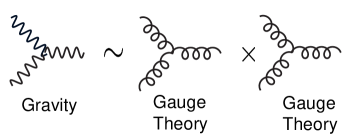
Figure 1: String theory suggests that the three-graviton vertex can be expressed as a product of three-gluon vertices.

Before discussing the $S$-matrices, we comment on the Lagrangians of gravity, ${\cal L}_{\rm gravity}=\sqrt{g}R$, and Yang-Mills, ${\cal L}_{\rm YM}=-{1\over 4}F^{a}_{\mu\nu}F^{a\,\mu\nu}$. Although the Lagrangians appear to be rather different, eq. ($(1)$) suggests that the interaction vertices should be related. In particular, one might expect that the gravity three-vertex can be factorized as a product of gauge theory three-vertices, as depicted in fig. 1. However, such relations do not hold in the standard de Donder (harmonic) gauge for gravity, in which the three-vertex is [8],

$$G^{\rm harmonic}_{3\mu\alpha,\nu\beta,\rho\gamma}(k_{1},k_{2},k_{3})\ \sim\ k_{1}\cdot k_{2}\eta_{\mu\alpha}\eta_{\nu\beta}\eta_{\rho\gamma}\ +\ \hbox{many other terms}\,.$$

The exhibited term contains traces over the index pairs of gravitons, which prevent the three-graviton vertex from factorizing.

In order for the relation depicted in fig. 1 to hold, one has to carefully choose gauges and field variables. In particular, in the background-field [9] versions of de Donder gauge for gravity and of Feynman gauge for QCD, one finds (after color ordering and stripping the gluon vertex of color factors) that the relation in fig. 1 does indeed hold [10]. However, this solution is not completely satisfactory; it becomes increasingly obscure to go beyond three points. Furthermore, background field gauges are meant for loop effective actions and not for the (tree-level) $S$-matrix elements.

In multi-loop gravity Feynman diagram calculations, the number of algebraic terms proliferates rapidly beyond the point where computations are practical. Consider the five-loop diagram in fig. 2 (which is of interest for ultraviolet divergences in $N=8$ supergravity in $D=4$). In de Donder gauge this diagram contains twelve vertices, each of the order of a hundred terms, and sixteen graviton propagators, each with three terms, for a total of roughly $10^{30}$ terms. Needless to say, this is well beyond what can be reasonably implemented on any computer. Furthermore, standard methods for simplifying diagrams, such as background-field gauges and superspace, are unfortunately insufficient for dealing with problems of this complexity. Direct string theory based calculations are also not as yet practical for performing multi-loop calculations, since they are beset with a variety of technical difficulties.

Our approach will instead be to use cutting methods developed for QCD computations [11, 12, 3] to exploit the relation ($(1)$) and allow us to bypass Feynman diagram computations.

Figure 2: An example of a five loop diagram.

2.2 Kawai-Lewellen-Tye Tree-Level String Relations

At tree level, KLT [1] showed that closed string amplitudes could be expressed as bilinear sums of open string amplitudes. The same relations hold for any set of closed string states, using their Fock space factorization into pairs of open string states. In the infinite string tension limit, where string theory reduces to field theory, $N=8$ supergravity amplitudes are related to $N=4$ Yang-Mills amplitudes [13], making relation ($(1)$) precise at tree level. The four- and five-point KLT relations are,

 

$${M_{4}^{\rm tree}(1,2,3,4)}$$

 

where $s_{ij}=(k_{i}+k_{j})^{2}$, the $A_{n}$ are color-ordered gauge theory amplitudes, and the $M_{n}$ are gravity amplitudes. The arguments of the amplitudes label the external legs. For simplicity we have also suppressed coupling constants and our normalization conventions [4].

The tree amplitudes with only external gluons are exactly the same ones that appear in QCD, because the other fields in the $N=4$ multiplet cannot appear in intermediate states. Similarly, the gravity amplitudes are those of ordinary Einstein gravity.

Berends, Giele and Kuijf [13] exploited the KLT relations ($(3)$) and their $n$-point generalizations to obtain an infinite set of maximally helicity violating (MHV) gravity tree amplitudes, using the known MHV Yang-Mills amplitudes [14]. Here we shall explain how one can use the KLT relations to compute multi-loop gravity amplitudes, starting from gauge theory amplitudes. First, though, we discuss a simpler application of the KLT relations: the derivation of collinear splitting amplitudes in gravity from those in QCD.

3 Behavior of Gravity Amplitudes for Collinear Momenta.

QCD helicity amplitudes have a well-known behavior as momenta of external legs become collinear or soft [2, 3]. In the case of gravity, only the soft limits have been discussed in detail [15, 13].

At tree-level in QCD, the color-ordered and -stripped amplitudes have the following behavior as the momenta of legs $1$ and $2$ become collinear ($k_{1}\rightarrow zP$, $k_{2}\rightarrow(1-z)P$, and $P=k_{1}+k_{2}$):

$$A_{n}^{\rm tree}(1,2,\ldots,n)\ \mathop{\longrightarrow}^{k_{1}\parallel k_{2}}\ \sum_{\lambda=\pm}\mathop{\rm Split}\nolimits_{-\lambda}^{\rm QCD\ tree}(1,2)\,A_{n-1}^{\rm tree}(P^{\lambda},3,\ldots,n)\,,$$

where $\mathop{\rm Split}\nolimits_{-\lambda}^{\rm QCD\ tree}(1,2)$ is a splitting amplitude, and $\lambda$ is the helicity of the intermediate state $P$. (The other helicity labels have been suppressed.) For the pure glue case, one such splitting amplitude is

$$\mathop{\rm Split}\nolimits_{-}^{\rm QCD\ tree}(1^{+},2^{+})={1\over\sqrt{z(1-z)}}\,{1\over\left\langle 1\,2\right\rangle}\,,$$

where the ‘$+$’ and ‘$-$’ labels refer to the helicity of the gluons,

 

$${\left\langle j\,l\right\rangle}$$

 

are spinor inner products, and $\phi_{jl}$ is a momentum-dependent phase [2].

From Feynman diagrams (or from the structure of the $n$-point KLT relations) one can argue that the universal relation ($(4)$) must hold for gravity too [16], with $A$ replaced by $M$, and $\mathop{\rm Split}\nolimits^{\rm QCD\ tree}$ replaced by a suitable gravitational splitting amplitude, $\mathop{\rm Split}\nolimits^{\rm gravity\ tree}$. The KLT relations ($(3)$) give a simple way to determine $\mathop{\rm Split}\nolimits^{\rm gravity\ tree}$. Universality permits us to consider any particular collinear limit. Taking $k_{1}\parallel k_{2}$ in the five-point relation ($(3)$), we find

$$\mathop{\rm Split}\nolimits^{\rm gravity\ tree}(1,2)=-s_{12}\times\mathop{\rm Split}\nolimits^{\rm QCD\ tree}(1,2)\times\mathop{\rm Split}\nolimits^{\rm QCD\ tree}(2,1)\,.$$

More explicitly, using eq. ($(5)$) for example, we find that

$$\mathop{\rm Split}\nolimits_{-}^{\rm gravity\ tree}(1^{+},2^{+})={-1\over z(1-z)}{\left[1\,2\right]\over\left\langle 1\,2\right\rangle}\,.$$

The $s_{12}$ factor has canceled the pole, although a phase singularity remains, from the form of the spinor inner products given in eq. ($(6)$); the phase factor $\phi_{12}$ rotates by $2\pi$ as $\vec{k}_{1}$ and $\vec{k}_{2}$ rotate once around their sum $\vec{P}$. The corresponding $4\pi$ rotation in eq. ($(8)$) accounts for the angular-momentum mismatch of 2$\hbar$ between the graviton $P^{+}$ and the pair of gravitons $(1^{+},2^{+})$.

In the gauge theory case, the splitting amplitude terms ($(4)$) dominate the collinear limit; sub-leading behavior is down by a power of $\sqrt{s_{12}}$. In the gravitational analog of eq. ($(4)$), the meaning is different: There are other terms of the same magnitude as $\left[1\,2\right]/\left\langle 1\,2\right\rangle$ as $s_{12}\to 0$; however, these non-universal terms do not acquire any additional phase as $\vec{k}_{1}$ and $\vec{k}_{2}$ are rotated, and thus they can be meaningfully separated from the universal terms.

One application of collinear limits is to help determine the analytic structure of the graviton $S$-matrix. In gauge theory, such information has been used to find precise expressions for $S$-matrix elements [17, 11, 18]. Using the soft and collinear properties of gravity we have succeeded in constructing Ansätze for MHV one-loop amplitudes with an arbitrary number of external legs. These results will be discussed elsewhere [16], along with a more complete presentation of the collinear and soft properties of gravity amplitudes.

4 Multi-Loop Calculations

Over the years there have been a number of rather impressive multi-loop Feynman diagram calculations. However, a number of important computations remain to be performed. Two examples of QCD computations that are required for analyses of experiments, but have not yet been carried out, are the two-loop contributions to $e^{+}\,e^{-}\rightarrow 3$ jets and to the Altarelli-Parisi splitting functions. The $e^{+}\,e^{-}\rightarrow 3$ jets calculation would be important, for example, for reducing theoretical errors in the extraction of $\alpha_{s}$ from the jet data. More generally, no computations have appeared at two and higher loops that involve more than a single kinematic variable.

At one loop, a successful recent approach has been to reconstruct amplitudes from their kinematic poles and cuts [3]. This approach was used to obtain infinite sequences of one-loop MHV amplitudes in QCD [17] and in supersymmetric versions of QCD [11], as well as the one-loop helicity amplitudes for $e^{+}\,e^{-}\rightarrow 4$ partons [18]. Here we will apply the same techniques to two-loop four-point amplitudes in $N=4$ super-Yang-Mills theory and $N=8$ supergravity.

4.1 Cutting Methods

The cutting method for computing helicity amplitudes has been extensively discussed for the case of gauge theory amplitudes [11, 3], so here we only briefly describe it. The unitarity cuts of a loop amplitude are given by phase-space integrals of products of amplitudes containing fewer loops. For example, the cut for a one-loop four-point amplitude in the channel carrying momentum $k_{1}+k_{2}$, as shown in fig. 3, is given by

 

$${\sum_{\rm states}\int}$$

 

where $\ell_{2}=\ell_{1}-k_{1}-k_{2}$, and the sum runs over all states crossing the cut. (Polarization labels have been suppressed.) We apply the on-shell conditions $\ell_{1}^{2}=\ell_{2}^{2}=0$ even though the loop momentum is unrestricted; only functions with a cut in the given channel are reliably computed in this way. (The positive energy conditions are automatically imposed by the use of Feynman propagators.)

Figure 3: The two-particle cut at one loop in the channel carrying momentum $k_{1}+k_{2}$.

Complete amplitudes are found by combining all cuts into a single function with the correct cuts in all channels. If one works with an arbitrary dimension $D$ in eq. ($(9)$), and takes care to keep the full analytic behavior as a function of $D$, then the results will be free of the usual subtraction ambiguities of cutting methods [12, 3]. (The regularization scheme dependence remains, of course.)

An important advantage of the cutting approach is that the gauge-invariant amplitudes on either side of the cut can be simplified before attempting to evaluate the cut integral [3]. In the case of gravity, we can also make use of the KLT relations to find convenient representations of the tree amplitudes for gravity [4] in terms of the ones for gauge theory.

4.2 Maximally Supersymmetric Theories

The higher degree of symmetry in supersymmetric amplitudes suggests that they should have a simpler analytic structure than non-supersymmetric theories such as QCD or Einstein gravity. Therefore, it is logical to investigate them first. In particular, amplitudes in the maximally supersymmetric theories, $N=4$ super-Yang-Mills and $N=8$ supergravity, should be especially simple; indeed, this is the case at one loop [7, 11, 19]. We first discuss multi-loop $N=4$ super-Yang-Mills amplitudes, then recycle the answers (using the KLT relations) to get corresponding results for $N=8$ supergravity, from which we can extract ultraviolet divergences.

4.3 $N=4$ Super-Yang-Mills Multi-Loop Amplitudes.

The key sewing relation used to evaluate the two-particle cuts for $N=4$ four-point amplitudes is [11, 20, 4],

 

$${\sum_{N=4\ \rm states}A_{4}^{\rm tree}(-\ell_{1},}$$

 

where all momenta are on shell and the sum is over all states in the $N=4$ super-multiplet: a gluon, four Weyl fermions and six real scalars. The Mandelstam variables are $s=(k_{1}+k_{2})^{2}$, $t=(k_{1}+k_{4})^{2}$ and $u=(k_{1}+k_{3})^{2}$. Eq. ($(10)$) may be easily checked in a helicity basis using four-dimensional momenta, but it is actually true in all dimensions $(D\leq 10)$ and for all external states belonging to the $N=4$ super-multiplet.

Applying eq. ($(10)$) to eq. ($(9)$) at one-loop and combining the various cuts immediately yields

$$A_{4}^{{1\mbox{-}\rm loop}}(1,2,3,4)=i\,stA_{4}^{\rm{\rm tree}}(1,2,3,4)\,{\cal I}_{4}^{1\mbox{-}\rm loop}(s,t)\,,$$

where

$${\cal I}_{4}^{1\mbox{-}\rm loop}(s,t)=\int{d^{D}\ell\over(2\pi)^{D}}\,{1\over\ell^{2}(\ell-k_{1})^{2}(\ell-k_{1}-k_{2})^{2}(\ell+k_{4})^{2}}\,,$$

in agreement with the previous results of Green, Schwarz and Brink [7].

An important feature of the cutting equation ($(10)$) is that the external-state dependence of the right-hand side is entirely contained in the tree amplitude $A_{4}^{\rm{\rm tree}}$. This fact allows us to iterate the two-particle cut algebra to all loop orders!

Consider now the two-loop case [20]. The two-loop two-particle cut sewing algebra is identical to the one-loop case except for the extra propagators. The three-particle cuts are more involved, but generate no other functions beyond those found with two-particle cuts. After combining all cuts into a single function, a remarkably simple result emerges for the contribution at leading order in the number of colors,

$$A_{4}^{{\rm LC}\ {2\mbox{-}\rm loop}}(1,2,3,4)=-st\,A_{4}^{\rm tree}(1,2,3,4)\,\left(s\,{\cal I}_{4}^{{2\mbox{-}\rm loop},{\rm P}}(s,t)+t\,{\cal I}_{4}^{{2\mbox{-}\rm loop},{\rm P}}(t,s)\right)\,.$$

The non-planar contributions are also simple [20, 4]. The planar and non-planar scalar two-loop integrals that appear in the amplitudes are shown in fig. 4. Closed-form expressions for the scalar integrals in terms of known analytic functions are not yet available; nevertheless, properties such as ultraviolet divergences can be extracted from eq. ($(13)$).

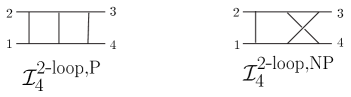
Figure 4: The planar and non-planar scalar integrals, ${\cal I}_{4}^{{2\mbox{-}\rm loop},{\rm P}}(s,t)$ and ${\cal I}_{4}^{{2\mbox{-}\rm loop},{\rm NP}}(s,t)$, appearing in the two-loop $N=4$ and $N=8$ amplitudes. Each internal line represents a scalar propagator.

We have compared [4] the ultraviolet divergences in the above amplitude in $D=7$ and $D=9$ with previous results of Marcus and Sagnotti [21]. Up to a minor, unresolved discrepancy in the overall normalization of the $D=7$ counterterm, we find agreement for both the $D=7$ and $D=9$ counterterms. The agreement is rather nontrivial and provides a strong check on our expressions for the full amplitude.

One may continue to iterate the two-particle cuts to all loop orders. We call an integral function that is successively two-particle reducible into a set of four-point trees ‘entirely two-particle constructible’. Such contributions can be both planar and non-planar. For the planar case, i.e. the large $N_{c}$ ’t Hooft limit, a simple pattern has been noted [20] that generates the entirely two-particle constructible contributions. By extending this to contributions that require three- or higher particle cuts, one obtains an ansatz for the form of all large $N_{c}$ contributions. (Further details may be found in refs. [20, 4].) The ansatz has the expected leading-log BFKL [22] behavior in the $s\rightarrow\infty$ limit. In this limit the gluons dominate, so the result for $N=4$ super-Yang-Mills agrees with that of QCD. This checks that we have the correct ladder diagrams, including normalizations.

4.4 $N=8$ Supergravity Amplitudes

Using the KLT four-point relations in eq. ($(3)$), we may recycle the $N=4$ Yang-Mills sewing equation ($(10)$) into an $N=8$ supergravity sewing equation,

 

$${{}\sum_{N=8\rm\ states}\hskip-8.5359ptM_{4}^{\rm tree}(-\ell_{1},1,2,\ell_{2})\times M_{4}^{\rm tree}(-\ell_{2},3,4,\ell_{1})}$$

 

where the sum runs over all states in the $N=8$ super-multiplet. Given the $N=4$ Yang-Mills two-particle sewing equation ($(10)$), it is a simple matter to evaluate eq. ($(14)$), yielding

 

$${{}\sum_{N=8\rm\ states}M_{4}^{\rm tree}(-\ell_{1},1,2,\ell_{2})\times M_{4}^{\rm tree}(-\ell_{2},3,4,\ell_{1})}$$

 

where we used

$$-i\left(st\,A_{4}^{\rm tree}(1,2,3,4)\right)^{2}=stuM_{4}^{\rm tree}(1,2,3,4)\,,$$

to re-express the prefactor in terms of the $N=8$ tree amplitude. The sewing equations for the $t$ and $u$ channels are similar to that of the $s$ channel.

Applying eq. ($(15)$) at one loop to each of the three channels yields the one-loop amplitude,

 

$${{\cal M}_{4}^{N=8,{{1\mbox{-}\rm loop}}}(1,2,3,4)}$$

 

in agreement with previous results [7]. We have reinserted the gravitational coupling $\kappa$ in this expression. The scalar integrals are the same ones ($(12)$) appearing in the $N=4$ Yang-Mills case.

Because the external-state dependence of the right-hand side of eq. ($(15)$) is contained in the tree amplitude, as in the gauge theory case, the two-loop two-particle cuts are given by a simple iteration of the one-loop calculation. Once again, the three-particle cuts introduce no other functions into the amplitude. Combining the cuts yields the $N=8$ supergravity two-loop amplitude [4],

 

$${{\cal M}_{4}^{{2\mbox{-}\rm loop}}(1,2,3,4)}$$

 

where ‘$+$ cyclic’ instructs one to add the two cyclic permutations of legs (2,3,4), and ${\cal I}_{4}^{{2\mbox{-}\rm loop},{\rm P}/{\rm NP}}$ are depicted in fig. 4. These integrals diverge only for $D\geq 7$; hence the two-loop $N=8$ amplitude is manifestly finite in $D=5$ and $6$, contrary to expectations based on superspace power-counting arguments [6].

Since the two-particle cut sewing equation iterates to all loop orders, one can compute all entirely two-particle constructible contributions, as in the $N=4$ case. (The five-loop integral in fig. 2 falls into this category.) Counting powers of loop momenta in these contributions suggests the simple finiteness formula, $L<10/(D-2)$, where $L$ is the number of loops. This formula indicates that $N=8$ supergravity is finite in some other cases where the superspace bounds suggest divergences [6], e.g. $D=4$, $L=3$. The first $D=4$ counterterm detected via the two-particle cuts of four-point amplitudes occurs at five loops, not three loops. Further evidence that the finiteness formula is correct stems from the MHV contributions to $m$-particle cuts, in which the same supersymmetry cancellations occur as for the two-particle cuts [4]. However, further work is required to prove that other contributions do not alter the two-particle-cut power counting.

Another open question is whether we can prove that the five-loop divergence encountered in the two-particle cuts does not cancel against other contributions. If one could prove that the numerators of all $N=8$ loop-momentum integrals are squares of the corresponding ones for $N=4$ Yang-Mills integrals (i.e. they always appear with the same sign), there would be no need for a detailed investigation of the cuts. The iterated two-particle cuts have the required squaring property, but, as yet, we do not have a more general proof.

5 Conclusions

Gravity and gauge theories are the two cornerstones of modern theoretical physics. In this talk we have discussed nontrivial examples illustrating that perturbative expansions in gravity theories are surprisingly similar to those for gauge theories such as QCD, even though the Lagrangians are rather different. As one example, tree-level collinear splitting amplitudes in gravity were shown to be products of the ones appearing in QCD. For the case of maximally supersymmetric theories, where calculations are relatively simple, we discussed how calculations in $N=4$ super-Yang-Mills can be recycled to get results for $N=8$ supergravity. In particular, we obtained the two-loop four-point amplitudes for each theory in terms of scalar integrals. Furthermore, the two-particle cut calculus iterates to all loop orders. From these considerations, it appears that $N=8$ supergravity is less divergent than previously thought.

It would be nice to find a field theoretic reformulation of gravity where the connection ($(1)$) to gauge theory is explicit. On the more practical side, we are optimistic that the same cutting techniques discussed here can be applied to multi-loop amplitudes in theories with less supersymmetry, such as the two-loop corrections to $e^{+}e^{-}\rightarrow$ 3 jets in QCD.

This research was supported by the US Department of Energy under grants DE-FG03-91ER40662, DE-AC03-76SF00515 and DE-FG02-97ER41029.

References

References

- [1] H. Kawai, D.C. Lewellen and S.-H.H. Tye, Nucl. Phys. B 269, 1 (1986).
- [2] M. Mangano and S.J. Parke, Phys. Rep. 200, 301 (1991); L. Dixon, in Proceedings of Theoretical Advanced Study Institute in Elementary Particle Physics (TASI 95), ed. D.E. Soper [hep-ph/9601359].
- [3] Z. Bern, L. Dixon and D.A. Kosower, Ann. Rev. Nucl. Part. Sci. 46, 109 (1996).
- [4] Z. Bern, L. Dixon, D.C. Dunbar, M. Perelstein and J.S. Rozowsky, Nucl. Phys. B 530, 401 (1998) [hep-th/9802162].
- [5] R.E. Kallosh, Nucl. Phys. B 78, 293 (1974); P. van Nieuwenhuizen and C.C. Wu, J. Math. Phys. 18, 182 (1977); M.H. Goroff and A. Sagnotti, Nucl. Phys. B 266, 709 (1986); A.E.M. van de Ven, Nucl. Phys. B 378, 309 (1992).
- [6] S. Deser, J.H. Kay and K.S. Stelle, Phys. Rev. Lett. 38, 527 (1977); R.E. Kallosh, Phys. Lett. B 99, 122 (1981); P.S. Howe, K.S. Stelle amd P.K. Townsend, Nucl. Phys. B 191, 445 (1981); P.S. Howe and K.S. Stelle, Phys. Lett. B 137, 175 (1984); Int. J. Mod. Phys. A 4, 1871 (1989).
- [7] M.B. Green, J.H. Schwarz and L. Brink, Nucl. Phys. B 198, 474 (1982).
- [8] B.S. DeWitt, Phys. Rev., 162, 1239 (1967); M. Veltman, in Les Houches 1975, Proceedings, Methods In Field Theory (Amsterdam 1976).
- [9] G. ’t Hooft, Acta Universitatis Wratislavensis no. 38, 12th Winter School of Theoretical Physics in Karpacz; Functional and Probabilistic Methods in Quantum Field Theory, Vol. 1 (1975); B.S. DeWitt, in Quantum Gravity II, eds. C. Isham, R. Penrose and D. Sciama (Oxford, 1981); L.F. Abbott, Nucl. Phys. B 185, 189 (1981).
- [10] Z. Bern, D.C. Dunbar and T. Shimada, Phys. Lett. B 312, 277 (1993).
- [11] Z. Bern, L. Dixon, D.C. Dunbar and D.A. Kosower, Nucl. Phys. B 425, 217 (1994); Z. Bern, L. Dixon, D.C. Dunbar and D.A. Kosower, Nucl. Phys. B 435, 59 (1995).
- [12] W.L. van Neerven, Nucl. Phys. B 268, 453 (1986); Z. Bern and A.G. Morgan, Nucl. Phys. B 467, 479 (1996); J.S. Rozowsky, preprint hep-ph/9709423.
- [13] F.A. Berends, W.T. Giele and H. Kuijf, Phys. Lett. B 211, 91 (1988).
- [14] S.J. Parke and T.R. Taylor, Phys. Rev. Lett. 56, 2459 (1986).
- [15] S. Weinberg, Phys. Lett. 9, 357 (1964); Phys. Rev. 140, B516 (1965).
- [16] Z. Bern, L. Dixon, M. Perelstein and J.S. Rozowsky, preprint hep-th/9809160; in preparation.
- [17] Z. Bern, L. Dixon and D.A. Kosower, Proceedings of Strings 1993, eds. M.B. Halpern, A. Sevrin and G. Rivlis (World Scientific, Singapore, 1994); Z. Bern, G. Chalmers, L. Dixon and D.A. Kosower, Phys. Rev. Lett. 72, 2134 (1994); G.D. Mahlon, Phys. Rev. D 49, 2197 (1994); Phys. Rev. D 49, 4438 (1994).
- [18] Z. Bern, L. Dixon, D.A. Kosower and S. Weinzierl, Nucl. Phys. B 489, 3 (1997); Z. Bern, L. Dixon and D.A. Kosower, Nucl. Phys. B 513, 3 (1998).
- [19] D.C. Dunbar and P.S. Norridge, Nucl. Phys. B 433, 181 (1995); D.C. Dunbar and P.S. Norridge, Class. Quant. Grav. 14, 351 (1997).
- [20] Z. Bern, J.S. Rozowsky and B. Yan, Phys. Lett. B 401, 273 (1997); preprint hep-ph/9706392.
- [21] N. Marcus and A. Sagnotti, Nucl. Phys. B 256, 77 (1985).
- [22] E.A. Kuraev, L.N. Lipatov and V.S. Fadin, Phys. Lett. B 60, 50 (1975); Sov. Phys. JETP 44, 443 (1976); Sov. Phys. 45, 199 (1977); Ya. Balitsky and L.N. Lipatov, Sov. J. Nucl. Phys. 28, 822 (1978).