Adrian Patrascioiu

Physics Department, University of Arizona,

Tucson, AZ 85721, U.S.A.

e-mail: patrasci@ccit.arizona.edu

and

Erhard Seiler

Max-Planck-Institut für Physik

(Werner-Heisenberg-Institut)

Föhringer Ring 6, 80805 Munich, Germany

e-mail:ehs@mppmu.mpg.de

Abstract

We report the results of a very high statistics Monte Carlo study of the continuum limit of the two dimensional $O(3)$ non-linear $\sigma$ model. We find a significant discrepancy between the continuum extrapolation of our data and the form factor prediction of Balog and Niedermaier, inspired by the Zamolodchikovs’ $S$-matrix ansatz. On the other hand our results for the $O(3)$ and the dodecahedron model are consistent with our earlier finding that the two models possess the same continuum limit.

In a recent paper [1] we reported some striking numerical results: the continuum limit of the two dimensional ($2D$) $O(3)$ nonlinear $\sigma$ model seems to agree as well with the form factor prediction [2] inpired by Zamolodchikovs’ $S$-matrix as with the continuum limit of the dodecahedron spin model. The latter, known rigorously to possess a phase transition at nonzero temperature, is almost certainly not asymptotically free. Zamolodchikovs’ ansatz on the other hand is believed to embody asymptotic freedom, a belief which was reenforced by some remarkable scaling properties discovered by Balog and Niedermaier [4].

Initially [5] we thought that the resolution of this apparent paradox must come from the absence of asymptotic freedom in the form factor approach and that the scaling proposed by Balog and Niedermaier must actually be false. Soon after though we realized that the trouble was much more serious: indeed from the direct computation of Balog and Niedermaier of the 2,4 and 6 particle contribution it followed that the asymptotic value of the transverse current two point function $J(p)$ must obey the inequality

$$J(\infty)>3.651$$ (1)

[3]. On the other hand in two recent papers [7, 8] we used reflection positivity to prove rigorously an upper bound on $J(\infty)$ in terms of $\beta_{crt}$. In those papers the bound is given only for the $O(2)$ model, but it is straightforward to generalize it to any $O(N)$. For $O(3)$ it reads

$$J(\infty)\leq{2\over 3}\beta_{crt}$$ (2)

Combining these two inequalities one would conclude that $\beta_{crt}>5.5$. This lower bound is so large that irrespective of the Balog and Niedermaier scaling ansatz, it suggests that the critical point may very well be at infinity and the model asymptotically free.

Since, as stated above, asymptotic freedom of $O(3)$ is hard to reconcile with its having the same continuum limit as the dodecahedron spin model, we decided that we needed a more refined numerical study to decide these issues. In the present paper we will report the results of our investigation regarding the continuum limit of the $O(3)$ and dodecahedron spin models. We strove to achieve very high numerical accuracy and to our knowledge our accuracy, exceeding sometimes .05%, has never been achieved before. Our results suggest that in fact the model defined by the form factor approach does not agree with the continuum limit of the $O(3)$ model. On the other hand, the numerical evidence is consistent with the hypothesis that the $O(3)$ and the dodecahedron spin models have the same continuum limit.

We begin our report by specifying the models and defining the quantities measured. In both models the action is nearest neighbour, the lattice square of length $L$, with periodic boundary conditions and the inverse temperature $\beta$. The quantities measured are (with $P=(p,0)$):

• Spin 2-point function

  $$G(p)={1\over L^{2}}\langle|\hat{s}(P)|^{2}\rangle;\ \ \hat{s}(P)=\sum_{x}e^{iPx}s(x)$$ (3)

• Current 2-point function $J(p)\equiv F(0)-F(p)$ with

  $$F(p)={1\over 3L^{2}}\sum_{a=1}^{3}\langle|\hat{j}_{2}^{a}(P)|^{2}\rangle;\ \ \hat{j}_{\mu}^{a}(P)=\sum_{x}e^{iPx}j_{\mu}^{a}(x)$$ (4)

  where
  $j_{\mu}^{a}(x)=\beta\epsilon_{abc}s_{b}(x)s_{c}(x+\hat{\mu})$
  

• Magnetic susceptibility $\chi$:

  $$\chi=G(0)$$ (5)

• Effective correlation length $\xi$:

  $$\xi={1\over 2\sin(\pi/L)}\sqrt{(G(0)/G(1)-1)}$$ (6)

• Zero momentum renormalized coupling:

  $$g_{r}=-{\bar{u}_{4}\over\chi^{2}\xi^{2}}$$ (7)

  where $\bar{u}_{4}$ is the invariant connected spin 4-point function at zero momentum.

Some comments regarding these quantities:

• Our definition of $\xi$ differs from that of Balog and Niedermaier, who define $1/\xi^{2}$ as the position of the pole in the spin 2-point function (on our Euclidean lattice, that pole is inaccessible). If we implement our definition upon the form factor prediction, using $p\xi=1$ as the lowest nonvanishing momentum, we find $\xi=1.0016187$, compared to 1.

• The renormalized spin 2-point function is $G_{r}(p\xi)=G(p\xi)/G(0)$ (normalized so that $G_{r}(0)=1$).

• For the $O(3)$ model the definition of the current, including the factor of $\beta$, is fixed by the Ward identity. The quantity $J_{O(3)}(p\xi)$ is a ‘renormalization group invariant’, which describes continuum physics in the limit $\xi\to\infty$, $p\xi$ fixed.

• For the dodecahedron spin model the definition of the current is ad hoc, but if in fact its continuum limit agrees with that of $O(3)$ it is possible that upon multiplication by a suitable factor $c(\xi)$, $c(\xi)J_{dod}(p\xi)$ reaches the same limit as $J_{O(3)}(p\xi)$. The results reported in [1] seemed to corroborate this assumption.

• Besides being a renormalization group invariant, $g_{r}$ vanishes in any free field theory. Hence $g_{r}$ tests the nontrivial part of the $S$-matrix.

The numerics were performed on a SGI-2000 machine. Both models were simulated using the cluster algorithm and all quantities, except $g_{r}$, measured using Wolff’s improved estimator [6]. At every $\beta$ and $L$ value we performed runs consisting of 100,000 thermalization clusters and 1,000,000 clusters used for measurements. These runs were repeated for $O(3)$ up to 149 times and for the dodecahedron up to 246 times. We give the results for $\chi$ and $\xi$ in Tab.1 ($O(3)$) and Tab.2 (dodecahedron). As can be seen, our results for $O(3)$ are more precise than for the dodecahedron, in spite of the extra effort invested in the latter. The errors were estimated using the jack-knife method on the results of different runs, since this led to a larger estimated error than the error estimated in each run.

The form factor prediction gives the continuum, infinite volume values of $G_{r}(p\xi)$ and $J(p\xi)$ (however truncated as to the number of intermediate particles included). To relate Monte Carlo measurements to these predictions one must take both the continuum limit, $\xi\to\infty$, and the thermodynamic limit, $L/\xi\to\infty$. In Fig.1 we present the deviations from the continuum, infinite volume limit for the free field, displaying $J(p\xi)$ for several correlation lengths $\xi$ and ratios $L/\xi$. It can be seen that for $p\xi<12$ for $L/\xi\geq 13$ the finite volume corrections become negligible (less than $2\times 10^{-4}$) for $\xi\geq 11$ (the smallest correlation length in our study). We verified directly that the same is true for the $O(3)$ model by running at the same $\xi$ values on $L/\xi$ approximately 7-8, 13-15 and 23-25.

Another lesson learned from Fig.1 concerns the approach to the continuum: at fixed $p\xi$ the approach is described by

$${a/\xi^{2}}+b\log(\xi)/\xi^{2}$$ (8)

with $a$ and $b$ depending upon $p\xi$. Since at small $p\xi$ the $O(3)$ data are reasonably close to the free field values, we employed this ansatz in all our extrapolations to the continuum limit.

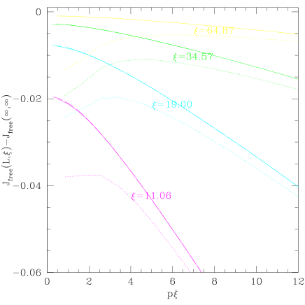
Figure 1: Lattice and finite volume artefacts for the complex free field; dotted curves: $L/\xi\approx 7$, solid lines: $L/\xi\approx 14$, dashed lines: $L/\xi\approx 24$ – the latter two are practically indistinguishable.

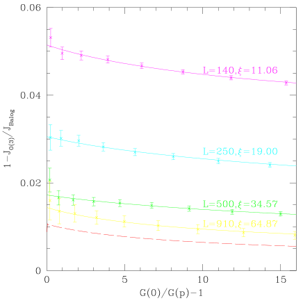
Figure 2: Comparison of Monte-Carlo ($J_{O(3)}$) with form factor results ($J_{ff}$); the dashed line represents the continuum extrapolation.

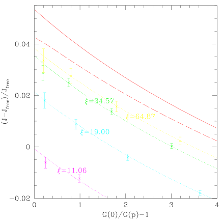
Figure 3: Comparison of Monte-Carlo ($J_{O(3)}$ – dotted lines) and their continuum extrapolation (dashed line) with form factor results ($J_{ff}$ – solid line): interacting contribution.

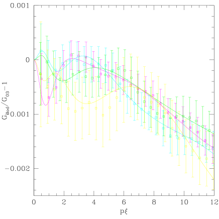
Figure 4: Comparison of $G_{r}$ for $O(3)$ and dodecahedron. Data with $\xi\approx 11,\ 19,\ 34,\ 65$ are overlaid. The solid lines are fits.

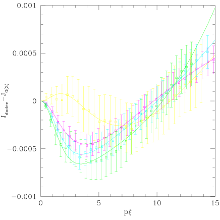
Figure 5: Comparison of $J$ for $O(3)$ and dodecahedron (renormalized). Data with $\xi\approx 11,\ 19,\ 34,\ 65$ are overlaid. The solid lines are fits.

As stated above, our definition of $\xi$ differs from that of Balog and Niedermaier. Even though we could correct for this difference by applying our definition to their data, we decided that a better approach is to eliminate $\xi$ altogether and plot $J$ versus $G(0)/G(p)$. For small $p\xi$ the latter quantity is very close to its free field value, $1+(p\xi)^{2}$. This plot is shown in Fig.2 for various $\xi$ values and $L/\xi$ aproximately 14. The solid lines represent a least square fit to the data of the form

$$\sum_{k=1}^{4}a_{k}(J_{free}(p\xi))^{k}$$ (9)

where

$$J_{free}={1\over 2\pi}-{1\over\pi}\sqrt{1+z/4\over z}\log\Biggl{(}\sqrt{1+{z\over 4}}+\sqrt{{z\over 4}}\Biggr{)}$$ (10)

with $z=(p\xi)^{2}$ is the expression corresponding to $J$ in the free two-component scalar field theory. We also show the extrapolation of our results to the continuum limit using the ansatz in eq.(3) and the form factor prediction. As it can be seen, the latter disagrees with the former.

The disagreement is statistically significant, yet very small. One may wonder how such a wonderful agreement could occur if the form factor prediction is actually false. A possible answer is this: the correlation functions $J$ and $G_{r}$ are, especially at low momenta, very close to those of the free theory, deviating only by less than 5%. The reason behind this is that the form factor squares contributing to the spectral functions of the correlation functions are at low momenta

• dominated by the lowest possible number of intermediate particles (1 for $G_{r}$, 2 for $J$)

• the squares of those lowest form factors are very close (in the case of $G_{r}$ even equal) to those of the free theory.

Therefore, if we want to test the form factor prediction, this universal free field value should be subtracted. To achieve such a subtraction we do the following: we plot $x^{2}J(x)$ versus $G(0)/G(x)$ $x=p\xi$ for both the $O(3)$ model and the free field. We then subtract the two curves at the same value of the abscissa and plot the difference. This is shown in Fig.3, together with the form factor prediction. The latter differs from the continuum value extrapolation by about 25% at $p=0$.

Another quantity which measures directly the nontrivial part of the $S$-matrix is the renormalized coupling $g_{r}$. For the $O(3)$ model this quantity was determined to be around 6.5–6.9 [9] and we determined it again at $\beta=1.5$, $\xi=11.06$ to $g_{r}=6.565(25)$ and at $\beta=1.6$ to $g_{r}=6.609(18)$. Since $g_{r}$ is expected to be monotonically decreasing in $\beta$, the small difference between the two values is probably just due to statistical fluctuations. The value of $g_{r}$ in the form factor approach has not yet been calculated, even though the ingredients are the same as for $G(p)$. We think that the comparison would be most interesting.

Next we would like to present the comparison of the dodecahedron spin model with the $O(3)$ model. If the two models possess the same continuum limit, then one would expect that for sufficiently large $\xi$ both the lattice artefacts and the finite volume corrections become identical. Consequently if we use the same definition for $\xi$ in both models, it should be legitimate to compare the same ‘renormalization group invariants’ at the same $p\xi$ value. In Fig.4 we present the comparison of $G_{r}$. The data are consistent with the hypothesis that the two models have the same continuum limit. The error bars are dominated by the those coming from the dodecahedron, where the fluctuations are very large. We present a similar comparison in Fig.4 for $J$, where the renormalization was chosen so that the rms deviation between the two models in the range from $p\xi=0$ to $p\xi=15$ is minimized. As stated above, the theoretical status of this procedure is not clear. Finally we report on $g_{r}$ for the dodecahdron. We measured it at $\xi=11$ and 19 and obtained 6.42(84) and 6.33(83). These values suggest that its continuum limit value is also around 6.5, in agreement with the value of $g_{r}$ for $O(3)$.

Our conclusion is that whereas there is good numerical evidence that the model defined via the form factor approach does not agree with the continuum limit of the lattice $O(3)$ model, there is no evidence that this limit is different from that of the dodecahedron model. These facts represent a major setback for the accepted saga regarding the special properties of the nonlinear $\sigma$ models with $N\geq 3$.

We acknowledge numerous discussions with J.Balog and M.Niedermaier. A.P. is grateful to the Max-Planck-Institut for its hospitality.

Tab.1:
Susceptibility $\chi$ and effective correlation length $\xi$ for $O(3)$

$\beta$	$L$	# of runs	$\xi$	$\chi$
1.5	$140$	$149$	11.0600(29)	176.7348(566)
1.6	$250$	$86$	18.9971(55)	448.3651(1515)
1.7	$500$	$100$	34.5712(97)	1270.8185(4196)
1.8	$910$	$44$	64.8723(277)	3839.8609(2.1498)

Tab.2:
Susceptibility $\chi$ and effective correlation length $\xi$ for the dodecahedron

$\beta$	$L$	# of runs	$\xi$	$\chi$
1.49	$140$	$246$	11.0540(40)	176.7967(840)
1.5835	$250$	$201$	19.0337(55)	451.1633(2320)
1.672	$500$	$139$	34.4139(167)	1265.2500(7350)
1.76	$910$	$78$	66.6195(522)	4046.1542(3.9885)

References

- [1] A.Patrascioiu and E.Seiler, Phys. Lett. B 430 (1998) 314.
- [2] J.Balog and M.Niedermaier, Phys. Lett. B 386 (1996) 224.
- [3] J.Balog and M.Niedermaier, Nucl. Phys. B 500 (1997) 421.
- [4] J.Balog and M.Niedermaier, Phys.Rev.Lett. 78 (1997) 4151.
- [5] A.Patrascioiu and E.Seiler, Phys.Rev.Lett. 80 (1998) 639.
- [6] U.Wolff, Phys.Rev.Lett. 62 (1989) 361.
- [7] A.Patrascioiu and E.Seiler, Phys.Lett.B 417 (1998) 123.
- [8] A.Patrascioiu and E.Seiler, Phys.Rev. E 57 (1998) 111.
- [9] A.Patrascioiu and E.Seiler, Nuovo Cim. 107A (1994) 765.