The Auxiliary Field Method as a Powerful Tool
for Nonperturbative Study

Abstract

The auxiliary field method, defined through introducing an auxiliary (also called as the Hubbard-Stratonovich or the Mean-) field and utilizing a loop-expansion, gives an excellent result for a wide range of a coupling constant. The analysis is made for Anharmonic-Oscillator and Double-Well examples in 0-(a simple integral) and 1-(quantum mechanics)dimension. It is shown that the result becomes more and more accurate by taking a higher loop into account in a weak coupling region, however, it is not the case in a strong coupling region. The 2-loop approximation is shown to be still insufficient for the Double-Well case in quantum mechanics.

1 Introduction

In most of actual situations, path integral expressions are given as a non-gaussian form so that some approximation is always needed. Apart from perturbative treatment, such as a weak(strong) coupling expansion, which can only describe a small (large) coupling region, we have sought for other recipes to be able to handle cases for a wider coupling range: the variational method[1] has been well known and applied successfully to the polaron problem[2]. The method is combined with an optimization technique and has been actively discussed[3]. Numerical estimation is also possible once expressed in the path integral form: for instance, computer simulations produce a lot of fruitful results such as in Lattice QCD[4], but, in addition to the consumption of money (as well as time), there still lacks something to put symmetry onto the lattice; chiral symmetry is a well-known example[5]. An advantage in path integration, contrary to the operator formalism, is that we can easily switch from one variable to other by means of some change of variables, which would open a new possibility. The auxiliary field is considered as one of these variables, and was introduced into the model by Gross and Neveu[6].

The Gross-Neveu model is a two-dimensional four-fermion model inspired by the work by Nambu and Jona-Lasinio[7];

$${\cal L}=\overline{\psi}i{\partial/}\psi+{g^{2}\over 2}\left(\overline{\psi}\psi\right)^{2}\ ,$$ (1)

where $\psi$ has an $N$-component. After some discussions, they proposed an equivalent Lagrangian,

$${\cal L^{\prime}}=\overline{\psi}i{\partial/}\psi-{\sigma^{2}\over 2}-g\overline{\psi}\psi\sigma\ .$$ (2)

Here $\sigma$ has no kinetic term and is eliminated by using the equation of motion yielding to the original Lagrangian eq.(1). In this sense, we call $\sigma$ as an auxiliary field.

The scenario is more easily understood by means of path integral[8]: the partition function (in an imaginary temperature) reads

$$Z\equiv\int{\cal D}\psi{\cal D}\overline{\psi}\exp\left[i\int d^{2}x\left(\overline{\psi}i{\partial/}\psi+{g^{2}\over 2}\left(\overline{\psi}\psi\right)^{2}\right)\right]\ .$$ (3)

Here introducing the auxiliary field $\sigma$ in terms of the Gaussian integrals, such that

$$1=\int{\cal D}\sigma\exp\left[-i\int d^{2}x{1\over 2}\left(\sigma+g\overline{\psi}\psi\right)^{2}\right]\ ,$$ (4)

and inserting into eq.(3) we find

$$Z=\int\!d\sigma{\cal D}\psi{\cal D}\overline{\psi}\ e^{i\int d^{2}x{\cal L^{\prime}}}=\int\!d\sigma{\cal D}\psi{\cal D}\overline{\psi}\exp\!\left[i\int d^{2}x\left(\overline{\psi}i{\partial/}\psi-{\sigma^{2}\over 2}-g\overline{\psi}\psi\sigma\right)\right]\ .$$ (5)

Similar techniques are utilized everywhere nowadays also for a boson quartic interaction[9] instead of the four-fermi interaction. The nomenclature for $\sigma$-field is, therefore, various; the mean-field[10], the Hubbard-Stratonovich field[11] in solid state physics.

In the actual case, we treat the partition function (which can be obtained through $t\mapsto it$):

$$Z(T)\equiv\int\!d\sigma{\cal D}\psi{\cal D}\overline{\psi}\exp\!\left[-\int_{0}^{T}dt\int dx\left(\overline{\psi}{\partial/}\psi+{\sigma^{2}\over 2}+g\overline{\psi}\psi\sigma\right)\right]\ ,$$ (6)

where the anti-periodic boundary condition for the fermi field, $\psi(T,x)=-\psi(0,x)$, should be understood. We then integrate out the fermion field to find

$$\begin{array}[]{c}\displaystyle{Z(T)=\int\!d\sigma\exp\!\left[-\int d^{2}x{\sigma^{2}\over 2}+N\ln\det\left({\partial/}+g\sigma\right)\right]\equiv\int\!d\sigma e^{-S[\sigma]}\ ,}\\ \vspace{1ex}\cr\displaystyle{S[\sigma]\equiv\int d^{2}x{\sigma^{2}\over 2}-N\ln\det\left({\partial/}+g\sigma\right)\ .}\end{array}$$ (7)

Since we look for a vacuum with $T\mapsto\infty$, we should find a constant solution $\sigma_{0}$ in the equation of motion,

$$\left.{\delta S\over\delta\sigma(x)}\right|_{\sigma_{0}}=0\ ,$$ (8)

which gives the gap equation;

$$\sigma_{0}=2Ng^{2}\int{d^{2}k\over(2\pi)^{2}}\ {\sigma_{0}\over k^{2}+(g\sigma_{0})^{2}}\ .$$ (9)

If $\sigma_{0}$ is non-zero then the dynamically symmetry breaking occurs: this is the end of the usual story. Indeed, the recipe is legitimated if the number of fermion species becomes infinite; $N\rightarrow\infty$. However, it is not the case for most of actual situations: $N$ is finite or even $1$. We wish to know “how accurate is it when $N=1$?”, which is one of the motivation of this work.

Moreover there is an alternative motivation: performing the WKB approximation in the Double-Well potential we must follow instanton calculations[12], which however is very cumbersome as well as tedious. The simpler is the better in any approximation: once introduce an auxiliary field we could avoid such troublesome. To clarify these issues, we pick up the case of quartic coupling of bosonic field for simplicity.

The paper is organized as follows: in §II a simple model calculation is performed for the integral expression. Here we realize the importance of the loop-expansion with respect to the auxiliary field(variable) and can find a more accurate result is obtained if taking a higher loop correction into account when the coupling, $g$, is small. However, when $g$ goes larger, higher loops cannot always improve a situation. We then proceed to the quantum mechanical model in §III, where we compare our results with those obtained numerically to find that the 2-loop correction gives a $4\%$-error for $10^{-3}<g^{2}<10^{3}$ except $g^{2}\sim O\!\left(10^{-1}\right)$ in the Double-Well case. The final section is devoted to a discussion.

2 Simple (0-dimensional) Model

The starting point is

$$I\equiv\int_{-\infty}^{\infty}{dx\over\sqrt{2\pi}}\exp\left[-{\omega^{2}\over 2}x^{2}-{g^{2}\over 8}x^{4}\right]\ .$$ (10)

The integral is expressed as

$$I=\sqrt{\pi|\omega^{2}|\over 4g^{2}}e^{\omega^{4}/4g^{2}}\left\{{\rm I}_{-1/4}\!\left(\!{\omega^{4}\over 4g^{2}}\right)-\epsilon(\omega^{2}){\rm I}_{1/4}\!\left(\!{\omega^{4}\over 4g^{2}}\right)\right\}\ ,$$ (11)

where

$$\epsilon(x)=\left\{\begin{array}[]{c}+1\ :\ x>0\\ -1\ :\ x<0\end{array}\right.\ ,$$

and ${\rm I}_{\alpha}(x)$ is the modified Bessel function. There are two cases depending on a sign $\omega^{2}$:

CASE(i); $\omega^{2}>0$; (0-dimensional Anharmonic-Oscillator),

$$\begin{array}[]{l}\displaystyle{I=\sqrt{\omega^{2}\over 2\pi g^{2}}e^{\omega^{4}/4g^{2}}\ {\rm K}_{1/4}\!\left(\!{\omega^{4}\over 4g^{2}}\right)}\\ \vspace{1ex}\cr\displaystyle{\hskip 4.30554pt\stackrel{{\scriptstyle g^{2}\rightarrow 0}}{{\sim}}1+O(g^{2})\ ;}\end{array}$$ (12)

where ${\rm K}_{\alpha}(x)$ also is the modified Bessel function. And

CASE(ii); $\omega^{2}<0$; (0-dimensional Double-Well),

$$I\stackrel{{\scriptstyle g^{2}\rightarrow 0}}{{\sim}}\sqrt{2}\ e^{\omega^{4}/2g^{2}}\ .$$ (13)

Here it should be noted that $g^{2}=0$ is the essential singularity, that is to say, the Double-Well case is non-Borel summable.

Now introduce an auxiliary field such that

$$1=\int_{-\infty}^{\infty}{dy\over\sqrt{2\pi}}\exp\left[-{1\over 2}\left(y+ig{x^{2}\over 2}\right)^{2}\right]\$$ (14)

so as to erase the $x^{4}$ term when inserted into eq.(10), yielding

$$\begin{array}[]{l}\displaystyle{I=\int_{-\infty}^{\infty}{dx\over\sqrt{2\pi}}{dy\over\sqrt{2\pi}}\exp\left[-{1\over 2}(\omega^{2}+igy)x^{2}-{y^{2}\over 2}\right]}\\ \vspace{1ex}\cr\displaystyle{\hskip 8.61108pt=\int_{-\infty}^{\infty}{dy\over\sqrt{2\pi}}\ (\omega^{2}+igy)^{-1/2}\ e^{-{y^{2}\over 2}}=\int_{-\infty}^{\infty}{dy\over\sqrt{2\pi}}\exp\left[-{y^{2}\over 2}-{1\over 2}\ln\left(\omega^{2}+igy\right)\right]\ .}\end{array}$$ (15)

We rewrite the final expression as

$$\begin{array}[]{c}\displaystyle{I=\int_{-\infty}^{\infty}{dy\over\sqrt{2\pi}}\left.\exp\left[-{S(y)\over a}\right]\right|_{a=1}\ ,}\\ \vspace{1ex}\cr\displaystyle{S(y)\equiv{1\over 2}\ln(\omega^{2}+igy)+{y^{2}\over 2}\ ,}\end{array}$$ (16)

where we have introduced a parameter, $a$, which must be put unity in the final stage. We call $a$ as the loop-expansion parameter. Next, assume the solution of $S^{\prime}(y)=0$ as $y_{{}_{0}}$;

$$S^{\prime}(y)=y+{ig\over 2(\omega^{2}+igy)}=0\ ,$$ (17)

which can be expressed as

$${{\rm\Omega}^{2}-\omega^{2}={g^{2}\over 2{\rm\Omega}^{2}}\ ;}$$ (18)

where ${\rm\Omega}^{2}$ should obey

$${{\rm\Omega}^{2}\equiv\omega^{2}+igy_{{}_{0}}>0\ ;}$$ (19)

since the Gaussian integral of $x$ eq.(15) must exist. Then perform the saddle point method around $y_{{}_{0}}$ to give

$$\begin{array}[]{l}\displaystyle{I=\int_{-\infty}^{\infty}{dy\over\sqrt{2\pi}}\ \exp\!\left[-{S(y_{{}_{0}})\over a}-{S^{(2)}(y_{{}_{0}})\over 2a}(y-y_{{}_{0}})^{2}-{S^{(3)}(y_{{}_{0}})\over 3!a}(y-y_{{}_{0}})^{3}\right.}\\ \vspace{1ex}\cr\displaystyle{\hskip 77.49976pt\left.\left.-{S^{(4)}(y_{{}_{0}})\over 4!a}(y-y_{{}_{0}})^{4}-\cdots\right]\right|_{a=1}\ .}\end{array}$$ (20)

Making a change of variable, $y-y_{{}_{0}}\mapsto y/\sqrt{a}$, we obtain

$$\begin{array}[]{l}\displaystyle{I=e^{-S_{0}/a}\left.\int_{-\infty}^{\infty}\sqrt{a\over 2\pi}\ dy\exp\!\!\left[-{S^{(2)}_{0}\over 2}y^{2}-\sqrt{a}\ {S^{(3)}_{0}\over 3!}y^{3}-a{S^{(4)}_{0}\over 4!}y^{4}-\cdots\right]\right|_{a=1}}\\ \vspace{1ex}\cr\displaystyle{\hskip 8.61108pt\cong\left.e^{-S_{0}/a}\sqrt{a\over 2\pi}\int_{-\infty}^{\infty}dy\ e^{-S^{(2)}_{0}y^{2}/2}\left(1-a\left\{{S^{(4)}_{0}\over 4!}\ y^{4}-{{S^{(3)}_{0}}^{2}\over 2(3!)^{2}}\ y^{6}\right\}+O(a^{2})\right)\right|_{a=1}\ ,}\end{array}$$ (21)

where we have written

$$S^{(n)}\!\left(y_{{}_{0}}\right)\equiv S^{(n)}_{0}\ .$$ (22)

$a^{L-1}$ term is called the $L$-loop term ($L=0$ is the tree term.) From eq.(18),

$${\rm\Omega}^{2}={\omega^{2}+\sqrt{\omega^{4}+2g^{2}}\over 2}\ ,$$ (23)

$$\begin{array}[]{ll}\displaystyle{S_{0}=-{\left({\rm\Omega}^{2}-\omega^{2}\right)^{2}\over 2g^{2}}=-{g^{2}\over 8{\rm\Omega}^{4}}\ ,}&\displaystyle{S_{0}^{(2)}=1+{g^{2}\over 2{\rm\Omega}^{2}}\ ,}\\ \vspace{1ex}\cr\displaystyle{S_{0}^{(3)}=-i{g^{3}\over{\rm\Omega}^{6}}\ ,\quad S_{0}^{(4)}=-3{g^{4}\over{\rm\Omega}^{8}}\ ,}&\displaystyle{S_{0}^{(6)}={5!g^{6}\over 2{\rm\Omega}^{12}}\ .}\end{array}$$ (24)

Using these and performing elementary integrals, we obtain

$$\begin{array}[]{l}\displaystyle{I=\exp\left({g^{2}\over 8{\rm\Omega}^{4}}\right)\sqrt{{\rm\Omega}^{2}\over{\rm\Omega}^{4}+{g^{2}\over 2}}\left(1+{3g^{4}\over 8\left({\rm\Omega}^{4}+{g^{2}\over 2}\right)^{2}}\right.}\\ \vspace{1ex}\cr\displaystyle{\hskip 25.83325pt\left.-{35g^{6}\over 24\left({\rm\Omega}^{4}+{g^{2}\over 2}\right)^{3}}+{329g^{8}\over 128\left({\rm\Omega}^{4}+{g^{2}\over 2}\right)^{4}}-{105g^{10}\over 64\left({\rm\Omega}^{4}+{g^{2}\over 2}\right)^{5}}+O(\mbox{4-loop})\right)\ .}\end{array}$$ (25)

Stated as above, we assign

$$\begin{array}[]{l}\displaystyle{\ I_{\rm tree}\equiv\ \exp\left({g^{2}\over 8{\rm\Omega}^{4}}\right)\ ,}\\ \vspace{1ex}\cr\displaystyle{I_{\rm 1-loop}\equiv I_{\rm tree}\sqrt{{\rm\Omega}^{2}\over{\rm\Omega}^{4}+{g^{2}\over 2}}\ ,}\\ \vspace{1ex}\cr\displaystyle{I_{\rm 2-loop}\equiv I_{\rm 1-loop}\left(1+{3g^{4}\over 8\left({\rm\Omega}^{4}+{g^{2}\over 2}\right)^{2}}-{5g^{6}\over 24\left({\rm\Omega}^{4}+{g^{2}\over 2}\right)^{3}}\right)\ ,}\\ \vspace{1ex}\cr\displaystyle{I_{\rm 3-loop}\equiv\exp\left({g^{2}\over 8{\rm\Omega}^{4}}\right)\sqrt{{\rm\Omega}^{2}\over{\rm\Omega}^{4}+{g^{2}\over 2}}\left(1+{3g^{4}\over 8\left({\rm\Omega}^{4}+{g^{2}\over 2}\right)^{2}}\right.}\\ \vspace{1ex}\cr\displaystyle{\hskip 34.44434pt\left.-{35g^{6}\over 24\left({\rm\Omega}^{4}+{g^{2}\over 2}\right)^{3}}+{329g^{8}\over 128\left({\rm\Omega}^{4}+{g^{2}\over 2}\right)^{4}}-{105g^{10}\over 64\left({\rm\Omega}^{4}+{g^{2}\over 2}\right)^{5}}\right)\ .}\end{array}$$ (26)

Let us analyze the individual case:

• CASE(i); 0-dimensional Anharmonic-Oscillator. Put $\omega^{2}\mapsto 1$ so that eq.(23) reads

  $${\rm\Omega}^{2}={\sqrt{1+2g^{2}}+1\over 2}\ .$$ (27)

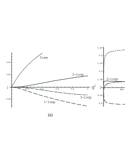
Figure 1: 0-dimensional Anharmonic Case: (a); $g^{2}\leq 1$. (b); $g^{2}>1$. Dotted line: $I_{\rm Tree}/\mbox{Exact}$. Dashed line: $I_{\rm 1-loop}/\mbox{Exact}$. Solid line: $I_{\rm 2-loop}/\mbox{Exact}$. Dash-dotted line: $I_{\rm 3-loop}/\mbox{Exact}$.

  We plot the ratio of $I_{\rm L-loop}$(L=0,1,2,3) to the exact value in Fig.(1). (a) shows the case of $g^{2}\leq 1$ and (b) of $g^{2}>1$. Details are seen in table (a).

$\displaystyle{g^{2}}$	Exact	$\begin{array}[]{c}\mbox{Tree}\\ \mbox{Tree/ Ex.}\end{array}$	$\begin{array}[]{c}\mbox{1-loop}\\ \mbox{1-loop/ Ex.}\end{array}$	$\begin{array}[]{c}\mbox{2-loop}\\ \mbox{2-loop / Ex.}\end{array}$	$\begin{array}[]{c}\mbox{3-loop}\\ \mbox{3-loop / Ex.}\end{array}$
$10^{-3}$	0.9996	$\begin{array}[]{c}0.9999\\ 1.00\end{array}$	$\begin{array}[]{c}0.9996\\ 1.\end{array}$	$\begin{array}[]{c}0.9996\\ 1.\end{array}$	$\begin{array}[]{c}0.9996\\ 1.\end{array}$
$10^{-2}$	0.9963	$\begin{array}[]{c}0.9988\\ 1.00\end{array}$	$\begin{array}[]{c}0.9963\\ 1.\end{array}$	$\begin{array}[]{c}0.9963\\ 1.\end{array}$	$\begin{array}[]{c}0.9963\\ 1.\end{array}$
$10^{-1}$	0.9685	$\begin{array}[]{c}0.9881\\ 1.02\end{array}$	$\begin{array}[]{c}0.9664\\ 1.00\end{array}$	$\begin{array}[]{c}0.9690\\ 1.00\end{array}$	$\begin{array}[]{c}0.9683\\ 1.00\end{array}$
$1$	0.8386	$\begin{array}[]{c}0.9149\\ 1.1\end{array}$	$\begin{array}[]{c}0.8125\\ 0.97\end{array}$	$\begin{array}[]{c}0.8541\\ 1.02\end{array}$	$\begin{array}[]{c}0.8277\\ 0.99\end{array}$
$10$	0.5954	$\begin{array}[]{c}0.7027\\ 1.18\end{array}$	$\begin{array}[]{c}0.5484\\ 0.92\end{array}$	$\begin{array}[]{c}0.6195\\ 1.04\end{array}$	$\begin{array}[]{c}0.5976\\ 1.00\end{array}$
$10^{2}$	0.3672	$\begin{array}[]{c}0.4510\\ 1.23\end{array}$	$\begin{array}[]{c}0.3300\\ 0.90\end{array}$	$\begin{array}[]{c}0.3817\\ 1.04\end{array}$	$\begin{array}[]{c}0.3790\\ 1.03\end{array}$
$10^{3}$	0.2131	$\begin{array}[]{c}0.2656\\ 1.25\end{array}$	$\begin{array}[]{c}0.1899\\ 0.89\end{array}$	$\begin{array}[]{c}0.2210\\ 1.037\end{array}$	$\begin{array}[]{c}0.2222\\ 1.043\end{array}$

table(a)

• CASE (ii); 0-dimensional Double-Well. Put $\omega^{2}\mapsto-1$ so that eq.(23) reads

  $${\rm\Omega}^{2}={\sqrt{1+2g^{2}}-1\over 2}\ .$$ (28)

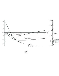
Figure 2: 0-dimensional Double-Well Case: (c); $g^{2}\leq 1$. (d); $g^{2}>1$. Dotted line: $I_{\rm Tree}/\mbox{Exact}$: this is omitted in (c); because of a large deviation. Dashed line: $I_{\rm 1-loop}/\mbox{Exact}$. Solid line: $I_{\rm 2-loop}/\mbox{Exact}$. Dash-dotted line: $I_{\rm 3-loop}/\mbox{Exact}$.

  We plot the same ratio as the above in Fig.(2). However, in (c) we have omitted the tree graph because of the large deviation. Details are shown in table (b).

$\displaystyle{g^{2}}$	Exact	$\begin{array}[]{c}\mbox{Tree}\\ \mbox{Tree/Ex.}\end{array}$	$\begin{array}[]{c}\mbox{1-loop}\\ \mbox{1-loop/Ex.}\end{array}$	$\begin{array}[]{c}\mbox{2-loop}\\ \mbox{2-loop/Ex.}\end{array}$	$\begin{array}[]{c}\mbox{3-loop}\\ \mbox{3-loop/Ex.}\end{array}$
$10^{-3}$	$1.986\!\times\!10^{217}$	$\begin{array}[]{c}1.035\!\times\!10^{219}\\ 52.1\end{array}$	$\begin{array}[]{c}2.313\!\times\!10^{217}\\ 1.17\end{array}$	$\begin{array}[]{c}1.930\!\times\!10^{217}\\ 0.97\end{array}$	$\begin{array}[]{c}1.961\!\times\!10^{217}\\ 0.98\end{array}$
$10^{-2}$	$7.360\!\times\!10^{21}$	$\begin{array}[]{c}1.210\!\times\!10^{23}\\ 16.44\end{array}$	$\begin{array}[]{c}8.495\!\times\!10^{21}\\ 1.15\end{array}$	$\begin{array}[]{c}7.162\!\times\!10^{21}\\ 0.97\end{array}$	$\begin{array}[]{c}7.270\!\times\!10^{21}\\ 0.98\end{array}$
$10^{-1}$	$2.208\!\times\!10^{2}$	$\begin{array}[]{c}1.107\!\times\!10^{3}\\ 5.01\end{array}$	$\begin{array}[]{c}2.311\!\times\!10^{2}\\ 1.05\end{array}$	$\begin{array}[]{c}2.112\!\times\!10^{2}\\ 0.96\end{array}$	$\begin{array}[]{c}2.156\!\times\!10^{2}\\ 0.98\end{array}$
$1$	2.350	$\begin{array}[]{c}4.202\\ 1.79\end{array}$	$\begin{array}[]{c}1.932\\ 0.82\end{array}$	$\begin{array}[]{c}2.155\\ 0.92\end{array}$	$\begin{array}[]{c}2.411\\ 1.03\end{array}$
$10$	0.8074	$\begin{array}[]{c}1.103\\ 1.37\end{array}$	$\begin{array}[]{c}0.6897\\ 0.85\end{array}$	$\begin{array}[]{c}0.8137\\ 1.01\end{array}$	$\begin{array}[]{c}0.8768\\ 1.09\end{array}$
$10^{2}$	0.4040	$\begin{array}[]{c}0.5196\\ 1.29\end{array}$	$\begin{array}[]{c}0.3542\\ 0.88\end{array}$	$\begin{array}[]{c}0.4159\\ 1.03\end{array}$	$\begin{array}[]{c}0.4295\\ 1.06\end{array}$
$10^{3}$	0.2196	$\begin{array}[]{c}0.2777\\ 1.26\end{array}$	$\begin{array}[]{c}0.1942\\ 0.88\end{array}$	$\begin{array}[]{c}0.2270\\ 1.03\end{array}$	$\begin{array}[]{c}0.2312\\ 1.05\end{array}$

table(b)

From the figures, (1) and (2), it should be noted that the higher loop corrections improve the result all the time when $g^{2}\leq 1$ but not in the strong coupling region as is seen from the graphs (b) and (d). Details for the values are listed in the tables (a) and (b). This fact implies that the loop-expansion is merely an asymptotic expansion. In the Anharmonic Oscillator case, especially the result is satisfactory: the 2-loop result gives a 4%-error for $10^{-3}<g^{2}<10^{3}$. In the Double-Well case, the 3-loop spoils the result at $1<g^{2}$ but gives a better result at $g^{2}<1$. However, it is still remarkable that the error, under the 2-loop, remains within $\sim 8\%$ for a huge coupling region, $10^{-3}<g^{2}<10^{3}$.

The essential role of the loop-expansion should finally be remarked: if we stop at the $g^{4}$ term in the 2- or 3-loop expression eq.(26), the result deviates far away from the true value. Therefore we must abandon the coupling constant expansion in the auxiliary field method.

3 The Quantum Mechanical Model

Encouraged by the foregoing results, in this section we analyze the quantum mechanical model:

$$H={p^{2}\over 2}+{\omega^{2}\over 2}x^{2}+{g^{2}\over 8}x^{4}\ .$$ (29)

Here again cases are classified into (i) $\omega^{2}>0$; Anharmonic-Oscillator. And (ii) $\omega^{2}<0$; Double-Well. The partition function is given by

$$\begin{array}[]{l}\displaystyle{Z(T)={\rm Tr}\ e^{-TH}}\\ \vspace{1ex}\cr\displaystyle{\hskip 25.83325pt=\int{\cal D}x\exp\left.\left[-\int_{0}^{T}\!\!dt\left({{\dot{x}}^{2}\over 2}+{\omega^{2}\over 2}x^{2}+{g^{2}\over 8}x^{4}\right)\right]\right|_{x(T)=x(0)}\ ,}\end{array}$$ (30)

where $x(T)=x(0)$ designates the periodic boundary condition. Here and hereafter we put $\hbar\mapsto 1$ and use the continuous representation,

$${\cal D}x\equiv\lim_{N\rightarrow\infty}\prod_{j=1}^{N}{dx_{j}\over\sqrt{2\pi\Delta t}}\ ;\qquad\Delta t\equiv{T\over N}\ .$$ (31)

Introducing an auxiliary field in terms of the Gaussian identity,

$$1=\int{\cal D}y\exp\!\left[-\int_{0}^{T}\!\!dt\ {1\over 2}\left(y+{igx^{2}\over 2}\right)^{2}\right]\ ,$$ (32)

so as to erase the quartic term, we obtain

$$Z(T)=\int\!{\cal D}x{\cal D}y\exp\!\left[-\!\int_{0}^{T}\!\!dt\!\left({{\dot{x}}^{2}\over 2}+\left(\!\omega^{2}\!+igy\right){x^{2}\over 2}+{y^{2}\over 2}\right)\!\right]\ ,$$ (33)

which becomes, after the integration with respect to $x$, to

$$\begin{array}[]{c}\displaystyle{Z(T)=\int\!\!{\cal D}y\exp\!\left[\!-\int_{0}^{T}\!\!dt\ {y^{2}\over 2}+{1\over 2}\ln\det\!\left(\!-{d^{2}\over dt^{2}}+\!\omega^{2}\!+igy\!\right)\right]}\\ \vspace{1ex}\cr\displaystyle{\equiv\int\!\!{\cal D}y\left.\exp\!\left(-{S[y]\over a}\right)\right|_{a=1}\ ,}\end{array}$$ (34)

where

$$S[y]\equiv\int_{0}^{T}\!\!dt\ {y^{2}\over 2}+{1\over 2}\ln\det\!\left(\!-{d^{2}\over dt^{2}}+\!\omega^{2}\!+igy\!\right)\ ,$$ (35)

and again the loop-expansion parameter,$a$, has been introduced.

Write a solution of the equation of motion, $S^{\prime}[y]=\delta S[y]/\delta y(t)=0$, ${y}_{{}_{0}}(t)$, giving the gap equation;

$${y}_{{}_{0}}(t)+{ig\over 2}G(t,t)=0\ ,$$ (36)

which can be rewritten as

$${{\rm\Omega}(t)}^{2}-\omega^{2}={g^{2}\over 2}G(t,t)\ ,$$ (37)

where

$${\rm\Omega}(t)^{2}\equiv\omega^{2}+ig{y}_{{}_{0}}(t)\ .$$ (38)

Here the Green’s function,$G(t,t^{\prime})$, obeys

$$\left(-{d^{2}\over dt^{2}}+{\rm\Omega}(t)^{2}\right)G(t,t^{\prime})=\delta(t-t^{\prime})\ .$$ (39)

Again it should be noted that

$${\rm\Omega}(t)^{2}>0\ ,$$ (40)

due to the existence of the Gaussian integration of $x$ in eq.(33).

Now $S[y]$ is expanded around ${y}_{{}_{0}}$ (or ${\rm\Omega}(t)^{2}$) such that

$$S[y]=S_{0}+{1\over 2}(y-{y}_{{}_{0}})^{2}\cdot S^{(2)}_{0}+{1\over 3!}(y-{y}_{{}_{0}})^{3}\cdot S^{(3)}_{0}+\cdots\ ,$$ (41)

where abbreviations

$$S^{(n)}_{0}\equiv\left.{\delta^{n}S\over\delta y(t_{1})\delta y(t_{2})\cdots\delta y(t_{n})}\right|_{y={y}_{{}_{0}}}\ ,$$ (42)

and

$$\begin{array}[]{l}\displaystyle{(y-{y}_{{}_{0}})^{n}\cdot S^{(n)}_{0}}\\ \vspace{1ex}\cr\displaystyle{\equiv\int dt_{1}dt_{2}\cdots dt_{n}(y-{y}_{{}_{0}})(t_{1})(y-{y}_{{}_{0}})(t_{2})\cdots(y-{y}_{{}_{0}})(t_{n})\left.{\delta^{n}S\over\delta y(t_{1})\delta y(t_{2})\cdots\delta y(t_{n})}\right|_{y={y}_{{}_{0}}}\ ,}\end{array}$$ (43)

have been adopted. Shifting and scaling the integration variables as before, we obtain

$$Z(T)=e^{-S_{0}/a}\left.\int\!{\cal D}y\exp\!\left[-{1\over 2}\Delta^{-1}\cdot y^{2}-\sqrt{a}\ {y^{3}\over 3!}\cdot S^{(3)}_{0}-a\ {y^{4}\over 4!}\cdot S^{(4)}_{0}-\cdots\right]\right|_{a=1}\ ,$$ (44)

where we have written $S^{(2)}_{0}\mapsto\Delta^{-1}$ which reads explicitly

$$\Delta^{-1}(t_{1},t_{2})\equiv\left.{\delta^{2}S\over\delta y(t_{1})\delta y(t_{2})}\right|_{y={y}_{{}_{0}}}=\delta(t_{1}-t_{2})+{g^{2}\over 2}G(t_{1},t_{2})G(t_{2},t_{1})\ .$$ (45)

Moreover,

$$\begin{array}[]{l}\displaystyle{S^{(3)}_{0}=-{ig^{3}\over 2}\Bigg{\{}G(t_{1},t_{2})G(t_{2},t_{3})G(t_{3},t_{1})+G(t_{1},t_{3})G(t_{3},t_{2})G(t_{2},t_{1})\Bigg{\}}\ ,}\\ \vspace{1ex}\cr\displaystyle{S^{(4)}_{0}=-g^{4}\Bigg{\{}G(t_{1},t_{2})G(t_{2},t_{3})G(t_{3},t_{4})G(t_{4},t_{1})+G(t_{1},t_{2})G(t_{2},t_{4})G(t_{4},t_{3})G(t_{3},t_{1})}\\ \vspace{1ex}\cr\displaystyle{\hskip 107.63855pt+G(t_{1},t_{3})G(t_{3},t_{2})G(t_{2},t_{4})G(t_{4},t_{1})\Bigg{\}}\ .}\end{array}$$ (46)

From these we have

$$\begin{array}[]{l}\displaystyle{{Z(T)}_{{\rm Tree}}\equiv\exp\left(-S_{0}\right)\ ,}\\ \vspace{1ex}\cr\displaystyle{{Z(T)}_{{\rm 1-loop}}\equiv\exp\left(-S_{0}-{1\over 2}\ln\det\Delta\right)\ ,}\\ \vspace{1ex}\cr\displaystyle{{Z(T)}_{{\rm 2-loop}}\equiv\exp\left(-S_{0}-{1\over 2}\ln\det\Delta\right)\times\Big{[}1+(\mbox{2-loop Graphs})\Big{]}\ ,}\end{array}$$ (47)

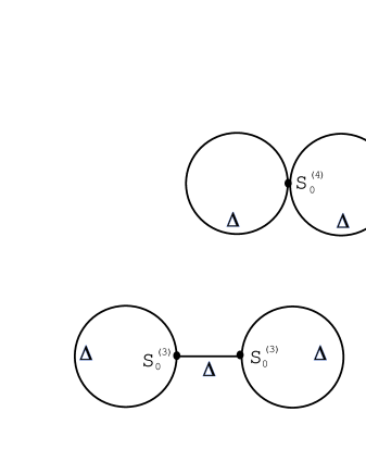
Figure 3: Formal 2-loop Graphs: $\Delta$ denotes the propagator of the auxiliary field.

where the 2-loop graphs are formally given by Fig.(3).

Therefore the rest of the work is to fix the form of the Green’s function eq.(39) and find the solution ${y}_{{}_{0}}(t)$ of the gap equation eq.(37). In this paper we confine ourselves to a time-independent solution: those quantities obtained so far turn into the overlined ones;

$${y}_{{}_{0}}(t)\mapsto\overline{{y}_{{}_{0}}}:\mbox{constant}\ ;\quad{\rm\Omega}(t)^{2}\mapsto\overline{{\rm\Omega}}^{2}:\mbox{constant}\ .$$ (48)

The Green’s function eq.(39) can be obtained explicitly

$$\begin{array}[]{l}\displaystyle{\overline{G}(t,t^{\prime};\overline{{\rm\Omega}})\equiv{1\over T}\!\sum_{r=-\infty}^{\infty}\!{e^{i2\pi r(t-t^{\prime})/T}\over\left({2\pi r\over T}\right)^{2}+\overline{{\rm\Omega}}^{2}}}\\ \vspace{1ex}\cr\displaystyle{={1\over 2\overline{{\rm\Omega}}\sinh{\overline{{\rm\Omega}}T\over 2}}\left\{\theta(t-t^{\prime})\cosh\overline{{\rm\Omega}}\left({T\over 2}-t+t^{\prime}\right)+\theta(t^{\prime}-t)\cosh\overline{{\rm\Omega}}\left({T\over 2}+t-t^{\prime}\right)\right\}\ ,}\end{array}$$ (49)

where we have taken the periodic boundary condition into account.

Now $\overline{{\rm\Omega}}$ is the solution of the gap equation;

$$ig\overline{{y}_{{}_{0}}}=\overline{{\rm\Omega}}^{2}-\omega^{2}={g^{2}\over 2}\overline{G}\!\left(t,t;\overline{{\rm\Omega}}\!\right)={g^{2}\over 4\overline{{\rm\Omega}}}\coth\left({\overline{{\rm\Omega}}T\over 2}\right)\ .$$ (50)

When $T\rightarrow$ large, $\overline{{\rm\Omega}}$ can be expressed as

$$\overline{{\rm\Omega}}={\rm\Omega}_{0}+{\rm\Omega}_{1}e^{-{\rm\Omega}_{0}T}+{\rm\Omega}_{2}e^{-2{\rm\Omega}_{0}T}+\cdots\ ,$$ (51)

where ${\rm\Omega}_{0}$ is the solution of the third degree equation;

$${\rm\Omega}_{0}^{3}-\omega^{2}{\rm\Omega}_{0}={g^{2}\over 4}\ .$$ (52)

(In order to calculate the energy of the first excited state, ${\rm\Omega}_{1}$ must be known, which is easily obtained to be

$${\rm\Omega}_{1}={g^{2}\over 2\left(3{\rm\Omega}_{0}^{2}+\omega^{2}\right)}\ .$$ (53)

In this paper, however, only the ground state energy is considered.) Other overlined quantities are found straightforwardly; especially

$$\overline{\Delta}(t,t^{\prime})=\left(\left.{\delta^{2}S\over\delta y(t)\delta y(t^{\prime})}\right|_{y=\overline{{y}_{{}_{0}}}}\right)^{-1}=\delta(t-t^{\prime})-{g^{2}\over 2\overline{{\rm\Omega}}}\overline{G}\!\left(t,t^{\prime};\hat{\rm\Omega}\right)\ ,$$ (54)

where

$${\hat{\rm\Omega}}^{2}\equiv 4\overline{{\rm\Omega}}^{2}+{g^{2}\over 2\overline{{\rm\Omega}}}\ .$$ (55)

The tree part in eq.(47) becomes

$${\overline{Z}(T)}_{{\rm Tree}}\equiv\exp\left(-\overline{S_{0}}\right)\ ,$$ (56)

with

$$\begin{array}[]{l}\displaystyle{\overline{S_{0}}=T\ {{\overline{{y}_{{}_{0}}}}^{2}\over 2}+{1\over 2}\sum_{r=-\infty}^{\infty}\ln\left\{\left({2\pi r\over T}\right)^{2}+{\overline{\rm\Omega}}^{2}\right\}}\\ \vspace{1ex}\cr\displaystyle{\hskip 12.91663pt=-{T\over 2g^{2}}\left({\overline{\rm\Omega}}^{2}-\omega^{2}\right)^{2}+\ln\sinh\left({\overline{\rm\Omega}T\over 2}\right)+\left(\mbox{$\overline{\rm\Omega}$-independent part}\right)\ ,}\end{array}$$ (57)

where the gap equation eq.(50) has been utilized to the first term in the final expression. In the 1-loop part of eq.(47), we should know $\ln\det\overline{\Delta}(t,t^{\prime})$ which is

$$\begin{array}[]{l}\displaystyle{{1\over 2}\ln\det\overline{\Delta}(t,t^{\prime})={1\over 2}\sum_{r=-\infty}^{\infty}\ln\left\{1+{g^{2}T^{2}\over 8\pi^{2}\overline{\rm\Omega}}\ {1\over r^{2}+\left(\overline{\rm\Omega}T/\pi\right)^{2}}\right\}}\\ \vskip 4.30554pt\cr\displaystyle{={1\over 2}\sum_{r=-\infty}^{\infty}\left\{\ln\Big{[}r^{2}+\left({\hat{\rm\Omega}T\over 2\pi}\right)^{2}\Big{]}-\ln\Big{[}r^{2}+\left({\overline{\rm\Omega}T\over\pi}\right)^{2}\Big{]}\right\}=\ln\left({\sinh\left(\hat{\rm\Omega}T/2\right)\over\sinh\left(\overline{\rm\Omega}T\right)}\right)\ .}\end{array}$$ (58)

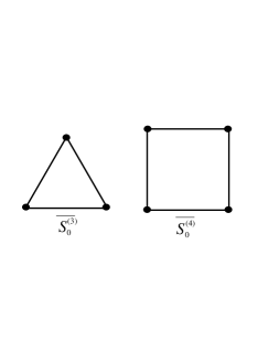
Figure 4: Vertices for the constant classical solution: the solid line represents $\overline{G}\!\left(t,t^{\prime};\overline{\rm\Omega}\right)$ and the dot represents the vertex which should be attached by the double-lined $\overline{\Delta}(t,t^{\prime})$.

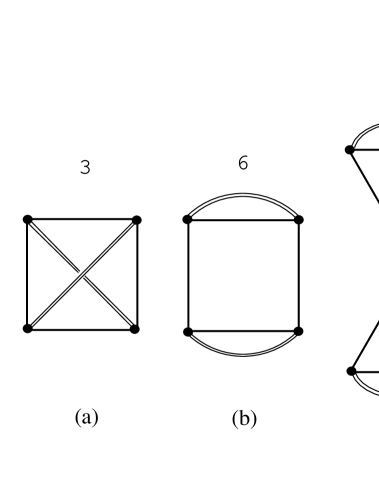
Figure 5: The 2-loop Graphs for the constant classical solution: the upper numbers in the figures represent those of multiplicity.

As for the 2-loop part, the (non-local) vertices $\overline{S_{0}^{(3)}}$ and $\overline{S_{0}^{(4)}}$ are now expressed as in Fig.(4). Accordingly, the 2-loop part is written as in Fig.(5):

From the graphs, we should note that there need, in the ordinary sense, the 3- and 4-loop calculations in the 2-loop of the auxiliary field, since our vertices, $\overline{S_{0}^{(3)}}$ and $\overline{S_{0}^{(4)}}$, are non-local. Due to this complexity, we confine ourselves to the case that $T\mapsto\infty$, that is, to the ground state. Write the Fourier transformed $\overline{G}$ and $\overline{\Delta}$ as

$$\begin{array}[]{l}\displaystyle{\overline{G}\!\left(t,t^{\prime};{\rm\Omega}_{0}\right)=\int_{-\infty}^{\infty}{dk\over 2\pi}e^{-ik(t-t^{\prime})}{1\over k^{2}+{\rm\Omega}_{0}^{2}}\equiv\int_{-\infty}^{\infty}{dk\over 2\pi}e^{-ik(t-t^{\prime})}G_{0}(k)\ ,}\\ \vspace{1ex}\cr\displaystyle{\overline{\Delta}(t,t^{\prime})=\int_{-\infty}^{\infty}{dk\over 2\pi}e^{-ik(t-t^{\prime})}{k^{2}+4{\rm\Omega}^{2}_{0}\over k^{2}+{\hat{\rm\Omega}}^{2}}\equiv\int_{-\infty}^{\infty}{dk\over 2\pi}e^{-ik(t-t^{\prime})}\Delta_{0}(k)\ ,}\end{array}$$ (59)

where

$${\hat{\rm\Omega}}^{2}\equiv 4{\rm\Omega}_{0}^{2}+{g^{2}\over 2{\rm\Omega}_{0}}\ ;$$ (60)

since $\overline{\rm\Omega}$ is now ${\rm\Omega}_{0}$ under $T\rightarrow\infty$. With these, each graph, (a) $\sim$ (d), can be expressed and calculated elementally as follows:

(a) $$= {g^{4}\over 8}\int{dl\,dp\,dk\over(2\pi)^{3}}\,\Delta_{0}(p)\Delta_{0}(k)G_{0}(l)G_{0}(l+k)G_{0}(l+p)G_{0}(l+k+p)$$

$$= {g^{4}\over 64{\rm\Omega}_{0}^{5}}{\rho+10\over\rho^{2}(\rho+1)(\rho+2)}\ .$$

(b) $$= {g^{4}\over 4}\int{dl\,dp\,dk\over(2\pi)^{3}}\,\Delta_{0}(p)\Delta_{0}(k)G_{0}(l)^{2}G_{0}(l+k)G_{0}(l+p)={g^{4}\over 64{\rm\Omega}_{0}^{5}}{\rho+10\over\rho^{2}(\rho+1)}\ .$$ (62)

(c) $$= -{g^{6}\over 8}\Delta_{0}(0)\left[\int{dl\,dp\over(2\pi)^{2}}\,\Delta_{0}(p)G_{0}(l)^{2}G_{0}(l+p)\right]^{2}=-{g^{6}\over 128{\rm\Omega}_{0}^{8}}{(\rho+6)^{2}\over\rho^{4}(\rho+2)^{2}}\ .$$ (63)

(d) $$= -{g^{6}\over 12}\int{dl\,dp\,dk\,dq\over(2\pi)^{4}}\,\Delta_{0}(p)\Delta_{0}(q)\Delta_{0}(p+q)$$

$$\times G_{0}(l)G_{0}(l+p)G_{0}(l+p+q)G_{0}(k)G_{0}(k+q)G_{0}(k+q+p)$$

$$= -{g^{6}\over 64{\rm\Omega}_{0}^{8}}{(\rho^{2}+8\rho+4)\over\rho^{4}(\rho+1)(\rho+2)^{2}}\ .$$

Here we have introduced a parameter,

$$\rho\equiv\sqrt{{\hat{\rm\Omega}}^{2}\over{\rm\Omega}_{0}^{2}}\ .$$ (65)

The result for the ground state energy,

$$E_{0}=-\lim_{T\rightarrow\infty}\ {1\over T}\ln Z(T)\ ,$$ (66)

is therefore

$$E_{0}^{\rm tree} = {{\rm\Omega}_{0}\over 2}-{g^{2}\over 32{\rm\Omega}_{0}^{2}}\ ,$$ (67)

$$E_{0}^{1-{\rm loop}} = {{\rm\Omega}_{0}\over 2}\left(\rho-1\right)-{g^{2}\over 32{\rm\Omega}_{0}^{2}}\ ,$$ (68)

$$E_{0}^{2-{\rm loop}} = {{\rm\Omega}_{0}\over 2}\left(\rho-1\right)-{g^{2}\over 32{\rm\Omega}_{0}^{2}}-\ {g^{4}\over 64{\rm\Omega}_{0}^{5}}\ {(\rho+3)(\rho+10)\over\rho^{2}(\rho+1)(\rho+2)}$$

$$\hskip 17.22217pt+\ {g^{6}\over 128{\rm\Omega}_{0}^{8}}\ {\rho^{3}+15\rho^{2}+64\rho+44\over\rho^{4}(\rho+1)(\rho+2)^{2}}\ .$$

Let us analyze the individual case:

• CASE(i); Anharmonic-Oscillator. The solution of eq.(52) is given[13] by

  $${\rm\Omega}_{0}=\left\{\!\!\begin{array}[]{c c}\displaystyle{{2\omega\over\sqrt{3}}\cos\Bigl{[}{1\over 3}\cos^{-1}\left({3\sqrt{3}g^{2}\over 8\omega^{3}}\right)\Bigr{]}}&\displaystyle{:\ 0\leq{g^{2}\over 8}\leq{\omega^{3}\over 3\sqrt{3}}}\\ \vskip 8.61108pt\cr\displaystyle{\sqrt[3]{{g^{2}\over 8}+\sqrt{{g^{4}\over 64}-{\omega^{6}\over 27}}}+\sqrt[3]{{g^{2}\over 8}-\sqrt{{g^{4}\over 64}-{\omega^{6}\over 27}}}}&\displaystyle{:\ {\omega^{3}\over 3\sqrt{3}}\leq{g^{2}\over 8}}\end{array}\right.$$ (70)

  Putting $\omega^{2}\mapsto 1$ we calculate the ratio of $E_{0}^{\rm L-loop}$(L=0,1,2) to the exact numerical value in table (c).

$\displaystyle{g^{2}/8}$	Exact	$\begin{array}[]{c}\mbox{Tree}\\ \mbox{Tree/ Ex.}\end{array}$	$\begin{array}[]{c}\mbox{1-loop}\\ \!\!\mbox{1-loop/ Ex.}\!\!\end{array}$	$\begin{array}[]{c}\mbox{2-loop}\\ \!\!\mbox{2-loop / Ex.}\!\!\end{array}$
$10^{-3}$	0.50075	$\begin{array}[]{c}0.50025\\ 0.9990\end{array}$	$\begin{array}[]{c}0.50075\\ 1.\end{array}$	$\begin{array}[]{c}0.50075\\ 1.\end{array}$
$10^{-2}$	0.50726	$\begin{array}[]{c}0.50248\\ 0.9906\end{array}$	$\begin{array}[]{c}0.50737\\ 1.0002\end{array}$	$\begin{array}[]{c}0.50725\\ 0.9999\end{array}$
$10^{-1}$	0.55915	$\begin{array}[]{c}0.52290\\ 0.9352\end{array}$	$\begin{array}[]{c}0.56435\\ 1.009\end{array}$	$\begin{array}[]{c}0.55775\\ 0.9975\end{array}$
$1$	0.80377	$\begin{array}[]{c}0.65268\\ 0.8038\end{array}$	$\begin{array}[]{c}0.85522\\ 1.0640\end{array}$	$\begin{array}[]{c}0.78548\\ 0.9772\end{array}$
$10$	1.5050	$\begin{array}[]{c}1.1080\\ 0.7362\end{array}$	$\begin{array}[]{c}1.6729\\ 1.1116\end{array}$	$\begin{array}[]{c}1.4738\\ 0.9793\end{array}$
$10^{2}$	3.1314	$\begin{array}[]{c}2.2356\\ 0.7139\end{array}$	$\begin{array}[]{c}3.5280\\ 1.1267\end{array}$	$\begin{array}[]{c}3.0865\\ 0.9857\end{array}$
$10^{3}$	6.6942	$\begin{array}[]{c}4.7445\\ 0.7088\end{array}$	$\begin{array}[]{c}7.5659\\ 1.1302\end{array}$	$\begin{array}[]{c}6.6112\\ 0.9876\end{array}$

table(c)

• CASE(ii); Double-Well. The solution of eq.(52) is

  $${\rm\Omega}_{0}=\sqrt[3]{\sqrt{{g^{4}\over 64}+{\left|\omega^{2}\right|^{3}\over 27}}+{g^{2}\over 8}}-\sqrt[3]{\sqrt{{g^{4}\over 64}+{\left|\omega^{2}\right|^{3}\over 27}}-{g^{2}\over 8}}\ .$$ (71)

  Putting $\omega^{2}\mapsto-1$ we again compare the result to the exact numerical value in table (d).

$\displaystyle{g^{2}/8}$	Exact	$\begin{array}[]{c}\mbox{Tree}\\ \mbox{Tree/ Ex.}\end{array}$	$\begin{array}[]{c}\mbox{1-loop}\\ \mbox{1-loop/ Ex.}\end{array}$	$\begin{array}[]{c}\mbox{2-loop}\\ \mbox{2-loop / Ex.}\end{array}$
$10^{-3}$	-61.794	$\begin{array}[]{c}-62.500\\ 1.0114\end{array}$	$\begin{array}[]{c}-61.794\\ 1.\end{array}$	$\begin{array}[]{c}-61.794\\ 1.\end{array}$
$10^{-2}$	-5.5532	$\begin{array}[]{c}-6.245\\ 1.1246\end{array}$	$\begin{array}[]{c}-5.5575\\ 1.0008\end{array}$	$\begin{array}[]{c}-5.5541\\ 1.0002\end{array}$
$10^{-1}$	-0.15413	$\begin{array}[]{c}-0.57593\\ 3.7368\end{array}$	$\begin{array}[]{c}-0.02326\\ 0.1509\end{array}$	$\begin{array}[]{c}-0.08479\\ 0.5501\end{array}$
$1$	0.51478	$\begin{array}[]{c}0.25\\ 0.4856\end{array}$	$\begin{array}[]{c}0.66421\\ 1.2903\end{array}$	$\begin{array}[]{c}0.41605\\ 0.8082\end{array}$
$10$	1.3716	$\begin{array}[]{c}0.92366\\ 0.6734\end{array}$	$\begin{array}[]{c}1.5839\\ 1.1548\end{array}$	$\begin{array}[]{c}1.2112\\ 0.8830\end{array}$
$10^{2}$	3.0695	$\begin{array}[]{c}2.1501\\ 0.7005\end{array}$	$\begin{array}[]{c}3.4867\\ 1.1359\end{array}$	$\begin{array}[]{c}2.7543\\ 0.8973\end{array}$
$10^{3}$	6.6655	$\begin{array}[]{c}4.7048\\ 0.7059\end{array}$	$\begin{array}[]{c}7.5467\\ 1.1322\end{array}$	$\begin{array}[]{c}6.0004\\ 0.9002\end{array}$

table(d)

From the above tables, in case (i) the auxiliary field method can fit the data within a 13%-error under the 1-loop and a 3%-error under the 2-loop, which is considered to be excellent. For the Double-Well case, the method gives us $\sim 10\%$- error except the region, $O\!\left(10^{-2}\right)<g^{2}<O(1)$, where as was in the 0-dimensional case there might need the 3-loop correction to improve the result. Apart from this, it would be still a good approximation for a huge coupling region.

4 Discussion

The auxiliary field combined with the loop-expansion can give an excellent result for a huge coupling region, $O\!\left(10^{-3}\right)<g^{2}<O\!\left(10^{3}\right)$, even a component of the original variable is single. However, in the quantum Double-Well case, there need higher order corrections than the 2-loop between $O\!\left(10^{-2}\right)<g^{2}<O(1)$. A maximum deviation, in the ground state energy of 2-loop, reaches 18 times to the exact value with the wrong sign at $g^{2}\sim 0.15$. We have calculated the first excited energy $E_{1}$ up to the 1-loop,

$$\Delta E\equiv E_{1}^{\rm 1-loop}-E_{0}^{\rm 1-loop}={2{\rm\Omega}_{0}^{3}\over 3{\rm\Omega}_{0}^{2}+\omega^{2}}\left(1-{g^{2}\over 8{\rm\Omega}_{0}^{3}}+{3g^{2}\over 4\sqrt{2}{\rm\Omega}_{0}^{2}}\sqrt{1\over 3{\rm\Omega}_{0}^{2}+\omega^{2}}\right)$$ (72)

and found a level crossing around these regions. Apparently the approximation is broken down there. However, it is cumbersome to go beyond the 1-loop in quantum field theory as well as quantum mechanics. The approximation scheme should be simple and transparent. We therefore look for another solution rather than a time-independent solution, that is, we must solve eq. (39) more carefully. Indeed, the structure of the dominant contribution to path integral has recent been clarified by means of such as the valley method[14]. With these in mind the work is in progress.

As for applications, the recipe is applicable almost to any situation. Our interest is the dynamical structure of QCD that is recently revealed in terms of a profound consideration into gauge invariance by Lavelle and McMullan et al.[15, 16], for example. It is thus tempting to introduce this method into QCD, which is also our future program.

Acknowledgment

The author is grateful to Koji Harada for numerical calculations and discussions and to Ken-Ichi Aoki for the Double-Well numerical data.

References

• [1] R. P. Feynman and A. R. Hibbs, Quantum Mechanics and Path Integrals (McGraw-Hill, New York,1965): chap.11.
See also H. Kleinert, Path Integrals (World Scientific, Singapore, 1995): Chap. 5.
• [2] L. S. Schulman, Techniques and Applications of Path Integration (Wiley-Interscience , New York, 1981): chap.21.
B. Sakita, Quantum Theory of Many-variable Systems and Fields (World Scientific, Singapore, 1985) : chap. 8.
• [3] A. Okopińska, Phys. Rev. D 35 (1987) 1835; D 36 (1987) 2415.
I. R. C. Buckley, A. Duncan, and H. F. Jones, Phys. Rev. D 47 (1993) 2554.
A. Duncan and H. F. Jones, Phys. Rev. D 47 (1993) 2560.
S. Chiku and T. Hatsuda, “Optimized Perturbation Theory at Finite Temperature,” hep-ph/9803226.
• [4] See for example, M. Creutz, Quarks Gluons and Lattices (Cambridge University Press, Cambridge,1983).
Also M. Creutz ed., Quantum Fields on the Computer (World Scientific, Singapore,1993).
• [5] See, for example T. Kashiwa, Y. Ohnuki and M. Suzuki, Path Integral Methods (Clarendon Press $\cdot$ Oxford, 1997): pages 156 $\sim$ 161 and references therein.
For recent developments, see M. Lüscher, Phys. Lett. B 428 (1998) 342.
• [6] D.Gross and A. Neveu, Phys. Rev. D10 (1974) 3235.
• [7] Y. Nambu and G. Jona-Lasinio, Phys. Rev. 122 (1961) 345.
• [8] R. J. Rivers, Path Integral Methods in Quantum Field Theory (Cambridge University Press, Cambridge,1987): pages 72 $\sim$ 75.
T. Kashiwa, Y. Ohnuki and M. Suzuki, in ref.[5]: pages 162 $\sim$ 167.
• [9] D.Gross and A. Neveu, in ref.[6]: in the appendix.
• [10] A. Okopińska, Phys. Rev. D35 (1987) 1835.
F.Cooper, G.S. Guralnik, and S.H. Kasdan, Phys. Rev. D14 (1976) 1607.
• [11] See, for example, E. Fradkin, Field Theories of Condensed Matter System (Addison-Wesley, New York,1991): page 327.
• [12] S. Coleman, Aspect of Symmetry (Cambridge University Press, Cambridge, 1985): chap. 7.
T. Kashiwa, Y. Ohnuki and M. Suzuki, in ref.[5]: pages 54 $\sim$ 65.
• [13] The Universal Encyclopedia of Mathematics (George Allen & Unwin Ltd, London, 1964): pages 197 $\sim$ 199.
• [14] See, for example, H. Aoyama, H. Kikuchi, T. Hirano, I. Okouchi, M. Sato, and S. Wada, Prog. Theor. Phys. Suppl. 127 (1997) 1.
• [15] M. Lavelle and D. McMullan, Phys. Rep. 279c (1997) 1, and references therein.
R. Horan, M. Lavelle, and D. McMullan, “Charges in Gauge Theories,” Plymouth Preprint, PLY-MS-98-48.
• [16] T. Kashiwa and N. Tanimura, Fort. der Phys. 45 (1997) 381; Phys. Rev. D56 (1997) 2281.
Refer to caption