EFI-98-47

hep-th/9809061

Black Holes and the SYM Phase Diagram

Miao Li,    Emil Martinec,   and    Vatche Sahakian

Enrico Fermi Inst. and Dept. of Physics

University of Chicago

5640 S. Ellis Ave., Chicago, IL 60637, USA

Making combined use of the Matrix and Maldacena conjectures, the relation between various thermodynamic transitions in super Yang-Mills (SYM) and supergravity is clarified. The thermodynamic phase diagram of an object in DLCQ M-theory in four and five non-compact space dimensions is constructed; matrix strings, matrix black holes, and black $p$-branes are among the various phases. Critical manifolds are characterized by the principles of correspondence and longitudinal localization, and a triple point is identified. The microscopic dynamics of the Matrix string near two of the transitions is studied; we identify a signature of black hole formation from SYM physics.

1 Introduction and summary

The thermodynamic phase structure of a theory is an excellent probe into the underlying physics. Transitions among different phases reflect the dynamics via the stability or metastability of various configurations, while order parameters often characterize global properties. M/String theory is no exception in this regard.

In particular, two thermodynamic transition mechanisms in M/String theories have recently been a focus of the literature. One example occurs when the curvature near the horizon of a supergravity solution becomes of the order of the string scale; the state becomes ‘stringy’, and acquires an alternative string theoretical description, either by a perturbative string or by supersymmetric Yang-Mills (SYM) D-brane dynamics [1]. This metamorphosis might be regarded as a phase transition in the embedding theory, and is known as the correspondence principle. A second transition mechanism is associated with the mechanics of localizing a state in a compact direction. Of particular interest in discrete light-cone quantization (DLCQ) is the localization effect in the longitudinal direction $R_{+}$ (or $R_{11}$ in the infinite momentum frame (IMF)) [2, 3, 4, 5]. Particularly, a state with fixed rest mass $M$ and $N$ units of DLCQ momentum satisfies the condition

$$R_{+}<{N\over M}\equiv q^{-1}\ .$$ (1)

If the system characterizes an object of size $r_{0}$, then we need $r_{0}<R_{+}$ to localize the object. For example, for a black hole satisfying the equation of state $Mr_{0}=S$, we need

$$N>S\ ,$$ (2)

otherwise the black hole fills the longitudinal direction and becomes a black string. We will call the transition at $N\sim S$ a localization transition. Other geometrical, but non-longitudinal, effects of this sort may also be expected [6].

If there existed a single framework – one description that realizes the different phases of M-theory – then this theory should exhibit the critical phenomena associated with these various transitions. The Matrix theory conjecture proposes such a framework: $U(N)$ SYM on a torus is supposed to manifest a rich structure of M/String theory phases such as black holes, strings and D-branes [7]. SYM thermodynamics is then endowed with a cornucopia of critical behaviors. Field theoretically, transitions between SYM phases are possible as functions of the size and shape of the torus, the YM coupling, the temperature, and the rank of the gauge group.

A complementary recent conjecture of Maldacena [8, 9] provides us with the tools to study SYM thermodynamics in regimes previously considered intractable. It states that the macroscopic physics of M/string theory in the vicinity of some large charge source (a regime accurately described by supergravity), is equivalent to that of super Yang-Mills. Finite temperature SYM physics acquires in certain regimes a geometrical description, that of the near horizon region of near-extremal supergravity solutions. RG flow is mapped onto transport in the geometry about the horizon; correlation functions in the SYM probe different distances from the horizon as one changes the separation of operator insertions relative to the correlation length (thermal wavelength) in the SYM.

Our plan is to use the Maldacena conjecture, along with the interpretation of the SYM physics from the Matrix theory perspective, to piece together the phase diagram of an object in DLCQ M-theory. In parallel, we will end up making statements about the critical behavior of SYM thermodynamics on the torus well into non-perturbative field theory regimes.

We focus on type IIA theory on $T^{p}$ with $p=4,5$ (4+1d and 5+1d SYM theory). One reason for this is that gravitational interactions are longer-range, and sufficiently strong to be important for state transitions, in lower dimensions (higher $p$). Also, the cases with $p=1$ and $p=2$ require slightly more effort; and the case $p=3$ is conformal – the SYM coupling $g_{Y}$ is dimensionless, so that quantitative control is required for some questions to be addressed. We confine this report to a more qualitative sketch of the phase diagram; for example, we ignore numerical coefficients in state equations. We hope to return to a discussion of the situation for $p\leq 3$ elsewhere. In particular, the cases $p=3,2$ are relevant to both matrix theory and string theory in anti-de Sitter space, and thus their phase diagrams should be rather interesting.

Our main conclusions come in two pieces. The first consists of an overview of previous observations [1, 3, 5, 9, 6], put in a new unifying perspective. Figure 1 summarizes the situation.

Figure 1: The proposed thermodynamic phase diagram for the $p+1$d SYM on the torus, or the DLCQ IIA theory, obtained by tracking an object in Matrix theory. On the horizontal axis is the IIA string coupling, which is the aspect ratio of the SYM torus. The vertical axis is the density of states of the object.

It is the phase diagram traced out by a single object in matrix theory on $T^{4}$ or $T^{5}$. We are assuming that the different states we track are characterized by long enough lifetimes so that it makes sense to describe them thermodynamically, as (meta)stable phases. In super Yang-Mills, one has in mind starting the system with all scalar field vacuum expectation values bounded in some appropriately small region, such that the interactions sustain a long-lived cohesive state.

In the figure, the limit of validity of the SYM description for the DLCQ string theory is determined by the upper right curve. In the shaded region, the theory is sufficiently strongly coupled at the scale of the temperature that it is not accurately described by super Yang-Mills theory; rather, one must pass to the six-dimensional (2,0) theory [10] for $p=4$, or the ill-understood ‘little string’ theory [11, 12] for $p=5$. We will see that the dynamics of interest to us occurs outside this region. We identify several phases in SYM on the torus; a black hole phase, a string phase, a phase of $p+1$-dimensional strongly interacting SYM, and perhaps a ‘coexistence phase’ of a Matrix string with SYM vapor. On the upper left part, the system evaporates into a weakly coupled SYM gas, over sufficiently short time scales that one cannot think of the ensemble as that of a single object in spacetime. There is a ‘triple point’, a thermodynamic critical point of the DLCQ string theory where the three transition manifolds coincide.

A brief description of the physics of the diagram is as follows: In type II DLCQ string theory on $T^{p}$, with $p=4,5$, there exists a (longitudinally wrapped) D$p$-brane phase; it is unstable at the BFKS point (the horizontal line at $N\sim S$ in the diagram) to the formation of a black hole because of longitudinal localization effects. Along another critical curve (the diagonal line above $N\sim S$), the D$p$ brane freezes its strongly coupled excitations onto a single direction of the torus, making a transition to a perturbative string through the correspondence principle. In this regime, the thermodynamics is that of a near-extremal fundamental (IIB) string supergravity solution, with curvature at the horizon becoming of order the string scale. The correspondence mechanism also applies on the other side of the BFKS transition; in this case, a matrix black hole makes a transition to a matrix string when it acquires string scale curvature at the horizon. A coexistence phase, where both matrix string and SYM gas excitations contribute strongly to the thermodynamics, may exist in the region indicated on the diagram; this depends on the extent to which the object persists long enough to treat it using the methods of equilibrium thermodynamics.

Our second set of results concerns the dynamics that leads to the correspondence transition, and is summarized by Figure 2. The plot depicts the mutual gravitational interaction energy between a pair of points on a typical (thermally excited) macroscopic Matrix string, as a function of the world-sheet distance $x$ along the string separating the two points.

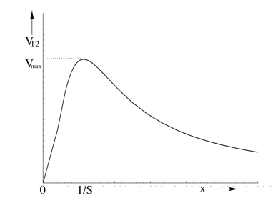
Figure 2: The string self-interaction potential as a function of relative separation $x$ along the string, for $p=4,5$.

This potential governs the dynamics of the Matrix string near a black hole or black brane transition, as it is approached from the weak coupling side. A bump in the potential occurs at the thermal wavelength $N/S$ for $p=4,5$ (five or four noncompact spatial directions); in these dimensions, the correspondence transition to a black hole is indeed caused by the string’s self-interaction, as discussed in [13]. For smaller $p$ (more noncompact spatial directions), there is no bump; similarly, in [13] the self-interactions could not cause a spontaneous collapse to a black object. We will see that the height of the bump is proportional to the gravitational coupling, such that it ‘confines’ excitations of the string on the strong-coupling side of the correspondence transition.

This result supports a suggestion [14, 15] to describe the black hole phase as clustered Matrix SYM excitations of size $N/S$. These correlated clusters were invoked in order that the object with $N>S$ can be localized in the longitudinal direction. Such a localization necessarily involves the longitudinal momentum physics of Matrix theory. We find that a plausible argument for the dynamics with this potential gives the previously identified correspondence curves as the boundaries of validity of the matrix string phase. For $N<S$, one finds the transition to the interacting $p+1$ SYM phase shown in Figure (1); while for $N>S$, one finds the transition to the matrix black hole phase. Accounting for the latter transition requires taking into consideration longitudinal momentum transfer effects as in [14]; we justify this by a string theory amplitude calculation involving winding number exchange in a dual picture. We thus conclude that we have identified the characteristics of the microscopic mechanism of black hole formation from the SYM point of view.

The plan of the presentation is as follows: in section 2, we review the two conjectures (Matrix and Maldacena) we will use in the analysis of the phase diagram. In section 3, we bring together previous observations with some new ones to map out the phase diagram for the DLCQ Matrix string. Section 4 extends our arguments at the triple point to the cases of singly and doubly charged black holes. We also discuss a toy mechanism for clustering of SYM excitations for the singly charged case, at the BFKS point. Section 5 discusses the self-interaction of the Matrix string, the identification of the bump potential and comments about its dynamics. We outline in the Appendices the calculation of the potential, and a scattering amplitude calculation relevant the issue of longitudinal momentum transfer physics.

As we were finalizing the manuscript, a paper discussing related issues [16] came to our attention.

2 A couple of conjectures

2.1 The Matrix conjecture

A convenient way to summarize the Matrix theory conjecture is to say that DLCQ M-theory on $T^{p}$ with $N$ units of longitudinal momentum is a particular regime of an auxiliary ‘${\overline{\rm M}}$-theory’ which freezes the dynamics onto a subsector of that theory. Consider such an ${\overline{\rm M}}$-theory, with eleven-dimensional Planck scale ${\bar{\ell}}_{{\rm pl}}$ (which we denote (${\overline{\rm M}}$,${\bar{\ell}}_{{\rm pl}}$)) on a $p+1$d dimensional torus of radii ${\bar{R}}_{i}$, $i=1\ldots p$, and $\bar{R}$ the ‘M-theory circle’ of reduction to type $\overline{\rm IIA}$ string theory, in the limiting regime

$${\bar{\ell}}_{{\rm pl}}\rightarrow 0,\ \ \ \mbox{with }x\equiv{{\bar{\ell}}_{{\rm pl}}^{2}\over\bar{R}}\ \ \ \mbox{and }y_{i}\equiv{{\bar{\ell}}_{{\rm pl}}\over\bar{R}_{i}}\ \ \ \mbox{fixed},$$ (3)

and $N$ units of KK momentum along $\bar{R}$. It is proposed that [7, 17]

• This theory is equivalent to an ($M$,$\ell_{{\rm pl}}$) theory on the DLCQ background we denote by $D^{1,1}\times T^{p}\times{\bf R}^{9-p}$, where $D^{1,1}$ is a $1+1$ dimensional subspace compactified on a lightlike circle of radius $R_{+}$, and the torus $T^{p}$ has radii $R_{i}$ ($i=1\ldots p$). The map between the two theories is given by

  $$x={\ell_{{\rm pl}}^{2}\over R_{+}},\ \ \ y_{i}={\ell_{{\rm pl}}\over R_{i}},$$ (4)

  with $N$ units of momentum along $R_{+}$.

• The dynamics of the ${\overline{\rm M}}$ theory in the above limit can be described by a subset of its degrees of freedom, that of $N$ D0 branes of the $\overline{\rm IIA}$ theory, up to a certain UV cutoff.

The two propositions above, in conjunction, are referred to as the Matrix conjecture [7, 17].

T-dualizing on the $\bar{R}_{i}$’s, we describe the D0 brane physics by the $p+1$d SYM of N D$p$ branes wrapped on the dualized torus. We remind the reader of the dictionary needed in this process

$$\bar{R}= ~{}\bar{g}_{s}^{\prime}{\bar{\ell}}_{{{s}}}\ \ \ {\bar{\ell}}_{{\rm pl}}^{3}=\bar{g}_{s}^{\prime}{\bar{\ell}}_{{{s}}}^{3}\ ,$$

$$\bar{g}_{s}= ~{}\bar{g}_{s}^{\prime}{{\bar{\ell}}_{{{s}}}^{p}\over\Pi\bar{R}_{i}}\ \ \ \Sigma_{i}={{\bar{\ell}}_{{{s}}}^{2}\over\bar{R}_{i}}\ .$$ (5)

The first line is the ${\overline{\rm M}}-\overline{\rm IIA}$ relation, the second that of T-duality. The limit (3) then translates in the new variables to

$$\bar{\alpha}^{\prime}\rightarrow 0\quad,\quad\quad\mbox{with }\ \ g_{Y}^{2}=(2\pi)^{p-2}\bar{g}_{s}{{\bar{\alpha}}}^{\prime(p-3)/2}\ \ \ \mbox{and }\Sigma_{i}\ \ \ \mbox{fixed}\ ,$$ (6)

where the nomenclature $g_{Y}^{2}$ and $\Sigma_{i}$ refers to the coupling and radii of the corresponding $p+1$d $U(N)$ SYM theory, whenever it is well defined in this limit, i.e. for $p\leq 3$.

For $p>3$, we see from (6) that $\bar{g}_{s}\rightarrow\infty$, the dilaton at infinity diverges (i.e. in the UV of the field theory, according to Maldacena’s conjecture [8]); this is a statement of the non-renormalizability of the corresponding SYM: New physics sets in the UV. For $p=4$, the D-branes physics is the IR limit of the six-dimensional (2,0) theory; while for $p=5$, it is that of a weakly coupled IIB NS5 brane [18, 19]. We ignore hereafter all cases with $p>5$. In summary, only at low enough energies the 4+1d and 5+1d SYM yield a proper coarse-grained description of the needed dynamics.

2.2 The Maldacena conjecture

It is proposed [8] that in the limit (6), one can identify the physics of the SYM QFT at different energy scales with the supergravity solution that is cast by the branes, whenever such a solution is well defined. One is to identify string theory excitations of the supergravity background with those of the QFT; this is essentially a correspondence between closed and open string dynamics.

Here, we will study finite temperature physics. We will therefore make use of the thermodynamic version of the above statement, which identifies the finite temperature vacuum of the SYM describing $N$ D$p$ branes with the geometry of the horizon region of the near extremal supergravity solution the branes cast about them, whenever such a solution is sensible [9]. In particular, we can extract the thermodynamics of SYM at finite temperature in its non-perturbative regimes. Correlation functions in the SYM probe different distances from the horizon in the supergravity solution as one changes the separation of operator insertions relative to the SYM correlation length (thermal wavelength); coarse graining the SYM theory to lower energies corresponds to moving towards to the center of the supergravity solution, up until the near extremal horizon [20].

Our strategy will be to use the Maldacena conjecture as a tool, to study the thermodynamics of Matrix strings and black holes; and conversely, to learn about the phase diagram of supersymmetric Yang-Mills theory on the torus.

3 A thermodynamic road-map

3.1 Preliminaries

A DLCQ IIA theory descends from the DLCQ $M$ theory described above; we choose string scale compactification

$$R_{i}\sim\ell_{{{s}}}\ \ \ \mbox{for }i=1\ldots p-1\ ,$$ (7)

with

$$R_{p}=g_{s}\ell_{{{s}}}\ \ \ \ell_{{\rm pl}}^{3}=g_{s}\ell_{{{s}}}^{3}\ ,$$ (8)

and a perturbative IIA regime

$$g_{s}<1\ .$$ (9)

We can in principle relax (7) at the expense of introducing new state variables, and a more complicated (and richer) phase diagram; for simplicity, we will stick to this ‘IIA regime’. Using the equations in the previous section, we can write the dictionary between our IIA theory and the Matrix SYM

$$g_{Y}^{2} = ~{}(2\pi)^{p-2}(ag_{s})^{p-3}\ ,$$

$$\Sigma_{i} = ~{}g_{s}a\ \ \ \mbox{for }i=1\ldots p-1\ ,$$

$$\Sigma_{p} = ~{}a\ ,$$ (10)

$$V \equiv ~{}\Sigma_{i}^{p-1}\Sigma_{p}=g_{s}^{p-1}a^{p}\ ,$$

with

$$a\equiv{\alpha^{\prime}\over R_{+}}\ .$$ (11)

We chose (9) so that we have $\Sigma_{i}<\Sigma_{p}$, simplifying our analysis later.

We study finite temperature physics of this IIA theory with the finite temperature vacuum of the corresponding SYM. As mentioned in the introduction, we confine our analysis to $p=4$ and $p=5$.

3.2 Validity of SYM

Given that we are working with Matrix theory on $T^{4}$ and $T^{5}$, the first question that must be addressed concerns the validity of the description, given that SYM 4+1d and 5+1d are non-renormalizable. New degrees of freedom are required to make sense of the SYM dynamics as we probe it in the UV, i.e. as we navigate outward in the corresponding supergravity solution. These new degrees of freedom for SYM 4+1d and 5+1d are associated with the onset of strong coupling dynamics; the validity of the theories at different energy scales is then determined by looking at the size of the dilaton vev at different locations in the supergravity solution. For finite temperatures, physics at the thermal wavelength of the SYM is identified with physics at the horizon of the near extremal solution [9, 21]

$$ds^{2}_{\rm hor}=\alpha^{\prime}\left({U^{(7-p)/2}\over g_{Y}\sqrt{d_{p}N}}d\sigma_{i}^{2}+g_{Y}\sqrt{d_{p}N}U^{(p-3)/2}d\Omega_{8-p}^{2}\right)\ .$$ (12)

We are looking at a fixed time and radial slice; the radial variable is $U$, the $\sigma_{i}$’s are coordinates along the brane with identification $\sigma_{i}\sim\sigma_{i}+\Sigma_{i}$; $d_{p}$ is a numerical coefficient; and $U_{o}$ is the location of the horizon, related to the SYM entropy [9]

$$U_{o}^{p-9}\sim(g_{Y}^{2})^{-3}S^{-2}NV^{2}\ .$$ (13)

The dilaton vev is

$$e^{\phi}=(2\pi)^{2-p}g_{Y}^{2}\left({g_{Y}^{2}d_{p}N\over U^{7-p}}\right)^{(3-p)/4}\ .$$ (14)

The finite temperature vacuum of the 4+1d and 5+1d SYM is a valid thermodynamic description of the DLCQ IIA theory (by the two conjectures stated earlier) when

$$\left.e^{\phi}\right|_{U_{o}}\ll 1\Rightarrow S\ll N^{{8-p\over 7-p}}g_{s}^{-1}\ .$$ (15)

Note that this is a purely geometric statement, in terms of the horizon area and string coupling; it will be seen to be insensitive to finite size effects due to the transverse torus. We then choose to work on a two dimensional cross section in the $S$-$g_{s}$ plane of the thermodynamic phase diagram, with fixed $N\gg 1$. In principle, one is to take the thermodynamic limit $N\rightarrow\infty$ with $N/S$ fixed, to see criticality; transition between phases at finite $N$ discussed here are smooth crossovers. It is expected that, in the infinite $N$ limit, the physics tends to the appropriate critical behavior.

Let us for a while ignore the effects of the transverse torus. In the regime where the curvature of the supergravity solution at the horizon is less than the string scale,

$$S\gg N^{{p-6\over p-3}}g_{s}^{-1}\ ,$$ (16)

the SYM statistical mechanics obeys the equation of state [9, 21, 22]

$$E_{int}^{p-9}\sim S^{2(p-7)}(g_{Y}^{2})^{p-3}N^{7-p}V^{5-p}\ .$$ (17)

Beyond this regime, we have weakly coupled SYM, roughly a free gas of $N^{2}$ gluons. These statements are graphically summarized in Figure 3.

Figure 3: The entropy $S$ versus $g_{s}$ phase diagram showing the region of validity of the SYM description, and the boundary between the free and interacting phases, ignoring finite size effects. We assume $N,S\gg 1$, and $g_{s}<1$, and fix $N$ for a given diagram.

Our assumption that finite size effects, due to the compactification of the $\sigma_{i}$ variables, are of no relevance is the statement that, for high enough temperature (i.e. for thermal wavelengths short enough with respect to the effective sizes of the torus), the local thermodynamics is similar to that of the uncompactified case. The rest of this section is the study of the breakdown of this regime; we would like to paint over Figure 3 new phases arising due to the compactification of the background. In particular, we will argue that the geometry describing the interacting $p+1$d SYM phase gets modified due to the two transition mechanisms outlined in the Introduction; consequently, the correspondence line of equation (16) is changed.

3.3 Finite size effects

A finite size effect in the supergravity regime that was determined in the work of [2, 3, 4, 5] is the effect of the DLCQ radius $R_{+}$ on the geometry. We saw from equation (2) that a black hole is localized longitudinally when $N>S$. The black hole equation of state is

$$E^{p-9}_{bh}\sim E_{int}^{p-9}\left({N\over S}\right)^{2}\ .$$ (18)

The process of minimizing the Gibbs energies between the black hole and interacting SYM phases yields a black hole phase as in Figure 4, independent of $p$, which is the BFKS observation [2, 3, 4];

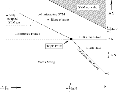
Figure 4: For the convenience of the reader, we reproduce Figure (1): The proposed thermodynamic phase diagram for the $p+1$d SYM on the torus, i.e. the DLCQ IIA theory.

but we now see that the Maldacena conjecture justifies the procedure.

The Schwarzschild black hole geometry will become stringy when its curvature near the horizon becomes of the order of the string scale; the emerging state is a Matrix string in the Matrix conjecture language, i.e. a $1+1$ state with $Z_{N}$ holonomy on $\Sigma_{p}$. Minimizing the Gibbs energy between the Matrix string and Matrix black hole phases leads to the Horowitz-Polchinski correspondence curve [1, 13]

$$S\sim g_{s}^{-2}\ .$$ (19)

This is a statement independent of $N$ and $p$. At $g_{c}\sim N^{-1/2}\sim N_{\rm\scriptscriptstyle osc}^{-1/4}$, where $N_{\rm\scriptscriptstyle osc}$ is the string oscillator level, there exists an interesting critical point.

We next deal with finite size effects in the interacting $p+1$d SYM phase which are due to the other radii $\Sigma_{i}$. This is problematic since, unlike the free case, the strongly coupled SYM may acquire at finite temperature a nontrivial vacuum; for example, a vacuum characterized by a holonomy sewing branes together. It is in such a regime that Susskind observed for the case $p=3$ that the effective size of the SYM box is bigger than $\Sigma_{i}$ [6]. In the spirit of Susskind’s transition, and inspired by the existence of a Matrix string phase on the left of the phase diagram, we suggest that the finite size effect can be probed by comparing the Gibbs energies of the interacting $1+1$d and $p+1$d phases. Using equation (17), we get a critical line at

$$S\sim\sqrt{N}g_{s}^{-1}\ ,$$ (20)

independent of $p$ and matching onto the ‘triple point’ of correspondence. Even so, for these values of $S$, $N$ and $g_{s}$, the $1+1$d SYM is not described by the supergravity solution whose equation of state we used. The analogue of Figure 3 with $p=1$ has the correspondence curve on the strong coupling side of the line where $e^{\phi}=1$; in other words, the D string supergravity solution is strongly coupled, as noted in [9]. However, the S-dual is the weakly coupled supergravity solution of a fundamental IIB string source; its equation of state is the same as the one used above, given that the entropy is to be calculated in the Einstein frame. The curvature at the horizon of the S-dual solution becomes of order the string scale at precisely (20) [9], beyond which a Matrix string description emerges. We can further check the correctness of this conclusion by matching the $p+1$d interacting SYM gas equation of state with that of the Matrix string, the latter being the dominant phase on the other side of this correspondence curve. The result is again (20). We conclude that the $p+1$d interacting SYM makes a transition to a Matrix String at (20). This is shown in Figure 4.

From the supergravity side, we note that, both the $p+1$d SYM $\rightarrow$ $1+1$d SYM transition and the Matrix black hole $\rightarrow$ Matrix string transition are correspondence regimes where the geometry, that of a near extremal fundamental string and that of a black hole respectively, has curvature at the horizon of order of the string scale [1]. On the other hand, the BFKS transition is that of longitudinal localization of the supergravity solution [5].

We can now understand the observation of Susskind from the phase diagram of Figure 4. From the interacting $p+1$d SYM side, one can consider the effective box sizes (i.e. the critical thermal wavelengths) as one approaches the various transitions. The effective box size is defined by $T_{c}\Sigma_{\rm eff}\sim 1$, where as usual the temperature is determined from $T\sim E/S$. This yields for the $N\sim S$ transition

$$\Sigma_{\rm eff}\sim\Sigma_{p}\left(Ng_{s}^{2}\right)^{2/(9-p)}\ ,$$ (21)

and for the Matrix String/$p+1$d SYM transition

$$\Sigma_{\rm eff}\sim\Sigma_{i}\sqrt{N}=\Sigma_{p}g_{s}\sqrt{N}\ .$$ (22)

The bound of Susskind (equation (3.5) of [6]) is simply that, starting with the $p+1$d SYM phase at high temperature, one sees a transition to the Matrix black hole phase as the temperature is lowered only if (in the IIA variables)

$$g_{s}>N^{-1/2}\ .$$ (23)

This is clear from Figure 4.

Finally, we note that we assumed above that there exists a well defined matrix string description for $N<S$. In this regime, the thermal wavelength on the Matrix string is smaller than the UV cutoff imposed by the discretized nature of the matrices. Our procedure may be equivalent to an analytical continuation of the matrix string phase into a regime where the description may not be fully justified; this is in the same spirit as the extension of the Van der Waals equation of state into the gas-liquid coexistence region, which one uses to identify the emergence of the liquid phase[23]. For small enough coupling $g_{s}$, we expect the Matrix string to evaporate into a perturbative SYM gas, as shown on Figure 4. Furthermore, the regime $N<S$ is similar to the Hagedorn regime [24, 25], in that the temperature remains constant as the system absorbs heat. We speculate that the $N<S$ regime of the Matrix string near the triple point is characterized by a coexistent phase of a string with SYM vapor. We defer a detailed analysis of this issue to future work.

As a unifying probe for all the transitions, we observe that the ‘mass per unit charge’ $q$ defined in (1) scales on the various transition curves as

Matrix String-$p+1$d SYM Transition	$\rightarrow$	$q^{-1}\sim g_{\rm eff}\ell_{{{s}}}$
Matrix String-Coexistence Phase Transition	$\rightarrow$	$q^{-1}\sim\ell_{{{s}}}$
Matrix String-Black Hole Transition	$\rightarrow$	$q^{-1}\sim g_{\rm eff}^{2}\ell_{{{s}}}$
Black Hole-$p+1$d SYM Transition	$\rightarrow$	$q^{-1}\sim g_{\rm eff}^{2/(9-p)}\ell_{{{s}}}$

with the effective coupling

$$g_{\rm eff}^{2}\equiv g_{s}^{2}N\ .$$ (24)

From the point of view of the DLCQ string theory characterized by the parameters $g_{s}$, $\ell_{{{s}}}$ and $N$, this scaling on the transition curves is a non-trivial signature of a unifying framework underlying the physics of criticality of the theory. Note also that the $g_{s}^{2}N$ combination is not the ’t Hooft coupling of the Matrix SYM description, equation (10); recall that $g_{s}$ is a modulus of the torus compactification.

From the point of view of field theory, the various transitions that we have identified are predictions about the thermodynamics of 4+1d, 5+1d SYM on the torus well into non-perturbative field theory regimes.

4 Comments about charged phases

In this section, we will focus on the triple point, where the correspondence and localization effects coincide, and present general considerations of relevance to singly and doubly charged black holes. We will see that, at the critical point, charged black holes are characterized by $N/S>1$. For the singly charged case, by making use of ’t Hooft holonomies on the torus, we will sketch a simple dynamical mechanism by which the system can cluster its SYM excitations at the triple point so as to account for the ratio $N/S$.

Let us begin by rephrasing part of our previous analysis in a slightly different language, using the IMF formalism. Consider a black hole in $D$ dimensions arising from M-theory on $T^{p+1}$, and define $D+p=10$. Denote the size of the M-theory circle by $R$, and suppose the other circles have the characteristic sizes $R_{i}$ as in Section 2. The horizon radius $r_{0}$ of a black hole of mass $M$ is

$$r_{0}^{D-3}={\ell_{{\rm pl}}^{9}\over RR_{1}\cdots R_{p}}M\sim\Bigl{(}{\ell_{{\rm pl}}^{3}\over R}\Bigr{)}^{(D-3)/2}$$ (25)

at the correspondence point where the horizon size is the string scale $\ell_{{{s}}}^{2}\sim\ell_{{\rm pl}}^{3}/R$. To reach the correspondence point for a given mass black hole, one tunes the string coupling $g_{s}\sim(\ell_{{\rm pl}}/R)^{3/2}$ while holding the size of the compactification torus (other than the M-theory circle) fixed in string units. Therefore let all the $R_{i}=\lambda\ell_{{{s}}}$; one finds

$$M\ell_{{{s}}}\sim\lambda^{d-1}g_{s}^{-2}\ .$$ (26)

At this point, the string entropy

$$S_{s}\sim\sqrt{N}_{\rm\scriptscriptstyle osc}$$ (27)

is of the same order of magnitude as the black hole entropy ($G_{\scriptscriptstyle D}$ is the $D$-dimensional Newton constant)

$$S_{\scriptscriptstyle BH}\sim r_{0}^{D-2}G_{\scriptscriptstyle D}^{-1}\ .$$ (28)

To work at the triple point, we demand that the string coupling is tuned so that the horizon size is of order the string scale, as dictated by the correspondence principle, and that the black hole is placed in a small box and boosted to the black hole/black string transition [2, 3, 4, 5, 26, 27], so that it can be described by matrix theory as a D-brane fluid. At the latter point, the entropy of an uncharged black hole is related to the momentum $P=N/R$ of the boosted hole by $S_{\scriptscriptstyle BH}\sim N=RP$. In terms of general relativity, the effect of the boost is to expand the proper size of the box near the black hole so that it ‘just fits inside’. For a small box and a large black hole, the system is highly boosted at the string/hole transition. In the IMF, the weak-coupling string that (according to the correspondence principle) approximates the black hole, has an energy

$$E_{\scriptscriptstyle LC}\sim\Sigma T^{2}\sim{1\over P\ell_{{{s}}}^{2}}N_{\rm\scriptscriptstyle osc}\ ,$$ (29)

where $\Sigma$ is the length of the string, $T$ is its temperature, $N_{\rm\scriptscriptstyle osc}$ is the oscillator excitation number, and $P=N/R$ is the longitudinal momentum. From this we find the temperature is given by

$$T\sim{RN_{\rm\scriptscriptstyle osc}^{1/2}\over N\ell_{{{s}}}^{2}}\ .$$ (30)

On the other hand, one expects the black hole to emit Hawking radiation at temperature

$$T_{H}\sim{e^{-\alpha}\over r_{0}}\sim{R\over r_{0}^{2}}\ ,$$ (31)

where $\alpha$ is the rapidity of the boost needed to fit the hole in the longitudinal box. The temperature of emitted quanta must be the same as the temperature of the gas on the string; equating the two expressions (30) and (31), we find

$${N_{\rm\scriptscriptstyle osc}^{1/2}\over N}\sim{\ell_{{{s}}}^{2}\over r_{0}^{2}}\ .$$ (32)

Now the boost quantum $N$ is the entropy of the black hole, as is the square root of the oscillator number; the left-hand side is of order unity, and therefore the black hole is of order the string size. This is a rephrasing of the observation (19) of Section 3, at the triple point. Moving away from this point by boosting to $N>S$ is a canonical operation; $S\sim\Sigma T$ for a string, and $\Sigma\propto N$ while $T\propto 1/N$. Note that the number of matrix partons in a thermal wavelength of the matrix string at the correspondence point is always $N_{\rm cl}\sim N/S$, in agreement with the proposal of [14].

For a singly-charged hole, the mass, charge and entropy are given by

$$M \sim ~{}G_{D}^{-1}r_{0}^{D-3}({\rm ch}^{2}\gamma+{\textstyle{1\over D-3}})$$

$$Q \sim ~{}G_{D}^{-1}r_{0}^{D-3}{\rm sh}\gamma{\rm ch}\gamma$$ (33)

$$S \sim ~{}G_{D}^{-1}r_{0}^{D-2}{\rm ch}\gamma\ \hfill$$

in terms of the ‘charge rapidity’ $\gamma$. The Hawking temperature in the boosted frame is

$$T_{H}\sim{e^{-\alpha}\over r_{0}\;{\rm ch}\,\gamma}\ ;$$ (34)

again equating this temperature with the string temperature (30) and setting the horizon size equal to the string scale correctly yields

$$S_{\scriptscriptstyle BH}\sim N_{\rm\scriptscriptstyle osc}^{1/2}\sim{N\over{\rm ch}\,\gamma}\ .$$ (35)

This implies that, for the charged case, even at the BFKS point, $N/S>1$. This ratio was interpreted in [14] as the size of clusters of partons making up the black hole phase. Therefore, the charged black hole is to be described at the BFKS point as a gas of clusters of size ${\rm ch}\gamma$.

We can see a mechanism for this dynamics with the following argument. Consider the Matrix string limit of Matrix theory on $T^{2}$. Matrix string transverse excitations are stored in the scalars of the $2+1$ SYM, on the diagonal of the matrices, with the eigenvalues sewn by boundary conditions involving the shift operator [28]. Off-diagonal constant modes describe the effect of the W bosons stretched between the strands of the string; their one-loop fluctuations give the effective gravitational interaction of the bits of the Matrix string. Given a holonomy describing a singly charged Matrix string phase, one can ask what is the interaction potential between two points on the strands, or between two matrix elements on the D-string. Fixing a winding charge $Q$, a magnetic field must be turned on

$$B_{12}={R\over N}Q\ .$$ (36)

This induces a holonomy on the 2-torus, with ’t Hooft style boundary conditions [29]. Extending these conditions onto the scalars $X^{i}$, we get

$$X^{i} = ~{}V^{k}X^{i}V^{-k}$$ (37)

$$X^{i}(\sigma+\Sigma) = ~{}U^{l}X^{i}(\sigma)U^{-l}\hfill\ ,$$

with $U_{ij}=\delta_{i,j-1}$, $V_{ij}=diag\left[{\rm exp}(2\pi i(m-1)/N)\right]$, $m=1,...,N$; and $kl=\alpha^{\prime}Q/R_{i}=\ell_{{{s}}}Q$. This configuration describes a system consisting of $l$ strings, and requires the vanishing of some of the off-diagonal elements between the matrix strands. This latter effect reduces the strength of the interaction of the strings when the off-diagonal modes are integrated, by a $Q$ and $l$ dependent factor. Modeling the system through the interaction of the zero modes, and taking into account the multiplicity factor in the interaction resulting from the boundary conditions (37), we find an energy for the gas as a function of $l$

$$E(l)\sim{N\over lR}v^{2}-Kl\left({N\over l}\right)^{2}{Q\ell_{{{s}}}\over N}{G_{D}\over R^{3}}{v^{4}\over r^{7-d}}\ ,$$ (38)

with $K$ a numerical coefficient independent of $N$ and $l$. Applying the uncertainty principle and the virial theorem [5] at the correspondence point $r_{0}\sim\ell_{{{s}}}$ then yields the scaling

$${N\over l}\sim{\rm ch}\gamma\ ,$$ (39)

in agreement with (35); i.e., it is energetically favorable for the system to settle into a phase of clusters of matrices of size $N/S\sim{\rm ch}\gamma$.

Finally, a doubly-charged hole is obtained in the correspondence principle from a string carrying both winding and momentum in compact directions. The IMF energy and the worldsheet temperatures of left- and right-movers are

$$E_{\scriptscriptstyle LC} \sim ~{}\Sigma(T_{L}^{2}+T_{R}^{2})\sim{N^{\rm\scriptscriptstyle osc}_{L}+N^{\rm\scriptscriptstyle osc}_{R}\over P\ell_{{{s}}}^{2}}$$

$$T_{L,R} \sim ~{}{RN_{L,R}^{1/2}\over N\ell_{{{s}}}^{2}}\hfill\ .$$ (40)

At the string-hole transition, one has

$$P \sim ~{}G_{\scriptscriptstyle D}^{-1}r_{0}^{D-3}({\rm ch}^{2}\gamma_{w}+{\rm ch}^{2}\gamma_{p})e^{\alpha}$$

$$S \sim ~{}G_{\scriptscriptstyle D}^{-1}r_{0}^{D-2}{\rm ch}\,\gamma_{w}~{}{\rm ch}\,\gamma_{p}\hfill\ ,$$ (41)

from which one finds the relation

$$N\sim S\;{{\rm ch}^{2}\gamma_{w}+{\rm ch}^{2}\gamma_{p}\over{\rm ch}\,\gamma_{w}~{}{\rm ch}\,\gamma_{p}}$$ (42)

between the longitudinal boost quantum and the entropy. Note that $S\sim N_{{\rm\scriptscriptstyle osc},L}^{1/2}+N_{{\rm\scriptscriptstyle osc},R}^{1/2}\propto{\rm ch}\gamma_{w}{\rm ch}\gamma_{p}$, while the Hawking temperature must be $T_{H}={2T_{L}T_{R}\over T_{L}+T_{R}}\propto({\rm ch}\gamma_{w}{\rm ch}\gamma_{p})^{-1}$. A consistent assignment of worldsheet oscillator numbers with respect to these quantities is

$$N_{L,R}\sim\left(G_{D}^{-1}r_{0}^{D-2}{\rm ch}(\gamma_{w}\pm\gamma_{p})\right)^{2}\ ,$$ (43)

so that the oscillator entropy agrees with the black hole entropy (41), and the Hawking temperature determined from (40) is of the right order . We note that we have again $N/S>1$ at the triple point due to the presence of KK charges.

Thus, in general it is necessary that the matrix black hole consist of coherent clusters of matrix partons even at the BFKS transition; and that, at the correspondence point, the number of partons in a cluster is the same as the number of strands of the matrix string lying within a thermal wavelength. Both of these facts support the analysis of [14].

5 The interacting Matrix string

In this section, we come back to the neutral case, away from the triple point, attempting to probe the dynamics in greater detail from the Matrix String side. In [14], it was argued that the Matrix black hole phase, as a SYM field configuration, can be thought of as a gas of $S$ clusters of D0 branes, the zero modes of the SYM, each cluster consisting of $N/S$ partons. The system is self-interacting through the $v^{4}/r^{7}$ interaction, or its smeared form on the torus.

This phase of clustered D0 branes may be an effective description, i.e. thermodynamically strongly correlated regions of a metastable state; or more optimistically, it might be a microscopic description associated with formation of bound states like in BCS theory. We will try here to investigate the Matrix string dynamics so as to reveal the signature of the clusters as we approach the correspondence curve. The aim is to identify a possible dynamical mechanism for black hole formation, and determine the correspondence curve from such a microscopic consideration.

In Section 5.1, we derive the potential between two points on the Matrix string; in view of the Matrix conjecture, we can do this by expanding the DBI action of a D-string in the background of a D-string. We then evaluate the expectation value of this potential in the free string ensemble at fixed temperature. In Section 5.2, we analyze the characteristic features of the potential, particularly noting the bump for $p=4,5$ that we alluded to in the Introduction. In Section 5.3, we comment on the dynamics implied by the potential, particularly in regard to the phase diagram derived earlier.

5.1 The potential

In this section, we derive the potential between two points on the Matrix string by expanding the DBI action for a D-string probe in the background geometry of a D-string. We then check the validity of the DBI expansion, and evaluate the expectation value of the potential in the thermal ensemble of highly excited Matrix strings. The details of the finite temperature field theory calculations are collected in Appendix A.

A IIA string in Matrix string theory is constructed in a sector of field configurations described by diagonal matrices, with a holonomy in $Z_{N}$; a nonlocal gauge transformation converts this into ’t Hooft-like twisted boundary conditions on the transverse excitations of the eigenvalues of the matrices, as described in detail in [28, 30, 31, 32]. The conclusion is that the eigenvalues are sewn together into a long string, and a IIA string emerges as an object looking much like a coil or ‘slinky’ wrapped on $\Sigma_{p}$. The self-interactions of this string are described by integrating out off-diagonal modes between the well-separated strands. Alternatively, making use of the Matrix conjecture, this effective action can be obtained from supergavity, by expanding the Born-Infeld action of a D-string in the background of a D-string. We will follow this prescription to calculate the gravitational self-interaction potential between two points on a highly excited Matrix string.

The Born-Infeld action for N D-strings is given by [33]

$$S=-{1\over 2\bar{\alpha}^{\prime}\bar{g}_{s}}\left[\int d^{2}\sigma e^{-\phi}\mbox{Tr}\mbox{Det}^{1/2}\left(G_{ab}+B_{ab}+2\pi\alpha^{\prime}F_{ab}\right)-N\int C_{RR}^{(2)}\right],$$ (44)

where we have assumed commuting matrices so that there is no ambiguity in matrix orderings in the expansion, and $\bar{g}_{s}$ is the dilaton vev at infinity. We choose $\sigma^{1}$ to have radius $\Sigma_{p}$, turn off gauge and NS-NS fluxes,

$$B_{ab}=F_{ab}=0\ ,$$ (45)

and choose the static gauge

$$X^{0} = ~{}\sigma^{0}\mbox{1}\ ,$$ (46)

$$X^{1} = ~{}\sigma^{1}\mbox{1}\ .$$

A single D-string background in the string frame is given by [34]

$$ds_{10}^{2} = ~{}h^{-1/2}(-dt^{2}+dx^{2})+h^{1/2}(d\vec{x})^{2}$$

$$\vskip 6.0pt plus 2.0pt minus 2.0pte^{\phi} = ~{}h^{1/2}\hfill$$ (47)

$$C_{01} = ~{}h^{-1}\hfill$$

$$h = ~{}\left({r_{0}\over r}\right)^{7-p}\ ,$$

(recall $p$ is the torus dimension) and we define $D\equiv 7-p$. The string is taken to have no polarizations on the torus, nor any KK charges. Here, we have followed the prescription in [35, 36], where we T-dualized the D-string solution to a D0 brane, lifted to 11 dimensions, compactified on a lightlike direction, and T-dualized the solution to the one above. The only change is in replacing $1+(r_{0}/r)^{7-p}\rightarrow(r_{0}/r)^{7-p}$. By Gauss’ law,

$$r_{0}^{D} = ~{}c_{D}{g_{s}^{2}\over R_{+}^{2}}\ell_{{{s}}}^{9-p}\ ,$$ (48)

$$c_{D} \equiv ~{}{(2\pi)^{7}\over 2\pi^{D/2}}\Gamma(D/2)\ ,$$

where we have made use of the needed dualities to express things in our IIA description. Putting in the background, we have

$$S = ~{}-{1\over\alpha^{\prime}}\int^{\Sigma_{p}N}\ h^{-1}\left(1+hK+h^{2}V\right)^{1/2}-h^{-1}$$ (49)

$$K \equiv ~{}{X^{\prime}}^{2}-{\dot{X}}^{2}=4\partial_{+}X.\partial_{-}X$$

$$\vskip 6.0pt plus 2.0pt minus 2.0ptV \equiv ~{}4((\partial_{+}X.\partial_{-}X)^{2}-(\partial_{+}X)^{2}(\partial_{-}X)^{2})\ .$$

We note that, as the limit of the action indicates, we have made use of the $Z_{N}$ holonomy that sews the rings of the slinky together. Expanding the square root yields the Hamiltonian

$$H=\int^{\Sigma_{p}N}{1\over 2\alpha^{\prime}}({\dot{X}}^{2}+{X^{\prime}}^{2})+c_{D}^{\prime}{g_{s}^{2}\ell_{{{s}}}^{7-p}\over R_{+}^{2}r^{7-p}}\left\{(\partial_{+}X)^{2}(\partial_{-}X)^{2}-\left[(\partial_{+}X)^{2}+(\partial_{-}X)^{2}\right](\partial_{+}X.\partial_{-}X)\right\}\ .$$ (50)

Let us check the validity of the DBI expansion we have performed. We would like to study dynamics of the string squeezed at most up to the string scale, the correspondence point; setting $r\sim\ell_{{{s}}}$ in $h$, we get

$$h\sim\left({g_{s}\ell_{{{s}}}\over R_{+}}\right)^{2}\ .$$ (51)

From elementary string dynamics (equations (27),(29)), we have

$$\left\langle K\right\rangle\sim\left({R_{+}S\over\ell_{{{s}}}N}\right)^{2}\ ,$$ (52)

where brackets indicate thermal averaging at fixed entropy $S$. It can be shown from the results of the next section that

$$\left\langle V\right\rangle_{max}\sim\left\langle K\right\rangle^{2}\ ,$$ (53)

and that $\left\langle V\right\rangle$ will have a definite maximum for all $p$. We now see from (49),(51),(52), and (53), that our DBI expansion is a perturbative expansion in

$$\varepsilon=g_{s}{S\over N}\ .$$ (54)

We then need

$$S\ll Ng_{s}^{-1}\ .$$ (55)

A glance at Figure 4 reveals that we are well within the region of interest.

The potential in this expression is the interaction energy between a D-string probe and a D-string source. Using the residual Galilean symmetry in the DLCQ, and assuming string thermal wavelengths $>\Sigma_{p}$ (the ‘slinky regime’), we deduce that the potential between two points on the Matrix strings denoted by the labels $1$ and $2$ is

$$V_{12}={K}_{D}{g_{s}^{2}\ell_{{{s}}}^{5-p}\over R_{+}}{\left\{(\partial_{+}X_{r})^{2}(\partial_{-}X_{r})^{2}-\left[(\partial_{+}X_{r})^{2}+(\partial_{-}X_{r})^{2}\right](\partial_{+}X_{r}.\partial_{-}X_{r})\right\}\over\left(X_{r}^{2}\right)^{D/2}}\ ,$$ (56)

where

$$X_{r}\equiv X_{2}-X_{1}.$$ (57)

and $K_{D}$ is a horrific numerical coefficient we are not interested in.

Ideally, one should self-consistently determine the shape distribution of the string in the presence of this self-interaction; however, this is rather too complicated to actually carry out. To first order in small $g_{s}$, the effect of the potential is to weigh different regions of the energy shell in phase space [37] by a factor derived from its expectation value in the free string ensemble. We will discuss the dynamics in the presence of the potential in somewhat more detail below. For now, in light of this weak-coupling approximation scheme, we would like to calculate the expectation value of the potential in a thermodynamic ensemble consisting of a highly excited free string with fixed entropy $S$. From the Matrix string theory point of view, this is essentially a problem in finite temperature field theory, where we will deal with a two dimensional Bose gas (ignoring supersymmetry; the fermion contribution is similar) on a torus with sides $\Sigma_{p}N$ and $\beta=1/T$, $\beta$ being the period of the Euclidean time. Using Wick contractions, we can then express the potential in terms of the free Green’s functions; we defer the details to Appendix A. We get

$$V_{12}=\alpha_{D}g_{s}^{2}{\ell_{{{s}}}^{5-p}\over R_{+}}{K^{zz}_{12}K^{\bar{z}\bar{z}}_{12}\over\left(-K_{12}\right)^{D/2}},$$ (58)

where $\alpha_{D}$ is a dimension dependent numerical coefficient,

$$K_{12}\equiv K_{\Delta}\equiv-\alpha^{\prime}\left<X_{1}X_{2}\right>\equiv-\alpha^{\prime}G_{12}\ ,$$ (59)

is the Green’s function of the two dimensional Laplacian on the torus, and $K^{zz}_{12}$ is its double derivative with respect to the $z$ complex coordinate of the Riemann surface representing the Euclideanized world-sheet. We refer the reader to Appendix A for the derivation of this equation.

5.2 The thermal free string

The thermodynamic properties of the matrix string at inverse temperature $\beta$ are determined by the Green’s function of the Laplacian on the worldsheet torus of sides $(\Sigma,\beta)$, where $\Sigma\equiv\Sigma_{p}N$. It is known from CFT on the torus that this is given by[38, 39]

$$G_{12}=-{1\over 2\pi}\ln\left|{\theta_{1}\left({z\over\Sigma}|\tau\right)\over\theta^{\prime}_{1}\left(0|\tau\right)}\right|+{1\over 2\tau_{2}}\left(\mbox{Im}{z\over\Sigma}\right)^{2},$$ (60)

where

$$\tau\equiv i{\beta\over\Sigma}\equiv i\tau_{2}={i\over S}.$$ (61)

Here $\beta$ can be obtained from the free string thermodynamics of equation (30). All correlators and their derivatives must eventually be evaluated on a time slice corresponding to the real axis in the $z$ plane.

Divergences will be seen in correlators due to infinite zero point energies. The conventional approach is to introduce a normal ordering scheme giving the vacuum zero expectation value in such situations, i.e. throwing away disconnected vacuum bubbles. In our case, the string has a classical background due to its thermal excitation. To renormalize finite $T$ correlators, we subtract the zero temperature limit from each propagator. This corresponds to

$$\mbox{$\langle{f(X)}\rangle$}\sim f({\textstyle{\delta\over\delta J}})\ln Z_{T}[J]\rightarrow f({\textstyle{\delta\over\delta J}})\ln Z_{T}[J]-f({\textstyle{\delta\over\delta J}})\ln Z_{T=0}[J]=f({\textstyle{\delta\over\delta J}})\ln\Bigl{(}{Z_{T}[J]\over Z_{T=0}[J]}\Bigr{)}.$$ (62)

From the expression for $Z[J]$, we see that this amounts to correcting the Green’s functions as

$$K\rightarrow K_{T}-K_{T=0}.$$ (63)

This subtraction removes the divergent zero-point fluctuations of nearby points on the string, while leaving the effects due to thermal fluctuations.

Defining

$$x\equiv{z\over\Sigma}\ ,$$ (64)

we then have, subtracting the zero temperature part,

$$K_{\Delta}\rightarrow\alpha^{\prime}\left({1\over 4\pi}\ln g\bar{g}+{1\over 8\tau_{2}}\left(x-\bar{x}\right)^{2}\right),$$ (65)

with

$$\ln g=\sum_{n=1}\ln\left({1-2q^{n}\cos(2\pi x)+q^{2n}\over\left(1-q^{n}\right)^{2}}\right).$$ (66)

We can now make use of $\tau_{2}\ll 1$ for $S\gg 1$, to write this sum as an integral

$$\ln g={1\over 2\pi\tau_{2}}\int_{0}^{e^{-2\pi\tau_{2}}}{dv\over v}\ \ \ln\left({1-2v\cos(2\pi x)+v^{2}\over\left(1-v\right)^{2}}\right).$$ (67)

This integral can be evaluated to yield

$$\ln g={1\over 2\pi\tau_{2}}\left(2Li_{2}e^{-2\pi\tau_{2}}-Li_{2}e^{-2\pi\tau_{2}+2\pi xi}-Li_{2}e^{-2\pi\tau_{2}-2\pi xi}\right),$$ (68)

where $Li_{2}$ is the PolyLog function of base 2, related to the Lerch $\Phi$ function [40]. We then have

$$K_{\Delta}={\alpha^{\prime}\over 2\pi}\ln g\ ,$$ (69)

with $x$ here being real, and representing the equal-time separation between two points on the string, $x=x_{1}-x_{2}$, as a fraction of the total length $\Sigma$ ($0<x<1$). The asymptotics are

$$K_{\Delta}\simeq\left[\begin{array}[]{cl}\alpha^{\prime}Sx&\mbox{ for }\tau_{2}\ll 1\\ {\alpha^{\prime}\over\pi}S^{2}x^{2}&\mbox{ for }2\pi x\ll 1\end{array}\right.,$$ (70)

The first line is a well-known result of Mitchell and Turok [41] calculated originally using the microcanonical ensemble. It shows random walk scaling $\sqrt{\mbox{$\langle{R^{2}}\rangle$}}\sim N_{\rm\scriptscriptstyle osc}^{1/4}x^{1/2}$. The second line is new and valid for small separations on the string; it is the statement that within the thermal wavelength $\beta$ of the the excited string, the string is stretched, scaling as $\sqrt{\mbox{$\langle{R^{2}}\rangle$}}\sim N_{\rm\scriptscriptstyle osc}^{1/2}x$. This is intuitively expected, as regions on the string within the typical thermal wavelength will be strongly correlated in the thermodynamic sense. This change in the scaling is crucial to what we will soon see in the behavior of the potential between strands. $-K_{\Delta}$ is plotted in Figure 5.

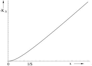
Figure 5: $-K_{\Delta}$ as a function of the string separation parameter $x$; we see the change of scaling from $x^{2}$ to $x$.

Next, consider the derivatives of the correlators, evaluated on the real axis. We have

$$\partial_{x}K_{\Delta}=\partial_{\bar{x}}K_{\Delta}={-i\alpha^{\prime}\over 2(2\pi)^{2}\tau_{2}}\ln\left({1-e^{-2\pi\tau_{2}-2\pi ix}\over 1-e^{-2\pi\tau_{2}+2\pi ix}}\right).$$ (71)

We also have

$$\partial_{x}\partial_{\bar{x}}K_{\Delta}={-\alpha^{\prime}\over 4\tau_{2}},$$ (72)

or

$$K^{z\bar{z}}_{\Delta}\rightarrow 0,$$ (73)

since we subtract the zero temperature result. The most relevant term is

$$\partial_{x}^{2}K_{\Delta}=\partial_{\bar{x}}^{2}K_{\Delta}=-{\alpha^{\prime}\over\tau_{2}}{1-e^{2\pi\tau_{2}}\cos(2\pi x)\over e^{4\pi\tau_{2}}-2e^{2\pi\tau_{2}}\cos(2\pi x)+1}+{\alpha^{\prime}\over 4\tau_{2}},$$ (74)

or

$$\Sigma^{2}K^{zz}_{\Delta}=\Sigma^{2}K^{\bar{z}\bar{z}}_{\Delta}\rightarrow-{\alpha^{\prime}\over\tau_{2}}{1-e^{2\pi\tau_{2}}\cos(2\pi x)\over e^{4\pi\tau_{2}}-2e^{2\pi\tau_{2}}\cos(2\pi x)+1}-{\alpha^{\prime}\over\tau_{2}}{1\over e^{2\pi\tau_{2}}-1}$$ (75)

(again we subtract the zero temperature part).

This yields the asymptotics

$$(N\Sigma_{p})^{2}K^{zz}_{\Delta}\simeq\left[\begin{array}[]{cl}\alpha^{\prime}S^{2}+{\pi\over 12}(5+\cos(2\pi x))(\csc(\pi x))^{2}+O(\tau_{2}^{2})\rightarrow\alpha^{\prime}S^{2}&\mbox{ for }\tau_{2}\ll 1\\ \alpha^{\prime}S^{4}x^{2}&\mbox{ for }2\pi x\ll 1\end{array}\right..$$ (76)

$K^{zz}_{\Delta}$ is plotted in Figure 6 as a function of $x$.

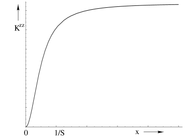
Figure 6: $K^{zz}_{\Delta}$ as a function of the string separation parameter $x$; we see the flattening of the correlation at large $x$. For small $x$, small relative stretching or motion is implied; for larger $x$, the flattening indicates a constant correlation in the relative stretching of the string.

5.3 The bump potential

We now put together equations (69) and (75) in the potential of (58) to get the asymptotics

$$V_{12}\simeq g_{s}^{2}{R_{+}^{3}\over{\alpha^{\prime}}^{3}N^{4}}\left[\begin{array}[]{cl}S^{(8-D)/2}x^{-D/2}&\mbox{ for }\tau_{2}\ll 1\\ S^{8-D}x^{4-D}&\mbox{ for }2\pi x\ll 1\end{array}\right..$$ (77)

For $p>3$, $V_{12}\rightarrow 0$ as $x\rightarrow 0$; at larger $x$, it decays as $x^{-D/2}$. At the thermal wavelength $x\sim 1/S$, both expressions give

$$V_{max}\simeq g_{s}^{2}{R_{+}^{3}\over{\alpha^{\prime}}^{3}N^{4}}S^{4}.$$ (78)

Note that in this expression the dimension dependence in the power of $S$ conspires to vanish. For $p=3$, $V_{12}\sim S^{4}$ for $x\rightarrow 0$, while for $p<3$, $V_{12}\rightarrow\infty$ for $x\rightarrow 0$; in both of these latter cases, the potential decays as $x^{-D/2}$ for larger $x$.

The conclusion can be summarized as follows. For $p=4$ and $p=5$, there exists a bump in the potential of height proportional to $S^{4}$ at the thermal wavelength on the string; for $p=3$, the bump smoothes to a flat configuration where the difference between the potential at the thermal wavelength separation and at $x=0$ is of order unity. Finally, for $p<3$, the bump disappears altogether and the potential blows up at the origin signaling the breakdown of the description. This potential is plotted in various cases in Figure 2 of the introduction and Figure 7.

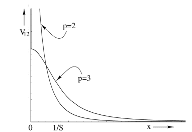
Figure 7: The potential as a function of $x$ for dimensions $p=3$ and $p=2$.

The presence or absence of the bump is a result of two competing effects: First of all, the increasingly singular short-distance behavior of the Coulomb potential (56) with increasing dimension $D$; and secondly, the strong correlation of neighboring points on the string, which makes $(\partial X_{1}-\partial X_{2})$ decrease as the separation along the string decreases (inside a thermal wavelength).

We observe that:

• The bump occurs at separations of $1/S$ of a fraction of the whole length of the string; in the matrix language, this corresponds to a bump about matrices of size $N/S$.

• The presence or absence of the bump as a function of the number of non-compact space dimensions correlates with the observations of [13], given that in the DLCQ, the light-like direction reduces the number of non-compact dimensions by one.

• As described in [14], a matrix black hole can be described by SYM excitations clustered within matrices of size $N/S$, the location of the bump. Furthermore, we will shortly reproduce, from scaling arguments regarding the dynamics of this potential, the two correspondence lines determined from thermodynamic considerations above.

We then conclude that we have identified the characteristic signature of black hole formation in the Matrix SYM.

5.4 Dynamical issues and criticality

The dynamics of this potential near a phase transition point is certainly complicated. Intuitively, we expect that as we approach a critical point, instabilities develop, an order parameter fluctuates violently, perhaps related to some measure of the $Z_{N}$ symmetry; it is reasonable to expect the characteristic feature of the potential, the confining bump, plays a crucial role in the dynamics of the emerging phase. Deferring a more detailed analysis of these issues to the future, let us try to extract from these results the scaling of the correspondence curves.

First let us motivate the use of the expectation value of the potential in the free string ensemble. We indicated earlier that this quantity is qualitatively related to the effect of the interactions, assuming they are weak enough, on the energy shell in phase space covered by the free string. The partition function becomes, schematically

$$Z\sim\mbox{Tr }e^{H_{0}+V}\sim e^{\left<V\right>_{0}}\mbox{Tr }e^{H_{0}}\ ,$$ (79)

so that phase space is weighed by an additional factor related to the expectation value of the potential in the free ensemble $\left<V\right>_{0}$. This is also similar to the RG procedure applied to the 2d Ising model, where the context and interpretation is slightly different [37].

Using equation (58), the potential energy content of the matrix string is given by

$$V\sim\int_{0}^{N\Sigma_{p}}d\sigma_{-}\ \left(S^{4}g_{s}^{2}{R_{+}^{3}\over{\alpha^{\prime}}^{3}N^{4}}\right)\left(N\Sigma_{p}\right)v_{12}\ ,$$ (80)

where we have integrated over one of the two intergals of the translationally invariant two-body potential, and scaled $v_{12}$ such that its maximum is of order 1, independent of any state variables; however, the shape of $v_{12}$ still depends on $N$ and $S$. This expression represents the interaction energy between two points on the coiled matrix string at fixed separation $\sigma_{-}$. From the point of view of Matrix theory physics, the string’s fundamental dynamical degrees of freedom are the windings on the coil; we expect a transition in the dynamics of the object when there is a competition between forces on an individual winding. In the present case, the two forces are nearest neighbor elastic interaction and the gravitational interaction. A single string winding being wrapped on $\Sigma_{p}$ worth of world-sheet, the maximum potential energy it feels can be read from equation (80)

$$v_{max}\sim S^{4}g_{s}^{2}{R_{+}^{3}\over{\alpha^{\prime}}^{3}N^{4}}N\Sigma_{p}^{2}\ ,$$ (81)

and is due to its interaction with strands a thermal wavelength away. Its thermal energy caused by nearest neighbour interactions is read off equation (52)

$$\kappa\sim{\left<K\right>\over\alpha^{\prime}}\Sigma_{p}\ .$$ (82)

The two forces compete when

$$S\sim\sqrt{N}g_{s}^{-1}\ .$$ (83)

At stronger coupling, the forces due to the gravitational interaction dominate those of the nearest neighbor stretching and decohere neighboring strands’ velocities. The free string evaluation of the interaction, equation (58), is no longer valid; one expects a phase transition to occur. Equation (83) is our matching result of (20) between the string and $p+1$d interacting SYM phase. Here, we are assuming an analytical continuation of the Matrix string phase to the region $N<S$ in the phase diagram; our suggestion that this region is associated with a coexistence phase is consistent with this procedure.

To account for the correspondence curve for $N>S$, we now recall that in the discussion of clustered D0 branes of [14], the virial treatment of the $v^{4}/r^{7}$ interaction had to be corrected by a factor in order to reproduce the black hole equation of state; the origin of this correction was argued to be interaction processes between the clusters involving the exchange of longitudinal momentum. Under the assumption that these effects are of the same order as zero momentum transfer processes, a correction factor of $N/S$ was applied. Using a chain of dualities, we can quantify the effect of longitudinal momentum transfer physics by studying the scattering amplitude in IIB string theory with winding number exchange. We do this in Appendix B, where we find that, for exchanges of windings up to order $N/S$, the winding exchange generates an interaction identical to that of zero longitudinal momentum exchange; for higher winding exchanges, the interactions are much weaker. These winding modes, represent the sections of the Matrix string within the thermal wavelength, $N/S$ worth of D-string windings. Thus we modify the $v_{12}$ potential above by the factor $N/S$, which accounts in the scaling analysis for the effect of longitudinal momentum transfer physics in the Matrix string self-interaction potential. Applying the virial theorem between equation (82) and $N/S$ times equation (81) yields the Matrix string-Matrix black hole correspondence point at

$$S\sim g_{s}^{-2}\ ,$$ (84)

as needed.

We can now interpret our results as follows. The bump potential accounts for the matching of the string phase onto both $N<S$ and $N>S$ phases, one involving partons interacting without longitudinal momentum exchange (the Matrix string-($p+1$d) SYM curve in Figure 4), and the other being the Matrix black hole phase of parton clusters of size $N/S>1$ interacting in addition by exchange of longitudinal momentum (the matrix string/matrix black hole correspondence curve of Figure 4). In the latter case, the location of the confining bump correlates with matrices of size $N/S$. In the former case, the correlations are finer than the UV matrix cutoff; a better understanding of this latter issue obviously needs a more quantitative analysis of the $N<S$ Matrix string regime. This analysis further substantiates the identification of the bump potential as the signature of black hole formation from Matrix SYM, as well as justifying the new matrix string-$p$ brane transition microscopically.

Acknowledgments

We are grateful to H. Awata for discussions. V.S. is very grateful to S. Coppersmith for particularly helpful suggestions regarding the condensed matter literature. This work was supported by DOE grant DE-FG02-90ER-40560 and NSF grant PHY 91-23780.

Appendices

Appendix A Calculation of the potential

We need to evaluate

$$\mathcal{V}\equiv\left<{\left\{(\partial_{+}X_{r})^{2}(\partial_{-}X_{r})^{2}-\left[(\partial_{+}X_{r})^{2}+(\partial_{-}X_{r})^{2}\right](\partial_{+}X_{r}.\partial_{-}X_{r})\right\}\over\left(X_{r}^{2}\right)^{D/2}}\right>\ ,$$ (85)

in the finite temperature vacuum of the SYM. Let subscripts $(123456)$ denote the argument of $X$, e.g. $X_{1}\equiv X(\sigma_{1})$. Writing $X_{r}\equiv X_{5}-X_{6}$, we will encounter in the numerator only factors of the form

$$\partial_{\alpha}X^{i}_{1}\partial_{\alpha}X^{i}_{2}\partial_{\beta}X^{j}_{3}\partial_{\gamma}X^{j}_{4}\ ,$$ (86)

with the target indices $i$, $j$ summed over; $\alpha$, $\beta$, $gamma$ are worldsheet indices $\pm$; and the labels $(1234)$ are set equal to $5$ and $6$ in various ways. By expanding the numerator of equation (85), we get $3\times 16$ terms of the form claimed. We can write our desired ‘monomial’ (86) as

$$\partial_{\alpha}^{1}\partial_{\alpha}^{2}\partial_{\beta}^{3}\partial_{\gamma}^{4}\left<{X_{1}^{i}X_{2}^{i}X_{3}^{j}X_{4}^{j}\over((X_{5}-X_{6})^{2})^{D/2}}\right>\ .$$ (87)

Consider

$$\left<{X_{1}^{i}X_{2}^{i}X_{3}^{j}X_{4}^{j}\over((X_{5}-X_{6})^{2})^{D/2}}\right> = {\pi^{-d/2}\over\Gamma(D/2)}\int_{0}^{\infty}ds\ \int d^{d}p\ s^{(D/2)-1}e^{-p^{2}}\delta_{1}^{i}\delta_{2}^{i}\delta_{3}^{j}\delta_{4}^{j}\left<e^{\int\tilde{J}.X}\right>$$ (88)

$$= {\pi^{-d/2}\over\Gamma(D/2)}\int_{0}^{\infty}ds\ \int d^{d}p\ s^{(D/2)-1}e^{-p^{2}}\delta_{1}^{i}\delta_{2}^{i}\delta_{3}^{j}\delta_{4}^{j}e^{\Delta}$$

where

$$\tilde{J^{i}}\equiv J^{i}+2i\sqrt{s}(\delta(\sigma-\sigma_{5})-\delta(\sigma-\sigma_{6}))p^{i}$$ (89)

and

$$\Delta\equiv{1\over 4}\int\tilde{J}K\tilde{J}={1\over 4}\int JKJ+i\sqrt{s}\int J.pK_{x}-2sp^{2}f^{2}$$ (90)

We have defined

$$K_{x}\equiv K_{x5}-K_{x6}$$ (91)

$$f^{2}\equiv K-K_{56}$$ (92)

Here $K_{ab}$ means $K(a-b)$, the Green’s function of the two dimensional Laplacian

$$K_{ab}\equiv-\alpha^{\prime}\left\langle X_{a}X_{b}\right\rangle\ ,$$ (93)

and $K\equiv K_{aa}$. The rest is an exercise in combinatorics, making use of

$$\delta_{a}^{i}e^{\Delta}=\left[{1\over 2}\int G_{ax}J^{i}+i\sqrt{s}p^{i}K_{a}\right]e^{\Delta}$$ (94)

where the $x$ subscript is integrated over and it is implied to be the argument of the $J$ as well. Denoting the number of polarizations in the Lorentz indices by $d$, we get

$$\left<{X_{1}^{i}X_{2}^{i}X_{3}^{j}X_{4}^{j}\over((X_{5}-X_{6})^{2})^{D/2}}\right> = {\pi^{-d/2}\over\Gamma(D/2)}\int ds\int d^{d}p\ e^{-p^{2}}e^{-2sp^{2}f^{2}}$$ (95)

$$\hskip 28.45274pt\times\left[T_{1}s^{(D/2)-1}-{1\over 2}p^{2}s^{D/2}T_{2}+(p^{2})^{2}s^{(D/2)+1}T_{4}\right]$$

where we have defined

$$T_{1}\equiv{d^{2}\over 4}K_{12}K_{34}+{d\over 4}K_{13}K_{24}+{d\over 4}K_{23}K_{14}$$ (96)

$$T_{2}\equiv dK_{1}K_{2}K_{34}+dK_{3}K_{4}K_{12}+K_{1}K_{3}K_{24}+K_{1}K_{4}K_{23}+K_{2}K_{3}K_{14}+K_{2}K_{4}K_{13}$$ (97)

$$T_{4}\equiv K_{1}K_{2}K_{3}K_{4}$$ (98)

Evaluating the $s$ integral, we get

$$\left<{X_{1}^{i}X_{2}^{i}X_{3}^{j}X_{4}^{j}\over((X_{5}-X_{6})^{2})^{D/2}}\right>={\pi^{-d/2}\over 2^{D/2}(f^{2})^{D/2}}\int d^{d}p\ e^{-p^{2}}(p^{2})^{-D/2}\left[T_{1}-{D\over 8f^{2}}T_{2}+{(D+2)D\over 16(f^{2})^{2}}T_{4}\right]$$ (99)

Evaluating the $p$ integrals, we get

$$\left<{X_{1}^{i}X_{2}^{i}X_{3}^{j}X_{4}^{j}\over((X_{5}-X_{6})^{2})^{D/2}}\right>={\pi^{-d/2}\over 2^{(D/2)+1}(f^{2})^{D/2}}\Omega_{d-1}\Gamma\left({d-D\over 2}\right)\left[T_{1}-{D\over 8f^{2}}T_{2}+{(D+2)D\over 16(f^{2})^{2}}T_{4}\right]$$ (100)

where $\Omega_{d-1}$ is the volume of the $d-1$ unit sphere.

Going back to (87), we need to differentiate $T_{1}$, $T_{2}$ and $T_{4}$, according to the map $1234\rightarrow\alpha\alpha\beta\gamma$. Let us denote the derivatives by superscripts on the $K$’s. We then have

$$T_{1}^{\alpha\alpha\beta\gamma}={d^{2}\over 4}K_{12}^{\alpha\alpha}K_{34}^{\beta\gamma}+{d\over 4}K_{13}^{\alpha\beta}K_{24}^{\alpha\gamma}+{d\over 4}K_{23}^{\alpha\beta}K_{14}^{\alpha\gamma}\ ,$$ (101)

$$T_{2}^{\alpha\alpha\beta\gamma}=dK_{1}^{\alpha}K_{2}^{\alpha}K_{34}^{\beta\gamma}+dK_{3}^{\beta}K_{4}^{\gamma}K_{12}^{\alpha\alpha}+K_{1}^{\alpha}K_{3}^{\beta}K_{24}^{\alpha\gamma}+K_{1}^{\alpha}K_{4}^{\gamma}K_{23}^{\alpha\beta}+K_{2}^{\alpha}K_{3}^{\beta}K_{14}^{\alpha\gamma}+K_{2}^{\alpha}K_{4}^{\gamma}K_{13}^{\alpha\beta}\ ,$$ (102)

$$T_{4}^{\alpha\alpha\beta\gamma}=K_{1}^{\alpha}K_{2}^{\alpha}K_{3}^{\beta}K_{4}^{\gamma}\ .$$ (103)

We have used here the translational invariance and evenness of the Green’s function to interpret the derivatives as differentiations with respect to the argument $i-j$ of the Green’s functions (and therefore note some flip of signs); furthermore, we assume that $K$, $K^{\alpha}$ and $K^{\alpha\beta}$ are zero, i.e. because of subtraction of the zero temperature limits, or throwing away bubble diagrams. This, it turns out, is not necessary for the potential we calculate, since all expressions would have come out as differences, say $K^{\alpha\beta}_{12}-K^{\alpha\beta}$; it is just convenient for notational purposes to throw them out from the start. We also note the identities $K^{\alpha\beta}_{12}=K^{\alpha\beta}_{21}$ and $K^{\alpha}_{5}=-K_{56}^{\alpha}=K^{\alpha}_{6}$. For each term in equations (101)-(103), we have 16 terms associated with taking a map from $(1234)$ to a sequence of $5$’s and $6$’s. This combinatorics yields

$$\left<{\partial_{\alpha}X_{r}^{i}\partial_{\alpha}X_{r}^{i}\partial_{\beta}X_{r}^{j}\partial_{\gamma}X_{r}^{j}\over\left(X_{r}^{2}\right)^{D/2}}\right>\simeq{K_{56}^{\alpha\beta}K_{56}^{\alpha\gamma}+{d\over 2}K_{56}^{\alpha\alpha}K_{56}^{\beta\gamma}\over(-K_{56})^{D/2}}\ .$$ (104)

Note that $T_{2}$ and $T_{4}$ cancelled; we have also dropped numerical coefficients. There are three terms in (85) of this type; this yields

$$\mathcal{V}\simeq{K_{56}^{+-}K_{56}^{+-}+{d\over 2}K_{56}^{++}K_{56}^{--}-\left({d\over 2}+1\right)\left(K_{56}^{++}K_{56}^{+-}+K_{56}^{--}K_{56}^{+-}\right)\over(-K_{56})^{D/2}}\ .$$ (105)

Using the equation of motion (delta singularity subtracted) $K_{56}^{+-}=0$, we get

$$\mathcal{V}\simeq{K_{56}^{++}K_{56}^{--}\over(-K_{56})^{D/2}}\ .$$ (106)

Using Euclidean time $i\tau=t$, we have $\sigma^{\pm}=\sigma\pm t=z,\bar{z}$; finally, we get for equation (56)

$$V_{12}=\alpha_{D}g_{s}^{2}{\ell_{{{s}}}^{5-p}\over R_{+}}{K^{zz}_{12}K^{\bar{z}\bar{z}}_{12}\over\left(-K_{12}\right)^{D/2}}.$$ (107)

Appendix B Longitudinal momentum transfer effects

Consider the scattering of two wound strings in IIB theory with winding number exchange. We will find that, in the regime of small momentum transfer, the interaction is Coulombic for resonances involving low enough winding number exchange, and much weaker otherwise; furthermore, the Coulombic interaction is winding number independent, and the cumulative strength of this potential suggests modifying the Matrix string potential by a factor of $N/S$ for $N>S$.

For simplicity, consider the polarizations of the external states to be that of the dilaton, and T-dualize the momentum in the compact direction to winding number. The resulting four string amplitude is given by [42]

$$A_{m}\sim K_{\alpha\beta\gamma\delta}K^{\alpha\beta\gamma\delta}{\Gamma(-S\alpha^{\prime}/4)\Gamma(-T\alpha^{\prime}/4)\Gamma(-U\alpha^{\prime}/4)\over\Gamma(1+S\alpha^{\prime}/4)\Gamma(1+T\alpha^{\prime}/4)\Gamma(1+U\alpha^{\prime}/4)}\ ,$$ (108)

where $S\equiv-(k_{1}+k_{2})^{2}$, $T\equiv-(k_{2}+k_{3})^{2}$, $U\equiv-(k_{1}+k_{3})^{2}$, with $S+T+U=0$, and

$$K^{\alpha\beta\gamma\delta} = -{1\over 2}\left(ST\eta^{\alpha\gamma}\eta^{\beta\delta}+SU\eta^{\beta\gamma}\eta^{\alpha\delta}+TU\eta^{\alpha\beta}\eta^{\gamma\delta}\right)$$ (109)

$$+ S\left(k_{4}^{\alpha}k_{2}^{\gamma}\eta^{\beta\delta}+k_{3}^{\beta}k_{1}^{\delta}\eta^{\alpha\gamma}+k_{3}^{\alpha}k_{2}^{\delta}\eta^{\beta\gamma}+k_{4}^{\beta}k_{1}^{\gamma}\eta^{\alpha\delta}\right)$$

$$+ T\left(k_{4}^{\gamma}k_{2}^{\alpha}\eta^{\beta\delta}+k_{3}^{\delta}k_{1}^{\beta}\eta^{\alpha\gamma}+k_{4}^{\beta}k_{3}^{\alpha}\eta^{\gamma\delta}+k_{1}^{\gamma}k_{2}^{\delta}\eta^{\alpha\beta}\right)$$

$$+ U\left(k_{2}^{\alpha}k_{3}^{\delta}\eta^{\beta\gamma}+k_{4}^{\gamma}k_{1}^{\beta}\eta^{\alpha\delta}+k_{4}^{\alpha}k_{3}^{\beta}\eta^{\gamma\delta}+k_{2}^{\gamma}k_{1}^{\delta}\eta^{\alpha\beta}\right)\ .$$

This gives the amplitude

$$A_{m}\sim\left[(S+T)^{4}+S^{4}+T^{4}\right]{\Gamma(-S\alpha^{\prime}/4)\Gamma(-T\alpha^{\prime}/4)\Gamma(-U\alpha^{\prime}/4)\over\Gamma(1+S\alpha^{\prime}/4)\Gamma(1+T\alpha^{\prime}/4)\Gamma(1+U\alpha^{\prime}/4)}\ .$$ (110)

We want to accord winding $n_{1}$, $n_{2}$, $n_{3}$ and $n_{4}$ to the four strings, on a circle of radius $R$; without any momenta along this cycle, we can extract easily this process from the amplitude above by

$$s=S+M^{2}\ ,$$ (111)

$$t=T+m^{2}\equiv-q^{2}\ ,$$ (112)

with

$$M^{2}\equiv\left({R(n_{1}+n_{2})\over\alpha^{\prime}}\right)^{2}\ ,$$ (113)

$$m^{2}\equiv\left({R(n_{3}-n_{2})\over\alpha^{\prime}}\right)^{2}\ .$$ (114)

For large $m_{1},m_{2}$, and small $m$, $q^{2}$ is the spatial momentum transfer between the strings in the center-of-mass frame. Thus $M\gg m$, and we are in the non-relativistic regime $E_{cm}^{2}\gg q^{2}$. From equations (111) and (112), we see that $S\gg T$. Using this and the identities $\Gamma(z)\Gamma(1-z)\sin(\pi z)=\pi$ and $\Gamma(1+z)=z\Gamma(z)$, one obtains the amplitude

$$A_{m}\sim(s-M^{2})^{2}\sin\left(\pi(q^{2}+m^{2})\alpha^{\prime}/4\right)\left(\Gamma((q^{2}+m^{2})\alpha^{\prime}/4)\right)^{2}\ .$$ (115)

In the energetic regime considered,

$$s-M^{2}\sim m_{1}m_{2}v_{rel}^{2}\equiv\sqrt{{\cal T}}\ ,$$ (116)

where $v_{rel}$ is the relative velocity of strings $1$ and $2$ in the lab frame.

Equation (115) has poles at $q^{2}+m^{2}=4n/\alpha^{\prime}$ with $n\leq 0$. We consider scattering processes probing distances $r$ much larger than the string scale, $q_{max}\sim 1/r\ll 1/\ell_{{{s}}}$; we also assume that it is possible to have $R\ll\ell_{{{s}}}$, which we will see is necessary. Given that these poles space the masses of the resonances by the string scale, the dominant term to the amplitude is the one corresponding to the exchange of a wound ground state, i.e. the $n=0$ pole. Measuring quantities in string units, the amplitude then becomes

$$A_{m}\sim{\cal T}{\sin(q^{2}+m^{2})\over\left(q^{2}+m^{2}\right)^{2}}\ .$$ (117)

The effective potential between the strings is the Fourier transform of this expression with respect to $q$. Let us consider various limits. Take $m\ll q$; we then have $m\ll 1$. The amplitude becomes

$$A_{m}^{(1)}\sim{{\cal T}\over q^{2}}\ .$$ (118)

Next consider $m\gg q$, but $m\ll 1$. The amplitude becomes

$$A_{m}^{(2)}\sim{{\cal T}\over q^{2}+m^{2}}\ .$$ (119)

Finally, for $m\gg q$ and $m\gg 1$, we have a constant

$$A_{m}^{(3)}\sim{\cal T}{\sin m^{2}\over m^{4}}\ .$$ (120)

The effective potentials are then ($d\equiv 9-p$)

$$V_{eff}^{(1)}\sim\int d^{d}q\ e^{iq.x}A_{m}^{(1)}\sim{T\over r^{d-2}}\ .$$ (121)

The result is a Coulomb potential, independent of $m$. The second case gives

$$V_{eff}^{(2)}\sim T\left(2\pi\right)^{d/2}\left({m\over r}\right)^{d/2-1}\sqrt{{\pi\over 2mr}}e^{-mr}\ ,$$ (122)

which is weaker than $V_{eff}^{(1)}$ since we have $mr\gg 1$. Finally, we have

$$V_{eff}^{(3)}\sim T{\sin m^{2}\over m^{4}}{1\over r^{d}}\ .$$ (123)

In addition to a larger power in $r$, we have $m\gg 1$; this interaction is much weaker than (121),(122), especially after averaging over a range of winding transfers $m$.

We conclude that, for $mr=Rr(n_{3}-n_{2})/\alpha^{\prime}\ll 1$, we have a Coulombic potential independent of the winding exchange $m$; for $mr\gg 1$, we have much weaker potentials. This implies that in a gas of winding strings bound in a ball of size at most of order the string scale, the dominant potential is Coulombic with a multiplicative factor given by $w_{0}\equiv\alpha^{\prime}/(Rr)$, provided a mechanism restricts winding exchange processes to $n_{3}-n_{2}\ll n_{1}+n_{2}$.

The S-dual of this amplitude describes the scattering of wound D-strings at strong coupling, with winding number exchange. Under a further T duality, and lifting to M theory, this amplitude encodes a good measure of the effects of longitudinal momentum exchange in the problem of a self-interacting matrix string. The bound on the winding number translates in our language to

$$w_{0}={{\bar{\alpha}}^{\prime}\bar{g}_{s}\over\Sigma r}={R_{11}\over r}\sim{N\over S}\ ,$$ (124)

i.e. the resolution in the longitudinal direction. We also note that, under this chain of dualities, the string scale used to set a bound on the impact parameter $r$ transforms as $\alpha^{\prime}\rightarrow\alpha^{\prime}$, where the latter string scale is that of the matrix string. This justifies our implied equivalence between the scale of $r$ and that of the size of the black hole.

In the single matrix string case we study, we saw that regions of size $N/S$ were strongly correlated and ‘rigid’ in a statistical sense. The self-interaction of the large string will then involve processes of coherent exchange of D-string winding up to the winding number $N/S\ll N$. For larger winding, the D-string is not coherent; one expects a suppression both from the emission vertex and from the highly off-shell propagator. We saw above that all such processes, up to $N/S$, are of equal strength and scale Coulombically. This implies that the potential between the string strands calculated from the DBI expansion must be enhanced by a factor of $N/S$ for $N>S$, and justifies the scaling arguments used in Section 5.4.

References

- [1] G. T. Horowitz and J. Polchinski, Phys. Rev. D55, 6189 (1997), hep-th/9612146.
- [2] T. Banks, W. Fischler, I. R. Klebanov, and L. Susskind, Phys. Rev. Lett. 80, 226 (1998), hep-th/9709091.
- [3] T. Banks, W. Fischler, I. R. Klebanov, and L. Susskind, J. High Energy Phys. 01, 008 (1998), hep-th/9711005.
- [4] I. R. Klebanov and L. Susskind, Phys. Lett. B416, 62 (1998), hep-th/9709108.
- [5] G. T. Horowitz and E. J. Martinec, Phys. Rev. D57, 4935 (1998), hep-th/9710217.
- [6] L. Susskind, (1997), hep-th/9805115.
- [7] T. Banks, W. Fischler, S. H. Shenker, and L. Susskind, Phys. Rev. D55, 5112 (1997), hep-th/9610043.
- [8] J. Maldacena, (1997), hep-th/9711200.
- [9] N. Itzhaki, J. M. Maldacena, J. Sonnenschein, and S. Yankielowicz, Phys. Rev. D58, 046004 (1998), hep-th/9802042.
- [10] M. Berkooz, M. Rozali, and N. Seiberg, Phys. Lett. B408, 105 (1997), hep-th/9704089.
- [11] N. Seiberg, Phys. Lett. B408, 98 (1997), hep-th/9705221.
- [12] R. Dijkgraaf, E. Verlinde, and H. Verlinde, Nucl. Phys. B506, 121 (1997), hep-th/9704018.
- [13] G. T. Horowitz and J. Polchinski, Phys. Rev. D57, 2557 (1998), hep-th/9707170.
- [14] M. Li and E. Martinec, (1998), hep-th/9801070.
- [15] M. Li, J. High Energy Phys. 01, 009 (1998), hep-th/9710226.
- [16] J. L. F. Barbon, I. I. Kogan, and E. Rabinovici, hep-th/9809033.
- [17] L. Susskind, (1997), hep-th/9704080.
- [18] N. Seiberg, Phys. Rev. Lett. 79, 3577 (1997), hep-th/9710009.
- [19] A. Sen, Adv. Theor. Math. Phys. 2, 51 (1998), hep-th/9709220.
- [20] L. Susskind and E. Witten, (1998), hep-th/9805114.
- [21] I. R. Klebanov and A. A. Tseytlin, Nucl. Phys. B475, 164 (1996), hep-th/9604089.
- [22] M. J. Duff, H. Lu, and C. N. Pope, Phys. Lett. B382, 73 (1996), hep-th/9604052.
- [23] F. Reif, Statistical Mechanics (McGraw-Hill, 1965).
- [24] R. Hagedorn, Nuovo Cim. Suppl. 3, 147 (1965).
- [25] J. J. Atick and E. Witten, Nucl. Phys. B310, 291 (1988).
- [26] R. Gregory and R. Laflamme, Nucl. Phys. B428, 399 (1994), hep-th/9404071.
- [27] R. Gregory and R. Laflamme, Phys. Rev. Lett. 70, 2837 (1993), hep-th/9301052.
- [28] R. Dijkgraaf, E. Verlinde, and H. Verlinde, Nucl. Phys. B500, 43 (1997), hep-th/9703030.
- [29] G. ’t Hooft, Commun. Math. Phys. 81, 267 (1981).
- [30] T. Banks and N. Seiberg, Nucl. Phys. B497, 41 (1997), hep-th/9702187.
- [31] T. Wynter, Phys. Lett. B415, 349 (1997), hep-th/9709029.
- [32] L. Motl, (1997), hep-th/9701025.
- [33] J. Polchinski, (1996), hep-th/9611050.
- [34] J. H. Schwarz, Phys. Lett. B360, 13 (1995), hep-th/9508143.
- [35] K. Becker, M. Becker, J. Polchinski, and A. Tseytlin, Phys. Rev. D56, 3174 (1997), hep-th/9706072.
- [36] E. Keski-Vakkuri and P. Kraus, Nucl. Phys. B518, 212 (1998), hep-th/9709122.
- [37] N. Goldenfeld, Lectures on phase transitions and the renormalization group (Addison Wesley, 1995).
- [38] P. D. Francesco, P. Mathieu, and D. Senechal, Conformal Field Theory (Springer Verlag).
- [39] E. Kiritsis, Introduction to Superstring Theory (Leuven University Press, 1998).
- [40] I. S. Gradshteyn and I. M. Ryzhik, Table of integrals, series and products (Academic Press, 1994).
- [41] D. Mitchell and N. Turok, Phys. Rev. Lett. 58, 1577 (1987).
- [42] M. Green, J. Schwarz, and E. Witten, Superstring Theory, Vol. I and II (Cambridge University Press, 1987).