Abstract

The renormalization group flow of the worldvolume theory depends very much from the number of unbroken supersymmetries. In the dual $AdS$ picture we break supersymmetry by adding different types of BPS black holes. We argue, that this BPS black hole causes a non-trivial renormalization group flow in the worldvolume field theory and especially a regular horizon translates into a non-trivial IR fixpoint. For this interpretation we have to rewrite the $AdS$ models into a flat space description with a linear dilaton vacuum. The dual models (linear dilaton and the $AdS$ vacuum) can be seen as the different sides of a domain wall. We discuss the cases of $AdS_{3}$ and $AdS_{5}$.

PACS: 04.70, 11.25.H
Keywords: Anti de Sitter, black holes, domain walls, renormalization group fixpoints.

1 Introduction

The AdS/CFT correspondence provides an interesting framework to relate super Yang-Mills theories to supergravity theories. However, in a low-energy approximation both theories exhibits singularities, for a bulk observer the supergravity solutions are typically singular and a worldvolume observer has to deal with IR or UV singularities which are often non-renormalizable. These singularities are an indication, that with a certain energy scale a strong interaction between the worldvolume and bulk degrees appears, which cannot be neglected anymore.

From the supergravity point of view these singularities could just mean that a hidden space opens up. An interesting observation is, e.g., that all singular branes become regular in a dual, conformally rescalled, frame [1]. And reducing the spherical part of this dual frame one reaches the $AdS$ vacuum of a domain wall solution, where the singularity of the original brane indicates the appearance of the second (asymptotically flat) vacuum. Below we will find an analogous picture for 3-d black holes.

However, a subclass of branes are regular and for these cases we may expect that the worldvolume and bulk theories decouple consistently. Since there are no singularities we can choose the parameters in a way that the perturbation theory is under control and we can work in a semiclassical approximation, i.e. $N\rightarrow\infty$ (large number of branes) and $\alpha^{\prime}\rightarrow 0$. These non-singular branes appear in various dimensions and have been classified in [2]. They have in common that: (i) near the horizon the space time factorizes into $AdS_{p}\times S_{q}$ and (ii) they are scalar free. As a side remark, in this set of solutions there is only one brane, that does not appear in standard compactification of string or $M$-theory - this is the self-dual membrane in 8 dimensions (it is also not a BPS configuration).

The anti deSitter space is asymptotically not flat (non-trivial boundary) and it is known for long time that the $AdS$ isometry group is realized as conformal group on this boundary. This led to the conjecture [3], [4] that the boundary CFT is dual to the superconformal field theory on the worldvolume. A great deal of attention received the odd cases. E.g. the boundary theory of $AdS_{7}$ is expected to be dual to (non-critical) string theory describing the worldvolume of the $M$5-brane; or of $AdS_{5}$ should be dual a 4-d super Yang-Mills and the boundary theory of $AdS_{3}$ is a 2-d $\sigma$-model.

But does the brane really reside at the infinite boundary of the anti deSitter space? As recently stressed in an FAQ by Maldacena [5] this point of view has to be taken with care. The better way of thinking is that the brane is everywhere, i.e. the projection on any radial hypersurface is dual to the worldvolume field theory. In this interpretation the radial coordinate in supergravity sets the energy scale in the worldvolume description, e.g. the infinite boundary describes the UV region. Since at this boundary the $AdS$ group acts as (super) conformal group we have to expect that the world volume theory has an UV-fixpoint of renormalization group (RG) equation.

But, what happens if we enter the $AdS$ bulk? Since the radial distance sets the energy scale, this translates into a RG flow departing from the UV fixpoint. The subsequence behaviour depends very much on the amount of unbroken supersymmetries. If we have a sufficient amount of supersymmetry we may expect that the conformal symmetry will survive also at lower energies. E.g. $N$=4 super Yang Mills is conformal for all energies, the RG $\beta$-function vanishes identical. But already if one has “only” $N$=2 supersymmetry the scaling symmetry is generically broken. As shown in figure 1 different scenarios are possible. First, nothing happens like for $N$=4 super Yang Mills, i.e. the $\beta$ function vanishes identical and the model is scale invariant everywhere (case $d$). A second possibility is that we move towards a strongly coupled region with no IR fixpoints as in case $a$. The case $b$ shows exactly the opposite, where we have no UV but an IR fixpoint. Both cases appear naturally in $N$=2 super Yang Mills. Finally for $N$=1 super Yang Mills we can expect the behaviour shown in case $c$, i.e. starting from a UV fixpoint the RG flow goes towards an IR fixpoint, where the scaling symmetry is restored.

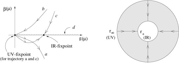
Figure 1: In the left figure, the arrows indicate the IR scaling behaviour of the RG $\beta$-function. Case $a$: There is no IR-fixpoint. At large distances the coupling constant $g$ diverges, but it is UV-free. Case $b$: Is the opposite, in the UV limit the coupling diverges whereas in the infrared the model is free. Case $c$: This is a model with two fixpoints and finally case $d$ shows a model where the $\beta$ function vanishes identical. The right figure shows the corresponding $AdS$ picture, where the different cases are related to singular or regular behaviour near the inner boundary (horizon).

What does this fixpoint behaviour mean for the $AdS$ picture? An obvious possibility to implement this behaviour is to consider a non-trivial background, which “creates” a second boundary of the $AdS$ space and allows unbroken supersymmetries. Again, on this second boundary we may expect that the $AdS$ group is realized as conformal group and therefore, the worldvolume field theory approaches a non-trivial fixpoint. As candidates for this scenario we may take BPS black holes. The asymptotic vacuum translates into the UV fixpoint and moving towards the horizon we approach the IR region of the worldvolume field theory. In the case that the horizon is regular, the moduli will move towards a finite value causing an interacting worldvolume theory at a non-trivial IR fixpoint. On the other hand if the horizon is singular the coupling constant will diverge. This does not necessarily mean that the model does not make sense - it could simply indicate that we have to change the variables. E.g. for the $AdS_{5}$ case: BPS black holes of $N$=4 gauged supergravity should describe RG flow of $N$=2 super Yang-Mills whereas BPS black holes of $N$=2 gauged supergravity correspond to $N$=1 super Yang-Mills. Notice, it is important to consider supersymmetric black holes, the Schwarzschild deSitter black holes will break all supersymmetries and are usually interpreted as adding temperature to a given super Yang Mills theory (with a compact Euclidean time).

One may object that the horizon is not really a boundary in the supergravity sense, by a change of coordinates we can extend the spacetime beyond the horizon. But the same is also true for the field theory, which has also a realization beyond the (non-trivial) fixpoint. However, the system is trapped between two fixpoints under the RG flow. In order to cross the horizon one has to change the coordinate system (e.g. Kruskal coordinates), which translates into field theory in a change of operators, especially the Hamiltonian describing the evolution in a given time has to be changed. But when formulated in the asymptotic flat coordinate system it is the maximal extendable region, see also [6].

It is the aim of this letter to discuss this scenario in more detail. We will start with the $AdS_{3}$ case and investigate the outer region of BTZ black hole [7]. In order to extract the different CFTs it is natural to employ the Chern-Simons formulation of 3-d gravity [8], [9], which makes the holographic nature manifest. It is also worth to mention that in this setup it is important that the BTZ black hole represents a discrete identification along one of the $AdS$ Killing vectors. This construction devides the $AdS$ space in different domains [10] and our annulus is one of them. Furthermore, we will show in section 2.1 that the BTZ black hole can be recast into a domain wall interpolating between an asymptotic $AdS$ vacuum and a flat space with a linear dilaton. Using the Chern-Simons setup for the $AdS$ vacuum we will give a derivation of the CFTs in section 2.2. Finally, in section 3 we turn to the $AdS_{5}$ case, where the situation is much more involved. We will focus on the question how we can break supersymmetry by adding various types of BPS black holes, corresponding to $N$=2 or $N$=1 super Yang Mills as worldvolume theory.

2 The joy at $AdS_{3}$

A good starting point is to describe the situation for $AdS_{3}$ gravity and we are interested in a background with the 2-d spatial geometry given by an annulus. A natural candidate for this is the outer region of the BTZ black hole [7]. Before we discuss the CFTs near the boundaries it is usefull to discuss the black hole and their dual string (=domain walls) as solutions of 3-d gravity.

2.1 3-d gravity: black holes and domain walls

The BTZ black hole is given by

$$ds^{2}=-e^{-2V(r)}\ dt^{2}+e^{2V(r)}\ dr^{2}+\Big{(}{r\over l}\Big{)}^{2}\ \Big{(}dy-\frac{r_{-}r_{+}}{r^{2}}\,dt\Big{)}^{2}$$ (1)

with

$$e^{-2V(r)}={(r^{2}-r_{-}^{2})(r^{2}-r_{+}^{2})\over r^{2}l^{2}}$$ (2)

The horizons of the BTZ black hole are located at $r=r_{\pm}$, the mass and angular momentum are given by $M={r_{+}^{2}+r_{-}^{2}\over l^{2}}$ and $J={2r_{+}r_{-}\over l^{2}}$. It solves the equations of motion coming from the three-dimensional action

$$S=\frac{1}{2\kappa_{3}^{2}}\int\ d^{3}x\ \sqrt{-g}\ (R\ +\ {2\over l^{2}})$$ (3)

where the cosmological constant $l$ is given by the $AdS$ radius. Since we are in 3 dimensions we can dualize the cosmological constant to an antisymmetric tensor

$$S=\frac{1}{2\kappa_{3}^{2}}\int\ d^{3}x\ \sqrt{-g}\ (R\ -\ {1\over 12}H^{2})$$ (4)

with

$$H^{\mu\nu\rho}={2\over l}\,{1\over\sqrt{g}}\epsilon^{\mu\nu\rho}\qquad\qquad(B_{0y}={r^{2}\over l^{2}})\ .$$ (5)

This indicates that there is a dual domain wall solution, which is a string in 3 dimensions. In fact $T$-dualizing the $y$ direction one obtains

$$\begin{array}[]{l}ds^{2}=\left({r_{-}^{2}+r_{+}^{2}\over l^{2}}-{r_{-}^{2}r_{+}^{2}\over l^{2}r^{2}}\right)\,dt^{2}-2\,dtdy+{l^{2}\over r^{2}}dy^{2}+e^{2V}dr^{2}\ ,\\ e^{-2\phi}={r\over l}\qquad,\qquad B={r_{-}r_{+}\over r^{2}}dt\wedge dy\ .\end{array}$$ (6)

Depending on the extreme or non-extreme case one can simplify this solution further; see [11], [12]. For the non-extreme case, we define new coordinates by

$$t\rightarrow{l\over\sqrt{r_{+}^{2}-r_{-}^{2}}}(y-t)\quad,\quad y\rightarrow{1\over l\sqrt{r_{+}^{2}-r_{-}^{2}}}(r_{-}^{2}y-r_{+}^{2}t)\quad,\quad r^{2}\rightarrow r^{2}+r_{-}^{2}$$ (7)

and find (after a gauge transformation in $B\rightarrow B-{r_{-}\over r_{+}}$)

$$ds^{2}={1\over H}\left[-(1-{\mu\over r^{2}})dt^{2}+dy^{2}\right]+{l^{2}\over r^{2}}{dr^{2}\over 1-{\mu\over r^{2}}}\quad,\quad e^{-2\phi}={r^{2}\over l^{2}}\,H\quad,\quad B={r_{-}\over r_{+}H}dy\wedge dt$$ (8)

with $H=1+{r_{-}^{2}\over r^{2}}$. It is interesting to note, that by a further redefinition of the radial coordinate $r^{2}=\mu\cosh^{2}\lambda/l$ we get the metric

$$ds^{2}=-{r_{+}^{2}-r_{-}^{2}\over r_{+}^{2}\coth^{2}\lambda/l-r_{-}^{2}}dt^{2}\ +\ d\lambda^{2}\ +\ {(r_{+}^{2}-r_{-}^{2})\coth^{2}\lambda/l\over r_{+}^{2}\coth^{2}\lambda/l-r_{-}^{2}}dy^{2}$$ (9)

which after compactification over $y$ is exactly the 2-d black hole discussed as in [13]. There is however an important difference to this exact 2-d string background, namely the non-trivial antisymmetric tensor, which becomes a gauge field upon dimensional reduction. Near the boundary at $\lambda=0$ however the $B$ field drops out and the solution coincides with the known exact string background.

For the extreme case ($r_{-}^{2}=r_{+}^{2}=r_{0}^{2}$) we choose the coordinates

$$t\rightarrow{l^{2}\over 2r_{0}^{2}}v\qquad,\qquad y\rightarrow{1\over 2}\left(v-{2r_{0}^{2}\over l^{2}}u\right)\qquad,\qquad r^{2}\rightarrow r^{2}+r_{0}^{2}$$ (10)

and obtain

$$ds^{2}={1\over H}\left[dudv+{r_{0}^{4}/l^{2}\over r^{2}}du^{2}\right]+{l^{2}\over r^{2}}\,dr^{2}\quad,\quad e^{-2\phi}={r^{2}\over l^{2}}H\quad,\quad B={1\over 2H}du\wedge dv$$ (11)

with $H=1+{r_{0}^{2}\over r^{2}}$. Note, in order to go from the non-extreme to the extreme string solution one has first to perform the Lorentz rotation that is included in the transformation (7) and afterwords make the standard extreme limit.

In addition, the BTZ black hole itself can be written as a string solution. Defining a new radius in the extreme case ($r_{+}=r_{-}=r_{0}$) by

$$r^{2}\rightarrow r^{2}+r_{0}^{2}$$ (12)

the BTZ black hole (1) becomes

$$ds^{2}={r^{2}\over l^{2}}\left[dudv+{r_{0}^{2}\over r^{2}}du^{2}\right]+{l^{2}\over r^{2}}dr^{2}$$ (13)

where $v/u=y\pm t$. Both (extreme) string solutions have an important difference: they corresponds to different asymptotic vacua. The solution given in (11) is asymptotically flat with a linear dilaton background

$$ds^{2}=dudv+{l^{2}\over r^{2}}dr^{2}=dudv+d\lambda^{2}\quad,\quad\phi=-{1\over l}\,\lambda$$ (14)

where the background charge is given by the $AdS$ radius. Hence, in the asymptotic vacuum ($\lambda\rightarrow\infty$) we are in a weakly coupled region. On the other hand the dual string in (13) is asymptotically anti-de Sitter

$$ds^{2}={r^{2}\over l^{2}}dudv+{l^{2}\over r^{2}}dr^{2}\ .$$ (15)

with vanishing (or fixed) dilaton. Anti-deSitter gravity in 3 dimensions exhibits holography, which becomes manifest if one formulate it as a topological Chern-Simons model. As consequence, also the dual model with a linear dilaton background has to show holography, see also [15].

Notice, near the core ($r\simeq 0$) both solutions (11) and (13) are equivalent and we may identify and see them as as two sides of a domain wall, see figure 2.

Figure 2: It shows the domain wall solution. On one side we have the $AdS_{3}$ vacuum and the solution is given by (13). On the other side we have a linear dilaton vacuum and the solution corresponds to (11). The coupling constant is fixed on the $AdS$ side whereas it vanish in the linear dilaton vacuum. Both sides are dual to each other.

2.2 Conformal field theories of $AdS_{3}$ gravity

Let us come back to the $AdS$ side in figure 2 and let us determine the CFTs. It is known that Einstein-anti-de Sitter gravity in $2+1$ dimensions as given by the action (3) is equivalent to a Chern-Simons theory [8], [9]. Choosing conventions where the three-dimensional gravitational coupling is related to the level $k$ by

$$k=\frac{2\pi l}{\kappa^{2}_{3}}$$ (16)

and decomposing the diffeomorphism group $SO(2,2)\simeq SL(2,{\bf R})_{L}\times SL(2,{\bf R})_{R}$ the 3-dimensional action can be written as

$$S=S_{CS}[A]\ -\ S_{CS}[\bar{A}]$$ (17)

with

$$S_{CS}[A]=\frac{k}{4\pi}\int_{M_{3}}d^{3}x{\rm Tr}\ (AdA+\frac{2}{3}A^{3})\ .$$ (18)

The gauge field one-forms are

$$A=(\omega^{a}+\frac{1}{l}e^{a})\ T_{a}\ \in SL(2,{\bf R})_{R}\ ,\hskip 28.45274pt\bar{A}=(\omega^{a}-\frac{1}{l}e^{a})\ \bar{T}_{a}\ \in SL(2,{\bf R})_{L}.$$ (19)

where $\omega^{a}\equiv\frac{1}{2}\epsilon^{abc}\omega_{bc}$ are given by the spin-connections $\omega_{bc}$ and $e^{a}$ are the dreibeine. Considering non-trivial boundaries the Chern-Simons theory is not invariant under gauge transformations and as a consequence gauge degrees of freedom do not decouple and become dynamical on the boundaries. These are the degrees of freedom of the conformal field theories living at the boundaries.

In the following we will discuss this procedure for the BTZ black hole. The geometry of the manifold is $M_{3}={\bf R}\times\Sigma$, where ${\bf R}$ corresponds to the time of the covering space of $AdS_{3}$ and $\Sigma$ represents an “annulus” $r_{+}\leq r<\infty$.

Calculating the gauge connections $A=A^{a}T_{a}$ and $\bar{A}=\bar{A}^{a}\bar{T}_{a}$ for the BTZ solution (1) one finds (for details see [14], [16])

$$\begin{array}[]{l}A=\Big{(}e^{-V}\,T_{0}+{r\over l}(1-{r_{-}r_{+}\over r^{2}})\,T_{1}\Big{)}{dv\over l}+e^{V}(1+{r_{-}r_{+}\over r^{2}})\,T_{2}\ \frac{dr}{l}\ ,\\ \bar{A}=\Big{(}e^{-V}\,T_{0}-{r\over l}(1+{r_{-}r_{+}\over r^{2}})\,T_{1}\Big{)}{du\over l}-e^{V}(1-{r_{-}r_{+}\over r^{2}})\,T_{2}{dr\over l}\ .\end{array}$$ (20)

The corresponding gauge fields strengths for these gauge potentials vanish, i.e. they represent only gauge degrees of freedom

$$\begin{array}[]{l}A=g^{-1}dg\qquad{\rm with:}\quad g=e^{\lambda T_{2}}e^{vT_{1}}\ ,\qquad\sinh\lambda=\,{l\over r_{+}-r_{-}}\,e^{-V}\\ \bar{A}=\bar{g}^{-1}d\bar{g}\qquad{\rm with:}\quad\bar{g}=e^{\lambda T_{2}}e^{uT_{1}}\ ,\qquad\sinh\lambda=\,-{l\over r_{+}+r_{-}}\,e^{-V}\ .\end{array}$$ (21)

In order to extract the CFTs at the boundaries we have to perform two steps: (i) we have to add boundary terms that impose the correct boundary conditions and (ii) we have to mod out the isometry group of the BTZ solution (corresponds to the Killing direction that has been periodically identified in constructing the BTZ black hole).

(i) As dictated by the Chern-Simons solution (20) we will impose as boundary conditions

$$A_{u}=\bar{A}_{v}=0$$ (22)

and therefore we add as boundary term to the action

$$\delta S={k\over 8\pi}\int_{\partial M}Tr(A_{v}A_{u}+\bar{A}_{v}\bar{A}_{u})\ .$$ (23)

Since we have flat gauge connection we insert $A=g^{-1}dg$ and $\bar{A}=\bar{g}^{-1}d\bar{g}$ into the action and one obtains as result an $SL(2,{\bf R})$ WZW model [17].

(ii) The subgroup that has to be modded out can be determined from the Chern-Simons fields (20): for $r\rightarrow\infty$ one finds deformation along $T_{\pm}$ group direction and near the horizon deformations along the spatial $T_{1}$ direction. Notice, that the degrees of freedom of the boundary CFT are the “broken gauge degrees of freedom” (that become dynamical on the boundary) and the isometries represent residual symmetries. To get the right CFT we have to mod out the residual symmetries and hence obtain gauged WZW models. It has been discussed some time ago, that by gauging a lightcone group direction one truncates the $SL(2,{\bf R})$ to a Liouville model and by gauging the spatial direction one obtains a 2-d black hole solution (see [18], [13]), which becomes a string background in the extreme limit.

These CFTs coincides with our expectation from the domain wall discussion, i.e. the Liouville model corresponds to the linear dilaton vacuum, whereas the domain wall itself is described by a 2-d black hole (9) in the non-extreme case or the string solution (11) in the extreme case. Both solution are known to be exact CFTs. In this approach we do not consider the BTZ black hole as small perturbation around the asymptotic vacuum, but as interpolating solution between two CFTs. Due to the holographic nature, the complete bulk physics will be fixed by these boundary CFTs.

Therefore, the outer-CFT is an ${SL(2,{\bf R})\over SO(1,1)}$-WZW model (Liouville model) defined by the 2-d action [13], [14]

$$S={k-2\over 4\pi l^{2}}\int\left[(\partial\lambda)^{2}-Ql\lambda R^{(2)}+\mu e^{-2\lambda/l}\right]$$ (24)

with the level of the WZW model $k={l\over 4\alpha^{\prime}}$ and the background charge $Q={k-1\over k-2}$. The Liouville field $\lambda$ describes radial fluctuations: $e^{-2\lambda/l}=\Big{(}{l\over r}\Big{)}^{2}$ and the central charge of this model is

$$c_{outer}=1+6(k-2)Q^{2}={3k\over k-2}-2+6k\ .$$ (25)

In the classical limit of large $AdS$ radius ($k\rightarrow\infty$) only the last term contributes.

The inner-CFT is the standard ${SL(2,{\bf R})\over U(1)}$ gauged WZW model [18], [13] with the central charge

$$c_{inner}={3k\over k-2}-1\ .$$ (26)

The Lagrangian of this CFT is given by a 2-d $\sigma$-model with background fields given in (8) for the non-extreme case or in (11) for the extreme case. The difference in the central charges indicates that there is no exact marginal deformation connecting the outer and inner CFT. However, let us stress that at any finite point in space time one can promote the background to an exact CFT. On one hand the gauged WZW model can be made exact by changing the renormalization group scheme (field redefinitions) [19] and on the other hand the BTZ black hole is locally at any point $AdS_{3}$. The different central charges indicate the non-trivial global structure of the model and it is better thought of as an interpolating solution between two (different) CFTs.

3 The worry with $AdS_{5}$

The $AdS_{3}$ case was especially simple, mainly because we were dealing with 2-d CFTs, but also, because we did not consider any matter. One may motivate this, because in 3 dimensions gauge fields are dual to scalar fields and since $AdS_{3}$ is typically discussed as the near horizon region of strings all scalars are fixed (they become constant near regular horizon).

For $AdS_{5}$ the situation is much more complicated, not only that we are dealing with 4-dimensional CFTs, but also because we have no reason to ignore matter. Instead we want to use non-trivial gauge fields to break successive supersymmetry. Following the picture described in the introduction we will consider charged BPS black holes that breaks supersymmetry and tries to verify the different cases as shown in figure 1. In this setup the number of unbroken supersymmetries is related to the number of independent charges.

When viewed from a 10-dimensional perspective every charge corresponds to one brane and at least some of them have to intersect in order to break supersymmetry. The single 3-brane, e.g., gives the $AdS_{5}$ vacuum. It breaks half of the 10-d supersymmetry and corresponds thus to $N$=4 super Yang Mills (case $d$ in figure 1). Upon compactification over the spherical part, the 3-brane charge enters the cosmological constant of the $AdS$ space. By adding a further brane we break again one half of supersymmetry, i.e. for the worldvolume theory we expect to get $N$=2 super Yang Mills. In order to reach $N$=1 super Yang Mills we have to consider 3 and 4 charge configurations (typically both cases have the same amount of unbroken supersymmetries).

So, from the 5-dimensional point of view we have to discuss black holes with 1, 2 or 3 independent charges (one charge is absorbed by the cosmological constant). Thus, we consider the $STU$-model for gauged supergravity given by the action

$$S\sim\int\left[{R\over 2}+g^{2}V(X)-{1\over 4}G_{IJ}F^{I}_{\mu\nu}F^{J\,\mu\nu}-{1\over 2}G_{IJ}\partial_{\mu}X^{I}\partial^{\mu}X^{J}\right]+{1\over 48}\int F^{1}\wedge F^{2}\wedge A^{3}$$ (27)

with $(S,T,U)=X^{I}=(X^{1},X^{2},X^{3})$ which have to fulfil the the constraint $STU=1$. The potential and the scalar metric is

$$V(X)=9\;V_{I}V_{J}(X^{I}X^{J}-{1\over 2}G^{IJ})\qquad,\qquad G_{IJ}={1\over 2}\left(\begin{array}[]{ccc}{1\over S^{2}}&&\\ &{1\over T^{2}}&\\ &&{1\over U^{2}}\end{array}\right)$$ (28)

where the constants $V_{I}$ parameterize the $U(1)$ subgroup that has been gauged and $g$ is the corresponding gauge coupling constant, see [20]. A black hole solution for this Lagrangian has recently be found [21] and reads

$$\begin{array}[]{l}ds^{2}=-e^{-4U}fdt^{2}+e^{2U}\left[{dr^{2}\over f}+r^{2}d\Omega_{3}\right]\quad,\quad X^{I}={e^{2U}\over H_{I}}\quad,\quad A^{I}={1\over H_{I}}dt\\ e^{6U}=H_{1}H_{2}H_{3}\qquad,\qquad f=1+g^{2}r^{2}e^{6U}\qquad,\qquad H_{I}=h_{I}+{Q_{I}\over r^{2}}\end{array}$$ (29)

where $Q_{I}$ are the different electric charges of the black hole and the constant parts of the harmonic functions are related to the vector parameterizing the gauged subgroup: $h_{I}=3V_{I}$. If all charges vanish we find the $AdS$ vacuum ($e^{2U}=1$). The asymptotic geometry is $R\times S_{3}$ ($R$ is the time), but it is straightforward to replace the $S_{3}$ with a more general manifold with constant curvature $k$ by

$$d\Omega_{3}\rightarrow d\Omega_{3,k}=d\chi^{2}+\Big{(}{\sin\sqrt{k}\chi\over\sqrt{k}}\Big{)}^{2}\Big{(}d\theta^{2}+\sin^{2}\theta d\phi^{2}\Big{)}\quad,\quad f\rightarrow k+g^{2}r^{2}e^{6U}\ .$$ (30)

As explained before, the number of non-vanishing charges is related to the number of unbroken supersymmetries. The single black hole should be related to $N$=2 super Yang Mills, whereas the double and triple charged case should describe $N$=1 super Yang Mills.

In order to keep the expressions simple let us identify all non-vanishing charges, i.e.  we write

$$e^{6U}=H^{n}=\Big{(}1+{Q\over r^{2}}\Big{)}^{n}$$ (31)

where $n=1,2,3$ counts the number of equalised charges. Introducing a new radius by

$$\rho^{2}=r^{2}+Q$$ (32)

the metric becomes

$$ds^{2}=e^{2V}dt^{2}+e^{-2V}{d\rho^{2}\over\Delta}+\rho^{2}\Delta d\Omega_{3,k}\qquad,\qquad e^{2V}=k\Big{(}1-{Q\over\rho^{2}}\Big{)}^{2n\over 3}+g^{2}\rho^{2}\Delta$$ (33)

with $\Delta=(1-{Q\over\rho^{2}})^{3-n\over 3}$. As discussed in [21] the solution for $k=1$, i.e. eq. (29), is ill-defined. For the three charges case ($\Delta=1$) it has a naked singularity and for one or two charges there is a singular horizon. The best one can get is single charge case where the horizon is infinitely far away (we keep the asymptotic time, see introduction). The situation becomes better for $k=-1$, where a zero of $f$ or $e^{2V}$ indicates a horizon, but in this case the spatial geometry is given by an hyperboloid. Furthermore, interesting to note is the case where the asymptotic space is Minkowskean, i.e. $k=0$, we get back the $AdS$ vacuum for three equal charges (see (33)) and only if the charges are not equal one finds a deformation of the $AdS$ space.

Let us come back to our original motivation, i.e. to get a supergravity picture for the figure 1. By comparing our supergravity solution with the field theory expectations we immediately run into a contradiction, namely we are interested in a model that is UV free. The UV region of the field theory translates into the asymptotic supergravity solution, but all scalar fields are simply constant there and do not vanish. We may “cure” this by setting some of the constants in the harmonic functions ($h^{\prime}s$) to zero, but then we are loosing the asymptotic $AdS$ space. As solution to this problem we will do the same as in the $AdS_{3}$ case: we look for the linear dilaton vacuum, which can directly be translated into field theory. In the domain wall picture, the linear dilaton vacuum should describe the second asymptotic region, see figure 2.

Consider the single charge case where the the metric and scalars read

$$\begin{array}[]{l}ds^{2}=-{1\over H^{2/3}}\,f\,dt^{2}+H^{1/3}\Big{(}{dr^{2}\over f}+r^{2}d\Omega_{3,k}\Big{)}\quad,\quad H=h+{Q\over r^{2}}\\ S=H^{-2/3}\quad,\quad T=U=H^{1/3}\quad,\quad f=(k+g^{2}Q+g^{2}r^{2}h)\ .\end{array}$$ (34)

Notice the constraint $STU=1$ eliminates one scalar, so that there is only one physical scalar either $S$ or $T=U$. Both cases have a different physical interpretation, in one case the gauge field comes from an electric 10-d gauge field whereas the other case comes from a magnetic gauge field (that has been dualized in 5 dimensions). Lets start with the magnetic case, so we dualize the electric gauge field into an antisymmetric tensor and interprete $S$ as our physical scalar (i.e. we have to replace $T$ and $U$ in the action by $T=U=1/\sqrt{S}$). Next, we identify this scalar with the dilaton and find for the string metric

$$ds_{str}^{2}=e^{{4\over 3}\phi}ds^{2}=-fdt^{2}+H\left({dr^{2}\over f}+r^{2}d\Omega_{3,k}\right)\quad,\quad S^{-1}=e^{{4\over 3}\phi}=\Big{(}h+{Q\over r^{2}}\Big{)}^{2/3}\ .$$ (35)

This is a NS5-brane wrapping the 5-d internal space. In order to reach the linear dilaton vacuum we have to enter the throat region, e.g. by considering a large charge $Q$ or equivalently turn off the constant part in the harmonic functions (i.e. $H={Q\over r^{2}}$). Defining a new radius we obtain

$$ds^{2}=-(k+g^{2}Q)\,dt^{2}+{Q\over k+g^{2}Q}\Big{(}{dr\over r}\Big{)}^{2}+Q\,d\Omega_{3,k}\qquad,\qquad e^{2\phi}={Q\over r^{2}}\\$$ (36)

and hence for $k=0$ we get the flat space background with a linear dilaton. How about the dual case, which should be related to a compactified fundamental string? In this case we take $T=U$ as physical scalar and do not dualize the gauge field. As result one gets in the string frame

$$\tilde{d}s_{str}^{2}=e^{{4\over 3}\phi}ds^{2}=-{f\over H}dt^{2}+\left({dr^{2}\over f}+r^{2}d\Omega_{3,k}\right)\quad,\quad T=e^{-{2\over 3}\phi}=\Big{(}h+{Q\over r^{2}}\Big{)}^{1/3}\ .$$ (37)

Again, neglecting the constant part $h$ we find the metric and dilaton

$$\tilde{d}s^{2}=r^{2}\left[-(g^{2}+{k\over Q})\,dt^{2}+d\Omega_{3,k}\right]+{dr^{2}\over k+g^{2}Q}\qquad,\qquad e^{2\phi}={r^{2}\over Q}$$ (38)

which is again flat space for $k=0$, but the dilaton has been inverted in comparison to the case before.

These solutions describe the situation as shown in figure 1(a) and 1(b). For the magnetic case as described by (36) the coupling constant vanish asymptotically ($\phi\rightarrow-\infty$ for $r\rightarrow\infty$) and approaching the core of the solution, i.e. moving towards the IR region, we enter the strongly coupled region ($\phi\rightarrow\infty$ for $r\rightarrow 0$). This is the situation of figure 1(a). On the other hand the trajectory of figure 1(b) corresponds to the electric case as given in (38). In the asymptotic vacuum (UV region) we are in strongly coupled region and approaching the core of the model (IR region) it becomes weakly coupled ($e^{2\phi}\rightarrow 0$).

Of course, one would like to have a similar situation as in the $AdS_{3}$ case, where we had two dual solutions and could identify them as the two sides of a domain wall. Here in $AdS_{5}$, in addition to a symmetry transformation we had to neglect the constant part in the harmonic function. It would be very nice, if one could achieve also this by a symmetry transformation, perhaps along the line of ungauged case as discussed in [23], [24].

4 Conclusions

Employing the AdS/CFT correspondence we made an attempt to find a supergravity setup for the RG flows as shown in figure 1. In this picture the asymptotic $AdS$ configuration translates into the UV region of the worldvolume field theory. We argued, that a BPS black hole with a regular horizon translates into the field theory in an addition IR fixpoint, i.e. the near-horizon CFT is dual to the worldvolume field theory near the the IR fixpoint. Especially we discussed the cases of $AdS_{3}$ and $AdS_{5}$.

For $AdS_{3}$ we considered a domain wall solution, that interpolates between an asymptotic $AdS$ and a linear dilaton vacuum. On the $AdS$ side it is the BTZ black hole and on the other side it is the $T$-dual configuration. The CFT corresponding to the asymptotic vacuum differs from the CFT realized near the horizon. This example should describe the case shown in figure 1(c).

For the $AdS_{5}$ case we discussed examples that describe the situation as shown in figure 1(a) and 1(b). The case (a) is described by a single charged $AdS$ black hole, where the charge comes from a compactified NS5-brane. The case (b) is the dual electric case, i.e. the charge comes from a fundamental string. Like for $AdS_{3}$, for this interpretation we had in both cases to find a flat space description (i.e. the throat region of the 5-brane). This was done by going into the string frame and neglecting the constant part in the harmonic function.

The blowing up of the couplings, either in the UV or IR, can be traced back to the singular horizon of the $AdS$ black hole (34) and indicates that the models are well defined only in certain regions. One may try to improve the situation by adding more charges, but the opposite happens. For the single charge case the singular horizon was infinitely far away, but adding a second charge the singular horizon is at finite distance. This would translate into the RG that the coupling would diverge for a finite value of the RG parameter. In the case of 3 charges the singular horizon dissappears but instead we face a naked singularity (also at finite distance). So, for all these cases the gauge theory should be ill defined and may wonder about the reason. It is very tempting to speculate that the singularities for the double and triple charged black hole are related to anomalies of the gauge theory. Note, in comparison to the $AdS$ vacuum these solutions have only 1/4 of remaining supersymmetries and hence they correspond to $N$=1 super Yang Mills. In contrast, the single charged black hole as discussed before translates into $N$=2 super Yang Mills.

What options do we have to cure this break down? First, one can add higher derivative terms, including e.g. the Gauss-Bonnet term. E.g. in analogy to the $AdS_{3}$ case one can discuss the pure gravity sector in terms of a 5-d Chern-Simons theory. This model contains higher curvature terms and the corresponding black holes are regular, see [25]. We discussed only a pure bosonic supergravity background, a further option would be to include also their fermionic super partners [26]. Since there is no supersymmetry enhancement they will give non-trivial corrections. Finally, the inclusion of rotation may have some attractive features, e.g. one can break supersymmetry already at zero temperature and as claimed in [27], [28] $AdS$ gravity allows for rotating BPS black holes with a regular horizon.

Acknowledgements

I would like to thank Andreas Karch for extensive discussions and Arkady Tseytlin for helpful comments. Research supported by Deutsche Forschungsgemeinschaft (DFG).

References

- [1] H. J. Boonstra, K. Skenderis, and P. K. Townsend, “The domain wall/QFT correspondence,” hep-th/9807137.
- [2] G. W. Gibbons, G. T. Horowitz, and P. K. Townsend, “Higher dimensional resolution of dilatonic black hole singularities,” Class. Quant. Grav. 12 (1995) 297–318, hep-th/9410073.
- [3] J. Maldacena, “The large N limit of superconformal field theories and supergravity,” hep-th/9711200.
- [4] P. Claus, R. Kallosh, and A. V. Proeyen, “M five-brane and superconformal (0,2) tensor multiplet in six-dimensions,” Nucl. Phys. B518 (1998) 117, hep-th/9711161.
- [5] J. Maldacena, “Talk at Strings98,” www.itp.ucsb.edu/online/strings98/maldacena.
- [6] T. Banks, M. R. Douglas, G. T. Horowitz, and E. Martinec, “AdS dynamics from conformal field theory,” hep-th/9808016.
- [7] M. Banados, C. Teitelboim, and J. Zanelli, “The black hole in three-dimensional space-time,” Phys. Rev. Lett. 69 (1992) 1849–1851, hep-th/9204099.
- [8] A. Achucarro and P. K. Townsend, “A Chern-Simons action for three-dimensional anti-de sitter supergravity theories,” Phys. Lett. B180 (1986) 89.
- [9] E. Witten, “(2+1)-dimensional gravity as an exactly soluble system,” Nucl. Phys. B311 (1988) 46.
- [10] M. Banados, M. Henneaux, C. Teitelboim, and J. Zanelli, “Geometry of the (2+1) black hole,” Phys. Rev. D48 (1993) 1506–1525, gr-qc/9302012.
- [11] G. T. Horowitz and D. L. Welch, “Exact three-dimensional black holes in string theory,” Phys. Rev. Lett. 71 (1993) 328–331, hep-th/9302126.
- [12] J. H. Horne and G. T. Horowitz, “Exact black string solutions in three-dimensions,” Nucl. Phys. B368 (1992) 444–462, hep-th/9108001.
- [13] R. Dijkgraaf, H. Verlinde, and E. Verlinde, “String propagation in a black hole geometry,” Nucl. Phys. B371 (1992) 269–314.
- [14] K. Behrndt, I. Brunner, and I. Gaida, “ gravity and conformal field theories,” hep-th/9806195.
- [15] O. Aharony, M. Berkooz, D. Kutasov, and N. Seiberg, “Linear dilatons, NS5-branes and holography,” hep-th/9808149.
- [16] T. Lee, “(2+1)-dimensional black hole and (1+1)-dimensional quantum gravity,” hep-th/9706174.
- [17] S. Elitzur, G. Moore, A. Schwimmer, and N. Seiberg, “Remarks on the canonical quantization of the Chern-Simons-Witten theory,” Nucl. Phys. B326 (1989) 108.
- [18] E. Witten, “On string theory and black holes,” Phys. Rev. D44 (1991) 314–324.
- [19] K. Sfetsos and A. A. Tseytlin, “Antisymmetric tensor coupling and conformal invariance in sigma models corresponding to gauged wznw theories,” Phys. Rev. D49 (1994) 2933–2956, hep-th/9310159.
- [20] M. Gunaydin, G. Sierra, and P. K. Townsend, “Gauging the d = 5 Maxwell-Einstein supergravity theories: More on jordan algebras,” Nucl. Phys. B253 (1985) 573.
- [21] K. Behrndt, A. H. Chamseddine, and W. A. Sabra, “BPS black holes in N=2 five-dimensional AdS supergravity,” hep-th/9807187.
- [22] K. Behrndt and S. Förste, “Cosmological string solutions in four-dimensions from 5-d black holes,” Phys. Lett. B320 (1994) 253–258, hep-th/9308131.
- [23] H. J. Boonstra, B. Peeters, and K. Skenderis, “Duality and asymptotic geometries,” Phys. Lett. B411 (1997) 59, hep-th/9706192.
- [24] E. Bergshoeff and K. Behrndt, “D-instantons and asymptotic geometries,” Class. Quant. Grav. 15 (1998) 1801, hep-th/9803090.
- [25] M. Banados, A. Gomberoff, and C. Martinez, “Anti-de sitter space and black holes,” hep-th/9805087.
- [26] K. Behrndt and R. Reinbacher, “in preparation,”.
- [27] V. A. Kostelecky and M. J. Perry, “Solitonic black holes in gauged n=2 supergravity,” Phys. Lett. B371 (1996) 191–198, hep-th/9512222.
- [28] M. M. Caldarelli and D. Klemm, “Supersymmetry of anti-de sitter black holes,” hep-th/9808097.