Bounce solutions and the transition to thermal hopping in $\varphi^{4}$ theory with a $\varphi^{3}$ term

Abstract

The nature of the transition from quantum tunneling at low temperatures to thermal hopping at high temperatures is investigated in a scalar field theory with cubic symmetry breaking. The bounce solution which interpolates between the zero-temperature and high-temperature solutions is obtained numerically, using a multigrid method. It is found that, for a small value of the symmetry-breaking coupling $f$, the transition is first-order. For higher values of $f$, the transition continues to be first-order, though weakly so.

I. INTRODUCTION

The problem of decay of a metastable state via quantum tunneling has important applications in many branches of physics, from condensed matter to particle physics and cosmology. In the semi-classical approximation, the decay rate per unit volume is given by an expression of the form

$$\Gamma\quad=\quad A\quad e^{-S_{E}},$$ (1)

where $S_{E}$ is the Euclidean action of the bounce: the classical solution of the equation of motion with appropriate boundary conditions. The bounce has turning points at the configurations at which the system enters and exits the potential barrier, and the analytic continuation to Lorentzian time at the exit point gives us the configuration of the system at that point and its subsequent evolution. The solution of the equation of motion looks like a bubble in four dimensional Euclidean space with radius R and thickness proportional to the parameter in the symmetry breaking term. If there is more than one solution satisfying the boundary conditions, the one with the lowest $S_{E}$ will dominate Eq. (1). The prefactor A comes from Gaussian functional integration over small fluctuations around the bounce. The formalism at zero temperature is well known [1, 2]; the least action is given by the bounce which is O(4) invariant [3].

At nonzero temperature, the above formalism has to be modified, since the metastable state can decay due to classical thermal motion. In the context of quantum mechanics, the extension of the formalism to finite temperature was carried out by Affleck [4] . He argued that a second order phase transition from the quantum to the thermal regime takes place at some critical temperature. Chudnovsky [5] showed that this is not always true. Depending on the shape of the potential barrier, the crossover from thermally assisted quantum tunneling to thermal activation at high temperature is either first-order (i.e., the first derivative of $\Gamma$ at the transition temperature is discontinuous) or second-order (i.e., the first derivative of $\Gamma$ is continuous, but the second derivative is discontinuous at the transition temperature).

In the context of quantum field theory, little work has been done to explore the nature of the transition from the quantum regime (zero-temperature) to the thermal regime (high-temperature). Linde [6] suggested that periodic bounces could smoothly interpolate between these two regimes. In this picture, at zero temperature the solution is an O(4) symmetric bubble with a radius R. Up to $T\sim{(2R)}^{-1}$, we have periodic, widely separated bounces, and beyond this temperature they start merging into one another producing what is known as a “wiggly cylinder” solution. As one keeps increasing the temperature these wiggles smoothly straighten out and the solution goes into an O(3) invariant cylinder (independent of Euclidean time $\tau$), which dominates the thermal activation regime.

Garriga [7] extended the work of Chudnovsky by studying bubbles in the thin-wall approximation (TWA) at high and low temperatures, as well as the wiggly cylinder solution at intermediate temperatures. He showed that in the TWA the transition is always first-order. However, although motivated by quantum field theory, this work wan not truly field-theoretical.

Ferrera [8] carried the investigation beyond the domain of validity of the TWA. In fact, this was the first fully field-theoretic investigation of bubble formation at arbitrary temperatures. (Such a study must solve the equation of motion at intermediate temperatures, which requires solving a partial differential equation.) Ferrera studied a model field theory which was $\varphi^{4}$ theory with a symmetry-breaking term of the form $f\varphi$. His result is that only for very large wall thickness (i.e., large $f$) a second-order phase transition takes place, while for all other cases a first-order phase transition occurs.

In an earlier paper [9], we studied phase transitions in two kinds of $\varphi^{4}$ theory, with symmetry-breaking terms proportional to $\varphi$ and $\varphi^{3}$ respectively. We obtained accurate numerical solutions to the equation of motion in the zero- and high-temperature limits, and found that, even for a fairly large value of the $\varphi^{3}$ coupling, the thin-wall approximation (TWA) holds to a few percent. An analytical solution for the bounce was obtained, which reproduces the action in the thin-wall as well as the thick-wall limits. We also investigated the dependence of $T_{\star}$, defined by $S_{4}/S_{3}=1/T_{\star}$, on the dimensionless symmetry breaking parameter $f$. For small $f$, the TWA behavior $T_{\star}\propto f$ is obtained, while at larger values of $f$ there is a smooth departure from this [9].

It has been argued recently that the leading correction to the tree potential due to one-loop effects at finite temperature is proportional to $\varphi^{3}$ rather than $\varphi$ [10]. It therefore becomes natural to investigate $\varphi^{4}$ theory with $\varphi^{3}$ symmetry-breaking at arbitrary temperatures. In the present paper, we undertake such an investigation. Our aim is to obtain the bounce solutions at all temperatures, to compute the action and to determine the nature of the phase transition from quantum tunneling to thermal hopping. Our work therefore follows a parallel track to that of Ferrera [8], and it is of interest to compare the results for the two theories. We find that, for small values of $f$, the action shows a kink when plotted against temperature or its inverse $\beta$. This can be identified as a first-order transition. For larger values of $f$ the transition is weakly first-order. The second-order behavior seen by Ferrera for $f=0.75$ is not seen here.

In Sec. II we review the formalism for bounce solutions at finite temperatures. In Sec. III we discuss our numerical algorithm. In Sec. IV we present our results. Finally, conclusions are presented in Sec. V.

II. FINITE TEMPERATURE BOUNCE
SOLUTIONS IN FIELD THEORY

Let us consider a scalar field theory with a Lagrangian density

$${\mathcal{L}}(\varphi)={1\over 2}({\partial_{\mu}\varphi})^{2}-U(\varphi),$$ (2)

where the potential $U(\varphi)$ has two minima at $\varphi_{-}$ (false vacuum) and $\varphi_{+}$ (true vacuum).

In the semi-classical approximation the barrier tunneling leads to the appearance of bubbles of a new phase with $\varphi=\varphi_{+}$. To calculate the probability of such a process in quantum field theory at zero temperature, one should first solve the Euclidean equation of motion :

$$\partial_{\mu}\partial_{\mu}\varphi={dU(\varphi)\over d\varphi},$$ (3)

with the boundary condition $\varphi\to\varphi_{-}$ as $\vec{x}^{2}+\tau^{2}\to\infty$ , where $\tau$ is the imaginary time. The probability of tunneling per unit time per unit volume will be given by

$$\Gamma=A\quad e{{}^{-S_{E}[\varphi]}},$$ (4)

where $S_{E}[\varphi]$ is the Euclidean action corresponding to the solution of Eq. (3) and given by the following expression :

$$S_{E}[\varphi]=\int d^{4}{x}\left[{1\over 2}({\partial\varphi\over\partial\tau})^{2}+{1\over 2}(\nabla\varphi)^{2}+U(\varphi)\right].$$ (5)

It is sufficient in most cases to restrict ourselves to the O(4) symmetric solution $\varphi(\vec{x}^{2}+\tau^{2})$, since it is this solution that provides the minimum $S_{4}$ of the action $S_{E}[\varphi]$ [3]. In this case Eq. (3) takes the simpler form

$${d^{2}\varphi\over d\rho^{2}}+{3\over\rho}{d\varphi\over d\rho}={dU(\varphi)\over d\varphi},$$ (6)

where $\rho=\sqrt{\vec{x}^{2}+\tau^{2}}$, with boundary conditions

$$\varphi\to\varphi_{-}\quad as\quad\rho\to\infty,\quad{d\varphi\over d\rho}=0\quad at\quad\rho=0.$$ (7)

Now, let us consider the finite temperature case. Following [6], in order to extend the above-mentioned results to nonzero temperature, $T\not=0$, it is sufficient to remember that quantum statistics of bosons (fermions) at $T\not=0$ is equivalent to quantum field theory in the Euclidean space-time, periodic (anti-periodic) in the “time” direction with period $\beta=T^{-1}$. One should use the $T$-dependent effective potential $U(\varphi,T)$ instead of the zero-temperature one $U(\varphi)=U(\varphi,0)$. Instead of looking for O(4)-symmetric solution of Eq. (3), one should look for O(3)-symmetric (with respect to spatial coordinates) solutions, periodic in the “time” direction with period $\beta=T^{-1}$. At sufficiently large temperature compared to the inverse of the bubble radius R at $T=0$, the solution is a cylinder whose spatial cross section is the O(3)-symmetric bubble of new radius $R(T)$. In this case, in the calculation of the action $S_{E}[\varphi]$, the integration over $\tau$ is reduced simply to multiplication by $T^{-1}$, i.e., $S_{E}[\varphi]=T^{-1}\>S_{3}[\varphi]$, where $S_{3}[\varphi]$ is a three-dimensional action corresponding to the O(3)-symmetric bubble:

$$S_{3}[\varphi]=\int d^{3}r\left[{1\over 2}{(\nabla\varphi)^{2}}+U(\varphi,T)\right].$$ (8)

To calculate $S_{3}(\varphi)$ it is necessary to solve the equation

$${d^{2}\varphi\over dr^{2}}+{2\over r}{d\varphi\over dr}={dU(\varphi,T)\over d\varphi}$$ (9)

with boundary conditions

$$\varphi\to\varphi_{-}\quad as\quad r\to\infty,\quad{d\varphi\over dr}=0\quad at\quad r=0.$$ (10)

where now $r=\sqrt{\vec{x}^{2}}$. The complete expression for the probability of tunneling per unit time per unit volume in the high-temperature limit ($T>>R^{-1}$) is obtained in analogy to the one used in [2] and is given by:

$$\Gamma(T)=A(T)\>e^{-S_{3}[\varphi,T]/T}.$$ (11)

At intermediate temperature the action will be given, under the assumption of $O(3)$ symmetry, by

$$S_{E}[\varphi,T]=4\pi\int d\tau\int dr\;r^{2}\left[{1\over 2}{({\partial\varphi\over\partial\tau})^{2}+(\nabla\varphi)^{2}}+U(\varphi,T)\right].$$ (12)

and the equation of motion will be

$${\partial^{2}\varphi\over\partial\tau^{2}}+{\partial^{2}\varphi\over\partial r^{2}}+{2\over r}{\partial\varphi\over\partial r}={\partial U(\varphi,T)\over\partial\varphi},$$ (13)

with boundary conditions

$$\varphi\to\varphi_{-}\quad as\quad r\to\infty,\quad\partial\varphi/\partial\tau=0\quad at\quad\tau=\pm\beta/2,0$$ (14)

where $\beta$ is the period of the solution.

III. ALGORITHM

The aim of this paper is to investigate the nature of the phase transition for $\varphi^{4}$ theory with a $\varphi^{3}$ symmetry-breaking term and compare our results with those of Ferrera [8] who discussed a $\varphi$ symmetry-breaking term.

We start with the following Euclidean action inspired by recent work on temperature-dependent corrections to the tree level potential [10] :

$$S_{E}=4\,\pi\int d\tau\int dr\;r^{2}\left[{1\over 2}{({\partial\varphi\over\partial\tau})^{2}+(\nabla\varphi)^{2}}+U(\varphi)\right].$$ (15)

where $U(\varphi)$ is

$$U(\varphi)={\lambda\over 2}(\varphi^{2}-\mu^{2})^{2}-F\varphi^{3}.$$ (16)

. We rescale the Lagrangian density as

$$\varphi\to\varphi/\mu,\quad r\to r\sqrt{\lambda\mu^{2}},\quad f={F\over{\lambda\mu}}$$ (17)

to get

$$S_{E}={4\,\pi\over\lambda}\int d\tau\int dr\;r^{2}\left[{1\over 2}{({\partial\varphi\over\partial\tau})^{2}+(\nabla\varphi)^{2}}+{1\over 2}(\varphi^{2}-1)^{2}-f\varphi^{3}\right].$$ (18)

The only free parameter in the Lagrangian is $f$. Taking different values of $f$ will give us different shapes of the potential. Hence we will be able to explore the nature of the phase transition for thin as well as for thick walls. The equation of motion now becomes

$${\partial^{2}\varphi\over\partial\tau^{2}}+{\partial^{2}\varphi\over\partial r^{2}}+{2\over r}{\partial\varphi\over\partial r}=2(\varphi^{3}-\varphi)-3f\varphi^{2},$$ (19)

with boundary conditions

$$\varphi\to\varphi_{-}\quad as\quad r\to\infty,\quad\partial\varphi/\partial\tau=0\quad at\quad\tau=\pm\beta/2,0.$$ (20)

To solve Eq. (19) we have used a multigrid algorithm. Multigrid methods were introduced in the 1970s by Brandt [11]. More details are available elsewhere [12, 13].

We have used full weighting injection for the projection operator and second-order polynomial interpolation. For the thin wall we have used fourth order polynomial interpolation since more points are coupled to each other than in the thick-wall case. Since we used the multigrid algorithm (not the full multigrid [12]), we have to start from the finest grid and go down to coarse grids and then up and down till the solution converges. Our finest grid has $513\times 513$ points. We have restricted ourselves to three grids ($513\times 513,\;257\times 257,\;133\times 133$).

As we can see Eq. (19) has a singularity at $r=0$. One way to handle it by using an arbitrary regularization $1/r\to{1/(r+\epsilon)}$ with $\epsilon$ chosen suitably small. This is the method used by Ferrera [14]. We use an alternate method based on L’Hospital’s rule, replacing ${(1/r)\partial\varphi/\partial r}$ at $r=0$ by ${\partial^{2}\varphi/\partial r^{2}}$.

We have started with the zero temperature solution as an initial guess solution, as the zero-temperature equation of motion is one-dimensional and straightforward to solve [9]. We used this one-dimensional solution after putting it in two-dimensional form. After computing the zero-temperature solution by the multigrid method we used it as a guess solution for our first finite-temperature solution. To compute the next finite-temperature solution we used the previous one as input, and so on. We followed this procedure (i.e., continuation in temperature) to cover the whole range of temperatures.

At zero temperature we have used point Jacobi relaxation and at finite temperature we have used line Newton Jacobi relaxation in the $\tau$ direction because as the temperature is increased we have to reduce the step size in the $\tau$ direction and this means that more points in the $\tau$ direction will be coupled than in the other direction.

To solve the equation of motion, we need the value $\varphi_{Tc}$ of the bounce at the center. For this, we chose a trial value $\varphi_{c}$ and kept it fixed through the relaxation process (since otherwise the process is bound to diverge [8]). In the zero- and high-temperature limits, $\varphi{T_{c}}$ was fixed very accurately by solving the one-dimensional equation of motion using a predictor-corrector method and shooting in $\varphi_{c}$ [9]. For multigrid, we have found the same behavior as Ferrera [8], i.e. if we give too high value of $\varphi_{c}$ the multigrid solution diverges while for low enough values it converges. If $\varphi_{c}-\varphi_{Tc}\sim\Delta$, the solution converges to an overall accuracy level of order $\Delta$. We found $\Delta\sim 0.1\%$ which corresponds to a low level of error for the solution. The shooting in $\varphi_{c}$, together with the variable amount of relaxation required, makes the program very CPU-intensive. A typical running time for a single value of temperature is about an hour and a half on an 80586 Pentium machine running at 133 MHz.

A drawback of the multigrid method is that we cannot find the solution at an arbitrary value of temperature. We have a solution only at discrete values of $\beta$. A constant step size in $\beta$ implies the interval between successive temperatures increases as we go to higher temperatures. On the other hand, the $\beta$ step cannot be made very small because of the reasons stated above.

Finally, to compute the action for each solution we have used a two-dimensional Simpson method that can be found in [15].

IV. RESULTS

We have used the algorithm described in the above section for solving the equation of motion

$${\partial^{2}\varphi\over\partial\tau^{2}}+{\partial^{2}\varphi\over\partial r^{2}}+{2\over r}{\partial\varphi\over\partial r}=2(\varphi^{3}-\varphi)-3f\varphi^{2}.$$ (21)

To be able to compare our results with Ferrera [8], we have chosen the same three values of the parameter $f$. The first value is $f=0.25$. From [9], $f=0.25$ is within the domain of validity of the TWA Fig. 1 represents the shape of the potential for $f=0.25$. If we compare the action of the zero- and high-temperature solutions with the one-dimensional one, we find a difference of order $0.2\%$. At intermediate temperatures the highest difference is about $0.9\%$. Fig. 2 shows a plot of $S(T)~{}vs~{}\beta$. From it, the value of $\beta$ at which the transition takes place is approximately 21.15 in our dimensionless units. Garriga [7] has shown that, in the TWA, the period at which the transition takes place is given by

$$\beta_{c}={{27\pi}\over 32}R,$$ (22)

where $R$ is the radius of the one-dimensional zero-temperature solution. We have measured the radius from the center of the bounce to the middle of the wall where the absolute first derivative of the field is maximum. Using Eq. (22), we obtain a value of $\beta_{c}\approx 21.205$. The difference between the numerical result and the analytic one is about $0.2\%$, which lies within our estimation of errors. Clearly it is a first-order phase transition and this will always happen as long as the thickness of the wall is much smaller than the radius of the nucleated bubble. Fig. 3(a) shows the zero-temperature solution. We can see that the wall thickness is much smaller than the radius. Fig. 3(b) shows the solution at $\beta=25.3$. We can see that the two bubbles are far from touching each other. Fig. 3(c) shows the solution at $\beta=\beta_{c}$. In this case we can see that the two bubbles just fit within the period. Finally, Fig. 3(d) shows the solution at $\beta\leq\beta_{c}$.

The second value is at $f=0.55$. Fig. 4 shows the shape of the potential. It is clear from the figure that the TWA is not valid since the energy difference between the false and true vacua is larger than the hump at the origin. Fig. 5 shows a plot of $S(T)~{}vs~{}\beta$. From the figure, we can see that the action is constant till $\beta=14.4$ and after that it starts decreasing slowly till it matches with the $\beta S_{3}$ curve, where $S_{3}$ is the high temperature action. The transition point is at $\beta=9.3$. If $f=0.55$ were within the TWA, then the transition point would be at $\beta{{}_{\star}}=9.9$. We can see that the transition point is at a period less than $\beta{{}_{\star}}$. Fig. 6(a) shows the zero-temperature solution. Fig. 6(b) shows the solution at $\beta=14.4$, where the two bubbles have not started touching each other. Hence we have constant action till that period. Fig. 6(c) shows the solution at $\beta=9.3$. We can see that the solution looks like a wiggly cylinder but it is far from a static one, so we still do have a first-order phase transition, but more weakly than for $f=0.25$. Finally, Fig. 6(e) shows the solution at $\beta\leq 9.3$.

Finally, Fig. 7 shows the shape of the potential for $f=0.75$. Fig. 8 shows a plot of $S(T)~{}vs~{}\beta$. From the figure we can see that the action is constant till $\beta=10.3$. After that it starts decreasing till it crosses the $\beta S_{3}$ curve at $\beta=6.25$. Again, if $f=0.75$ were within the TWA, then the crossing point would be at $\beta{{}_{\star}}=7.45$ . The transition point is at $\beta=6.25$, which is again less than $\beta{{}_{\star}}$. Fig. 9(a) shows the zero-temperature solution. Fig. 9(b) shows the solution at $\beta=10.3$; we can see that wiggly cylinder solution has not started forming yet. Fig 9(c) shows the solution at the transition point $\beta=6.25$. We can see that the wiggly cylinders are formed and still far from a static solution. Hence we have a first-order phase transition but more weakly than for $f=0.55$. Finally, Fig. 9(d) shows the solution at $\beta\leq 6.25$.

V. CONCLUSIONS

In this paper we have tried to find out whether the phase transition from the quantum regime to the high-temperature regime is of first or second order for $\varphi^{4}$ theory with a $\varphi^{3}$ symmetry-breaking term. We have investigated three values of $f$. We find that for $f=0.25$ we have a first order phase transition. For $f=0.55$, the transition is still first-order but weaker than for $f=0.25$. Another feature is that the transition point $\beta_{c}$ is less than the point $\beta_{\star}$ where the zero-temperature solution will match the high temperature one. The final value is $f=0.75$. Here we have a weak first order phase transition. Again $\beta_{c}<\beta_{\star}$. In this case the departure is more than for $f=0.55$. So, up to $f=0.75$ we have a first-order phase transition, which is different from what Ferrera [8] found for $f=0.75$. We conclude that, for the potential with a $\varphi^{3}$ symmetry-breaking term, a true second-order phase transition is not seen even at $f=0.75$. This can be understood as follows. A second-order phase transition only occurs when the hump in the potential disappears. In [9] we found that for $\varphi$ symmetry breaking the hump in $U(\varphi$) disappears for $f>0.77$, while for $\varphi^{3}$ it disappears only asymptotically in $f$. The two forms of the potential can be mathematically transformed into each other [16]. However, this obscures the physical meaning of the asymmetry coefficient $f$, so we work with the untransformed potential.

We find that the departure of the transition point ($\beta_{c}$) from the point where O(4) and O(3) match ($\beta_{\star}$) is higher for higher values of $f$. This is expected since, in the domain of validity of the TWA, the surface tension of the bubble is independent of the temperature [9]; hence we must have $\beta_{c}=\beta_{\star}$. Beyond the TWA, on the other hand, we can expect departure from this equality.

Finally, in this paper we have studied a zero-temperature potential motivated by the finite-temperature effective potential [10]. We have incorporated the temperature only in the boundary conditions. In an exact calculation, of course, we should use the full temperature-dependent effective potential. However, we expect that there will be a range of temperatures and parameter values for which the potential of Eq. (16) will be a good approximation to the full potential. Hence, our conclusions about the nature of the transition to the thermal hopping may have relevance to actual physical situations, in particular inflationary cosmology and baryogenesis.

Figure Caption

FIG. 1. Shape of the potential for $f=0.25$.

FIG. 2. Temperature dependence of the Euclidean action: $S(T)vs\beta$ for $f=0.25$.

FIG. 3. Bounce solution for $f=0.25$. $(a)$ $T=0$, $(b)$ $\beta=25.3$,

$(c)$ $\beta=21.15$, and $(d)$ high temperature.

FIG. 4. Shape of the potential for $f=0.55$.

FIG. 5. Temperature dependence of the Euclidean action: $S(T)vs\beta$ for $f=0.55$.

FIG. 6. Bounce solution for $f=0.55$. $(a)$ $T=0$, $(b)$ $\beta=14.4$,

$(c)$ $\beta=9.3$, and $(d)$ high temperature.

FIG. 7. Shape of the potential for $f=0.75$.

FIG. 8. Temperature dependence of the Euclidean action: $S(T)vs\beta$ for $f=0.75$.

FIG. 9. Bounce solution for $f=0.75$. $(a)$ $T=0$, $(b)$ $\beta=10.3$,

$(c)$ $\beta=6.25$, and $(d)$ high temperature.

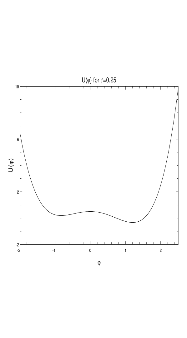
Figure 1:

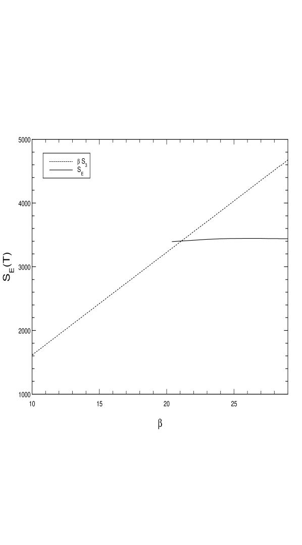
Figure 2:

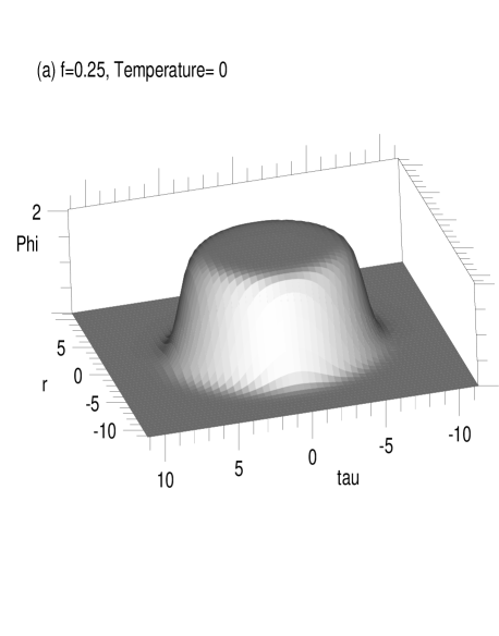
Figure 3:

Figure: 3 (a)

Figure: 3 (b)

Figure: 3 (c)

Figure: 3 (d)

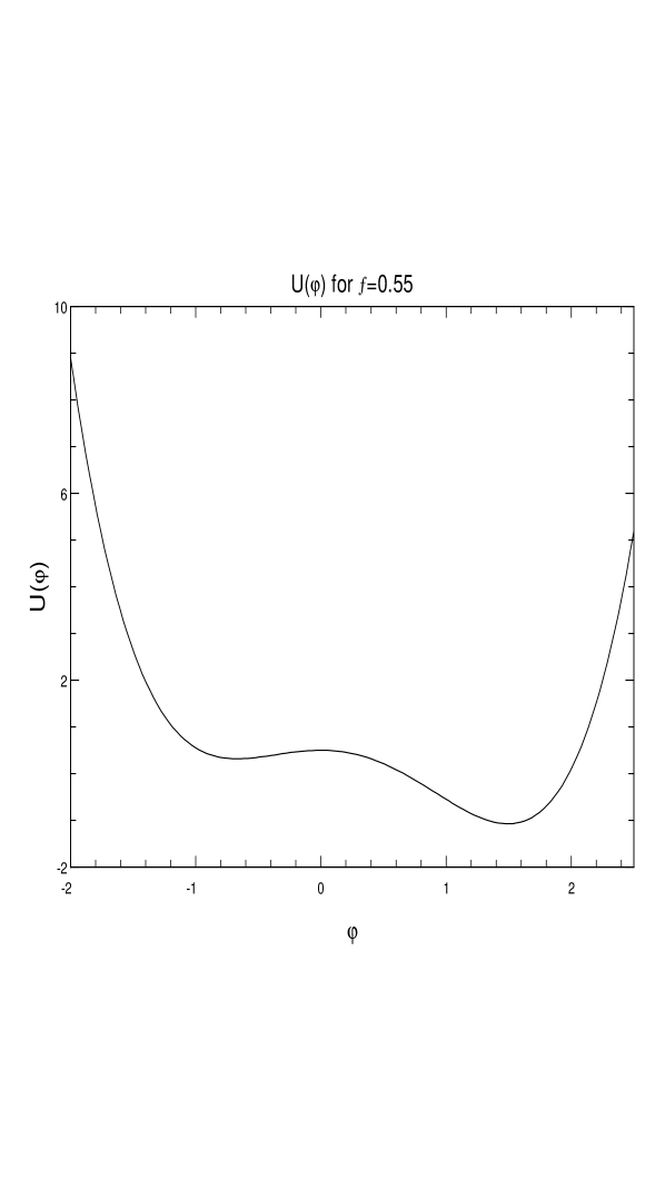
Figure 4:

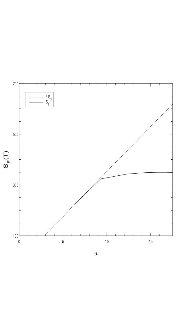
Figure 5:

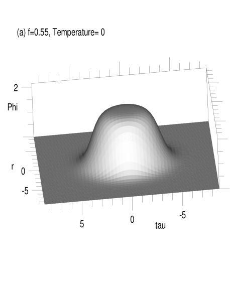
Figure 6:

Figure: 6 (a)

Figure: 6 (b)

Figure: 6 (c)

Figure: 6 (d)

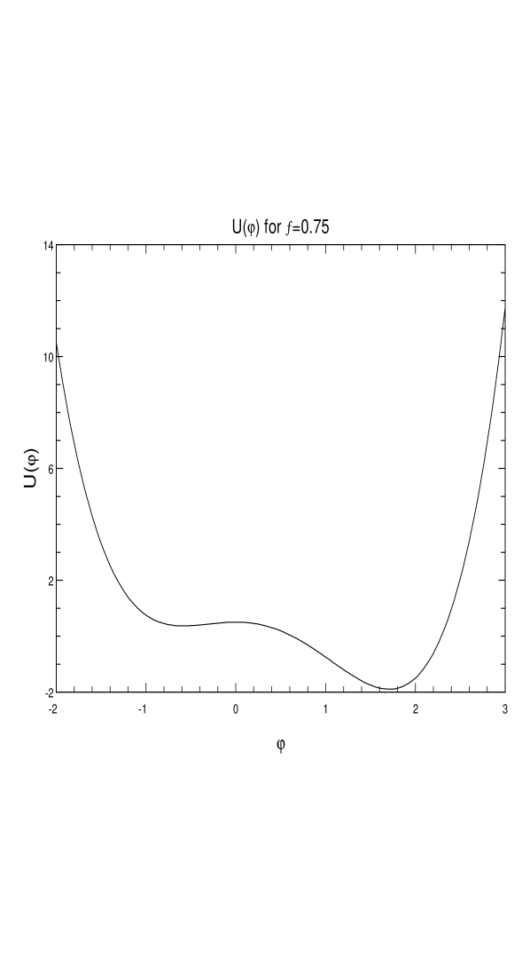
Figure 7:

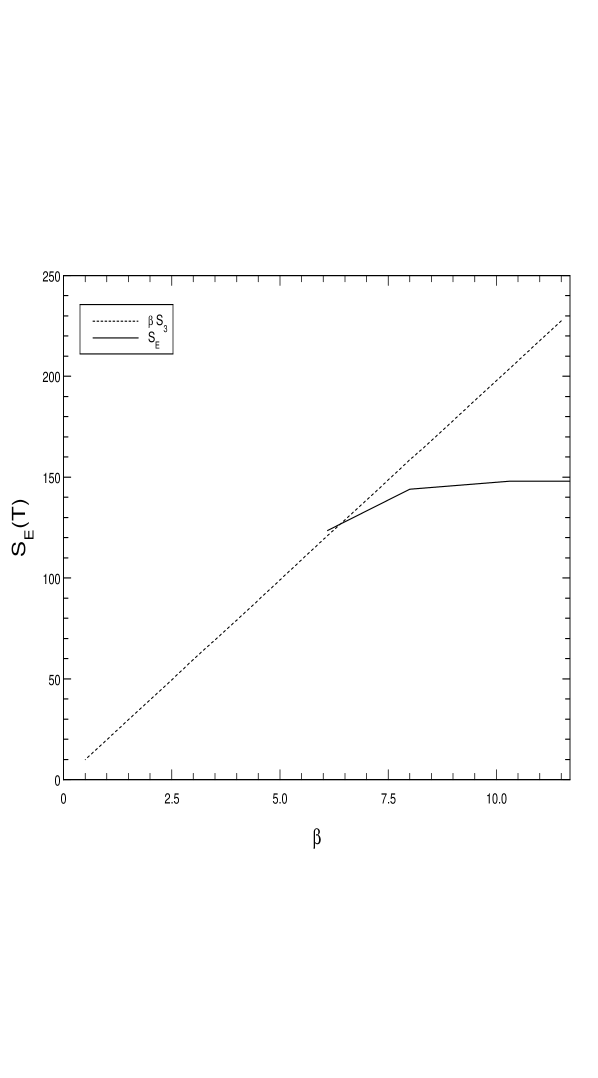
Figure 8:

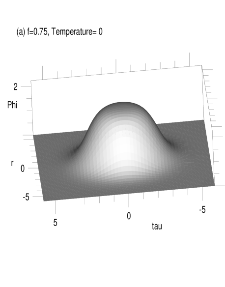
Figure 9:

Figure: 9 (a)

Figure: 9 (b)

Figure: 9 (c)

Figure: 9 (d)

References

- [1] J. S. Langer, Ann. Phys. (N.Y.) 41, 108 (1967).
-
[2]
S. Coleman, Phys. Rev. D 15 2929 (1977).
C. Callan and S. Coleman, Phys. Rev. D 16 1762 (1977).
For a review of instanton methods and vacuum decay at zero temperature, see, e.g., S. Coleman, Aspects of Symmetry (Cambridge University Press, Cambridge, England 1985). - [3] S. Coleman, V. Glaser and A. Martin, Comm. Math. Phys. 58, 211 (1978).
- [4] I. Affleck, Phys. Rev. Lett. 46, 388 (1981).
- [5] E. M. Chudnovsky, Phys. Rev. A 46, 8011, (1992)..
- [6] A. D. Linde, Nucl. Phys. B216, 421 (1983); Particle Physics and Inflationary Cosmology (Harwood Academic Publishers, Chur, Switzerland, 1990).
- [7] J. Garriga, Phys. Rev. D 49, 5497 (1994).
- [8] A. Ferrera, Phys.Rev. D 52, 6717 (1995).
- [9] Hatem Widyan et al (submitted to Phys. Rev. D, hep-th/9803089)
-
[10]
M. Dine, R. Leigh, P. Huet, A. Linde, and D. Linde,
Phys. Rev. D.46, 550 (1992);
G. Anderson and L.Hall, ibid. 45, 2685 (1992);
M. E. Carrington, ibid. 45, 2933 (1992). - [11] A. Brandt, Math. Comput. 31, 333 (1977).
- [12] W. H. Press, S. A. Tuekolsky, W. T. Vetterling, and B. P. Flannery, Numerical Recipes in Fortran (Cambridge University Press, Cambridge, England, 1992).
- [13] W. Hackbusch, Multi-Grid Methods and Applications (New-York: Springer-Verlag, 1985).
- [14] A. Ferrera, private communication.
-
[15]
Handbook of Mathematical Functions
with Formulas, Graphs, and Mathematical Tables
edited by M. Abramowitz and I. A. Stegun (Dover Publications inc. New York, 1972). - [16] F. C. Adams, Phys. Rev. D.48, 2800 (1993).