On confinement in a light-cone Hamiltonian for QCD

Abstract

The canonical front form Hamiltonian for non-Abelian SU(N) gauge theory in 3+1 dimensions and in the light-cone gauge is mapped non-perturbatively on an effective Hamiltonian which acts only in the Fock space of a quark and an antiquark. Emphasis is put on the many-body aspects of gauge field theory, and it is shown explicitly how the higher Fock-space amplitudes can be retrieved self-consistently from solutions in the $q\bar{q}$-space. The approach is based on the novel method of iterated resolvents and on discretized light-cone quantization driven to the continuum limit. It is free of the usual perturbative Tamm-Dancoff truncations in particle number and coupling constant and respects all symmetries of the Lagrangian including covariance and gauge invariance. Approximations are done to the non-truncated formalism. Together with vertex as opposed to Fock-space regularization, the method allows to apply the renormalization programme non-perturbatively to a Hamiltonian. The conventional QCD scale is found arising from regulating the transversal momenta. It conspires with additional mass scales to produce possibly confinement.

1 Introduction

Over the past twenty years two fundamentally different pictures of hadrons have developed. One, the constituent quark model is closely related to experimental observation and phenomenology, see for example goi85 ; dkm91 ; neu93 ; eiq94 and the references cited there. The other, quantum chromodynamics (QCD) is based on a covariant non-abelian quantum field theory. How can one reconcile such models with the need to understand hadronic structure from a covariant theory?

Since “the Hamiltonian is of central importance in usual quantum mechanics” fey48 , an intuitive approach for solving relativistic bound-state problems would be to solve the gauge-fixed Hamiltonian eigenvalue problem. But the presence of the square root operator in the equal-time Hamiltonian approach presents severe mathematical difficulties. Even if these problems could be solved, the eigensolution is only determined in its rest system. Boosting such a wavefunction from the hadron’s rest frame to a moving frame is as complex a problem as solving the bound state problem itself. This reflects the contemporary conviction that the concept of a Hamiltonian is old-fashioned and littered with all kinds of almost intractable difficulties. Alternative procedures like those of Schwinger and Dyson or of Bethe and Salpeter are not easy to cope with either in practice, see for example lsg91 .

So, why does one not proceed with the only successful non-perturbative approach to gauge field theory, with lattice gauge theory fey48 ; wei94 and its recent quantitative predictions nrq95 ?

It is the concept of a wavefunction which is so appealing in an Hamiltonian approach, particularly if one chooses the front form of Hamiltonian dynamics dir49 . The light-cone wavefunctions encode the hadronic properties in terms of their quark and gluon degrees of freedom, and thus all hadronic properties can be derived from them. One can compute electro-magnetic and weak form factors rather directly from an overlap of light-cone wavefunctions leb80 , see also bpp97 , and the hadron and nuclear structure functions are comparatively simple probability distributions. Lattice gauge theory has still a long way to go to formulate such dynamical aspects.

As recently reviewed bpp97 , one has several reasons wil89 why the front form of Hamiltonian dynamics is one of the very few candidates for getting wave functions, see also brp91 ; gla95 . Particularly the simple vacuum and the simple boost properties confront with the complicated vacuum and the complicated boosts in the conventional Hamiltonian theory. Based on the recognition that “the only truly successful approach to bound states in field theory has been quantum electrodynamics (QED) with its combination of non-relativistic quantum mechanics to handle bound states and perturbation theory to handle relativistic effects” wwh94 , Wilson and collaborators wwh94 have proposed a scheme in which one presumes a potential for the bound-states and handles the relativistic effects by structures imposed by the needs of renormalization. This scheme continues to develop gla97 . The only available numerical examples brp95 ; bpw97 ; jop96b however violate each and every symmetry of the Lagrangian.

The aim and motivation of the present work is similar to wwh94 . One aims at finding an effective interaction between quarks in analogy to the Coulomb potential as a crude and zero-order approximation to a given Lagrangian which can be used as a starting point for more refined considerations within a Hamiltonian approach.

But the problems one faces with a Hamiltonian are stupendous. One has to deal with many difficult aspects of the theory simultaneously: confinement, vacuum structure, spontaneous breaking of chiral symmetry (for massless quarks), and describing a relativistic many-body system with unbounded particle number. The problem in non-Abelian gauge theory is compounded not only by the physics of confinement, but also by the fact that the wave function of a composite of relativistic constituents has to describe systems of an arbitrary number of quanta with arbitrary momenta and helicities.

For example, the vacuum in the front form is not truly simple hks92 ; vap92 but still simpler than in the instant form. The problem can at least be formulated in terms of the ‘zero modes’, the space-like constant field components defined in a finite spatial volume. The original conjecture that zero modes represent long range aspects and thus confinement kpp94 , however has not materialized kal96 . Zero modes are important for a ‘theory of the vacuum’, but probably less for the massive part of the spectrum. In the present work zero modes will therefore be suppressed without any good argument other than simplicity. With similar arguments all aspects of chiral symmetry (breaking) are disregarded.

One addresses thus to find the bound-state structure of the light-cone Hamiltonian in the light-cone gauge $A^{+}=0$. This gauge is kind of natural to the light cone, and it is physical since the gluons have only two transverse degrees of freedom. Simple considerations show why other than in 1+1 dimensions one should not address to solve the full Hamiltonian bpp97 in physical space-time. In the first place one should address to develop a well-defined effective interaction, such one as proposed for example by Tamm tam45 and independently by Dancoff dan50 , in their paradigmatic treatment of the Yukawa model. But if one does so and adapts the Tamm-Dancoff approach to the light-cone kpw92 , one finds no trace of a possible confinement in these ‘mesons’. This is rather disturbing since the same approach applied to positronium yields the Bohr aspects of the spectrum including the correct fine and hyperfine splittings.

The Tamm-Dancoff approach will be re-analyzed in Sect. 4. The problems are generic, since for the purpose of practical calculations one must truncate at the lowest non-trivial order of a perturbative series. If one tries to correct for that one gets into all kinds of difficulties including the question how one should resume perturbative series to all orders without double counting. The problem is a severe one since one is forced to mistreat precisely all those multi-particle configurations which one thinks are important for confinement in a field theory. Quite naturally, they come in certain higher powers of the coupling constant and are thrown away when one truncates the perturbative series. In a way that part of the problem is similar to throwing away many-body amplitudes in conventional many-body problems. The problem in field theory are accentuated by the fact that the terms of higher order in the coupling constants are to be multiplied with very large numbers.

The shortcomings of the Tamm-Dancoff approach are overcome here by the method of iterated resolvents pau93 ; pau96a ; pau96 . This novel method is inspired by the Tamm-Dancoff approach and requires the development of a considerable formal apparatus. As to be shown, it allows for a systematic discussion of the many-body effects in a field theory without truncating the expressions at a finite order of perturbation theory, at any time. With only a few well localizable assumptions one ends up with integral equations, whose structure is similar what was solved already in the past kpw92 ; pam95 ; trp96 . Most importantly one arrives at the conclusion that the effective interaction has essentially only two contributions: a flavor-conserving and a flavor-changing part. In a diagrammatical representation both look like low order perturbative graphs. In an approximative sense they even are identical with perturbative graphs, with one important difference however: All genuine many-body effects reside in the effective coupling constant and generate a dependence on the momentum transfer across the vertex. They generate new interactions and possibly generate confinement.

2 The light-cone Hamiltonian (matrix)

The advantages and challenges of quantizing field particularly gauge field theory ‘on the light cone’ and of solving the bound state problem for quantum chromodynamics (QCD) have been reviewed recently bpp97 . It should suffice therefore to recall here the most elementary facets and to shape some notational aspects in short.

Table 1: The Fock space and the Hamiltonian matrix $H^{\prime}=T+V$ for a meson at fixed value of $K=4$. — See discussion in the text. The diagonal blocks are denoted by $T$. Most of the block matrices are zero matrices, marked by a dot ($\cdot$). The block matrices marked by $V$ are potentiall non-zero due to the vertex interaction.

Np

2

2

3

4

3

4

5

6

4

5

6

7

8

K

Np

Sector

n

1

2

3

4

5

6

7

8

9

10

11

12

13

1

2

$q\bar{q}\,$

1

T

$\cdot$

V

$\cdot$

$\cdot$

$\cdot$

$\cdot$

$\cdot$

$\cdot$

$\cdot$

$\cdot$

$\cdot$

$\cdot$

2

2

$g\ g\$

2

$\cdot$

T

V

$\cdot$

V

$\cdot$

$\cdot$

$\cdot$

$\cdot$

$\cdot$

$\cdot$

$\cdot$

$\cdot$

2

3

$q\bar{q}\,\ g$

3

V

V

T

V

$\cdot$

V

$\cdot$

$\cdot$

$\cdot$

$\cdot$

$\cdot$

$\cdot$

$\cdot$

2

4

$q\bar{q}\,q\bar{q}\,$

4

$\cdot$

$\cdot$

V

T

$\cdot$

$\cdot$

V

$\cdot$

$\cdot$

$\cdot$

$\cdot$

$\cdot$

$\cdot$

3

3

$g\ g\ g$

5

$\cdot$

V

$\cdot$

$\cdot$

T

V

$\cdot$

$\cdot$

V

$\cdot$

$\cdot$

$\cdot$

$\cdot$

3

4

$q\bar{q}\,\ g\ g$

6

$\cdot$

$\cdot$

V

$\cdot$

V

T

V

$\cdot$

$\cdot$

V

$\cdot$

$\cdot$

$\cdot$

3

5

$q\bar{q}\,q\bar{q}\,\ g$

7

$\cdot$

$\cdot$

$\cdot$

V

$\cdot$

V

T

V

$\cdot$

$\cdot$

V

$\cdot$

$\cdot$

3

6

$q\bar{q}\,q\bar{q}\,q\bar{q}\,$

8

$\cdot$

$\cdot$

$\cdot$

$\cdot$

$\cdot$

$\cdot$

V

T

$\cdot$

$\cdot$

$\cdot$

V

$\cdot$

4

4

$g\ g\ g\ g$

9

$\cdot$

$\cdot$

$\cdot$

$\cdot$

V

$\cdot$

$\cdot$

$\cdot$

T

V

$\cdot$

$\cdot$

$\cdot$

4

5

$q\bar{q}\,\ g\ g\ g$

10

$\cdot$

$\cdot$

$\cdot$

$\cdot$

$\cdot$

V

$\cdot$

$\cdot$

V

T

V

$\cdot$

$\cdot$

4

6

$q\bar{q}\,q\bar{q}\,\ g\ g$

11

$\cdot$

$\cdot$

$\cdot$

$\cdot$

$\cdot$

$\cdot$

V

$\cdot$

$\cdot$

V

T

V

$\cdot$

4

7

$q\bar{q}\,q\bar{q}\,q\bar{q}\,\ g$

12

$\cdot$

$\cdot$

$\cdot$

$\cdot$

$\cdot$

$\cdot$

$\cdot$

V

$\cdot$

$\cdot$

V

T

V

4

8

$q\bar{q}\,q\bar{q}\,q\bar{q}\,q\bar{q}\,$

13

$\cdot$

$\cdot$

$\cdot$

$\cdot$

$\cdot$

$\cdot$

$\cdot$

$\cdot$

$\cdot$

$\cdot$

$\cdot$

V

T

In canonical field theory the four commuting components of the energy-momentum four-vector $P^{\nu}$ are constants of the motion. In the front form of Hamiltonian dynamics dir49 they are denoted by $P^{\nu}=(P^{+},\vec{P}_{\!\bot},P^{-})$, see also brp91 ; bpp97 . Its three spatial components $\vec{P}_{\!\bot}=(P^{1},P^{2})$ and $P^{+}$ do not depend on the interaction. The fourth component $P^{-}=2P_{+}$ depends on the interaction and is a complicated non-diagonal operator. It propagates the system in light-cone time $x^{+}=x^{0}+x^{3}$, i.e. $i{\partial\over\partial x^{+}}|\Psi\rangle=P_{+}|\Psi\rangle$, and is the front-form Hamiltonian proper dir49 . The contraction of $P^{\mu}$ is the operator of invariant mass-squared,

$$P^{\mu}P_{\mu}=P^{+}P^{-}-\vec{P}_{\!\bot}^{\,2}\qquad\equiv H_{\rm LC}\equiv H\ .$$ (1)

It is a Lorentz scalar and referred to somewhat improperly, but conveniently, as the ‘light-cone Hamiltonian $H_{\rm LC}$’ brp91 , or shortly $H$. Its matrix elements (and eigenvalues) somewhat unusually carry the dimension of an invariant-mass-squared.

In this work one aims at a representation in which $H$ is diagonal,

$$H|\Psi_{i}\rangle=E_{i}|\Psi_{i}\rangle\,.$$ (2)

One wants to calculate the bound-state spectrum $E_{i}$ together with the corresponding eigenfunctions $\Psi_{i}$ directly from the gauge field QCD-Lagrangian.

A convenient Hilbert space for the energy-momentum operators $P^{\nu}$ is the Fock space. The Fock space is the complete set of all possible Fock states

$$|\Phi_{n}\rangle=\ b^{\dagger}_{q_{1}}b^{\dagger}_{q_{2}}\dots\ d^{\dagger}_{q_{1}}d^{\dagger}_{q_{2}}\dots\ a^{\dagger}_{q_{1}}a^{\dagger}_{q_{2}}\dots|0\rangle\,.$$ (3)

The creation and destruction operators obey the familiar (anti-)commutation relations. Each particle has four-momentum $p^{\mu}=(p^{+},\vec{p}_{\!\bot},p^{-})$ and sits on its mass-shell $p^{\mu}p_{\mu}=m^{2}$ with (light-cone) energy $p^{-}=(m^{2}+\vec{p}^{\,2}_{\!\bot})/p^{+}$. Each quark state is specified by the six quantum numbers $q=(p^{+},\vec{p}_{\!\bot},\lambda;c,f)$, i.e. the three spatial momenta, helicity, color and flavor, respectively. Correspondingly, gluons are specified by five quantum numbers $q=(p^{+},\vec{p}_{\!\bot},\lambda;a)$ with the glue index $a$. The three spatial components $\vec{P}_{\!\bot}$ and $P^{+}$ are diagonal operators in Fock space representation with eigenvalues

$$P^{+}=\sum_{n}p^{+}_{n}\ ,\quad{\rm and}\quad\vec{P}_{\!\bot}=\sum_{n}(\vec{p}_{\!\bot})_{n}\ .$$ (4)

The matrix elements of $P^{-}$ (or of $H$) in Fock-space representation are given elsewhere bpp97 .

The eigenvalue equation in Eq.(2) stands for an infinite set of coupled integral equations which are extremely difficult to handle, see bpp97 . It is useful to convert it to the much more transparent case of a finite set of coupled matrix equations, namely by the technical trick of imposing periodic boundary conditions (DLCQ, pab85a ). Introducing a box size $L$ as a finite and additional length parameter, however, can be at most an intermediate step. Latest at the end of the calculations, it must be removed by a limiting procedure like $L\longrightarrow\infty$, $K\longrightarrow\infty$, but $K/L$ finite, since only the continuum can be the full, covariant theory.

Why is this set finite? — The longitudinal light-cone momentum $p^{+}$ is a positive number. For periodic boundary conditions the lowest possible value is $(p^{+})_{\rm min}=\pi/L$. (Zero modes with $p^{+}=0$ are disregarded here, as mentioned.) Consequently, any total momentum $P^{+}=K\pi/L$ can be distributed over at most $K$ bosons, or over $K$ fermion pairs since these are subjected to anti-periodic boundary conditions. As illustrated in Table 1 for the Fock space of a meson, the harmonic resolution $K$ pab85a governs the number of Fock space sectors.

The lowest possible value $K=1$ allows only for one Fock-space sector with a single $q\bar{q}$-pair (a single gluon cannot be in a color singlet). For $K=2$, the Fock space contains in addition two gluons, a $q\bar{q}$-pair plus a gluon, and two $q\bar{q}$-pairs. For $K=4$ the Fock space contains at most 8 particles. One can label the Fock space sectors according to the the quark-gluon content, or one can enumerate them, which is less transparent but more simple. In Table 1 the Fock-space sectors for $K\leq 4$ are enumerated $n=1,\dots,13$. With increasing $K$ more Fock-space sectors are added. Their total number grows like $N_{K}=(K+1)(K+2)/2-2$.

Once the Fock space is defined, one can calculate the Hamiltonian matrix. In bpp97 $H$ is divided into three structurally different parts:

$$H=T+V+W\,.$$ (5)

The kinetic energy $T$ is independent of the coupling constant $g$. It is diagonal in Fock-space representation, and contributes only to the diagonal blocks in Table 1. These diagonal blocks carry only diagonal matrix elements which are given by Eq.(8). — The vertex interaction $V$ is the relativistic interaction per se and linear in $g$. The odd number of creation and destruction operators prevents diagonal matrix elements. Potentially, the vertex interaction has non-zero matrix elements only between Fock-space sectors whose particle numbers differ by 3 or by 1. Those differing by 3 are the typical vacuum fluctuation diagrams in which a fermion pair is created simultaneously with a gluon. On the light-cone, they vanish kinematically because of longitudinal momentum conservation: The vacuum does not fluctuate, see for example bpp97 . In consequence, the vertex interaction on the light cone can change the particle number only by 1. The corresponding blocks are marked by a $V$ in Table 1. — The instantaneous interaction $W$ arises as a consequence of working in the light-cone gauge. Potentially, it has non-zero matrix elements between Fock space sectors whose particle number differs by 0 or 2. In the following discussion $W$ will be left out because of a much more transparent formalism. The impact of $W$ will be restored by a simple trick towards the end of Section 4.

Table 1 highlights some of the main issues of a Hamiltonian approach. It demonstrates that the Hamiltonian matrix is very sparse: most of the block matrices between the sectors are plain zero matrices. Very much like in the non-relativistic case with its typical pair-interactions, the Hamiltonian cannot connect all Fock-space sectors due to the selection rules imposed by the creation and destruction operators. Depending on the arrangement of the sectors, the Hamiltonian matrix has a (tri-diagonal) band structure. The table illustrates further that the Hamiltonian ‘on the light cone’ is separable into a kinetic part and the interaction, again like in conventional non-relativistic many-body problems. Therefore it should be approachable like that, namely by introducing some complete and denumerable set of functions $|n\rangle$, in terms of which one can calculate the ‘Hamiltonian matrix’ $\langle n|H|m\rangle$. Its diagonalization,

$$\sum_{n,n^{\prime}}\langle\Psi_{j}|n^{\prime}\rangle\langle n^{\prime}|H|n\rangle\,\langle n|\Psi_{i}\rangle=E_{i}\delta_{ij}\,,$$ (6)

is equivalent to solving Eq.(2). The columns of the unitary transformation matrix $\langle n|\Psi_{i}\rangle$ are the ‘Fock-space amplitudes’ or ‘wave functions’. The eigenstates are complicated superpositions of them, i.e. $|\Psi_{i}\rangle=\sum_{n}|n\rangle\,\langle n|\Psi_{i}\rangle$.

But the analogue with non-relativistic Hamiltonian is superficial. There, the diagonal blocks $\langle n|H|n\rangle$ have off-diagonal matrix elements (potential energies) and one can approach the problem by successive truncation. In (gauge) field theory, the diagonal blocks contain only the (diagonal) kinetic energies. Possible binding effects most come from the virtual scattering to the higher sectors. Truncating the matrix as done so often in many-body theory prevents such virtual scattering and potentially violates gauge invariance. Moreover, since the theory exposes divergies which can be controlled by a cut-off or regulator scale $\Lambda$, all eigenvalues will depend on it: $E_{i}=E_{i}(g,m_{f};\Lambda)$. Since this is unphysical, one must require for all of them that they are independent of $\Lambda$, i.e.

$${d\over d\Lambda}E_{i}(g,m_{f};\Lambda)=0\,.$$ (7)

Non-perturbative renormalization has not yet been applied to a Hamiltonian, in practice.

The bottle neck of any Hamiltonian approach as illustrated in Table 1 as well: The dimension of the Hamiltonian matrix increases exponentially. To give an example, suppose the regularization procedure allows for 10 discrete momentum states in each direction, i.e. in the one longitudinal and the two transversal directions of $\vec{k}_{\!\perp}$. A particle has then roughly $10^{3}$ degrees of freedom. A Fock-space sector with $n$ constituent particles has thus $10^{n-1}$ different Fock states, since they are subject to the constraints, Eq.(4). Sector 13 alone with its 8 particles has thus the dimension of about $10^{21}$ Fock states. The Hamiltonian method applied to gauge theory therefore faces a formidable matrix diagonalization problem. Sooner or later, the matrix dimension exceeds imagination, and other than in 1+1 dimensions one has to develop new tools by matter of principle.

Aiming at an effective interaction between a quark and an antiquark, different novel methods have been proposed recently. Glazek and Wilson wwh94 propose to pre-diagonalize the Hamiltonian approximatively but analytically such that its band width becomes narrower. The work on an iterative procedure is still going on gla97 . First applications to heavy mesons bpw97 have been carried out, but it is unclear how one can correct for the admitted violation of every possible symmetry. Wegner weg94 has proposed an analytic unitary transform which leads to Hamiltonian flow equations. Applications to realistic models lew96 are promising. Preliminary studies on QED guw97 are available. In parallel and partially prior to these works, the method of iterated resolvents pau93 ; pau96a ; pau96 has been proposed. Its consequences are worked out in the sequel.

3 Fock-space and vertex regularization

Before proceeding with the theory of effective interactions, the regularization of the theory is specified next in order to face a well defined and finite Hamiltonian matrix.

As mentioned, the finite number of Fock-space sectors is a consequence of the positivity of the longitudinal light-cone momentum $p^{+}$. The transversal momenta $\vec{p}_{\!\bot}$ can take either sign, and the number of Fock states within each sector can be arbitrarily large. In order to face a finite dimensional Hamiltonian matrix one must have a finite number of Fock states, and this is achieved by Fock space regularization: Following Lepage and Brodsky leb80 , a Fock state with $n$ particles is included only if its kinetic energy $T$,

$$T_{n}=\left(p_{1}+p_{2}+\dots p_{n}\right)^{2}=\sum_{\nu=1}^{n}\left({m^{2}+\vec{k}_{\!\perp}^{\,2}\over x}\right)_{\nu}\,,$$ (8)

does not exceed a certain threshold. $T$ can be interpreted as the free invariant mass (squared) of the Fock state. The lowest possible value of $T_{n}$ is taken when all particles are at rest relative to each other, i.e. $\left(T_{n}\right)_{min}=\left(m_{1}+m_{2}+\dots m_{n}\right)^{2}$. This frozen invariant mass should be removed from the cut-off

$$\sum_{\nu=1}^{n}\left({m^{2}+\vec{k}_{\!\perp}^{\,2}\over x}\right)_{\nu}-\left(m_{1}+m_{2}+\dots m_{n}\right)^{2}\leq\Lambda_{\rm FS}^{2}\,.$$ (9)

Since $x$ and $\vec{k}_{\!\perp}$ are the usual momentum fractions and intrinsic transversal momenta, respectively, the regularization is frame-independent bpp97 . The mass scale $\Lambda_{\rm FS}$ is a Lorentz scalar and one of the parameters of the theory.

However, it was not realized in the past brp91 , that Fock-space regularization is almost irrelevant in the continuum theory. Vertex regularization is a better alternative. – At each vertex, a particle with four-momentum $p^{\mu}$ is scattered into two particles with respective four-momentum $p_{1}^{\mu}$ and $p_{2}^{\mu}$. Parameterizing the momenta as $p^{\mu}=(p^{+},\vec{p}_{\!\perp},p^{-})$, $p_{1}^{\mu}=(zp^{+},z\vec{p}_{\!\perp}+\vec{l}_{\!\perp},p_{1}^{-})$ and $p_{2}^{\mu}=\left(\left(1-z\right)p^{+},\left(1-z\right)\vec{p}_{\!\perp}-\vec{l}_{\!\perp},p_{2}^{-}\right)$, the (vertex) matrix element brp91 is proportional to $\vec{l}_{\!\perp}^{\ 2}/z$. It tends to diverge for $l_{\!\perp}\rightarrow\infty$ and/or $z\rightarrow 0$. In order to avoid potential singularities one can regulate the interaction by setting the matrix element to zero if the off-shell mass $(p_{1}+p_{2})^{2}$ exceeds a certain scale $\Lambda$. The condition

$$(p_{1}+p_{2})^{2}-(m_{1}+m_{2})^{2}\leq\Lambda^{2}\,$$ (10)

will be referred to as vertex regularization. The off-shell mass

$$(p_{1}+p_{2})^{2}-(m_{1}+m_{2})^{2}=$$ (11)

$${1\over z(1-z)}\left(\vec{l}_{\!\perp}^{\ 2}+\left(m_{1}+m_{2}\right)^{2}\left(z-\overline{z}\right)^{2}\right)\,,$$

governs how much the particles can go off their equilibrium values ${l}_{\!\perp}=0$ and $\overline{z}=m_{1}/(m_{1}+m_{2})$. For $\Lambda\rightarrow 0$, the phase space is reduced to a point, and consequently the interaction is reduced to zero: The Hamiltonian matrix (or the integral equation) is diagonal. Irrespective of the matrix dimension governed by $\Lambda_{\rm FS}$, the spectrum of the interacting theory is identical with the free theory.

Vertex regularization Eq.(10) is realized by the cut-off function $\Theta$, i.e.

$$\Theta(z,l_{\!\perp})=\cases{1,&for $\ 0\leq l_{\!\perp}^{2}\leq l^{2}_{\Lambda}(z)$, $\ \epsilon_{l}\leq z\leq 1-\epsilon_{u}\ $,\cr 0,&otherwise.\cr}$$ (12)

The limiting momentum $l_{\Lambda}^{2}(z)$ describes a semi-circle in the appropriate units,

$$l_{\Lambda}^{2}(z) = \big{(}\Lambda^{2}+(m_{1}+m_{2})^{2}\big{)}\bigg{[}\bigg{(}{c\over 2}\bigg{)}^{2}-\bigg{(}z-{b\over 2}\bigg{)}^{2}\bigg{]}$$

$$\quad{\rm with}\quad b = {\Lambda^{2}+2m_{1}(m_{1}+m_{2})\over\Lambda^{2}+(m_{1}+m_{2})^{2}}$$

$$\quad{\rm and}\quad c^{2} = {\Lambda^{2}\over\Lambda^{2}+(m_{1}+m_{2})^{2}}{\Lambda^{2}+4m_{1}m_{2}\over\Lambda^{2}+(m_{1}+m_{2})^{2}}\,.$$ (13)

Note that the semi-circle intersects the $z$-axis at $z_{1}=\epsilon_{l}$ and $z_{2}=1-\epsilon_{u}$, with

$$\epsilon_{l}={b-c\over 2}\quad{\rm and}\quad\epsilon_{u}=1-{b+c\over 2}\,.$$ (14)

For sufficiently large $\Lambda$ and equal masses ($m_{1}=m_{2}=m$), the limits become $\epsilon_{l}=\epsilon_{u}=(m/\Lambda)^{2}$.

The scale parameter $\Lambda$ regulates potential transversal divergences ($l_{\!\perp}\rightarrow\infty$), while potential longitudinal singularities ($z\rightarrow 0$) are regulated by the single particle mass $m$. If all particles are endorsed with a small additional regulator mass according to

$$m^{2}\longrightarrow m^{2}+m_{reg}^{2}\,,$$ (15)

one ensures that the point $z=0$ is never inside the semi-circle given by Eq.(13), even not for the massless gluons, or for the quarks in the limit $m_{f}\rightarrow 0$. Vertex regularization regulates then all divergences on the light cone.

4 The method of iterated resolvents

Effective interactions are a well known tool in many-body physics mof50 . In field theory the method is known as the Tamm-Dancoff-approach, applied first by Tamm tam45 and by Dancoff dan50 . Let us review it in short.

As explained above, the Hamiltonian matrix can be understood as a matrix of block matrices, whose rows and columns are enumerated by $i=1,2,\dots N$ in accord with the Fock-space sectors in Table 1. Correspondingly, one can rewrite Eq.(2) as a block matrix equation:

$$\sum_{j=1}^{N}\ \langle i|H|j\rangle\ \langle i|\Psi\rangle=E\ \langle i|\Psi\rangle\,\qquad{\rm for\ all\ }i=1,2,\dots,N\ .$$ (16)

The rows and columns of the matrix can always be split into two parts. One speaks of the $P$-space $P=\sum_{j=1}^{n}|j\rangle\langle j|$ with $1<n<N$, and of the rest, the $Q$-space $Q\equiv 1-P$. Eq.(16) can then be rewritten conveniently as a $2\times 2$ block matrix equation

$$\langle P|H|P\rangle\ \langle P|\Psi\rangle+\langle P|H|Q\rangle\ \langle Q|\Psi\rangle = E\>\langle P|\Psi\rangle,$$ (17)

$$\langle Q|H|P\rangle\ \langle P|\Psi\rangle+\langle Q|H|Q\rangle\ \langle Q|\Psi\rangle = E\>\langle Q|\Psi\rangle.$$ (18)

One rewrites the second equation as $\langle Q|E-H|Q\rangle\ \langle Q|\Psi\rangle=\langle Q|H|P\rangle\ \langle P|\Psi\rangle$, and observes that the quadratic matrix $\langle Q|E-H|Q\rangle$ could be inverted to express the Q-space in terms of the $P$-space wavefunction. But here is a problem: The eigenvalue $E$ is unknown at this point. One therefore solves first an other problem: One introduces the starting point energy $\omega$ as a redundant parameter at disposal, and defines the $Q$-space resolvent as the inverse of the block matrix $\langle Q|\omega-H|Q\rangle$. The $Q$-space function becomes then

$$\langle Q|\Psi(\omega)\rangle= G_{Q}(\omega)\langle Q|H|P\rangle\,\langle P|\Psi\rangle,$$ (19)

$$G_{Q}(\omega)={1\over\langle Q|\omega-H|Q\rangle}.$$

If there is no danger of confusion, the argument in the resolvents $G(\omega)$ will often be dropped in the sequel. Inserting it into Eq.(17) defines the effective Hamiltonian

$$H_{\rm eff}(\omega)=H+H|Q\rangle\,G_{Q}(\omega)\,\langle Q|H\,.$$ (20)

By construction it acts only in the $P$-space

$$H_{\rm eff}(\omega)|P\rangle\,\langle P|\Psi_{k}(\omega)\rangle=E_{k}(\omega)\,|\Psi_{k}(\omega)\rangle\,.$$ (21)

In addition to the original Hamiltonian in the $P$-space, the effective Hamiltonian acquires a piece where the system is scattered virtually into the higher sectors represented by the $Q$-space, propagating there ($G_{Q}$) by impact of the true interaction, and scattered back into the $P$-space. Every value of $\omega$ defines a different Hamiltonian and a different spectrum. Varying $\omega$ one generates a set of energy functions $E_{k}(\omega)$. Whenever one finds a solution to the fix-point equation

$$E_{k}(\omega)=\omega,$$ (22)

one has found one of the true eigenvalues and eigenfunctions of $H$, by construction.

One should emphasize that one can find all eigenvalues of of the full Hamiltonian $H$, irrespective of how small one chooses the $P$-space. Explicit examples for that can be found in pau96 . It looks as if one has mapped a difficult problem, the diagonalization of a huge matrix onto a simpler problem, the diagonalization of a much smaller matrix. But this true only in a restricted sense. One has to invert a matrix. The numerical inversion of a matrix takes about the same effort as its diagonalization. In addition, one has to vary $\omega$ and solve the fix-point equation (22). The numerical work is thus rather larger than smaller as compared to a direct diagonalization.

The advantage of working with an effective interaction is of analytical nature to the extent that resolvents can be approximated systematically. The two resolvents

$$G_{Q}(\omega) = {1\over\langle Q|\omega-T-U|Q\rangle},\quad{\rm and}\quad$$

$$G_{0}(\omega) = {1\over\langle Q|\omega-T|Q\rangle},$$ (23)

defined once with and once without the non-diagonal interaction $U$, are identically related by $G_{Q}=G_{0}+G_{0}UG_{Q}$, or by the infinite series of perturbation theory.

$$G_{Q}=G_{0}+G_{0}UG_{0}+G_{0}UG_{0}UG_{0}+\dots.$$ (24)

The point is that the kinetic energy $T$ is a diagonal operator which can be trivially inverted to get the unperturbed resolvent $G_{0}$.

In practice, Tamm and Dancoff tam45 ; dan50 have restricted themselves to the first non-trivial order, and also the recent applications to the light-cone Hamiltonian have not gone beyond that kpw92 ; trp96 . This is unsatisfactory, since it destroys Lorentz and gauge invariance. Even worse, if one identifies $\omega$ with the eigenvalue (as one should), the effective interaction develops a non-integrable singularity tam45 ; dan50 . In the front form work kpw92 ; trp96 it was argued why the so called $\omega=\omega^{\star}$ trick removes this singularity and approximatively restores gauge invariance. In the essence, one replaces the eigenvalue $\omega$ by the average kinetic energy in the $P$-space.

The Tamm-Dancoff approach can be interpreted as the reduction of a block matrix dimension from 2 to 1, particularly the step from Eqs.(17,18) to Eq.(21). But there is no need for identifying the $P$-space with the lowest sector. In the sequel one chooses the last sector as the $Q$-space: The same steps as above reduce then the block matrix dimension from $N$ to $N-1$. The effective interaction acts in the now smaller space. This procedure can be iterated. The disadvantage is that one deals with ‘resolvents of resolvents’, or with iterated resolvents. The advantage is that the zero block matrices simplify the algorithm considerably. In the Tamm-Dancoff approach they cannot be made use of. Ultimately, one arrives at block matrix dimension 1 where the procedure stops: The effective interaction in the Fock-space sector with only one quark and one antiquark is defined unambiguously pau96 .

Suppose, in the course of this reduction, one has arrived at block matrix dimension $n$, with $1\leq n\leq N$. Denote the corresponding effective interaction $H_{n}(\omega)$. Since one starts from the full Hamiltonian in the last sector $N$, one has to convene that $H_{N}\equiv H$. The eigenvalue problem corresponding to Eq.(21) reads then

$$\sum_{j=1}^{n}\langle i|H_{n}(\omega)|j\rangle\langle j|\Psi(\omega)\rangle=E(\omega)\ \langle i|\Psi(\omega)\rangle,$$ (25)

for $i=1,2,\dots,n$. Observe that $i$ and $j$ refer here to sector numbers. Now, in analogy to Eq.(19), define

$$\langle n|\Psi(\omega)\rangle= G_{n}(\omega)\sum_{j=1}^{n-1}\langle n|H_{n}(\omega)|j\rangle\ \langle j|\Psi(\omega)\rangle,$$ (26)

$$G_{n}(\omega)={1\over\langle n|\omega-H_{n}(\omega)|n\rangle}.$$

The effective interaction in the ($n-1$)-space becomes then

$$H_{n-1}(\omega)=H_{n}(\omega)+H_{n}(\omega)G_{n}(\omega)H_{n}(\omega)\ .$$ (27)

This holds for every block matrix element $\langle i|H_{n-1}(\omega)|j\rangle$. To get the corresponding eigenvalue equation one substitutes $n$ by $n-1$ everywhere in Eq.(25). Everything proceeds like in section 2, including the fixed point equation $E(\omega)=\omega$. But one has achieved much more: Eq.(27) is a recursion relation which holds for all $1<n<N$!

The method of iterated resolvents pau93 ; pau96a ; pau96 is applicable to any many-body theory. But due to the Fock-space structure as displayed in Table 1 it is particularly easy to apply it to gauge theory. Let us demonstrate that in a stepwise procedure. For $K=1$ the Fock space has only one Fock-space sector, and the effective Hamiltonian is simply the kinetic energy, i.e. $H_{1}=T_{1}$. For $K=2$ one finds in Table 1 that the Fock space has $N_{K}=4$ sectors. By definition, the last sector contains only the diagonal kinetic energy, thus $H_{4}=T_{4}$. Its resolvent $G_{4}(\omega)$ is calculated trivially. Then $H_{3}$ can be constructed, and thus $G_{3}(\omega)$ by a matrix inversion, followed by $H_{2}$ and finally $H_{1}$. Dropping $\omega$ in the notation of the propagators, for simplicity, one gets consecutively

$$H_{4} = T_{4}\,,$$ (28)

$$H_{3} = T_{3}+VG_{4}V\,,$$ (29)

$$H_{2} = T_{2}+VG_{3}V\,,$$ (30)

$$H_{1} = T_{1}+VG_{3}V+VG_{3}VG_{2}VG_{3}V\,.$$ (31)

The effective Hamiltonian $H_{1}$ with its two terms is remarkably simple particularly when compared with the infinite series of the Tamm-Dancoff approach in Eq.(24). The method of iterated resolvents makes efficient use of the sparseness of the gauge field Hamiltonian and its many zero block matrices.

To get the effective Hamiltonian(s) for harmonic resolution(s) $K=3,4,\dots$ is not repeated here explicitly. Important is the general feature that the effective sector Hamiltonians are separable in the kinetic energies $T$ and the effective interactions $U(\omega)$,

$$H_{n}(\omega)=T_{n}+U_{n}(\omega)\,.$$ (32)

Important is also that the effective Hamiltonians in the lower sectors become independent of $K$. The transition to the continuum limit $K\rightarrow\infty$ is then rather trivial and will hence forward be assumed. For the sake of future applications the effective interaction was calculated for the first 12 sectors. Grouping them in a different order, one finds with the short-hand notation of Table 1

$$U_{1} = VG_{3}V+VG_{3}VG_{2}VG_{3}V,$$ (33)

$$U_{3} = VG_{6}V+VG_{6}VG_{5}VG_{6}V+VG_{4}V,$$ (34)

$$U_{6} = VG_{10}V+VG_{10}VG_{9}VG_{10}V+VG_{7}V,$$ (35)

$$U_{10} = VG_{15}V+VG_{15}VG_{14}VG_{15}V+VG_{11}V,$$ (36)

for the sectors with one $q\bar{q}$-pair, i.e. for $q\bar{q}$, $q\bar{q}\,g$, $q\bar{q}\,gg$, and $q\bar{q}\,ggg$, respectively. The effective interactions in the sectors with two $q\bar{q}$-pairs are:

$$U_{4} = VG_{7}V+VG_{7}VG_{6}VG_{7}V,$$ (37)

$$U_{7} = VG_{11}V+VG_{11}VG_{10}VG_{11}V+VG_{8}V,$$ (38)

$$U_{11} = VG_{16}V+VG_{16}VG_{15}VG_{16}V+VG_{12}V,$$ (39)

for $q\bar{q}q\bar{q}$, $q\bar{q}q\bar{q}\,g$, and $q\bar{q}q\bar{q}\,gg$. Those with three $q\bar{q}$-pairs have

$$U_{8} = VG_{12}V+VG_{12}VG_{11}VG_{12}V,$$ (40)

$$U_{12} = VG_{17}V+VG_{17}VG_{16}VG_{12}V+VG_{13}V,$$ (41)

for $q\bar{q}q\bar{q}q\bar{q}$ and $q\bar{q}q\bar{q}q\bar{q}\,g$. The structure of the effective interaction in the pure glue sectors is different:

$$U_{gg}=U_{2} = VG_{3}V+VG_{5}V\,,$$ (42)

$$U_{gg\,g}=U_{5} = VG_{6}V+VG_{9}V\,,$$ (43)

$$U_{gg\,gg}=U_{9} = VG_{10}V+VG_{14}V\,.$$ (44)

One notes finally that Eqs. (28)-(31) can be reconstructed easily from the above relations by setting formally to zero all propagators $G_{n}$ with $n\geq 5$.

Due to the peculiar structure of the gauge field Hamiltonian in Table 1, the vertex interaction appears in the effective interactions only in even pairs, typically in the combination $VGV$. It is then plausible that by simply substituting

$$VGV\rightarrow W+VGV\,$$ (45)

one restores the instantaneous interaction $W$ which was omitted thus far. This rule was checked explicitly in rather laborious calculations in pau96 . It finds its counterpart in the rules for perturbative diagrams leb80 , where every intrinsic ‘dynamic’ line must be supplemented with the corresponding ‘instantaneous’ line order by order in perturbation theory.

Figure 1: The three graphs of the effective interaction in the $q\bar{q}$-space. — The lower two graphs correspond to the chain $U=VG_{3}V$, the upper corresponds to $U_{a}=VG_{3}VG_{2}VG_{3}V$. Propagator boxes are represented by vertical dashed lines, with the subscript ‘$n$’ refering to the sector numbers.

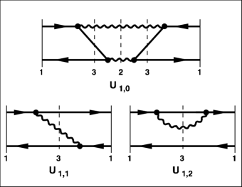
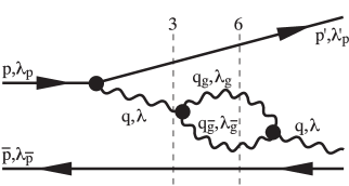
The most important result of this section is that gauge theory particularly QCD has only two structurally different contributions to the effective interaction in the $q\bar{q}$-space, see Eq.(33). The effective one-gluon exchange

$$U=VG_{3}V$$ (46)

conserves the flavor along the quark line and describes all fine and hyperfine interactions. As illustrated in Fig. 1 the vertex interaction $V$ creates a gluon and scatters the system virtually into the $q\bar{q}\,g$-space. As indicated in the figure by the vertical line with subscript ‘3’, the three particles propagate there under impact of the full Hamiltonian before the gluon is absorbed. The gluon can be absorbed either by the antiquark or by the quark. If it is absorbed by the quark, it contributes to the effective quark mass $\overline{m}$. The second term in Eq.(33), the effective two-gluon-annihilation interaction,

$$U_{a}=VG_{3}VG_{2}VG_{3}V\,,$$ (47)

is represented by the graph $U_{1,0}$ in Fig. 1. The virtual annihilation of the $q\bar{q}$-pair into two gluons can generate an interaction between different quark flavors. As a net result the effective interaction scatters a quark with helicity $\lambda_{q}$ and four-momentum $p=(xP^{+},x\vec{P}_{\!\perp}+\vec{k}_{\!\perp},p^{-})$ into a state with $\lambda_{q}^{\prime}$ and four-momentum ${p^{\prime}}=(x^{\prime}P^{+},x^{\prime}\vec{P}_{\!\perp}+\vec{k}_{\!\perp}^{\prime},{p^{\prime}}^{-})$, and correspondingly the antiquark. In the continuum limit, the resolvents are replaced by propagators and the eigenvalue problem $H_{\rm eff}|\psi\rangle=M^{2}|\psi\rangle$ becomes again an integral equation, but a very simple one in only three continuous variables ($x,\vec{k}_{\!\perp}$). Its structure is rather transparent:

$$M_{i}^{2}\langle x,\vec{k}_{\!\perp};\lambda_{q},\lambda_{\bar{q}}|\psi_{i}\rangle$$ (48)

$$=\left[{\overline{m}^{2}_{q}+\vec{k}_{\!\perp}^{2}\over x}+{\overline{m}^{2}_{\bar{q}}+\vec{k}_{\!\perp}^{2}\over 1-x}\right]\langle x,\vec{k}_{\!\perp};\lambda_{q},\lambda_{\bar{q}}|\psi_{i}\rangle$$

$$+\sum_{\lambda_{q}^{\prime},\lambda_{\bar{q}}^{\prime}}\!\int\!dx^{\prime}d^{2}\vec{k}_{\!\perp}^{\prime}\,\,\Theta(x^{\prime},k_{\perp}^{\prime})\,\langle x,\vec{k}_{\!\perp};\lambda_{q},\lambda_{\bar{q}}|VG_{3}V+$$

$$VG_{3}VG_{2}VG_{3}V|x^{\prime},\vec{k}_{\!\perp}^{\prime};\lambda_{q}^{\prime},\lambda_{\bar{q}}^{\prime}\rangle\,\langle x^{\prime},\vec{k}_{\!\perp}^{\prime};\lambda_{q}^{\prime},\lambda_{\bar{q}}^{\prime}|\psi_{i}\rangle.$$

The domain of integration is set by the sharp cut-off function $\Theta$ given in Eq.(12). The eigenvalues refer to the invariant mass $M_{i}$ of a physical state. The wavefunction $\langle x,\vec{k}_{\!\perp};\lambda_{q},\lambda_{\bar{q}}|\psi_{i}\rangle$ gives the probability amplitudes for finding in the $q\bar{q}$-state a flavored quark with momentum fraction $x$, intrinsic transverse momentum $\vec{k}_{\!\perp}$ and helicity $\lambda_{q}$, and correspondingly an anti-quark with $1-x$, $-\vec{k}_{\!\perp}$ and $\lambda_{\bar{q}}$. Both the mass and the wave-functions are boost-invariant.

5 Perturbation theory in medium

Here seems to be a problem: For calculating $G_{3}$ one needs $G_{6}$, $G_{5}$ and $G_{4}$, see Eq.(33), for calculating $G_{6}$ one needs $G_{10}$, $G_{9}$ and $G_{7}$, see Eq.(34), and so on. This property corresponds to some extent the infinite series of the Tamm-Dancoff approach, see Eq.(24). But the method of iterated resolvents resumes them systematically without double counting. In the next section will be shown how the hierarchy can be broken in a rather effective way. That final step will be comparatively simple if one has analyzed the propagators for the sectors with one $q\bar{q}$-pair and arbitrarily many gluons, as follows next.

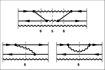
Consider first the case with one gluon as given by Eq.(34). The corresponding diagrams can be grouped into two topologically distinct classes, displayed in Figs. 2 and 3. Adding one free gluon to the diagrams in Fig. 1 produces the diagrams in Fig. 2. The gluon does not change quantum numbers under impact of the interaction and acts like a spectator. Therefore, the graphs in Fig. 2 will be referred to as the ‘spectator interaction’ $\overline{U}_{3}$. In the graphs of Fig. 3 the gluons are scattered by the interaction, and correspondingly these graphs will be referred to as the ‘participant interaction’ $\widetilde{U}_{3}$. Thus, $U_{3}=\overline{U}_{3}+\widetilde{U}_{3}$.

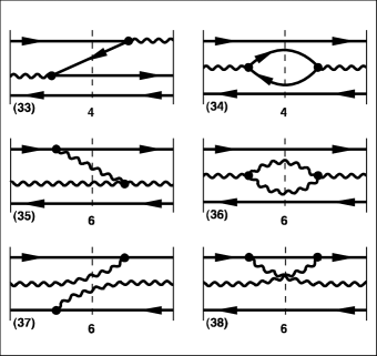
Next consider the propagator $G_{6}$ in the $q\bar{q}\,gg$-space. By drawing all possible diagrams of $U_{6}$, as given in Eq.(35), one realizes quickly that most of them topologically belong to one of the two classes which one obtains by adding a free gluon to the diagrams in Figs. 2 and  3. The effective interaction $VG_{10}V$, however, generates also an interaction between the two Fock-space gluons in $q\bar{q}\,gg$, by an effective one-gluon exchange. Potentially, these diagrams contribute to a $gg$-bound-state (a glue-ball), very much like the gluon-exchange between the quark and the antiquark contributes to a $q\bar{q}$-bound-state. By definition, these glue-ball diagrams will be included in the spectator interaction $\overline{U}_{6}$. Estimates on their size will be given elsewhere pau98 .

The separation into spectators and participants can be made in all quark-pair-gluon sector interactions:

$$U_{n}=\overline{U}_{n}+\widetilde{U}_{n}\ ,\quad{\rm for}\quad n=3,6,10,15,\dots\ .$$ (49)

More explicitly, the spectator interactions in the lowest sectors with one quark-pair become for example

$$\overline{U}_{3} = VG_{6}V\ +VG_{6}VG_{5}VG_{6}V\,,$$ (50)

$$\overline{U}_{6} = VG_{10}V+VG_{10}VG_{9}VG_{10}V\,.$$ (51)

Correspondingly the participant interactions are

$$\widetilde{U}_{3} = VG_{4}V\ +VG_{6}V\,,$$ (52)

$$\widetilde{U}_{6} = VG_{7}V\ +VG_{10}V\,.$$ (53)

The same operators appear in both $\overline{U}$ and $\widetilde{U}$.

Since the Hamiltonian is additive in spectator and participant interactions, $\overline{U}_{n}$ can be associated with

$$\overline{G}_{n}={1\over\omega-T_{n}-\overline{U}_{n}}\,,$$ (54)

$$\biggl{(}{\rm while\ }G_{n}\equiv{1\over\omega-H_{n}}={1\over\omega-T_{n}-\overline{U}_{n}-\widetilde{U}_{n}}\ \biggr{)}\,.$$

The relation to the full resolvent $G_{n}=\overline{G}_{n}+\overline{G}_{n}\,\widetilde{U}_{n}\,G_{n}$ is exact. Equivalently, it is written as an infinite series

$$G_{n}=\overline{G}_{n}+\overline{G}_{n}\widetilde{U}_{n}\,\overline{G}_{n}+\overline{G}_{n}\widetilde{U}_{n}\,\overline{G}_{n}\widetilde{U}_{n}\,\overline{G}_{n}+\dots\,.$$ (55)

The difference to the perturbative Tamm-Dancoff series is that the ‘unperturbed propagator’ $G_{0}(\omega)$ in Eq.(24) refers to the system without interactions while here the ‘unperturbed propagator’ $\overline{G}_{n}$ contains the interaction in the well defined form of $\overline{U}_{n}$. One deals here with a perturbation theory in medium.

Figure 2: The three graphs of the spectator interaction in the $q\bar{q}\,g$-space. Note the role of the gluon as a spectator.

The different physics should be emphasized: The system is not scattered into other sectors, it stays in sector $n$. This is reflected in an operator identity,

$$(\omega-\overline{H}_{n})(1-\widetilde{U}_{n}\overline{G}_{n})=\omega-H_{n},$$ (56)

which is obtained straightforwardly from Eqs.(49) and (54). The inverse gives $R_{n}^{2}\,\overline{G}_{n}=G_{n}$, with

$$R_{n}=\sqrt{{1\over 1-\overline{G}_{n}\widetilde{U}_{n}}}\,.$$ (57)

With the obvious identity $R_{n}\,\overline{G}_{n}=\overline{G}_{n}\,R_{n}^{\dagger}$, one ends up with $G_{n}=R_{n}\,\overline{G}_{n}\,R_{n}^{\dagger}$. In all of the above effective interactions the $R_{n}$ are sandwiched between a quark-pair-glue resolvent $\overline{G}$ and the vertex $V$,

$$V\,G_{n}\,V^{\dagger}=V\,R_{n}\,\overline{G}_{n}\,R_{n}^{\dagger}\,V^{\dagger}=\overline{V}\,\overline{G}_{n}\,\overline{V}^{\dagger}\,.$$ (58)

Each block matrix $V$ is rectangular and multiplied with a square matrix $R_{n}$ according to

$$\overline{V}=VR_{n},\qquad{\rm or}\qquad\overline{V}^{\dagger}=R_{n}^{\dagger}V^{\dagger}\,.$$ (59)

In the sequel we shall suppress again the dagger indicating the hermitean conjugate matrix. In Section 7 will be shown that $R_{n}$ is essentially diagonal and independent of the spin, such that each vertex matrix element is multiplied with a number, actually with a number which depends on the momentum transfer $Q$ across the vertex. Equivalently one replaces the coupling constant $g$ by an effective coupling constant $\overline{g}$, i.e.

$$g\longrightarrow\overline{g}(Q)=gR_{n}(Q)\,.$$ (60)

$R_{n}$ has thus the interpretation of a vertex function.

One can thus rewrite Eqs.(33), (50) and (51) in such a form that they are all essentially equal, i.e.

$$\overline{U}_{6} = \overline{V}\,\overline{G}_{10}\overline{V}+\overline{V}\,\overline{G}_{10}\overline{V}G_{9}\overline{V}\,\overline{G}_{10}\overline{V}\ ,$$ (61)

$$\overline{U}_{3} = \overline{V}\,\overline{G}_{6}\overline{V}+\overline{V}\,\overline{G}_{6}\overline{V}G_{5}\overline{V}\,\overline{G}_{6}\overline{V}\ ,$$ (62)

$$U_{1} = \overline{V}\,\overline{G}_{3}\overline{V}+\overline{V}\,\overline{G}_{3}\overline{V}G_{2}\overline{V}\,\overline{G}_{3}\overline{V}\,.$$ (63)

The effective sector Hamiltonians $\overline{H}_{n}=T_{n}+\overline{U}_{n}$ describes bound states of one $q\bar{q}$-pair with arbitrarily many gluons and glue balls. Approximatively, one can relate them to each other, see Sec. 6.

Figure 3: Some six graphs of the participant interaction in the $q\bar{q}\,g$-space.

The content of Sects. 4 and 5 is exact but rather formal. To show its usefulness, rigor will be given up in the sequel in favor of transparency and the aim to obtain a simple and solvable equation. It should be emphasized here already that the content of Sects. 6 and 7 will have to be substantiated in future work pau98 .

6 The breaking of the propagator hierarchy

All effective sector Hamiltonians can be diagonalized on their own merit. To shape notation, the first few eigenvalue equations are written down explicitly. In the $q\bar{q}$-space they read in Fock space representation

$$M_{1;i}^{2}\,\langle q;\bar{q}|\psi_{i}^{(1)}\rangle=\sum_{q^{\prime},\bar{q}^{\prime}}\langle q;\bar{q}|H_{1}|q^{\prime};\bar{q}^{\prime}\rangle\,\langle q^{\prime};\bar{q}^{\prime}|\psi_{i}^{(1)}\rangle.$$ (64)

For simplicity, the eigenvalues are enumerated by $i=0,1,2,\dots,\infty$. In the sequel, the lowest eigenvalue is supposed to satisfy the fix-point equation $\omega=M^{2}_{1,0}(\omega)$ and its numerical value will be denoted by $M^{2}$. Correspondingly, one has in the $gg$-space

$$M_{2;j}^{2}\,\langle g;\bar{g}|\psi_{j}^{(2)}\rangle=\sum_{g^{\prime},\bar{g}^{\prime}}\langle g;\bar{g}|H_{2}|g^{\prime};\bar{g}^{\prime}\rangle\,\langle g^{\prime};\bar{g}^{\prime}|\psi_{j}^{(2)}\rangle,$$ (65)

and in the $q\bar{q}\,g$ space

$$\overline{M}_{3;j}^{2}\,\langle q;\bar{q};g|\psi_{j}^{(3)}\rangle$$ (66)

$$=\sum_{q^{\prime},\bar{q}^{\prime},g^{\prime}}\langle q;\bar{q};g|\overline{H}_{3}|q^{\prime};\bar{q}^{\prime};g^{\prime}\rangle\,\langle q^{\prime};\bar{q}^{\prime};g^{\prime}|\psi_{j}^{(3)}\rangle.$$

Knowing the complete sets of eigenfunctions, one can calculate the exact resolvents in Fock space representation, as for example the resolvent in the two gluon sector

$$\langle g;\bar{g}|G_{2}(\omega)|g^{\prime};\bar{g}^{\prime}\rangle$$ (67)

$$=\sum_{j}\langle g;\bar{g}|\psi_{j}^{(2)}\rangle{1\over\omega-M_{2;j}^{2}}\langle\psi_{j}^{(2)}|g^{\prime};\bar{g}^{\prime}\rangle.$$

As often in many-body physics, one approximates resolvents by assuming that all eigenvalues are degenerate with the lowest state, which here is the glue ball mass $M^{2}_{g}$. One then applies closure

$$\langle g;\bar{g}|G_{2}|g^{\prime};\bar{g}^{\prime}\rangle={1\over M^{2}-M_{g}^{2}}\sum_{j}\langle g;\bar{g}|\psi_{j}\rangle\langle\psi_{j}|g^{\prime};\bar{g}^{\prime}\rangle$$ (68)

in order to obtain a diagonal resolvent

$$\langle g;\bar{g}|G_{2}|g^{\prime};\bar{g}^{\prime}\rangle={1\over M^{2}-M_{g}^{2}}\langle g;\bar{g}|g^{\prime};\bar{g}^{\prime}\rangle.$$ (69)

The propagator in the $q\bar{q}g$-space could be calculated by the same procedure, but one can do better. Since the gluon is a free particle which moves relative to the $q\bar{q}$-bound state, the eigenfunction $|\psi_{j}^{(3)}\rangle=|\psi_{i}^{(1)}\rangle\otimes|\varphi_{s}\rangle$ is a product state. The $q\bar{q}g$-eigenvalues

$$\overline{M}_{3;j}^{2}\equiv\overline{M}_{3;i,s}^{2}={M_{1;i}^{2}+\vec{q}_{\!\perp}^{\,2}\over(1-y)}+{\vec{q}_{\!\perp}^{\,2}\over y}\,,$$ (70)

can therefore be expressed in terms of the $q\bar{q}$-eigenvalues. Every $q\bar{q}$-bound state is band head for a continuum of gluons. With the four-momenta $q^{\mu}=(yP^{+},y\vec{P}_{\!\perp}+\vec{q}_{\!\perp},q_{g}^{-})$ one gets for the lowest bound state

$$\omega-\overline{M}_{3;0,s}^{2}\equiv M^{2}-\overline{M}_{3;0,s}^{2}=-{y^{2}M^{2}+\vec{q}_{\!\perp}^{\,2}\over y(1-y)}\,.$$ (71)

Assuming a degenerate spectrum and performing closure,

$$\langle q;\bar{q};g|\overline{G}_{3}|q^{\prime};\bar{q}^{\prime};g^{\prime}\rangle=\overline{G}_{3}(q;\bar{q};g)\langle q;\bar{q};g|q^{\prime};\bar{q}^{\prime};g^{\prime}\rangle,$$ (72)

one gets the delta function $\langle q;\bar{q};g|q^{\prime};\bar{q}^{\prime};g^{\prime}\rangle$ multipied with

$$\overline{G}_{3}(q;\bar{q};g)=-{y\over Q^{2}},\ Q^{2}=(y^{2}M^{2}+\vec{q}_{\!\perp}^{\,2}){1\over 1-y}.$$ (73)

Note that Eqs.(69) and (73) break the hierarchy of the iterated resolvents. For calculating the effective interaction in the $q\bar{q}$-space only the two resolvents $\overline{G}_{3}$ and $G_{2}$ are needed. Both are written now in closed expressions. The whole complication of having resolvents of resolvents is replaced by the problem of knowing the eigenvalues $M$ and $M_{g}$ ahead of time. Good initial guesses ($M_{0}$) might suffice but can be improved iteratively with $M_{n}\rightarrow M_{n+1}$.

The notation in Eq.(73) is suggestive for $Q^{2}$ being related to the single-particle four-momentum transfer along the quark line. The free propagator in the $q\bar{q}g$-space can be written bpp97

$$G_{q\bar{q}g,{\rm free}} = {1\over P^{+}(p^{-}-p^{\prime-}-q^{-})}={y\over(p-p^{\prime})^{2}}\,.$$ (74)

The single-particle notation refers to Fig. 4. For sufficiently small $y$ holds $(p-p^{\prime})^{2}=-[y^{2}(2\overline{m})^{2}+\vec{q}_{\!\perp}^{\,2}]$. If one substitutes $M\simeq 2\overline{m}$, which holds to rather good approximation, the momentum transfer in Eq.(74) is the same as in Eq.(73). One concludes: In the solution, the interacting particles propagate like free particles to a high degree of approximation; they just acquire an effective mass.

Most importantly, instead of having resolvents of resolvents, the hierarchy of iterated resolvents is broken. Ex post, this justifies the $\omega=\omega^{\star}$ trick in the Tamm-Dancoff work kpw92 ; trp96 .

One can restore the exact $q\bar{q}g$-propagator by addition and subtraction, which gives

$$\langle q;\bar{q};g|\overline{G}_{3}|q^{\prime};\bar{q}^{\prime};g^{\prime}\rangle=\overline{G}_{3}(q;\bar{q};g)$$ (75)

$$\times\left[\langle q;\bar{q};g|q^{\prime};\bar{q}^{\prime};g^{\prime}\rangle-\langle q;\bar{q};g|A|q^{\prime};\bar{q}^{\prime};g^{\prime}\rangle\right].$$

In Eq.(72) the operator $A$ was neglected, with

$$A=\sum_{i,s}|\psi_{i,s}^{(3)}\rangle\,{y(M_{1;i}^{2}-M^{2})\over Q^{2}+y(M_{1;i}^{2}-M^{2})}\,\langle\psi_{i,s}^{(3)}|\,.$$ (76)

Probably, this is the most drastic assumption in this work. It suppresses the appearance of the Lamb-shift.

Note that the above approximations can be controlled e posteriori: Once the eigenfunctions in the $q\bar{q}$-sector are available numerically, one can check whether the exact definition of the resolvent Eq.(72) is peaked like a $\delta$-function, with a residue predicted by Eq.(73).

7 Perturbative analysis of the vortices

Having established that the propagator $\overline{G}_{3}$ can be approximated by the free propagator, one can calculate the vertex function $R_{3}$ straightforwardly. According to Eq.(57) one has

$$R_{3}=\sqrt{{1\over 1-\overline{G}_{3}\widetilde{U}_{3}}}=1+{1\over 2}\overline{G}_{3}\widetilde{U}_{3}+{3\over 8}\overline{G}_{3}\widetilde{U}_{3}\,\overline{G}_{3}\widetilde{U}_{3}+\dots\,.$$ (77)

It is reasonable to restrict to the first non-trivial term in the expansion

$$\overline{V}=VR_{3}\simeq V+{1\over 2}\left(V\overline{G}_{3}V\overline{G}_{4}V+V\overline{G}_{3}V\overline{G}_{6}V\right)\,.$$ (78)

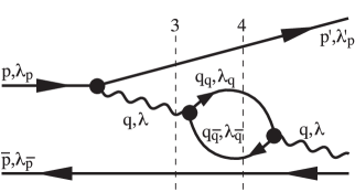
Since the contributions from the vertex functions $R_{4}$ and $R_{6}$ generate terms of higher orders in $g$, one must set $R_{4}=R_{6}=1$, in order to be consistent. A diagrammatic analysis of Eq.(78) un-reveals quickly that it is the familiar ‘vertex correction’, which has been calculated in the front form by Thorn tho79 and by Perry phz93 . Thorn and later Perry, however, were motivated primarily by asymptotic freedom ‘on the light-cone’ and thus have emphasized the behaviour at large momentum transfer $Q\rightarrow\infty$. In the present context one is interested in the opposite limit $Q\rightarrow 0$. In a bound state equation such as Eq.(48) the region near the Coulomb singularity $Q\sim 0$ is very important. Raufeisen rap97 has recalculated therefore all about 22 diagrams of the vertex correction in light-cone perturbation theory, see for example bpp97 . The salient features of these calculations will be exposed here at hand of the two vacuum polarization diagrams in Figs. 4 and 5.

Figure 4: The $q\bar{q}$ vacuum polarization graph.

Next let us calculate the free propagator in the $q\bar{q}\,q\bar{q}$-sector, i.e.

$$\overline{G}_{4}={1\over({p}^{-}-{p^{\prime}}^{-}-q_{q}^{-}-\bar{q}_{\bar{q}}^{-})P^{+}}.$$ (79)

Parameterizing in Fig. 4 the intermediate particle momenta as

$$q_{q}^{\mu}=\left(yzP^{+},yz\vec{P}_{\!\perp}+z\vec{q}_{\!\perp}+\vec{l}_{\!\perp},q_{q}^{-}\right),\bar{q}_{\bar{q}}^{\mu}=$$

$$\left(y(1-z)P^{+},y(1-z)\vec{P}_{\!\perp}+(1-z)\vec{q}_{\!\perp}-\vec{l}_{\!\perp},\bar{q}_{\bar{q}}^{-}\right),$$ (80)

and using the four-momentum transfer along the quark line $Q$ as defined in Eq.(73) the propagator becomes

$$\overline{G}_{4}=-{q_{g}^{+}\over P^{+}}{z(1-z)\over z(1-z)Q^{2}+\vec{l}_{\!\perp}^{\,2}+m^{2}_{f}}.$$ (81)

Evaluating the spinor summations gives for $n_{f}$ flavors

$$V\overline{G}_{3}V\overline{G}_{4}V=-V\sum_{f=1}^{n_{f}}{\alpha\over 4\pi}\int\!dz\,dl_{\perp}^{2}$$ (82)

$$\Theta(z,l_{\perp}){1-2z(1-z)-\bigg{[}{2m_{f}^{2}\over Q^{2}}\bigg{]}\over l_{\perp}^{2}+m_{f}^{2}+z(1-z)Q^{2}}.$$

Note the spin-independent factor to the matrix element $V$. The cut-off function $\Theta$ was defined in Eq.(12). The term in the square brackets are cancelled by other diagrams and will be disregarded in the sequel. Integrating over $l_{\perp}$ yields straightforwardly

$$\overline{G}_{3}V\overline{G}_{4}V=-\sum_{f}{\alpha\over 4\pi}$$ (83)

$$\int\limits_{\epsilon_{f}}^{1-\epsilon_{f}}\!\!\!dz\,\bigg{(}1-2z(1-z)\bigg{)}\ \ln{{\Lambda^{2}+4m_{f}^{2}+Q^{2}\over Q^{2}+{m_{f}^{2}\over z(1-z)}}}\,.$$

The integral over $z$ is non-trivial. Since the logarithm is a very weak function of its arguments, the term $m_{f}^{2}/z(1-z)$ is replaced by its maximum at $z={1\over 2}$, thus

$$\overline{G}_{3}V\overline{G}_{4}V=-\sum_{f}{\alpha\over 6\pi}\ln{\bigg{(}1+{\Lambda^{2}\over 4m_{f}^{2}+Q^{2}}\bigg{)}}\,.$$ (84)

The corresponding steps for the propagator in the $q\bar{q}\,gg$-sector (Fig. 5) give with $\overline{G}_{6}=\big{[}({p}^{-}-{p^{\prime}}^{-}-q_{g}^{-}-\bar{q}_{g}^{-})P^{+}\big{]}^{-1}$

$$\overline{G}_{6}=-{q_{g}^{+}\over P^{+}}{z(1-z)\over z(1-z)Q^{2}+\vec{l}_{\!\perp}^{\,2}+m^{2}_{g}}.$$ (85)

For the purpose of regularization the gluon is endorsed with a small regulator mass $m_{g}$, see Sec. 2.

Figure 5: The $gg$ vacuum polarization graph.

The spinor sums yield

$$V\overline{G}_{3}V\overline{G}_{6}V=V\,{\alpha n_{c}\over 2\pi}\int\!dz\,dl_{\perp}^{2}$$ (86)

$$\Theta(z,l_{\!\perp})\,{2-z(1-z)\,-\bigg{[}{1\over z(1-z)}\bigg{]}\over l_{\perp}^{2}+m^{2}_{g}+z(1-z)Q^{2}}\,.$$

Dropping the term in the square bracket, and performing the same approximation as above gives

$$\overline{G}_{3}V\overline{G}_{6}V={11\alpha n_{c}\over 12\pi}\ln{\bigg{(}1+{\Lambda^{2}\over 4m^{2}_{g}+Q^{2}}\bigg{)}}\,.$$ (87)

As a net result, the coupling constant $g$ has to be replaced by the effective coupling constant $\overline{g}$, i.e. $g\rightarrow\overline{g}$ with

$$\overline{g}=gR_{3}=g\left(1+{1\over 2}\alpha b(Q)\right)\,,$$ (88)

see also rap97 . The function $b(Q)$ depends on the momentum transfer (and on the cutoff), i.e.

$$b(Q)={11n_{c}\over 12\pi}\ln{\bigg{(}1+{\Lambda^{2}\over 4m^{2}_{g}+Q^{2}}\bigg{)}}-$$ (89)

$${1\over 6\pi}\sum_{f}\ln{\bigg{(}1+{\Lambda^{2}\over 4m_{f}^{2}+Q^{2}}\bigg{)}}\,$$

and generates therefore a new interaction. Finally, the effective quark masses become according to the diagram $U_{1,2}$ in Fig. 1

$$\overline{m}_{f}^{2}=m_{f}^{2}+m_{f}^{2}{\alpha\over\pi}{n_{c}^{2}-1\over 2n_{c}}\ln{{\Lambda^{2}\over m_{g}^{2}}}\,.$$ (90)

A similar diagram for the effective gluon mass gives

$$\overline{m}_{g}^{2}=m^{2}_{g}-{\alpha\over 4\pi}\sum_{f}m_{f}^{2}\ \ln{\bigg{(}1+{\Lambda^{2}\over 4m_{f}^{2}}\bigg{)}}\,.$$ (91)

Both are obtained by light-cone perturbation theory bpp97 combined with vertex regularization.

The above considerations are perturbative, as mentioned. What happens if one substitutes the free propagators in Eqs.(81) and (85) by the non-perturbative propagators $\overline{G}_{4}=(\omega-\overline{H}_{q\bar{q}\,q\bar{q}})^{-1}$ and $\overline{G}_{6}=(\omega-\overline{H}_{q\bar{q}\,gg})^{-1}$, at least in an approximate fashion? — There are additional graphs. In the fermion loop of vacuum polarization appear two graphs in addition to Fig. 4. In one of them, a gluon is emitted and absorbed on the same quark line which changes the bare quark mass $m_{f}$ into the physical quark mass $\overline{m}_{f}$. In the other graph, the gluon is emitted from the quark and absorbed by the anti-quark which represents an interaction. In consequence one has a bound state with a physical mass scale $\mu_{f}$. We replace therefore

$$2m_{f}\Longrightarrow 2\overline{m}_{f}\Longrightarrow\mu_{f}.$$ (92)

Similar considerations hold for the gluon loop in Fig. 5 and lead to the substitution

$$2m_{g}\Longrightarrow 2\overline{m}_{g}\Longrightarrow\mu_{g}.$$ (93)

Both $\mu_{g}$ and $\mu_{f}$ are interpreted as physical mass scales. The physical gluon mass $\overline{m}_{g}$ vanishes of course due to gauge invariance. This is not in conflict with f.e. Cornwall’s suggestion of a finite effective gluon mass cor83 since one can define $(\overline{m}_{g})_{\rm eff}\equiv\mu_{g}/2$. Estimates are given in Eq.(103), and discussed in Sec. 9. In conclusion, for sufficiently large $\Lambda$, one replaces Eq.(89) by

$$b(Q)={11n_{c}\over 12\pi}\ln{\bigg{(}{\Lambda^{2}\over\mu^{2}_{g}+Q^{2}}\bigg{)}}-{1\over 6\pi}\sum_{f}\ln{\bigg{(}{\Lambda^{2}\over\mu_{f}^{2}+Q^{2}}\bigg{)}}.$$ (94)

For $Q\gg(\mu_{g},\mu_{f})$ this becomes

$$b(Q)=b_{0}\ln{\bigg{(}{\Lambda^{2}\over Q^{2}}\bigg{)}},\quad{\rm with}\qquad b_{0}={33-2n_{f}\over 12\pi},$$ (95)

for $n_{c}=3$. It coincides with the perturbative expressions of Thorn and of Perry. The notation is inspired by the relation to the familiar beta-function wei95 .

8 Renormalization

Now, all the pieces are together which are needed for a further discussion of the effective interaction as defined in Eq.(48). In the present first assault the flavor changing interaction $U_{a}$ is disregarded. In the remainder $U$, the instantaneous interaction is restored by $\overline{U}_{q\bar{q}}=W_{q\bar{q}}+\overline{V}\,\overline{G}_{q\bar{q}\,g}\overline{V}$, with $\overline{G}_{q\bar{q}\,g}$ given by Eq.(73). Both terms contain a non-integrable singularity which however cancel each other such that only the integrable Coulomb singularity $Q^{-2}$ remains, see for example bpp97 . When substituting in both of them $g\rightarrow\overline{g}$ one gets from Eq.(48) the final one-body equation:

$$M^{2}\langle x,\vec{k}_{\!\perp};\lambda_{q},\lambda_{\bar{q}}|\psi\rangle=$$ (96)

$$\left[{\overline{m}^{\,2}_{q}+\vec{k}_{\!\perp}^{\,2}\over x}+{\overline{m}^{\,2}_{\bar{q}}+\vec{k}_{\!\perp}^{\,2}\over 1-x}\right]\langle x,\vec{k}_{\!\perp};\lambda_{q},\lambda_{\bar{q}}|\psi\rangle$$

$$-{1\over 3\pi^{2}}\sum_{\lambda_{q}^{\prime},\lambda_{\bar{q}}^{\prime}}\!\int\!dx^{\prime}d^{2}\vec{k}_{\!\perp}^{\prime}\,\Theta(x^{\prime},k_{\perp}^{\prime})$$

$${\overline{\alpha}(Q)\over Q^{2}}\,\langle\lambda_{q},\lambda_{\bar{q}}|S(Q)|\lambda_{q}^{\prime},\lambda_{\bar{q}}^{\prime}\rangle\,\langle x^{\prime},\vec{k}_{\!\perp}^{\prime};\lambda_{q}^{\prime},\lambda_{\bar{q}}^{\prime}|\psi\rangle.$$

The effective coupling constant $\overline{\alpha}(Q)=\overline{g}^{2}(Q)/4\pi$ has thus far been given in Eq.(88); its renormalized version will be given in Eq.(108), below. The cut-off function $\Theta$ sets the domain of integration and was defined in Eq.(12). The spinor factor $S(Q)$ represents the familiar current-current coupling which describes all fine and hyperfine interactions

$$\langle\lambda_{q},\lambda_{\bar{q}}|S(Q)|\lambda_{q}^{\prime},\lambda_{\bar{q}}^{\prime}\rangle=$$ (97)

$${\left[\overline{u}(k_{q},\lambda_{q})\gamma^{\mu}u(k_{q}^{\prime},\lambda_{q}^{\prime})\right]\over\sqrt{xx^{\prime}}}\,{\left[\overline{u}(k_{\bar{q}},\lambda_{\bar{q}})\gamma_{\mu}u(k_{\bar{q}}^{\prime},\lambda_{\bar{q}}^{\prime})\right]\over\sqrt{(1-x)(1-x^{\prime})}}.$$

Actually, the precise analysis of the formalism requires to use the arithmetic mean from each vertex, i.e.

$${\overline{\alpha}(Q)\over Q^{2}}\Longrightarrow{1\over 2}\sqrt{\overline{\alpha}(Q_{q})\overline{\alpha}(Q_{\bar{q}})}\left({1\over Q_{q}^{2}}+{1\over Q_{\bar{q}}^{2}}\right)\,,$$ (98)

where $Q^{2}_{q}=-(p_{q}-p_{q}^{\prime})^{2}$ and $Q^{2}_{\bar{q}}=-(p_{\bar{q}}-p_{\bar{q}}^{\prime})^{2}$ are the momentum transfers along the quark and the antiquark line, respectively. Close to the Coulomb singularity, however, this does not matter since both are approximately equal: $Q^{2}_{q}\simeq Q^{2}_{\bar{q}}\simeq(m_{q}+m_{\bar{q}})^{2}(x-x^{\prime})^{2}+(\vec{k}_{\!\perp}-\vec{k}_{\!\perp}^{\prime})^{2}$.

Let us return to Eq.(88). The analysis there was incomplete and limited to the lowest perturbative order rather than to resume the series to all orders in $\alpha$ as required by the definition of the vertex function, Eq.(77). One can calculate the second order diagram if one neglects all genuine two-loop contributions. More generally, if one neglects all $n$-loop contributions one can calculate the term of $n$-th order by

$$\left(\overline{G}_{3}V\overline{G}_{4}V+\overline{G}_{3}V\overline{G}_{6}V\right)^{n}\simeq\left(\alpha b(Q)\right)^{n},$$ (99)

and resume the series formally to all orders, i.e.

$$\overline{g}(Q)={g\over\sqrt{1-\alpha b(Q)}},\ {\rm thus}\quad\overline{\alpha}(Q)={\alpha\over 1-\alpha b(Q)}.$$ (100)

The restriction to the one-loop level is a customary procedure and not coupled directly to the size of $\alpha$. More important is the point that the series converges only if

$$\alpha b(Q)\leq 1\,,$$ (101)

for all $Q$ and $\alpha$. Let us therefore discuss shortly to which extent Eq.(101) holds true. The possibility of $\alpha\ll 1$ is disregarded, since considerations should not be limited by perturbative considerations. According to Eq.(94), $b(Q)$ is largest for $Q=0$. Defining a weighted average $\mu$ by

$$b_{0}\ln{\bigg{(}{\Lambda^{2}\over\mu^{2}}\bigg{)}}\equiv{33\over 12\pi}\ln{\bigg{(}{\Lambda^{2}\over\mu^{2}_{g}}\bigg{)}}-{1\over 6\pi}\sum_{f}\ln{\bigg{(}{\Lambda^{2}\over\mu_{f}^{2}}\bigg{)}},$$ (102)

gives $\mu^{2}\geq\Lambda^{2}e^{-{1\over\alpha b_{0}}}$ from Eq.(101). This lower limit is not necessarily small. An estimate appropriate for charmonium ($M_{c}$) (with $\Lambda\simeq M_{c}$ and $\alpha b_{0}\sim 0.2$) rather gives $\mu\geq 245{\,\rm MeV}$. Denote the six experimental masses for the neutral scalar mesons with $M_{f}$ and the estimated glue-ball mass with $M_{g}\sim 1.4$ GeV. The scales $\mu_{f}$ and $\mu_{g}$ are identified with them for simplicity. One gets from Eq.(102)

$$\mu_{g}=M_{g},\ \mu_{f}=M_{f},\quad{\rm thus}\quad\mu=0.91\ {\rm GeV},$$ (103)

independent of $\Lambda$ and consistent with the above limit.

This is as far as one can go with the regulated theory. Next let us address to the renormalization of the theory, particularly to the renormalization group equations. The eigenvalues of the light-cone Hamiltonian $H_{LC}$ are given by Eq.(96). Potentially, they depend on $\Lambda$ through three sources: (1) the physical flavor masses $\overline{m}_{f}$; (2) the $\Theta$-function representing the domain of integration; (3) the effective coupling constant $\overline{\alpha}(Q)$. Only the last one is relevant, since the flavor masses are renormalization group invariants with $d\overline{m}_{f}/d\Lambda=0$, and since (at least in a confining regime) the wavefunctions decay sufficiently fast to serve as a natural cut-off. It is thus reasonable to replace Eq.(7) by

$${d\over d\Lambda}\,\overline{\alpha}(\alpha;\Lambda)=0\,.$$ (104)

It can be satisfied by a cut-off dependent bare coupling constant $g=g(\Lambda)$, thus by

$${d\overline{\alpha}\over d\Lambda}={1\over\displaystyle\left(1-\alpha b(Q)\right)^{2}}\left({d\alpha\over d\Lambda}+\alpha^{2}{db\over d\Lambda}\right)=0\,.$$ (105)

Since $db/d\Lambda$ is completely independent of the mass scales $\mu_{g}$ and $\mu_{f}$ appearing in Eq.(94), i.e.

$${db(Q)\over d\Lambda}=2{b_{0}\over\Lambda}\,,$$ (106)

one gets the differential equation ${d\alpha/d\Lambda}=-2\alpha^{2}b_{0}/\Lambda$, as usual, including its solution wei95

$$\alpha_{\Lambda}={\alpha_{0}\over 1+\alpha_{0}b_{0}\ln{{\Lambda^{2}\over\Lambda^{2}_{0}}}}={1\over b_{0}\ln{{\Lambda^{2}\over\Lambda_{QCD}^{2}}}}\,.$$ (107)

The renormalization point $\alpha_{0}$ at the scale $\Lambda_{0}$ is arbitrary. The two parameters $(\alpha_{0},\Lambda_{0})$ can therefore be compounded into a single one, into the QCD-scale $\Lambda_{QCD}\equiv\kappa$ which is defined by $2\alpha_{0}b_{0}\ln{\Lambda_{0}/\Lambda_{QCD}}=1$. Substituting Eq.(107) back into into Eq.(100) gives

$$\overline{\alpha}(Q)={1\over\displaystyle b_{0}\ln{{\Lambda^{2}\over\displaystyle\kappa^{2}}}\bigg{(}1-{b(Q)\over\displaystyle b_{0}\ln{{\Lambda^{2}\over\displaystyle\kappa^{2}}}}\bigg{)}}={1\over\displaystyle b_{0}\ln{{\Lambda^{2}\over\displaystyle\kappa^{2}}}-b(Q)},$$

and thus

$$\overline{\alpha}(Q)={12\pi\over\displaystyle 33\ln{\bigg{(}{\mu^{2}_{g}+Q^{2}\over\kappa^{2}}\bigg{)}}-2\sum_{f}\ln{\bigg{(}{\mu^{2}_{f}+Q^{2}\over\kappa^{2}}\bigg{)}}},$$ (108)

All $\ln{(\Lambda)}$ terms cancel exactly without smallness assumption. The cancelation is directly related to the minus sign in Eq.(100), which in turn is related to the re-summation of the series to all orders in $\alpha$. Using Eq.(88), the cancelation would hold only perturbatively, for sufficiently small $\alpha$.

Since $\overline{\alpha}$ becomes independent of $\Lambda$, one can go to the limit $\Lambda\rightarrow\infty$. In line with the modern interpretation of the renormalization group one can integrate Eq.(96) unrestrictedly over all $Q$. Note the subtle difference between the ‘running coupling constant’ $g_{\Lambda}$ and the ‘effective coupling constant’ $\overline{g}(Q)$. The two are confused often in the literature. The Lagrangian does not know about the momentum transfer.

A final word on the complete wavefunction $|\Psi\rangle$. The solutions of the integral equation Eq.(96) represent the normalized projections of the full eigenfunction $|\Psi\rangle$ onto the Fock states $|q;\bar{q}\rangle=b^{\dagger}_{q}d^{\dagger}_{\bar{q}}|vac\rangle$, i.e. $\psi^{(1)}=\langle 1|\Psi\rangle$. Unlike in other methods this knowledge is sufficient in the present method to retrieve all other Fock-space components $\langle n|\Psi\rangle$ without solving another eigenvalue problem. As an example, let us work that out explicitly, by asking for the probability amplitude to find a $|gg\rangle$- and a $|q\bar{q}\,g\rangle$-state in a full eigenstate $|\Psi\rangle$.

The key is the upwards recursion relation Eq.(26). The first two equations of the recursive set in Eq.(26) are

$$\langle 2|\Psi\rangle = G_{2}\langle 2|H_{2}|1\rangle\langle 1|\Psi\rangle,$$ (109)

$$\langle 3|\Psi\rangle = G_{3}\langle 3|H_{3}|1\rangle\langle 1|\Psi\rangle+G_{3}\langle 3|H_{3}|2\rangle\langle 2|\Psi\rangle\,.$$ (110)

The sector Hamiltonians $H_{n}$ have to be substituted from Eqs.(34) and (42). In taking block matrix elements of them, the formal expressions are simplified considerably since many of the Hamiltonian blocks in Table 1 are zero. One thus gets simply $\langle 2|H_{2}|1\rangle=\langle 2|VG_{3}V|1\rangle$ and therefore $\langle 2|\Psi\rangle=G_{2}VG_{3}V\langle 1|\Psi\rangle$. Substituted into Eq.(109) this gives $\langle 3|\Psi\rangle=G_{3}V\langle 1|\Psi\rangle+G_{3}VG_{2}VG_{3}V\langle 1|\Psi\rangle$. These findings are summarized more readable

$$\langle gg|\Psi\rangle=\langle gg|G_{gg}VG_{q\bar{q}\,g}V\>|\psi_{q\bar{q}}\rangle,$$ (112)

$$\langle q\bar{q}\,g|\Psi\rangle=\langle q\bar{q}\,g|G_{q\bar{q}\,g}V\>|\psi_{q\bar{q}}\rangle$$

$$+\langle q\bar{q}\,g|G_{q\bar{q}\,g}VG_{gg}VG_{q\bar{q}\,g}V\>|\psi_{q\bar{q}}\rangle.$$

Correspondingly, one is able to find the Fock-space amplitude in the higher sectors with remarkably little effort. Of course, one has to readjust the overall normalization of the wavefunction. It should be emphasized that the finite number of terms is in strong contrast to the infinite perturbative series. Iterated resolvents resume the series to all orders in closed form. It also should be emphasized that the same approximations as discussed above must be made for reasons of consistency, particularly the effective coupling constant $\overline{g}(Q)$ must be used.

9 Summary and discussion

The present work is based on Lagrangian gauge field theory for SU(N) and on its canonical front-form Hamiltonian in the light-cone gauge $A^{+}=0$. The notational background is laid down in Sects. 2 and 3. All zero modes are disregarded, and in consequence the vacuum is trivial. Imposing periodic boundary conditions the Hamiltonian is converted to a matrix. The matrix is finite by means of Fock-space regularization. All possible divergences are controlled by vertex regularization. Being confronted with the diagonalization of a finite but large matrix, the problem is mapped on a smaller space as was done first by Tamm and by Dancoff in their theory of effective interactions. Binding effects arise then due to virtual scattering into higher Fock-space sectors. The apparent difficulties with this approach are related to the infinite perturbative series one is forced to work with in practice. A re-analysis shows that the main idea can be maintained if one introduces a hierarchy of effective interactions, in each sector of the Hilbert space. The result is an iterative procedure, called the method of iterated resolvents. Each resolvent is the inverse of an effective sector Hamiltonian which in turn is a functional of resolvents in higher sectors. For the model case of a finite matrix (DLCQ) the method of iterated resolvents can be realized and explicitly checked by a finite number of successive matrix inversions and multiplications. But even for the continuum it is a well defined and exact procedure. The infinite perturbative series of the Tamm-Dancoff approach and all their many-body aspects are then replaced by a finite number of terms. The effective interaction between a quark and an antiquark turns out to have only two contributions: The flavor conserving interaction $U$ and flavor changing interaction $U_{a}$. Their diagrammatic representations look like second order diagrams of perturbation theory, but represent a re-summation of perturbative graphs to all orders. Particularly $U$ bears great similarity with a perturbative one-gluon-exchange interaction. As part of the approach the complete wavefunction can be reconstructed, by evaluating one component after the other in a well defined procedure. Once this is achieved one can relax periodic boundary conditions and return to the continuum limit. The result is a complete and exact theory of the effective interaction between a quark and an antiquark. It can be interpreted as the genuine interaction in a constituent quark model. The body of this work is found in Sects. 4 and 5.

In Sects. 6 and 7 essentially four assumptions are made for the sake of transparency which shall be summarized in brief. — The neglect of the operator $A$ in Eq.(75) is probably the most drastic assumption. It prevents a straightforward calculation of the Lamb shift and reminds to proposition 13 in Feynman’s famous article fey49 . It is here where statistical considerations vwz85 can perhaps be implemented in the future. The next severe approximation resides in Eq.(73), where the eigenvalue $M$ appears in the propagator. If one substitutes $M\simeq 2\overline{m}$, the propagator in the $q\bar{q}g$ space behaves like the propagator of a free particle with an effective mass $\overline{m}$ (rather than with the bare mass $m$), to a high degree of approximation. This step is important since it ‘breaks the hierarchy’: The propagator $\overline{G}_{q\bar{q}g}$ need not be obtained from an iteration procedure. In a similar way one gets a simple approximation for $G_{gg}$. Only these two propagators occur explicitly in the expression for the effective interaction. By the nature of the approximation both of them become independent of the starting point energy $\omega$. The third and fourth assumption resides in the vertex function, which contains all many-body effects to arbitrary order of the coupling constant. The vertex function was evaluated in Eq.(100) up to the one-loop level, as done often in applications of gauge theory. – The following point should be emphasized: Simplifying assumptions are made here only after having found the general structure. They are therefore unlikely to violate fundamental symmetries like gauge and Lorentz-invariance. Usually one proceeds in the reverse order wwh94 ; gla97 ; brp95 ; bpw97 ; jop96b ; kpw92 ; trp96 ; pab85a ; lew96 ; guw97 : One first truncates and then develops the formalism.

Taking all together in Sect. 8 one arrives at a comparatively simple integral equation in the variables of a single quark, the one-body equation (96). Its kernel contains the effective coupling constant $\overline{\alpha}$. It is defined in Eq.(108) and accumulates approximatively all many-body aspects. It depends on the four-momentum transfer $Q$ along the quark line and on the QCD scale $\Lambda_{QCD}\equiv\kappa$. The latter arises by renormalization and must be determined by experiment. Beyond that, $\overline{\alpha}(Q)$ has a rich parametric structure depending on one gluonic and six fermionic mass scales, $\mu_{g}$ and $\mu_{f}$, respectively. They are in principle calculable pau98 , but as explained in the context of Eq.(73), the present formalism needs an initial input guess which later can be improved iteratively and self-consistently. At present $\mu_{g}$ and $\mu_{f}$ are taken as external parameters. The values quoted in Eq.(103) look like reasonable first guesses.

But one can view $\mu_{g}$ and $\mu_{f}$ also as external parameters, which are fixed subject to describe experiments or other theories. This opens a broad avenue for QCD-based phenomenological applications. One knows where the assumptions have been made in the present formalism, and can relax them in subsequent work.

For example, one can choose $\mu_{g}=\mu_{f}=\kappa$ to get $\overline{\alpha}(Q)^{-1}=b_{0}\ln{(1+Q^{2}/\kappa^{2})}$. The numerical value of $\kappa=0.19$ GeV gives a reasonable fit to the empirical masses of the scalar and vector mesons pam95 . This form was introduced by long ago Richardson Ric79 to interpolate between asymptotic freedom and infrared slavery, see also cor83 . It generates a Coulomb plus a linear potential in configuration space, and thus produces confinement. “There is a pleasure in recognizing old things from a new point of view” fey48 . Unfortunately the Richardson coupling has the unphysical aspect of tending to infinity for vanishing four-momentum transfer. But the full expression Eq.(108) is finite for $Q=0$ since $\overline{\alpha}(0)^{-1}=b_{0}\ln{(\mu^{2}/\kappa^{2})}$, with a numerical value $\mu=0.91$ GeV as given in Eq.(103). The parametrization

$$\overline{\alpha}(Q)={1\over b_{0}\ln{{\mu^{2}+Q^{2}\over\kappa^{2}}}}$$ (113)

is simple and suggestive as an approximation. It has been used repeatedly in the past, see f.e. cor83 , as reviewed in bjp98 . Brodsky et al bjp98 have fixed the parameters by a fit to the non-relativistic heavy-quark lattice data nrq95 and get $\kappa=0.16$ GeV and $\mu=0.87$ GeV. The (perhaps accidental) coincidence with the above quoted numbers is amazing.

It would be more than interesting to solve the integral equation (96), or approximations thereof, with various parametrization of $\overline{\alpha}(Q)$, or at least calculate the potential in configuration space. The work is under way but for obvious reasons must be dealt with separately pau98 . The investigation of chiral symmetry (breaking) must also be postponed for the future. In the present analysis it cannot be discussed since the flavor changing interaction $U_{a}$ was disregarded waiting to be calculated. It also should be interesting to apply the method of iterated resolvents to conventional many-body problems, and to re-analyze QED.

To summarize the present work in short one can state that the effective potential between the constituent quarks in a meson has been derived from the bare Lagrangian for (actually any) SU(N) gauge field theory. It is the first time that this was possible within a self-consistent treatment. The approach is based a novel technology and has some virtues, among them:
$\bullet$ The minimum number of physical degrees of freedom are used because of the light-cone gauge;
$\bullet$ All Lagrangian symmetries are preserved;
$\bullet$ Renormalization is carried out explicitly;
$\bullet$ Fermions are treated exactly; thus no fermion doubling;
$\bullet$ The final one-body equation is solvable.
A lot of work remains to be done.