String Interactions from Matrix String Theory

Abstract:

The Matrix String Theory, i.e. the two dimensional U(N) SYM with ${\cal N}=(8,8)$ supersymmetry, has classical BPS solutions that interpolate between an initial and a final string configuration via a bordered Riemann surface. The Matrix String Theory amplitudes around such a classical BPS background, in the strong Yang–Mills coupling, are therefore candidates to be interpreted in a stringy way as the transition amplitude between given initial and final string configurations. In this paper we calculate these amplitudes and show that the leading contribution is proportional to the factor $g_{s}^{-\chi}$, where $\chi$ is the Euler characteristic of the interpolating Riemann surface and $g_{s}$ is the string coupling. This is the factor one expects from perturbative string interaction theory.

Pacs: 11.15.-q, 11.25.Sq, 11.27.+d

1 Introduction

The ${\cal N}=(8,8)$ SYM on a cylindrical 2D space–time with gauge group U(N) (hereafter referred to as Matrix String Theory (MST)) is expected to represent in the strong coupling limit a theory of type II superstrings [1, 2, 3]. In the naive strong coupling limit the action reduces to the Green–Schwarz action for free closed strings of various lengths. More than that, it has been suggested that this theory describes a second quantized superstring theory [4] (see also [5, 6, 7] and the review article [8]). In a couple of recent papers, [9, 13], it has been pointed out that the MST contains BPS instanton solutions which interpolate between different initial and final string configurations. In our previous paper, [13], we remarked that this could be the clue for a comparison with perturbative string interaction theory, not only from a qualitative, but also from a quantitative point of view. This is what we intend to develop in this paper.

The main aim of this paper is to show that the MST in the strong coupling limit in the background of a given classical BPS instanton solution reduces to the Green–Schwarz superstring theory plus a decoupled Maxwell theory, and to compute amplitudes in such background. Since the latter interpolates between an initial and a final string configuration via a bordered Riemann surface $\Sigma$ (which represents a branched covering of the base cylinder), the amplitudes can be interpreted in a stringy way as the transition amplitudes between two such configurations. We show that their leading term is proportional to $g_{s}^{-\chi}$, where $\chi=2-2h-b$ is the Euler characteristic of the Riemann surface of genus $h$ with $b$ boundaries, which characterizes the given classical solution. This is the result one expects from perturbative string interaction theory.

The above derivation is contained in section 2 and is organized as follows. We first review the salient features of MST. Then we set out to compute the strong YM coupling limit $g$. First we compute it for a classical BPS background (part of the elaboration is contained in Appendix A). Then we expand the action about this classical configuration by splitting the quantum modes in two sets: the Cartan and the non–Cartan modes. It turns out that the non–Cartan modes can be neatly integrated out (Appendix B). What remains is a quadratic action for the diagonal (Cartan) modes. However these modes are not individually well defined fields on the cylinder. A field interpretation is possible if we lift them to the covering $\Sigma$. We show that, if we do so, we obtain the Green–Schwarz theory plus the free Maxwell theory on the world–sheet $\Sigma$. Afterwards, we pass to the calculation of the partition function of this theory and of the amplitudes mentioned above. In this regards a fundamental role is played by the Maxwell field zero modes. With a careful computation one can show that this amplitude is proportional to the factor $g^{\chi}=g_{s}^{-\chi}$ announced above.

2 The Matrix String Theory and its strong coupling limit

2.1 Euclidean MST and the instanton background

To start with let us summarize the results of [13]. MST is a theory defined on a cylinder ${\cal C}$ with coordinates $\sigma$ and $\tau$. Its Euclidean action is

$$S = \frac{1}{\pi}\int_{\cal C}d^{2}w\,{\rm Tr}\Bigg{(}D_{w}X^{i}D_{\bar{w}}X^{i}-\frac{1}{4g^{2}}F_{w\bar{w}}^{2}-\frac{g^{2}}{2}[X^{i},X^{j}]^{2}$$ (1)

$$~{}~{}~{}~{}~{}~{}~{}~{}~{}~{}~{}~{}~{}~{}~{}~{}~{}~{}~{}+i(\theta^{-}_{s}D_{\bar{w}}\theta^{-}_{s}+\theta^{+}_{c}D_{w}\theta^{+}_{c})+ig\theta^{T}\Gamma_{i}[X^{i},\theta]\Bigg{)},$$

where we use the notation

$$w=\frac{1}{2}(\tau+i\sigma),\quad\bar{w}=\frac{1}{2}(\tau-i\sigma),\quad\quad A_{w}=A_{\tau}-iA_{\sigma},\quad A_{\bar{w}}=A_{\tau}+iA_{\sigma}\,.$$

Moreover $X^{i}$ with $i=1,\ldots,8$ are hermitean $N\times N$ matrices and $D_{w}X^{i}=\partial_{w}X^{i}+i[A_{w},X^{i}]$. $F_{w\bar{w}}$ is the gauge curvature. Summation over the $i,j$ indices is understood. $\theta$ represents 16 $N\times N$ matrices whose entries are 2D spinors. It can be written as $\theta^{T}=(\theta^{-}_{s},\theta^{+}_{c})$, where $\pm$ denotes the 2D chirality and $\theta^{-}_{s},\theta^{+}_{c}$ are spinors in the ${\bf 8_{s}}$ and ${\bf 8_{c}}$ representations of $SO(8)$, while ^T represents the 2D transposition. The matrices $\Gamma_{i}$ are the $16\times 16$ $SO(8)$ gamma matrices. For definiteness we will write them as

$$\Gamma_{i}=\left(\matrix{0&\gamma_{i}\cr\tilde{\gamma}_{i}&0\cr}\right),$$

and $\gamma_{i},\tilde{\gamma}_{i}$ are the same as in Appendix 5B of [15].

The action (1) has ${\cal N}=(8,8)$ supersymmetry. In [13] we singled out classical supersymmetric configurations that preserve a $(4,4)$ supersymmetry. In this configurations the fermions are zero, $\theta=0$, and $X^{i}=0$ for all $i$ except two, for definiteness $X^{i}\neq 0$ for $i=1,2$. Introducing the complex notation $X=X^{1}+iX^{2}$, $~{}\bar{X}=X^{1}-iX^{2}=X^{\dagger}$, the conditions to be satisfied for such BPS configurations are

$$F_{w\bar{w}}+ig^{2}[X,\bar{X}]=0$$ (2)

$$D_{w}X=0,\quad\quad D_{\bar{w}}\bar{X}=0\,.$$ (3)

In [13] we found explicit solutions of these equations. From a mathematical point of view, (2, 3) can be identified with a Hitchin system [10] on a cylinder. Each solution of (2)(3) consists of two parts: a branched covering of the cylinder via the relative $X$ characteristic polynomial and a ‘dressing’ factor.

This can be seen by parametrizing the solution as $X=Y^{-1}MY$ and $A_{w}=-iY^{-1}\partial_{w}Y$, where $Y$ takes values in the complex group $SL(N,{\mathbb{C}})$ and the matrix $M$ will be explained below. The dressing factor is contained in $Y$ while the branched covering is determined by $M$.

Now, our purpose is to expand the action (1) around a generic classical BPS solution in inverse powers of the YM coupling $g$. Since, clearly, the background depends on $g$, we have to discuss preliminarily the strong coupling limit of the background itself.

Let us review the branched covering part first. We consider the polynomial

$$P_{X}(\mu)={\rm Det}(\mu-X)=\mu^{N}+\sum_{i=0}^{N-1}\mu^{i}a_{i},$$

where $\mu$ is a complex indeterminate. Due to (3), we have $\partial_{w}a_{i}=0$ which means that the set of functions $\{a_{i}\}$ are antianalytic on the cylinder. Therefore the equation

$$P_{X}(\mu)=0$$

identifies in the $(w,\mu)$ space a Riemann surface $\Sigma$, which is an N–sheeted branched covering of the cylinder. The explicit form of the covering map is given by the X eigenvalues set $\{x^{(1)}(w),\dots,x^{(N)}(w)\}$. The branch points are the locus where two or more eigenvalues coincide, which means where the identification cuts in the sheets start or end. As for the parametrization of the branched coverings we will choose the standard one

$$M=\left(\matrix{-a_{N-1}&-a_{N-2}&\ldots&\ldots&-a_{0}\cr 1&0&\ldots&\ldots&0\cr 0&1&0&\ldots&0\cr\ldots&\ldots&\ldots&\ldots&\ldots\cr 0&0&\ldots&1&0\cr}\right).$$ (4)

Notice that the branched covering structure is completely encoded in the $\{a_{i}\}$ analytic functions and is independent of the value of the coupling.

The dependence on the coupling is entirely contained in the factor $Y$. Unfortunately we do not have yet an explicit analytical treatment of the way the strong coupling configuration is reached by this factor, valid for any kind of covering. Therefore we limit ourselves to outline its features in general, extrapolating the validity of our discussion from the example of the ${\mathbbm{Z}}_{N}$ coverings, which we are able to deal with more effectively, [13]. In Appendix A we work out some examples in detail. From those results it is sensible to assume that $Y$ tends, in the strong coupling limit, to a precise matrix $Y_{s}$ (independent of $g$). This conclusion needs a more precise statement: if we cut out a neighborhood of size proportional to some positive power of $1/g$ around each branch point, then $YY_{s}^{-1}=Y_{d}$ dies off to 1, outside such a neighborhood, more quickly than any inverse powers of $g$. $Y_{d}$ will be called the dressing factor. Since in this paper we are interested in expanding the action (1) in inverse powers of $1/g$, and actually in singling out the dominant term in this expansion (see below), we will consider the action (1) around a given classical solution stripped of the above dressing factor and exclude from the integration region the branch points on the cylinder. In other words we will consider from now on the action (1) in which the pertinent $Y$ is replaced by $Y_{s}$ and the integral extends over ${\cal C}_{0}$ which is the initial cylinder ${\cal C}$ from which the branch points have been removed. In the ${\mathbb{Z}}_{N}$ case the surviving factor $Y_{s}$ is $(\sqrt{J\bar{J}})^{-1}$, with the notation of [13].

After getting rid of the dressing factor, the classical background configuration is specified by $X=Y_{s}^{-1}MY_{s}$ and $A_{w}=-iY_{s}^{-1}\partial_{w}Y_{s}$. As expected, this configuration is singular exactly at the branch points. Now one can diagonalize the matrix $M$ (4), $M=S\hat{X}S^{-1}$, with a nonsingular matrix $S$ which can always be decomposed as the product of a Hermitean matrix $W$ and a unitary matrix $T$, $S=WT$, [12], (in the ${\mathbb{Z}}_{N}$ covering case, $W=J^{-1}$ and $T=\Lambda^{-1}$, see [13]). $\hat{X}$ is the matrix of eigenvalues of $X$ and $X=Y_{s}^{-1}S\hat{X}S^{-1}Y_{s}$ in the strong coupling limit. Remarkably, $Y_{s}^{-1}S$ is itself a (singular) unitary matrix and so simultaneously diagonalizes $X$ and $\bar{X}$. Corresponding to $\hat{X}$ we have $\hat{A}_{w}=-iS^{-1}\partial_{w}S$ which can be seen to be zero everywhere, even at the branch points. What has happened is that the unitary transformation has swallowed entirely the connection, including the singularities.

We have therefore two distinguished (but equivalent) ways to represent the classical background in the strong coupling limit:

• strong coupling representation: $X_{s}=Y_{s}^{-1}MY_{s}$ and $A_{s}=-iY_{s}^{-1}\partial Y_{s}$,

• diagonal representation: $\hat{X}$ is diagonal and $\hat{A}=0$.

The first is the natural form of the background on the cylinder once the dressing factor is removed by the strong coupling limit. The second, as we will see later on, is suitable to represent the theory on the covering space $\Sigma$.

To end this subsection we make two comments. The first concerns the consistency of our procedure. One may feel uneasy for the appearance of singularities and the use of singular gauge transformations, as above. As stressed in [13], the classical configuration specified by a given couple $(X,A)$ is smooth on the initial cylinder ${\cal C}$, but if we strip the solution of the dressing factor we get a configuration which is singular exactly at the branch points. The dressing factor is there exactly to compensate for these singularities. As pointed out in Appendix A, $Y_{d}-1$ has support only at the branch points in the strong coupling limit. It is perhaps possible, but formally very complicated, to keep such factor in the action. In this paper we prefer to replace ${\cal C}$ with ${\cal C}_{0}$ by excluding the branch points from the integration region to preserve smoothness. This is justified by the following consideration. Beside the initial smooth configuration $(X,A)$ on ${\cal C}$, we will meet another smooth situation when we lift our theory to the branched covering $\Sigma$ of ${\cal C}$ (see below). At that stage the branch points can safely be restored in the integration region. What has happened is that, in order to pass to the covering, we need a singular gauge transformation, the $Y_{s}^{-1}S$ used above, which exactly kills the singularity exposed by the strong coupling limit. In other words, it is natural to perform this singular gauge transformation if we want to reach a smooth situation which is fit for field theory.

We can regard the same problem from a different perspective. The moduli space of couples $(X,A)$ satisfying (2,3) have been studied with sophisticated mathematical methods [10]. However we can say, roughly speaking, that they consist of the group degrees of freedom (the factor $Y$ and their generalizations, modulo gauge transformations) times the moduli space of the Riemann surfaces determined by the branched coverings. The strong coupling limit suppresses the former and only the latter survive. Since the risk of using singular gauge transformations is to suppress degrees of freedom or to introduce new ones, we see that in our case this does not happen: the moduli present in the theory after lifting it to the covering will correspond to those that have not been suppressed by the strong coupling limit.

The second comment concerns another way to get the strong coupling limit of the background; here we simply outline it. In the parametrization

$$A_{w}=-iY^{-1}\partial_{w}Y\,\,,\quad X=Y^{-1}MY\,,$$

we get

$$F_{w\bar{w}}\equiv\partial_{w}A_{\bar{w}}-\partial_{\bar{w}}A_{w}+i\left[A_{w},A_{\bar{w}}\right]=iY^{-1}\partial_{w}\left[\partial_{\bar{w}}\left(YY^{+}\right)\left(YY^{+}\right)^{-1}\right]Y$$

and

$$\left[X,\bar{X}\right]=Y^{-1}\left[M,\left(YY^{+}\right)M^{\dagger}\left(YY^{+}\right)^{-1}\right]Y\,\,.$$

Therefore the BPS equation on $Y$ is

$$\partial_{w}\left(\partial_{\bar{w}}\Omega\Omega^{-1}\right)+g^{2}\left[M,\Omega M^{\dagger}\Omega^{-1}\right]=0\,,$$

where $\Omega\equiv YY^{+}$. Notice that this equation is the extremality condition for the deformed WZNW action

$$\qquad I_{g}\left[\Omega\right]=\frac{1}{16\pi}\int d^{2}w{\rm Tr}\Omega^{-1}\partial_{w}\Omega\Omega^{-1}\partial_{\bar{w}}\Omega+$$

$$+\frac{1}{24\pi}\int_{B|\partial B=Cyl.}d^{3}y\varepsilon^{ijk}{\rm Tr}\left(\Omega^{-1}\partial_{i}\Omega\Omega^{-1}\partial_{j}\Omega\Omega^{-1}\partial_{k}\Omega\right)-\frac{g^{2}}{4\pi}\int d^{2}w{\rm Tr}\left(\Omega^{-1}M\Omega M^{+}\right)\,.\qquad$$

One could follow the $g$ deformation of the space of classical solutions of the above theory subject to appropriate boundary conditions and obtain its large $g$ limit analytically.

2.2 Fixing the gauge and integrating along the non–Cartan directions

To extract the strong YM coupling effective theory, we first rewrite the action in the following useful form

$$S=\frac{1}{\pi}\int d^{2}w\, {\rm Tr} \left(D_{w}X^{I}D_{\bar{w}}X^{I}-\frac{g^{2}}{2}[X^{I},X^{J}]^{2}-g^{2}[X^{I},X][X^{I},\overline{X}]+D_{w}XD_{\bar{w}}\overline{X}\right.$$

$$\left.-\frac{1}{4g^{2}}\left(F_{w\bar{w}}+ig^{2}[X,\overline{X}]\right)^{2}+i(\theta^{-}_{s}D_{\bar{w}}\theta^{-}_{s}+\theta^{+}_{c}D_{w}\theta^{+}_{c})+ig\theta^{T}\Gamma_{i}[X^{i},\theta]\right)\,,$$

where $I=3,4,...,8$. We now expand the action around a generic instanton configuration writing any field $\Phi$ as

$$\Phi=\Phi^{(b)}+\phi^{\mathfrak{t}}+\phi^{\mathfrak{n}}\equiv\Phi^{(b)}+\phi\equiv\Phi^{\circ}+\phi^{\mathfrak{n}}\,,$$ (5)

where $\Phi^{(b)}$ is the background value of the field at infinite coupling, $\phi^{\mathfrak{t}}$ are the fluctuations along the Cartan directions and $\phi^{\mathfrak{n}}$ are the fluctuations along the complementary directions in Lie algebra ${\mathfrak{u}}(N)$. Of course only the upper case fields $X,\bar{X}$ and $A$ will have non zero background value. By their background value we mean either the strong coupling or the diagonal representation introduced above. In the latter case $\phi^{\mathfrak{t}}$ and $\phi^{\mathfrak{n}}$ are the diagonal and non-diagonal part of $\phi$, respectively. In the strong coupling representation $\phi^{\mathfrak{t}}$ is the part of $\phi$ such that ${\rm Tr}(\phi X^{n}_{s})\neq 0$ for some $n$, while $\phi^{\mathfrak{n}}$ is the part of $\phi$ for which ${\rm Tr}(\phi X^{n}_{s})=0$ for any power $n>0$. Anything we say in this subsection holds for both representations.

The first important remark is that, since the value of the action on the background is zero and since the background is a solution of the equation of motion, the expansion of the action starts with quadratic terms in the fluctuations. To proceed further we have to fix the gauge. We use, in the strong coupling limit, a gauge fixing inspired by t’Hooft ‘abelian’ gauges, and similar to the one used in [14]. We write it in the form

$${\cal G}_{w\bar{w}}=D^{\circ}_{w}a_{\bar{w}}+D^{\circ}_{\bar{w}}a_{w}+ig^{2}([X^{\circ},\bar{x}]+[{\bar{X}}^{\circ},x])+2ig^{2}[X^{\circ I},x^{I}]=0\,,$$ (6)

where $D^{\circ}$ stands for the covariant derivative with respect to $A^{\circ}$. Next we introduce the Faddeev–Popov ghost and antighost fields $c$ and $\bar{c}$ and expand them like all the other fields. Then we add to the action the gauge fixing term

$$S_{gf}=\frac{1}{4\pi g^{2}}\int d^{2}w~{}{\cal G}_{w\bar{w}}^{2}$$ (7)

and the corresponding Faddeev–Popov ghost term

$$S_{ghost}=-\frac{1}{2\pi g^{2}}\int d^{2}w~{}\bar{c}\frac{\delta{\cal G}_{w\bar{w}}}{\delta c}c\,,$$ (8)

where $\delta$ represents the gauge transformation with parameter $c$.

At this point, to single out the strong coupling limit of the action, we rescale the fields in appropriate manner. Precisely, we redefine our fields as follows

$$A_{w}=A^{(b)}_{w}+ga_{w}^{\mathfrak{t}}+a_{w}^{\mathfrak{n}},\quad X=X^{(b)}+x^{\mathfrak{t}}+\frac{1}{g}x^{\mathfrak{n}},\quad X^{I}=x^{I{\mathfrak{t}}}+\frac{1}{g}x^{I{\mathfrak{n}}},\quad\theta^{\mathfrak{n}}=\theta^{\mathfrak{t}}+\frac{1}{\sqrt{g}}\theta^{\mathfrak{n}}$$

and likewise for the conjugate variables. For the ghosts we set

$$c=gc^{\mathfrak{t}}+\sqrt{g}c^{\mathfrak{n}},\quad\bar{c}=g\bar{c}^{\mathfrak{t}}+\frac{1}{\sqrt{g}}\bar{c}^{\mathfrak{n}}\,.$$

These rescalings introduce a unit Jacobian in the path integral measure of the non–zero modes, but they may produce a non-trivial factor due to the presence of zero modes (see below).

After these rescalings the action becomes

$$S=S_{sc}+Q_{\mathfrak{n}}+o\left(\frac{1}{\sqrt{g}}\right)\,,$$

where

$$S_{sc}=\frac{1}{\pi}\int_{{\cal C}_{0}}d^{2}w\, {\rm Tr} \left[D^{(b)}_{w}x^{I{\mathfrak{t}}}D^{(b)}_{\bar{w}}x^{I{\mathfrak{t}}}+D^{(b)}_{w}x^{{\mathfrak{t}}}D^{(b)}_{\bar{w}}\bar{x}^{{\mathfrak{t}}}+i(\theta^{\mathfrak{t}}_{s}D^{(b)}_{\bar{w}}\theta^{\mathfrak{t}}_{s}+\theta^{\mathfrak{t}}_{c}D^{(b)}_{w}\theta^{\mathfrak{t}}_{c})\right.$$ (9)

$$\left.+D^{(b)}_{w}a^{\mathfrak{t}}_{\bar{w}}D^{(b)}_{\bar{w}}a^{\mathfrak{t}}_{w}+D^{(b)}_{w}\bar{c}^{{\mathfrak{t}}}D^{(b)}_{\bar{w}}c^{{\mathfrak{t}}}\right]$$

and $D^{(b)}$ represents the covariant derivative with respect to the background connection. $Q_{\mathfrak{n}}$ is the purely quadratic term in the $\phi^{\mathfrak{n}}$ fluctuations. The latter can be easily integrated over and, since they do not involve zero modes, give exactly 1, in accord with supersymmetry (see Appendix B).

In conclusion, in the strong coupling limit we are left with the quadratic action (9) over the Cartan modes.

2.3 Lifting to the branched covering

Let us now show that the effective theory we obtained in the previous subsection corresponds to the Green–Schwarz superstring plus a free Maxwell action on the worldsheet identified by the branched covering of the relevant background. To this end we consider the quadratic action (9) in the diagonal background: the covariant derivative $D^{(b)}_{w}$ becomes the simple derivative and the action becomes a free action

$$S_{sc}=\frac{1}{\pi}\int_{{\cal C}_{0}}d^{2}w\, {\rm Tr} \left[\partial_{w}x^{I{\mathfrak{t}}}\partial_{\bar{w}}x^{I{\mathfrak{t}}}+\partial_{w}x^{{\mathfrak{t}}}\partial_{\bar{w}}\bar{x}^{{\mathfrak{t}}}+i(\theta^{\mathfrak{t}}_{s}\partial_{\bar{w}}\theta^{\mathfrak{t}}_{s}+\theta^{\mathfrak{t}}_{c}\partial_{w}\theta^{\mathfrak{t}}_{c})\right.$$ (10)

$$\left.+\partial_{w}a^{\mathfrak{t}}_{\bar{w}}\partial_{\bar{w}}a^{\mathfrak{t}}_{w}+\partial_{w}\bar{c}^{{\mathfrak{t}}}\partial_{\bar{w}}c^{{\mathfrak{t}}}\right].$$

Since all the matrices are diagonal we can rewrite this action in terms of the diagonal modes $\phi^{\mathfrak{t}}=\phi_{(1)},\ldots,\phi_{(N)}$:

$$S_{sc}=\frac{1}{\pi}\int_{{\cal C}_{0}}d^{2}w\, \sum_{n=1}^{N} \Big{[}\partial_{w}x^{i}_{(n)}\partial_{\bar{w}}x^{i}_{(n)}+i(\theta_{s(n)}\partial_{\bar{w}}\theta_{s(n)}+\theta_{c(n)}\partial_{w}\theta_{c(n)})$$ (11)

$$+\partial_{w}a_{\bar{w}(n)}\partial_{\bar{w}}a_{w(n)}+\partial_{w}\bar{c}_{(n)}\partial_{\bar{w}}c_{(n)}\Big{]}.$$

This is a theory of free fields on ${\cal C}_{0}$ and it is tempting to extend the action to ${\cal C}$ by just forgetting the punctures on the cylinder corresponding to the branch points. However this is not correct. The fields $x^{i}$ are not single–valued on the cylinder. For example, in the ${\mathbb{Z}}_{N}$ covering case, upon going around a branched point, each $x^{i}$ is mapped to the adjacent one, and this is precisely the reason why they describe long strings, [9][13]. Mathematically, this problem can be rephrased as follows: the fields in (11) are not section of bundles over ${\cal C}$ but they can be suitably combined to form sections of line bundles on the covering $\Sigma$ of ${\cal C}$.

At this point it is worth spending a few words about Hitchin systems. The Hitchin systems we are interested in are defined starting from a $U(N)$ vector bundle $V$ over ${\cal C}$, associated with the fundamental representation of $U(N)$. They consist of couples $(A,X)$ where $A$ is a gauge connection and $X$ a section of $EndV\otimes K$, where $K$ is the canonical bundle of ${\cal C}$, which satisfy (2) and (3), [10]. Such systems can be lifted to an $N$–branched covering of ${\cal C}$,[11],[16],[17]. A remarkable feature of the lifting is the appearance on the branched covering of a line bundle $L$ constructed out of $V$ and from which in turn $V$ can be reconstructed. In simple words the initial non–Abelian system can be described by an equivalent Abelian system on the branched covering. This is exactly the situation we are faced with when lifting our action to the branched covering. Without using rigorous mathematics, let us try to render this fact plausible by looking at the realization of local fields on a Riemann surface represented as a branched covering. If $\Sigma$ is a branched covering of the cylinder ${\cal C}$, then there exists a projection map $\pi:\Sigma\,\,\to\,\,{\cal C}$ whose inverse image is N-valued. In our language this is simply

$$\pi^{-1}:\,w\,\,\to\,\,\left(x_{(1)}(w),\dots,x_{(N)}(w)\right).$$ (12)

Suppose a local complex field $\tilde{\psi}$ is given on $\Sigma$; applying the above construction $\tilde{\psi}$ can be represented as an N-tuple $\left(\psi_{(1)}(w),\dots,\psi_{(N)}(w)\right)$ representing the field on each copy of the cylinder ${\cal C}$ that composes the covering $\Sigma$; the $\psi_{(i)}(w)$’s are related by the appropriate monodromy properties along the curves ${\Re}w=const$.

Going now back to the action (11), we will interpret any set of $N$ fields $(\phi_{(1)},\ldots,\phi_{(N)})$ in it as a unique field $\tilde{\phi}$ on the covering $\Sigma$. $\tilde{\phi}$ is locally a function of a coordinate $z$ in $\Sigma$. From the point of view of $\Sigma$, the $w$ coordinate is locally defined via an abelian differential $\omega=dw$ with imaginary periods which is canonical, i.e. is fixed only by the complex structure of the surface (see [18] and [21]).

Finally we can write the strong coupling action (11) as follows

$$S_{sc}^{\Sigma}=S^{\Sigma}_{GS}+S^{\Sigma}_{Maxwell},$$ (13)

$$S^{\Sigma}_{GS}=\frac{1}{\pi}\int_{\Sigma}d^{2}z\left(\partial_{z}\tilde{x}^{i}\partial_{\bar{z}}\tilde{x}^{i}+i(\tilde{\theta}_{s}\partial_{\bar{z}}\tilde{\theta}_{s}+\tilde{\theta}_{c}\partial_{z}\tilde{\theta}_{c})\right)$$ (14)

$$S^{\Sigma}_{Maxwell}=\frac{1}{\pi}\int_{\Sigma}d^{2}z\left(g^{z\bar{z}}\partial_{z}\tilde{a}_{\bar{z}}\partial_{\bar{z}}\tilde{a}_{z}+\partial_{z}\tilde{\bar{c}}\partial_{\bar{z}}\tilde{c}\right)\,.$$ (15)

In (14) a $\sqrt{\omega_{z}}$ (resp. $\sqrt{\omega_{\bar{z}}}$) factor has been absorbed in $\tilde{\theta_{s}}$ (resp. $\tilde{\theta_{c}}$) which is a $(\frac{1}{2},0)$ (resp. $(0,\frac{1}{2})$) differential on $\Sigma$ and the metric in the Maxwell term is $g_{z\bar{z}}=\omega_{z}\omega_{\bar{z}}$.

Summarizing, what we obtained in this subsection is that the strong coupling effective theory is given by the Green–Schwarz superstring action on the branched covering worldsheet plus a decoupled Maxwell theory on the same surface.

The fields in (14) are now sections of line bundles over $\Sigma$, i.e. well defined fields on the Riemann surface: for example $\tilde{a}$ is a section of the canonical bundle of $\Sigma$ and so on.

2.4 String amplitudes

Let us compute first, for simplicity, the vacuum to vacuum amplitude of the SYM theory in the strong coupling limit in the background of a given instanton. As we have already pointed out several times, this amplitude (up to the vertex string insertions, see below) has a string interpretation as the amplitude for the transition from the initial to the final string configuration described by the instanton. If this interpretation is correct this amplitude, to the leading order, should be proportional to $g_{s}^{-\chi}$ where $\chi$ is the Euler characteristic of the Riemann surface $\Sigma$, i.e. the covering surface introduced above.

What remains for us to do in order to evaluate this amplitude is to integrate over the Cartan modes in the functional integral with action (14) (the non–Cartan modes have been integrated out above). Since the action is free, the integration produces a ratio of determinants, which turns out to be a constant. However we have to take account of the zero modes for the fields that have been rescaled (the unrescaled zero modes are irrelevant in this argument). The rescaled fields in ${\cal C}$ are the Maxwell and the ghost fields. The corresponding fields in $\Sigma$ will be rescaled too

$$\tilde{a}_{z}\,\to g\,\tilde{a}_{z}\,,\quad\tilde{a}_{\bar{z}}\,\to g\,\tilde{a}_{\bar{z}}\,,\quad\tilde{c}\,\to g\,\tilde{c}\,,\quad\tilde{\bar{c}}\,\to g\,\tilde{\bar{c}}\,.$$ (16)

Therefore let us single out the Maxwell (plus ghost) partition function. We will show that the decoupled $U(1)$ theory is there to generate the stringy factor $g_{s}^{-\chi}$ as a consequence of the rescaling (16), (on the Maxwell partition function, see also section 3).

In fact under this rescaling the Maxwell partition function ($a=a_{z},\bar{a}=a_{\bar{z}}$)

$$Z^{\Sigma}_{Maxwell}=\int{\cal D}\left[\tilde{a},\tilde{\bar{a}},\tilde{c},\tilde{\bar{c}}\right]\,\,e^{-S^{\Sigma}_{Maxwell}(\tilde{a},\tilde{\bar{a}},\tilde{c}\,,\tilde{\bar{c}})}$$

rescales with a factor depending on the zero modes. Roughly speaking, what happens is that the above integral is interpreted as the ratio $({{\rm Det}}^{\prime}\square_{c})/({{{\rm Det}}^{\prime}\square_{a}})$, where $\square=\partial\bar{\partial}$ denotes the quadratic operator in the action, and ^′ means that the zero modes have been excluded from the computation of the regularized determinants; since we have rescaled the measure there will arise a factor of $g$ at a power equal to the unbalance of the zero modes . The problem is therefore to count the latter. As for the ghost fields which are scalars, the only zero modes of the $\bar{\partial}$ operator on $\Sigma$ is the constant. The zero modes of the Maxwell fields correspond to the holomorphic differential on $\Sigma$. If $\Sigma$ were a closed Riemann surface of genus $h$, their number would be $h$. Their counting in the present case is not completely standard as $\Sigma$ is actually a Riemann surface with boundaries (representing the in– and out– strings). A way to do the counting is to construct the double $\hat{\Sigma}$ of $\Sigma$: $\hat{\Sigma}$ has genus $\hat{h}=2h+b-1$, where $b$ is the number of boundaries, and admits an anticonformal involution with the set of fixed points corresponding exactly to the boundary of $\Sigma$. We can count now the number of analytic differential on $\Sigma$ that extend to $\hat{\Sigma}$, that is the so–called analytic Schottky differentials [20]: their number is $\hat{h}$. Therefore the overall unbalance of zero modes (including the ghosts) is $\hat{h}-1=2h+b-2$, which is exactly the opposite of the Euler number of $\hat{\Sigma}$. An equivalent way of deriving this result is to use the Gauss–Bonnet theorem on $\hat{\Sigma}$ and noting that, due to the involution, the integral of the curvature over $\Sigma$ is one half of the total contribution.

Finally the factor in front of the vacuum to vacuum amplitude will be $g^{-2h-b+2}=g_{s}^{2h+b-2}$. The exponent of $g$ is precisely the Euler characteristic of $\Sigma$, as we wanted to prove.

In order to appreciate exactly what we have just computed we must now specify what it corresponds to in string interaction theory. In this sense the amplitude we have just computed in the strong coupling limit is a basic amplitude but, of course, an incomplete one.

First of all, real string amplitudes should contain vertex string insertions, i.e. should be correlators of the vertex operators corresponding to the various in– and out– (super)strings. In this regard we simply remark that such vertex operators are constructed in terms of the string fields $\tilde{x}^{i}$ and $\tilde{\theta}$ (and, possibly, the string ghosts and superghosts), therefore the treatment of the non–Cartan modes above is not affected and the discussion of the zero modes of the Maxwell sector is unchanged. Therefore the scaling factor $g_{s}^{-\chi}$ is left unchanged too.

Moreover, in order to obtain complete amplitudes, we must still integrate over the moduli of the Hitchin systems, i.e. over the inequivalent BPS instantons that interpolate between a given initial and a given final state. If we want to implement such more advanced stage of calculation, we have to take into account in the measure some Jacobians that are produced by the various field splittings we have considered above. Following [22], the background/fluctuations splitting of the fields in the path integral generates a Jacobian $J_{b/f}$. In an analogous way also the Cartan/non–Cartan splitting gives rise to another Jacobian factor $J_{C/nC}$. These factors are easily seen to depend only on the Cartan modes of $X$ and $\theta$. This, in particular, implies the validity of the procedure we used for the integration over the non–Cartan modes.

The total partition function in the strong coupling limit is therefore

$$Z_{sc}=\int_{{\cal M}_{sc}}dm~{}g_{s}^{-\chi}\int{\cal D}[\tilde{x},\tilde{\theta},\tilde{a},\tilde{c}]J_{b/f}J_{C/nC}{\rm e}^{-S_{GS}-S_{Maxwell}}\,,$$ (17)

where ${\cal M}_{sc}$ is the strong coupling instanton moduli space. But we know what this is: the strong coupling limit of each BPS configuration is completely identified by the relevant branched covering. This means that the integral over the background instantonic configurations corresponds in the strong coupling to the sum over all inequivalent Riemann surfaces with appropriate boundaries. What is important to stress here is the $g_{s}^{-\chi}$ factor in front of the path integral at fixed genus.

At this point the situation is clear: Matrix String Theory in the strong coupling limit looks very much like IIA theory. We would like to say ‘is’ instead of ‘looks like’; however a complete proof of the equivalence of the two theories requires showing that the above Jacobian factors give rise to the full superstring measure in the path integrals over the surfaces [23]; this in turn requires a manageable representation of the moduli space of the Hitchin systems in the strong coupling limit.

3 Comments

In this final section we would like to make a few comments, in part to complete the previous presentation and in part to outline future developments.

The first comment concerns the explicit breaking of the $SO(8)$ invariance of (1) in the background: we recall that, at the moment of choosing a fixed BPS background, we set $X^{i}\neq 0$ only for $i=1,2$. As one can see, in the strong coupling limit no remnant of this explicit breaking survives. However the problem of $SO(8)$ symmetry breaking may arise in non–zero orders of the $1/g$ expansion. In such a case $SO(8)$ invariance is recovered by summing over the instantons lying along all couples of the eight directions.

Next let us briefly discuss the relation of the results of this paper with the large $N$ limit, [24]. It must be stressed that what we have found above is in agreement with the present understanding of the M(atrix) theory [25]. In fact in order to see string worldsheets, and make computations with them, we do not need to take the large $N$ limit: they are clearly visible and effective for finite $N$ and the large $N$ limit does not add anything to such visibility. Of course the $U(N)$ theory describes only a limited amount of string processes due to the fact that the total content of each asymptotic sector, given by a definite long string configuration $(1)^{n_{1}}\cdot(2)^{n_{2}}\cdot\dots\cdot(s)^{n_{s}}$, has finite size $N=\sum_{i=1}^{s}in_{i}$. The full infinite set of possible string processes can be truly obtained only in the large $N$ limit.

We would like to end the paper with some comments concerning the free Maxwell action and the related partition function, which appears in the strong coupling limit. Above Maxwell field $\tilde{a}$ on $\Sigma$ appears as a ‘small’ fluctuation. We would like to be more precise about this point.

Following [29], the quantization of the Maxwell sector is straightforward,

$$Z^{\Sigma}_{Maxwell}({\tt m})=\sum_{R}\left({\rm dim}\,\,R\right)^{\chi_{\Sigma}}\prod_{s=1}^{n}\chi(R)_{{\tt m}_{i}}e^{-\frac{A_{\Sigma}}{2}C_{2}(R)}\,,$$ (18)

where ${\tt m}=({\tt m}_{1},\dots,{\tt m}_{n})$ are the periods of the $U(1)$ connection around the boundaries of $\Sigma$, $R$ is any irreducible $U(1)$ representation, $\chi(R)_{{\tt m}_{i}}$ is the relative character, $A_{\Sigma}=\int_{\Sigma}\sqrt{g}d^{2}z$ is the area of $\Sigma$ in the branched covering metric and $C_{2}(R)$ is the Casimir of $R$.

Explicitly evaluating (18), we get

$$Z^{\Sigma}_{Maxwell}({\tt m}) = \sum_{l\in{{\mathbbm{Z}}}}e^{il|{\tt m}|}e^{-\frac{NA_{\cal C}}{2}l^{2}}\,,$$

where $|{\tt m}|=\oint_{\partial\Sigma}\tilde{a}=\int_{\Sigma}\tilde{f}$ and $\tilde{f}=d\tilde{a}$ is the curvature of $\tilde{a}=\tilde{a}_{z}dz+\tilde{a}_{\bar{z}}d{\bar{z}}$. We assume $|{\tt m}|$ to vanish, and this is our definition of Maxwell fluctuation in this paper. This means in particular that the Maxwell field is just a section of the canonical line bundle, as we assumed implicitly above while doing zero–modes counting. With this assumption the Maxwell factor is the constant

$$Z^{\Sigma}_{Maxwell}=\sum_{l\in{{\mathbbm{Z}}}}e^{-\frac{NA_{Cyl}}{2}l^{2}}\,,$$

which goes to $1$ in the large $N$ limit.

We would like however to point out that the Maxwell theory on $\Sigma$ admits other sectors in which $|{\tt m}|\neq 0$. These non–trivial sectors have not been considered in the present paper. However their inclusion in the theory looks extremely interesting. We recall that, in a non–interacting regime (trivial background) of MST, the number of units of quantized electric flux is identified with the D0–brane charge, [26, 27]. The number $|{\tt m}|$ may have to do with the conserved D0–brane charge involved in the interaction. Related to this is the remark that, although the Maxwell sector is completely decoupled from the string sector of the theory in the strong coupling limit, ${\cal O}(1/g)$ and higher corrections to the effective action will bring into the game interaction terms representing non–perturbative contributions to string theory.

Appendix A Solutions for the Toda dressing factors

In this Appendix we discuss the properties of the Toda dressing factor $e^{u\cdot H}$ in the classical instanton solutions in the strong coupling limit. We recall that this factor appears in the dressing matrix $Y$. With respect to [13] we introduce here a convenient modification: instead of matrices $Y,J,U$ in $GL(N,{\mathbb{C}})$ we will consider matrices $Y,J,U$ in $SL(N,{\mathbb{C}})$; simultaneously the matrices $H$ and ${\cal H}$ will be traceless. Any result can be obtained directly from [13] by simply dividing by the corresponding determinants or subtracting the corresponding traces. The reason for this is that the determinant/trace factors introduce a useless complication for our analysis. With this understanding we will use the same symbols as in [13]: in particular $(H_{i})_{kl}=(\delta_{i,k}-\delta_{i,k+1})\delta_{kl}$, $i=1,...N-1$ and $k,l=1,...,N$, and ${\cal H}=Diag((1-N)/2N,(3-N)/2N,...,(N-1)/2N)$.

In the case of the ${\mathbb{Z}}_{N}$ covering $X^{N}-a=0$ the ‘fields’ $u\cdot H$ satisfy the Toda–like equations

$$\partial_{\zeta}\partial_{\bar{\zeta}}(u\cdot H)+g^{2}\left[e^{-u\cdot H}{\cal P}e^{u\cdot H},{\cal P}^{\dagger}\right]=\pi{\cal H}\delta(a)(\partial_{\zeta}\bar{a})(\partial_{\bar{\zeta}}a)\,,.$$ (20)

where $\frac{\partial\zeta}{\partial w}=\bar{a}^{1/N}$. In particular, in the case $N=2$, we have only one field $u$ satisfying

$$\partial_{\zeta}\partial_{\bar{\zeta}}u-2g^{2}{\rm sinh}~{}u=-\frac{\pi}{4}\delta(a)(\partial_{\zeta}\bar{a})(\partial_{\bar{\zeta}}a)\,.$$ (21)

This means that $u$ must satisfy the sinh-Gordon equation with the boundary condition

$$u\sim-\frac{1}{4}{\rm ln}|a|,\quad\quad a\sim 0\,.$$ (22)

Let us suppose, for simplicity, that $\bar{a}=z-z_{0}$, where $z_{0}$ is a point away from the origin of the $z$–plane, and $z=e^{w}$. This corresponds to the case of $N$ closed string joining to form one long string, see [13]. Now we want to single out, for this simple case, solutions of (21) with the right asymptotic behaviour to interpolate between the in- and out- string states. First we rescale $\zeta\to\sqrt{2}g\zeta$, so that the sinh–Gordon equation takes the standard form

$$\partial_{\zeta}\partial_{\bar{\zeta}}u-{\rm sinh}\,u=0\,.$$ (23)

We do not know an exact solution of this equation satisfying the boundary condition (22) and vanishing at the origin and at infinity of the $z$–plane. We can therefore proceed in two ways: find a numerical solution or an approximate analytical one. Let us do the latter first.

Recalling that

$$\frac{\partial\zeta}{\partial z}=\sqrt{2}g\frac{\sqrt{z-z_{0}}}{z}\,,$$

the approximate expression of $\zeta$ in terms of $z$ is

$$\zeta\sim\frac{2\sqrt{2}g}{3z_{0}}(z-z_{0})^{3/2},\quad{\rm for}\quad z\sim z_{0}$$

$$\zeta\sim\frac{\sqrt{2}g}{2}\sqrt{z},\quad{\rm for}\quad|z|>>|z_{0}|$$

$$\zeta\sim\sqrt{2}g\sqrt{-z_{0}}\,{\rm ln}\,z,\quad{\rm for}\quad|z|<<|z_{0}|\,.$$

If these were the exact expressions for $\zeta$, we could consider spherically symmetric solutions of (23), i.e. solutions depending only on $r=|\zeta|$. For them eq.(23) takes the form

$$\partial_{r}^{2}u+\frac{1}{r}\partial_{r}u=4{\rm sinh}\,u$$ (24)

This is a form of the Painlevé III equation. The general form of the solutions of this equation are known, see [28] and references therein. Let us select the class of solutions with the following asymptotic behaviour:

$$u(r)\sim\alpha\,{\rm ln}\,r+\beta,\quad\quad r\to 0,\quad|\alpha|<2$$ (25)

$$u(r)\sim\gamma r^{-1/2}e^{-2r},\quad\quad r\to\infty\,.$$ (26)

The constants $\beta$ and $\gamma$ must be fine–tuned to $\alpha$ in order to give rise to smooth solutions. However, in our case, we are not interested in the actual value of $\beta$ and $\gamma$, therefore we can always adjust the parameters in such a way as to have a smooth solution. The only serious problem might come from the bound $|\alpha|<2$; however the asymptotic behaviour (25) is in our case

$$u\sim-\frac{1}{6}{\rm ln}\,r$$

therefore the bound is satisfied.

Let us study now the properties of the solution. In the various regions we have the following asymptotic expressions:

$$r\sim\frac{2\sqrt{2}g}{3|z_{0}|}|z-z_{0}|^{3/2},\quad{\rm for}\quad z\sim z_{0}$$

$$r\sim\frac{\sqrt{2}g}{2}\sqrt{|z|},\quad{\rm for}\quad|z|>>|z_{0}|$$ (27)

$$r\sim\sqrt{2}g\sqrt{|z_{0}|}{\rm ln}|z|,\quad{\rm for}\quad,|z|<<|z_{0}|\,.$$ (28)

From this we see that, when, at fixed finite $g$, $z$ is near the origin and far to infinity, the solution tends to zero. The convergence to zero is more rapid the larger $g$ is, the slope in $g$ being of negative exponential type. Looking now at the first equation (27), we see that, even if we sit near $z_{0}$, we may still fall in the regime ($r$ large) in which the solution is extremely small, provided $g$ is large enough. In other words, for large $g$ the solution shrinks around $z_{0}$, and, in the $g\to\infty$ limit it becomes spike–like with support at $z=z_{0}$. We can say that, if we exclude a neighborhood of $z_{0}$ of size proportional to $(g)^{-2/3}$, the solution decreases to zero more rapidly than any power of $1/g$.

We recall that the spherically symmetric solution is not the exact solution, but only an approximate one. However we expect the general behaviour of the true solution to be essentially similar, i.e. that it shrinks very rapidly around $z_{0}$ as $g\to\infty$. This is confirmed by the numerical solutions shown in fig. 1.

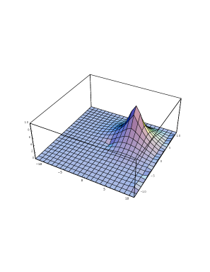
$(a)$       $(b)$

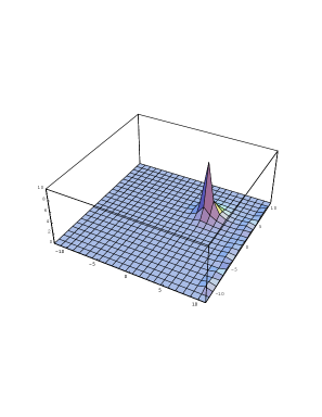
Figure 1: Numerical solutions of eq. (21) for $(a)$ small and $(b)$ large $g$, respectively. For the Bullough-Dodd case, eq. (29), the solutions are almost identical.

We can easily extend the previous analysis to the case in which $a$ contains several distinct zeroes. Simply find suitable approximate expressions for $\zeta$ near the zeroes of $a$ and apply the previous approximate analysis. The conclusion will be that the solution shrinks very quickly around the branch points as $g\to\infty$.

Let us briefly consider the case $N=3$. We have two fields $u_{1},u_{2}$ obeying the equations

$$\partial_{\zeta}\partial_{\bar{\zeta}}u_{1}+g^{2}\left(e^{-u_{1}-u_{2}}-e^{2u_{1}-u_{2}}\right)=-\frac{\pi}{3}\delta(a)~{}\partial_{\bar{\zeta}}a~{}\partial_{\zeta}\bar{a}$$

$$\partial_{\zeta}\partial_{\bar{\zeta}}u_{2}+g^{2}\left(e^{-u_{1}-u_{2}}-e^{2u_{2}-u_{1}}\right)=-\frac{\pi}{3}\delta(a)~{}\partial_{\bar{\zeta}}a~{}\partial_{\zeta}\bar{a}\,.$$

Subtracting one from the other we get an equation which is identically satisfied with $u_{1}=u_{2}$. The remaining equation for $u=u_{1}=u_{2}$ is

$$\partial_{\zeta}\partial_{\bar{\zeta}}u+g^{2}\left(e^{-2u}-e^{u}\right)=-\frac{\pi}{3}\delta(a)~{}\partial_{\bar{\zeta}}a~{}\partial_{\zeta}\bar{a}\,.$$ (29)

This is known as the Bullough–Dodd equation. The features of the solutions, with the present boundary conditions, are essentially the same as for the sinh–Gordon equation: for $g\to\infty$ they shrink around the zeroes of $a$. The numerical solutions do not differ significantly from the sinh–Gordon case.

We will not discuss the $N>3$ case here.

Appendix B Non–Cartan fluctuations

In this Appendix we briefly discuss the $Q_{\mathfrak{n}}$ term of the strong coupling action, i.e. the quadratic terms in the non–Cartan modes. $Q_{\mathfrak{n}}$ has the form

$$Q_{\mathfrak{n}}=\frac{1}{\pi}\int d^{2}w{\rm Tr}\left[\bar{x}^{\mathfrak{n}}{\cal Q}x^{\mathfrak{n}}+x^{I{\mathfrak{n}}}{\cal Q}x^{I{\mathfrak{n}}}+a_{\bar{w}}^{\mathfrak{n}}{\cal Q}a_{w}^{\mathfrak{n}}+\bar{c}^{\mathfrak{n}}{\cal Q}c^{\mathfrak{n}}+i(\theta_{s}^{\mathfrak{n}},\theta_{c}^{\mathfrak{n}}){\cal A}\left(\matrix{\theta_{s}^{\mathfrak{n}}\cr\theta_{c}^{\mathfrak{n}}\cr}\right)\right]\,,$$ (30)

where

$${\cal Q}={\rm ad}_{{\bar{X}}^{\circ}}\cdot{\rm ad}_{X^{\circ}}+{\rm ad}_{a_{\bar{w}}^{t}}\cdot{\rm ad}_{a_{w}^{t}}+{\rm ad}_{x^{It}}\cdot{\rm ad}_{x^{It}}$$

and

$${\cal A}=\left(\matrix{i{\rm ad}_{a_{\bar{w}}^{t}}&\gamma_{i}{\rm ad}_{X^{\circ i}}\cr\tilde{\gamma}_{i}{\rm ad}_{{\bar{X}}^{\circ i}}&i{\rm ad}_{a_{w}^{t}}\cr}\right)\,.$$

In the path integral we can now integrate over the non–Cartan modes and obtain a ratio of determinants of ${\cal A}$ and ${\cal Q}$. Since these operators do not have zero modes the calculation is elementary. The integration over $a^{\mathfrak{n}}$ and the conjugates exactly cancels the integration over $c^{\mathfrak{n}}$ and the conjugates. What remains is a ratio $\left(({\rm Det}{\cal A})^{16}/({\rm Det}{\cal Q})^{8}\right)^{N^{2}-N}$. The expression of the numerator is formal: one should understand ${{\rm Det}{\cal A}}$ as $\sqrt{{\rm Det}(-{\cal A}{\cal A}^{\dagger})}$. But ${\cal A}{\cal A}^{\dagger}={\cal A}^{\dagger}{\cal A}=-{\cal Q}$. Therefore the net result of integrating over the non–Cartan modes is 1. This is the result expected from supersymmetry in the absence of zero modes.

- [1] L. Motl, Proposals on Nonperturbative Superstring Interactions, hep-th/9701025.
- [2] T. Banks and N. Seiberg, Strings from Matrices, Nucl. Phys. B 497 (1997) 41 [hep-th/9702187].
- [3] W. Taylor, D-brane Field Theory on Compact Spaces, Phys. Lett. B 394 (1997) 283 [hep-th/9611042].
- [4] R. Dijkgraaf, E. Verlinde, H. Verlinde, Matrix String Theory, Nucl. Phys. B 500 (1997) 43 [hep-th/9703030].
- [5] R. Dijkgraaf, G. Moore, E. Verlinde, H. Verlinde, Elliptic Genera of Symmetric Products and Second Quantized Strings, Commun. Math. Phys. 185 (1997) 197 [hep-th/9608096].
- [6] H. Verlinde, A Matrix String Interpretation of the Large N Loop Equation, hep-th/9705029.
- [7] L. Bonora, C.S. Chu, On the String Interpretation of M(atrix) Theory, Phys. Lett. B 410 (1997) 142 [hep-th/9705137].
- [8] R. Dijkgraaf, E. Verlinde, H. Verlinde, Notes on Matrix and Microstrings, Nucl. Phys. 62 (Proc. Suppl.) (1998) 348 [hep-th/9709107].
- [9] S.B. Giddings, F. Hacquebord, H. Verlinde, High Energy Scattering of D–pair Creation in Matrix String Theory hep-th/9804121.
- [10] N.J. Hitchin, The self–duality equations on a Riemann surface, Proc. London Math. Soc. 55 (1987) 59; Lie groups and Teichmller space, Topology 31 (1992) 449.
- [11] N. Hitchin, Stable bundles and integrable systems, Duke Math. Jour. 54 (1987) 91.
- [12] T. Wynter, Gauge fields and interactions in matrix string theory Phys. Lett. B 415 (1997) 349 [hep-th/9709029].
- [13] G. Bonelli, L. Bonora and F. Nesti, Matrix string theory, instantons and affine Toda field theory [hep-th/9805071], to app. in Phys. Lett. B.
- [14] E. Gava, J.F. Morales, K.S. Narain, G. Thompson, Bound States of Type I D-Strings [hep-th/9801128]
- [15] M.B. Green, J.H. Schwarz, E. Witten, Superstring Theory, Cambridge Univ. Press, Cambridge 1987, vol. I.
- [16] E. Markman, Spectral curves and integrable systems, Comp. Math. 94 (1994) 255.
- [17] R. Donagi and E. Witten, Supersymmetric Yang–Mills theory and integrable systems, Nucl. Phys. B 460 (1996) 299 [hep-th/9510101].
- [18] S.B. Giddings and S.A. Wolpert, A triangulation of moduli space from light cone string theory Commun. Math. Phys. 109 (1987) 177.
- [19] E. Witten, On S–duality in abelian gauge theory hep-th/9505186.
- [20] L.L. Ahlfors, Open Riemann surfaces and extremal problems on compact subregions, Comm. Math. Helv. 24 (1950) 100. J.D. Fay, Theta functions on Riemann surfaces, Lect.Not.Math. Vol.352, Springer–Verlag, Berlin 1973.
- [21] S. Mandelstam, Dual resonance models, Phys. Rept. 13 (1974) 259.
- [22] J.-L. Gervais and B. Sakita, Extended particles in quantum field theories, Phys. Rev. D 11 (1975) 2943.
- [23] E. D’Hoker and D.H. Phong, The geometry of string perturbation theory, Rev. Mod. Phys. 60 (1988) 917.
- [24] T. Banks, W. Fischler, S.H. Shenker and L. Susskind, M Theory As A Matrix Model: A Conjecture, Phys. Rev. D 55 (1997) 5112 [hep-th/9610043].
- [25] L. Susskind, Another Conjecture about M(atrix) Theory, hep-th/9704080.
- [26] O.J. Ganor, S. Rangoolam and W. Taylor, Branes, fluxes and duality in M(atrix)–theory, Nucl. Phys. B 492 (1997) 191 [hep-th/9611202].
- [27] T. Banks, N. Seiberg and S. Shenker, Branes from matrices, Nucl. Phys. B 490 (1997) 91 [hep-th/9612157].
- [28] A.R. Its and V.Yu. Novokshenov, The isomonodromic deformation method in the theory of Painlevé equations, Lect. Notes Math. 1191, Springer–Verlag 1986.
- [29] B.Ye. Rusakov, Loop averages and partition functions in U(N) gauge theory on two-dimensional manifolds, Mod. Phys. Lett. A 5 (1990) 693.