NBI-HE-98-18

July 1998

Abstract

The meander problem is a combinatorial problem which provides a toy model of the compact folding of polymer chains. In this paper we study various questions relating to the enumeration of meander diagrams, using diagrammatical methods. By studying the problem of folding tree graphs, we derive a lower bound on the exponential behaviour of the number of connected meander diagrams. A different diagrammatical method, based on a non-commutative algebra, provides an approximate calculation of the behaviour of the generating functions for both meander and semi-meander diagrams.

Keywords: meander, folding, combinatorial

1 Introduction

The problem of enumerating meander and semi-meander diagrams has appeared in many diverse areas of mathematics [1, 2] and computer science [3, 4]. In the case of semi-meanders it can be reformulated as an enumeration of the foldings of a strip of postage stamps [5, 6], which is equivalent to a model of compact foldings of a polymer. Thus the semi-meanders serve as a toy model of the statistical mechanics of such polymer chains.

The generating function for meanders can be written as an Hermitian matrix model or as a supersymmetric matrix model [7, 8]. Alternatively combinatorial methods can be used [5, 6], one can represent the problem in terms of non-commuting variables [8] or using a Temperley-Lieb algebra [9, 10, 11]. Despite all of these different approaches and the initial apparent simplicity of the problem, the task of counting the meander and semi-meander diagrams has remained largely unsolved.

In this paper we apply diagrammatical methods to the study of meanders. In section 2 the problem is defined and some tables of meander numbers are given. Then in section 3 we calculate bounds on the number of connected meanders, in particular the lower bound is improved by mapping the meanders to folded tree graphs. Section 4 uses a diagrammatic representation of a non-commutative algebra to calculate approximate generating functions for meanders and semi-meanders. The nature of the phase transition for semi-meanders is also considered in this section. Finally we give our conclusions in section 5 of the paper.

2 Definition of the meander numbers

2.1 Meanders

Suppose that we have an infinite line (or “river”) on a planar surface. Then a connected meander of order $n$ is defined to be a non-self-intersecting connected loop (or “road”) which crosses the river $2n$ times (the crossing points are referred to as “bridges”). Two meanders are considered to be equivalent if it is possible to smoothly deform one meander into the other without changing the number of bridges during the process. The total number of inequivalent connected meanders of order $n$ is denoted $M^{(1)}_{n}$, and we can define a generating function, $M(x)$ for connected meanders,

$$M(x)=\sum_{n=1}^{\infty}M^{(1)}_{n}\ x^{n}.$$ (1)

The first few meander numbers are $M^{(1)}_{1}=1$, $M^{(1)}_{2}=2$ and $M^{(1)}_{3}=8$. Figure 1 shows some simple meander diagrams.

Figure 1: Some simple meander diagrams.

The definition can be extended to include cases in which the road consists of $k$ disconnected parts, giving a number of meanders of order $n$ denoted by $M^{(k)}_{n}$. This leads us to define a more general generating function,

$$M(x,m)=\sum_{n=1}^{\infty}\sum_{k=1}^{n}M^{(k)}_{n}\ x^{n}m^{k}.$$ (2)

Table 1 gives $M^{(k)}_{n}$ for small values of $k$ and $n$ (these numbers are taken from [6]). Some examples of disconnected meanders are shown in figure 2.

Figure 2: Some simple disconnected meander diagrams.

$k$	$n=$ 1	2	3	4	5	6	7
1	1	2	8	42	262	1828	13820
2		2	12	84	640	5236	45164
3			5	56	580	5894	60312
4				14	240	3344	42840
5					42	990	17472
6						132	4004
7							429

Table 1: Meander numbers, $M^{(k)}_{n}$ (from ref. [6]).

2.2 Semi-meanders

Suppose that instead of having an infinite river we have only a semi-infinite river. The end of the river is often referred to as the “source”. In this case the road can wrap around the source of the river and the corresponding diagrams are called “semi-meanders”. As before two semi-meanders are equivalent if one can be smoothly deformed into the other, without changing the number of bridges. Figure 3 shows some examples of semi-meanders.

Figure 3: Some semi-meander diagrams. The source is marked with a dot.

Let us denote the number of inequivalent semi-meanders with $n$ bridges and a road consisting of $k$ connected parts, as $\overline{M}^{(k)}_{n}$. Then the corresponding generating function is

$$S(c,m)=\sum_{n=1}^{\infty}\sum_{k=1}^{n}\overline{M}^{(k)}_{n}c^{n}m^{k}.$$ (3)

Note that the meanders can only have an even number of bridges, whereas semi-meanders can have both even and odd numbers of bridges. This is the reason for the slightly different definitions of the generating functions and one should define $x\equiv c^{2}$. Table 2 gives the numbers for the simplest semi-meanders.

$k$	$n=$ 1	2	3	4	5	6	7
1	1	1	2	4	10	24	66
2		1	2	6	16	48	140
3			1	3	11	37	126
4				1	4	17	66
5					1	5	24
6						1	6
7							1

Table 2: Semi-meander numbers, $\overline{M}^{(k)}_{n}$ (from ref. [6]).

3 Connected meanders

3.1 Bounds on the number of meanders

In this section we will derive some bounds on the number of inequivalent connected meanders (from now on it should be understood that we are referring always to inequivalent meanders). The standard way of doing this is to consider a meander as being formed from two arch diagrams (see figure 4 for some examples of arch diagrams). That is, if we take a meander diagram and cut it in two along the river, then this gives one arch diagram above the river and one below it (see figure 5).

Figure 4: Two example arch diagrams.

Figure 5: A meander cut into two sets of arches.

An arch diagram of order $n$ consists of $2n$ points arranged in a line, which are connected up in pairs by drawing $n$ arches above the points. The arches are not allowed to intersect each other and each point has exactly one arch joined to it. The number of inequivalent order $n$ arch configurations is denoted $A_{n}$, and the generating function for arches is defined as

$$A(c)=\sum_{n=0}^{\infty}A_{n}c^{n},\qquad\qquad A_{0}\equiv 1.$$ (4)

The empty arch diagram $A_{0}$ has the value $1$. A non-empty arch diagram can be decomposed into two arch diagrams separated by the arch connected to the rightmost point. This is illustrated diagrammatically as . That is, $A(c)$ satisfies the equation

$$A=1+cA^{2}.$$ (5)

Hence

$$A(c)=\frac{1}{2c}\left(1-\sqrt{1-4c}\right)$$ (6)

and

$$A_{n}=\frac{(2n)!}{n!(n+1)!}\quad{\mathop{\sim}\limits_{\scriptscriptstyle n\to\infty}}\quad\frac{4^{n}}{n^{3/2}}.$$ (7)

In fact $A_{n}$ is equal to $c_{n}$, the Catalan number of order $n$.

Since gluing together two arch configurations of order $n$ gives a (possibly disconnected) meander of order $n$ we have

$$M^{(1)}_{n}\leq\sum_{k=1}^{n}M^{(k)}_{n}={A_{n}}^{2}.$$ (8)

In fact, given an arch diagram on top, we can always find an arch configuration on the bottom that creates a connected meander (using the algorithm given in fig. 21 of ref. [6]), which means that $A_{n}\leq M^{(1)}_{n}$.

Consider the asymptotics of $M^{(1)}_{n}$ for a large number of bridges,

$$M^{(1)}_{n}\quad{\mathop{\sim}\limits_{\scriptscriptstyle n\to\infty}}\quad{\it const.}\ \frac{R^{2n}}{n^{\alpha}},$$ (9)

where $R$ gives the exponential behaviour and $\alpha$ is a configuration exponent. Then

$$A_{n}\leq M^{(1)}_{n}\leq{A_{n}}^{2}$$ (10)

implies that

$$2\leq R\leq 4.$$ (11)

3.2 Improved lower bound

The contents of the previous section are all well-known. In this section we would like to improve the lower bound on $R$. Instead of considering arch diagrams we will rewrite the connected meanders as tree diagrams.

The road of a connected meander divides the plane into two parts: an inside and an outside. Smoothly deforming the road in such a way as to reduce the inside area towards zero yields, in the limit, a connected tree graph (see fig. 6). Given such a folded tree graph we can easily reconstruct the corresponding meander.

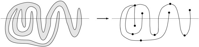
Figure 6: Converting a connected meander, with the inside shaded, to a (folded) tree diagram.

Note that applying this procedure to a disconnected meander would yield a graph that is disconnected and/or contains loops. The tree graphs corresponding to connected meanders can have vertices of arbitrary coordination number, and the mapping procedure is defined such that adjacent vertices on the tree occur above and below the river in an alternating fashion. There is a one-to-one correspondence between such tree graphs and the set of connected meanders. By putting bounds on the number of such trees we will improve the lower bound on $R$ discussed in the previous section.

It is convenient to label the vertices of each tree with either an ’A’ or ’B’, signifying that they are above or below the river respectively. The left-most link in the tree will be marked by drawing it thicker. Each tree can then be unfolded as shown in figure 7.

Figure 7: An unfolded tree diagram corresponding to the folded tree in fig. 6.

In general an unfolded tree has many different ways of folding it, subject to the constraints that when folded the ’A’ vertices are above the line and the ’B’ vertices are below it, and that the marked link is leftmost. For example, figure 7 can be refolded as in figure 8. Each unfolded tree has at least one possible folding and usually has many more. Thus each unfolded tree represents a whole class of connected meander diagrams.

Figure 8: Another more regular folding of the tree diagram.

By counting the number of unfolded trees we will generate a lower bound on the number of connected meanders.

A rooted tree with arbitrary coordination numbers can be generated using the relation illustrated in fig. 9. That is, if each link in the tree is weighted with $x$, then the generating function for trees, $T(x)$, satisfies

$$T(x)=x(1+T+T^{2}+T^{3}+\cdots)=x/(1-T)$$ (12)

and hence

$$T(x)=\frac{1}{2}\left(1-\sqrt{1-4x}\right).$$ (13)

Figure 9: Relation which determines $T(x)$, the generating function for rooted trees with arbitrary coordination numbers.

Unfolded trees have a generating function $U(x)$, which from fig. 10 is given by

$$U(x)=\frac{x}{(1-T)^{2}}.$$ (14)

Hence

$$U(x)=\frac{T^{2}}{x}=\frac{1}{2x}\left(1-\sqrt{1-4x}\right)-1=A(x)-1,$$ (15)

with $A(x)$ defined through equation (6). So we have

$$U(x)=\sum_{n=1}^{\infty}A_{n}x^{n}.$$ (16)

Figure 10: Relation which determines $U(x)$, the generating function for unfolded trees.

However, as mentioned earlier, the number of unfolded trees (with $n$ links) gives a lower bound on the number of connected meanders (with $2n$ bridges), that is, $A_{n}\leq M^{(1)}_{n}$ and $R\geq 2$. This reproduces the result in section 3.1. Note that since each link of the tree graph is equivalent to two bridges in the corresponding connected meander (fig. 6), the factor for links in the tree had to be $x$ for consistency with the definitions in section 2.

The representation in terms of trees allows us to improve on the bound by counting more of the possible foldings for each unfolded tree. Suppose that the generating function for partially folded trees is denoted by $\Theta(x)$,

$$\Theta(x)\equiv\sum_{n=1}^{\infty}\Theta_{n}x^{n},$$ (17)

where by partially folded trees, it is meant that only some of the possible foldings are included for each unfolded tree. That is, we are summing over all the trees in $U(x)$, but only some of the foldings. Thus we will have $A_{n}\leq\Theta_{n}\leq M^{(1)}_{n}$. Let us now define $\Theta(x)$ and hence the subset of the possible foldings that are included in the partial folding. First, the relation in fig. 10 is rewritten to include more foldings

Figure 11: Relation which determines $\Theta(x)$, the generating function for partially folded trees.

(see fig. 11). The rooted trees $T(x)$ have been replaced by $V(x)$, which is more folded that $T$ and is defined below. The sum is over all possible ways of interleaving the arbitrary number of $V$-trees. This relation gives

$$\Theta(x)=\frac{x}{1-2V},$$ (18)

where the $x$ comes from the marked link. The $(1-2V)^{-1}$ factor is due to the sum over all possible numbers of $V$-trees, with each tree being connected to one of 2 vertices (’A’ or ’B’).

Now consider redrawing the relation in fig. 9 as shown in fig. 12.

Figure 12: The relation determining $T(x)$, which has been rewritten.

Then we see that the generating function for $T$ only folds in one direction, but that more foldings can be included if we fold to both left and right. Thus for $V(x)$ the relation in fig. 13 will be used instead. Figure 14 shows a typical $V$-tree.

Figure 13: Relation which determines $V(x)$.

Figure 14: A typical $V$-tree contained in $V(x)$.

Thus we have

$$V(x)=x\left(1+2V+3V^{2}+4V^{3}+\cdots\right)=\frac{x}{(1-V)^{2}}.$$ (19)

Diagrams such as that in fig. 15 are generated when this generating function for $V(x)$ is inserted in to (18).

Figure 15: Example of a diagram included in $\Theta(x)$.

Thus $\Theta(x)$ will contain a large number, but my no means all, of the possible folded tree diagrams. As $x$ is increased from zero it reaches some critical value $x_{c}$ at which $\Theta(x)$ is non-analytic. This is caused by the critical behaviour of $V(x)$ due to $\frac{dV}{dx}$ diverging as $x\to x_{c}$. Now,

$$\frac{dV}{dx}=\frac{1}{(1-4V+3V^{2})},$$ (20)

so that $V(x_{c})=\frac{1}{3}$ and $x_{c}=\frac{4}{27}$. Thus

$$\Theta_{n}\sim\left(\frac{27}{4}\right)^{n}$$ (21)

and hence $R\geq\frac{3\sqrt{3}}{2}\approx 2.598$. This improves the bound given previously.

3.3 Further improvement to lower bound

The lower bound can be improved further by including more foldings than exist in the generating function for $V(x)$. If $V(x)$ is replaced by $W(x)$, whose generating function is given by the relation in fig. 16, then an improved generating function is

$$\Theta_{imp.}(x)=\frac{x}{1-2W},$$ (22)

where

$$W(x)=\frac{x}{(1-\frac{W}{1-W})^{2}}=x\frac{(1-W)^{2}}{(1-2W)^{2}}.$$ (23)

The generating function for $W(x)$ includes all the trees contained in $V(x)$, but also trees in which there are arbitrary numbers of $W$-trees (emerging from the root) interleaved with the branches connected to the vertex. Replacing $V$ by $W$ in (19) and then changing $W$ to $W/(1-W)$ on the right hand side gives (23). This last replacement takes into account the fact that each branch in fig. 13 now has an arbitrary number of trees inserted between it and the previous branch or trunk. Figure 17 shows a typical diagram included in $W(x)$.

Figure 16: Relation which determines $W(x)$, where we are summing over arbitrary numbers of $W$-trees inserted below each branch.

Figure 17: Typical diagram contained in $W(x)$. The root link of the tree is drawn thicker. The links which occur in a $W$-tree, but not a $V$-tree are drawn dotted.

Equation (23) gives

$$\frac{dW}{dx}=\frac{(1-W)^{2}}{(1-8W+12W^{2}-2x(W-1))}.$$ (24)

It is the divergence of this derivative which defines the critical value of $x$,

$$x_{c}=\frac{1}{8}\left(71-17\sqrt{17}\right)$$ (25)

and hence the lower bound on $R$ is

$$R\geq{x_{c}}^{-\frac{1}{2}}\approx 2.970.$$ (26)

This is a significant improvement over the lower bound $R\geq 2$ that we had initially. It is worth noting that computer enumerations of the number of semi-meanders yield an estimated value of $R\approx 3.50$ (see reference [12]). A power series expansion of $\Theta_{imp.}(x)$ gives

$$\Theta_{imp.}(x)=x+2x^{2}+8x^{3}+42x^{4}+\underline{252}x^{5}+\underline{1636}x^{6}+\cdots,$$ (27)

which should be compared with the correct series for meander diagrams

$$M(x)=x+2x^{2}+8x^{3}+42x^{4}+262x^{5}+1828x^{6}+\cdots.$$ (28)

The two series agree up to and including terms of order $x^{4}$, after which we see that $\Theta_{imp.}(x)$ is, as expected, undercounting the number of meander graphs (the relevant terms in $\Theta_{imp.}$ are underlined). In principle one could improve the generating functions $\Theta_{imp.}(x)$ and $W(x)$ in order to raise the lower bound further, however it appears to require increasing amounts of effort for diminishing returns.

4 Diagrammatic method

In this section, we will develop a diagrammatic method for generating meander and semi-meander diagrams. By truncating some of the equations, we will derive approximate solutions for the critical behaviour of $M(x,m)$ and $S(c,m)$, which can be compared with results from computer enumerations carried out by other authors.

4.1 $u$-diagrams

Following reference [8], let us introduce a set of non-commuting variables $\{u_{a},u_{a}^{\dagger}\}$ with $a=1,\cdots,m$, which obey the relation

$$u_{a}u_{b}^{\dagger}=\delta_{ab}.$$ (29)

We will consider $u_{a}$, $u_{a}^{\dagger}$ as annihilation and creation operators in some Hilbert space, with a vacuum $|\Omega\rangle$, such that

$$u_{a}|\Omega\rangle=0,\qquad\qquad\langle\Omega|u_{b}^{\dagger}=0,\qquad\qquad\langle\Omega|\Omega\rangle=1.$$ (30)

Now define $G$ and $G^{\dagger}$ by

$$G = 1+c\ Gu_{a}Gu_{a}$$ (31)

$$G^{\dagger} = 1+c\ u_{a}^{\dagger}G^{\dagger}u_{a}^{\dagger}G^{\dagger},$$

where we are summing over the repeated index $a$ ($a=1,\cdots,m$). Diagrammatically we can write the first equation as , where a line emerging from an ’$a$’, that is written below the equation, represents $u_{a}$. The fact that the two lines are joined into an arch indicates that we are summing over the repeated index ’$a$’. Since ’$a$’ is just a dummy index it can be omitted. It is to be understood that each arch has a factor of $c$ associated with it. Expanding this equation gives

$$G^{\phantom{\dagger}}=1+\begin{picture}(40.0,30.0)\put(20.0,0.0){\oval(30.0,60.0)[t]} \end{picture}+\begin{picture}(40.0,30.0)\put(20.0,0.0){\oval(30.0,60.0)[t]} \end{picture}\begin{picture}(40.0,30.0)\put(20.0,0.0){\oval(30.0,60.0)[t]} \end{picture}+\begin{picture}(56.0,50.0)\put(28.0,0.0){\oval(46.0,90.0)[t]} \put(28.0,0.0){\oval(24.0,55.0)[t]} \end{picture}+\begin{picture}(40.0,30.0)\put(20.0,0.0){\oval(30.0,60.0)[t]} \end{picture}\begin{picture}(40.0,30.0)\put(20.0,0.0){\oval(30.0,60.0)[t]} \end{picture}\begin{picture}(40.0,30.0)\put(20.0,0.0){\oval(30.0,60.0)[t]} \end{picture}+\begin{picture}(40.0,30.0)\put(20.0,0.0){\oval(30.0,60.0)[t]} \end{picture}\begin{picture}(56.0,50.0)\put(28.0,0.0){\oval(46.0,90.0)[t]} \put(28.0,0.0){\oval(24.0,55.0)[t]} \end{picture}+\begin{picture}(56.0,50.0)\put(28.0,0.0){\oval(46.0,90.0)[t]} \put(28.0,0.0){\oval(24.0,55.0)[t]} \end{picture}\begin{picture}(40.0,30.0)\put(20.0,0.0){\oval(30.0,60.0)[t]} \end{picture}+\begin{picture}(70.0,50.0)\put(35.0,0.0){\oval(60.0,90.0)[t]} \put(22.0,0.0){\oval(20.0,45.0)[t]} \put(48.0,0.0){\oval(20.0,45.0)[t]} \end{picture}+\begin{picture}(70.0,50.0)\put(35.0,0.0){\oval(60.0,90.0)[t]} \put(35.0,0.0){\oval(40.0,60.0)[t]} \put(35.0,0.0){\oval(20.0,40.0)[t]} \end{picture}+\cdots,$$ (32)

that is, $G=1+u_{a}u_{a}+u_{a}u_{a}u_{b}u_{b}+u_{a}u_{b}u_{b}u_{a}+\cdots$. Thus $G$ generates arch configurations, however unlike $A$ in equation (5) $G$ keeps track of where the ends of the arches are positioned. The generating function $G^{\dagger}$ generates arch configurations in terms of $u_{a}^{\dagger}$, diagrammatically one can consider these as inverted arch diagrams. So

$$G^{\dagger}=1+\begin{picture}(40.0,30.0)(0.0,-30.0)\put(20.0,0.0){\oval(30.0,60.0)[b]} \end{picture}+\begin{picture}(40.0,30.0)(0.0,-30.0)\put(20.0,0.0){\oval(30.0,60.0)[b]} \end{picture}\begin{picture}(40.0,30.0)(0.0,-30.0)\put(20.0,0.0){\oval(30.0,60.0)[b]} \end{picture}+\begin{picture}(56.0,50.0)(0.0,-30.0)\put(28.0,0.0){\oval(46.0,90.0)[b]} \put(28.0,0.0){\oval(24.0,55.0)[b]} \end{picture}+\begin{picture}(40.0,30.0)(0.0,-30.0)\put(20.0,0.0){\oval(30.0,60.0)[b]} \end{picture}\begin{picture}(40.0,30.0)(0.0,-30.0)\put(20.0,0.0){\oval(30.0,60.0)[b]} \end{picture}\begin{picture}(40.0,30.0)(0.0,-30.0)\put(20.0,0.0){\oval(30.0,60.0)[b]} \end{picture}+\begin{picture}(40.0,30.0)(0.0,-30.0)\put(20.0,0.0){\oval(30.0,60.0)[b]} \end{picture}\begin{picture}(56.0,50.0)(0.0,-30.0)\put(28.0,0.0){\oval(46.0,90.0)[b]} \put(28.0,0.0){\oval(24.0,55.0)[b]} \end{picture}+\begin{picture}(56.0,50.0)(0.0,-30.0)\put(28.0,0.0){\oval(46.0,90.0)[b]} \put(28.0,0.0){\oval(24.0,55.0)[b]} \end{picture}\begin{picture}(40.0,30.0)(0.0,-30.0)\put(20.0,0.0){\oval(30.0,60.0)[b]} \end{picture}+\begin{picture}(70.0,50.0)(0.0,-30.0)\put(35.0,0.0){\oval(60.0,90.0)[b]} \put(22.0,0.0){\oval(20.0,45.0)[b]} \put(48.0,0.0){\oval(20.0,45.0)[b]} \end{picture}+\begin{picture}(70.0,50.0)(0.0,-30.0)\put(35.0,0.0){\oval(60.0,90.0)[b]} \put(35.0,0.0){\oval(40.0,60.0)[b]} \put(35.0,0.0){\oval(20.0,40.0)[b]} \end{picture}+\cdots.$$ (33)

The dagger operator acting on a diagram can be thought of as reflecting the diagram, for example,

$$\left[\begin{picture}(40.0,30.0)\put(20.0,0.0){\oval(30.0,60.0)[t]} \end{picture}\begin{picture}(56.0,50.0)\put(28.0,0.0){\oval(46.0,90.0)[t]} \put(28.0,0.0){\oval(24.0,55.0)[t]} \end{picture}\right]^{\dagger}=\begin{picture}(40.0,30.0)(0.0,-30.0)\put(20.0,0.0){\oval(30.0,60.0)[b]} \end{picture}\begin{picture}(56.0,50.0)(0.0,-30.0)\put(28.0,0.0){\oval(46.0,90.0)[b]} \put(28.0,0.0){\oval(24.0,55.0)[b]} \end{picture}.$$ (34)

Now consider the expression $GG^{\dagger}$, this contains terms of the form $u_{a_{1}}u_{a_{2}}\!\!\cdots u_{a_{n}}u_{b_{n}}^{\dagger}u_{b_{n-1}}^{\dagger}\!\!\!\!\!\!\cdots u_{b_{1}}^{\dagger}$. When this term is drawn as a diagram the inverted arches can be drawn under the upright arches to make the connection with meander diagrams clear. One can apply equation (29) repeatedly to eliminate $u$ and $u^{\dagger}$ variables. In terms of diagrams this corresponds to gluing together a leg on the upright arch diagram to one on the inverted diagram (see fig. 18). If the number of $u$ variables is equal to the number of $u^{\dagger}$ variables then we will end up with a (possibly disconnected) meander diagram. However, if the numbers are not equal then there will be spare $u$ or $u^{\dagger}$ left over. Taking the vacuum expectation value will kill these extra terms and hence $\langle GG^{\dagger}\rangle$ generates all the meander diagrams, since any meander can be made by gluing together two arch diagrams. Each closed loop in the meander diagram will give a factor of $\delta_{aa}=m$. Thus the correct weightings are generated and hence

$$\langle GG^{\dagger}\rangle=1+M(x,m).$$ (35)

Figure 18: (a) Applying equation (29) to $u_{a_{1}}\cdots u_{a_{n}}u_{b_{n}}^{\dagger}\!\!\!\cdots u_{b_{1}}^{\dagger}$.   (b) Applying equation (29) twice to a term in $GG^{\dagger}$.

4.2 $X$-diagrams

It is convenient now to introduce a new set of variables, $\{X_{a},X_{a}^{\dagger}\}$, defined by

$$X_{a}=\frac{Gu_{a}}{\sqrt{m}},\qquad\qquad X_{a}^{\dagger}=\frac{u_{a}^{\dagger}G^{\dagger}}{\sqrt{m}}.$$ (36)

So that

$$|{\bf X}|^{2}\equiv\sum_{a=1}^{m}X_{a}X_{a}^{\dagger}=GG^{\dagger},$$ (37)

$$\left\langle|{\bf X}|^{2}\right\rangle=1+M(x,m).$$ (38)

The equations for $X_{a}$ equivalent to (29) and (30) are

$$X_{a}X_{b}^{\dagger}=\frac{1}{m}\delta_{ab}|{\bf X}|^{2},$$ (39)

$$X_{a}|\Omega\rangle=0,\qquad\qquad\langle\Omega|X_{b}^{\dagger}=0,\qquad\qquad\langle\Omega|\Omega\rangle=1.$$ (40)

From (31) we have

$$|{\bf X}|^{2} = \left(1+cmX_{a}X_{a}\right)\left(1+cmX_{b}^{\dagger}X_{b}^{\dagger}\right)$$ (41)

$$= 1+cm\left(X_{a}X_{a}+X_{a}^{\dagger}X_{a}^{\dagger}\right)+c^{2}mX_{a}|{\bf X}|^{2}X_{a}^{\dagger},$$ (42)

where repeated indices are summed over. In a similar fashion to the $u,u^{\dagger}$ diagrams, this can be written diagrammatically, in this case as

$$\begin{picture}(40.0,40.0)\put(20.0,0.0){\oval(30.0,60.0)[t]} \put(20.0,0.0){\line(0,1){40.0} } \end{picture}=1+cm\left(\begin{picture}(40.0,30.0)\put(20.0,0.0){\oval(30.0,60.0)[t]} \end{picture}\ \line(0,1){40.0}+\line(0,1){40.0}\ \begin{picture}(40.0,30.0)\put(20.0,0.0){\oval(30.0,60.0)[t]} \end{picture}\right)+c^{2}m\ \begin{picture}(56.0,50.0)\put(28.0,0.0){\oval(46.0,90.0)[t]} \put(28.0,0.0){\oval(24.0,55.0)[t]} \put(28.0,0.0){\line(0,1){60.0} } \end{picture},$$ (43)

where the ends corresponding to non-daggered operators are on the left of the vertical line and those for the daggered operators are on the right. Two ends are joined into an arch whenever the corresponding operators share a summed over index. The vertical line is only present in order to indicate the boundary between non-daggered and daggered operators. Equation (39) implies that

$$X_{a}X_{a}X_{b}^{\dagger}X_{b}^{\dagger}=\frac{1}{m}\left(X_{a}X_{c}X_{c}^{\dagger}X_{a}^{\dagger}\right),$$ (44)

which was used above, and

$$X_{b}X_{a}X_{a}X_{b}^{\dagger}=\frac{1}{m}\left(X_{a}X_{a}X_{c}X_{c}^{\dagger}\right),$$ (45)

which can be drawn respectively as

$$\begin{picture}(40.0,30.0)\put(20.0,0.0){\oval(30.0,60.0)[t]} \end{picture}\ \line(0,1){40.0}\ \begin{picture}(40.0,30.0)\put(20.0,0.0){\oval(30.0,60.0)[t]} \end{picture}=\frac{1}{m}\begin{picture}(56.0,50.0)\put(28.0,0.0){\oval(46.0,90.0)[t]} \put(28.0,0.0){\oval(24.0,55.0)[t]} \put(28.0,0.0){\line(0,1){60.0} } \end{picture}$$ (46)

and

$$\begin{picture}(90.0,50.0)\put(45.0,0.0){\oval(80.0,90.0)[t]} \put(35.0,0.0){\oval(24.0,55.0)[t]} \put(65.0,0.0){\line(0,1){60.0} } \end{picture}=\frac{1}{m}\begin{picture}(40.0,30.0)\put(20.0,0.0){\oval(30.0,60.0)[t]} \end{picture}\begin{picture}(40.0,40.0)\put(20.0,0.0){\oval(30.0,60.0)[t]} \put(20.0,0.0){\line(0,1){40.0} } \end{picture}\ .$$ (47)

In principle one could repeatedly substitute equation (42) into itself in order to expand $|{\bf X}|^{2}$ in terms of $X_{a}$ and $X_{a}^{\dagger}$. However this rapidly becomes tedious and it is necessary to find a simpler way of calculating $|{\bf X}|^{2}$. Let us define $\{A_{n}\}$ by

$$A_{0}=1,\qquad\qquad A_{1}=\begin{picture}(40.0,40.0)\put(20.0,0.0){\oval(30.0,60.0)[t]} \put(20.0,0.0){\line(0,1){40.0} } \end{picture},\qquad\qquad A_{2}=\begin{picture}(56.0,50.0)\put(28.0,0.0){\oval(46.0,90.0)[t]} \put(28.0,0.0){\oval(24.0,55.0)[t]} \put(28.0,0.0){\line(0,1){60.0} } \end{picture},\qquad\qquad A_{3}=\begin{picture}(70.0,55.0)\put(35.0,0.0){\oval(60.0,100.0)[t]} \put(35.0,0.0){\oval(40.0,70.0)[t]} \put(35.0,0.0){\oval(20.0,50.0)[t]} \put(35.0,0.0){\line(0,1){60.0} } \end{picture},\ \ \cdots\$$ (48)

and $\{Y_{n}\}$ by

$$Y_{1}=cm\left(\begin{picture}(40.0,30.0)\put(20.0,0.0){\oval(30.0,60.0)[t]} \end{picture}\ \line(0,1){40.0}+\line(0,1){40.0}\ \begin{picture}(40.0,30.0)\put(20.0,0.0){\oval(30.0,60.0)[t]} \end{picture}\right),\qquad\qquad\begin{picture}(220.0,60.0)\put(160.0,0.0){\oval(120.0,100.0)[t]} \put(0.0,0.0){$Y_{n}=\ \ Y_{n-1}\ \ $} \end{picture}\ .$$ (49)

For later use we will define the following notation, that  is an operator, which multiplies the expression following it by $X_{a}X_{a}$ (that is, ) on the left-hand side, whereas  multiplies the expressing following it by $X_{a}^{\dagger}X_{a}^{\dagger}$ on the right-hand side. Thus,

$$Y_{1}=cm\left(\begin{picture}(40.0,30.0)\put(20.0,0.0){\oval(30.0,60.0)[t]} \end{picture}\ \line(0,1){40.0}+\line(0,1){40.0}\ \begin{picture}(40.0,30.0)\put(20.0,0.0){\oval(30.0,60.0)[t]} \end{picture}\right)=cm\left(\begin{picture}(40.0,40.0)\put(20.0,0.0){\oval(30.0,50.0)[t]} \put(0.0,30.0){$\rightarrow$} \end{picture}\ +\begin{picture}(40.0,40.0)\put(20.0,0.0){\oval(30.0,50.0)[t]} \put(0.0,30.0){$\leftarrow$} \end{picture}\ \right)\line(0,1){40.0}\$$ (50)

and

$$Y_{2}=c\left(\begin{picture}(40.0,30.0)\put(20.0,0.0){\oval(30.0,60.0)[t]} \end{picture}\begin{picture}(40.0,40.0)\put(20.0,0.0){\oval(30.0,60.0)[t]} \put(20.0,0.0){\line(0,1){40.0} } \end{picture}+\begin{picture}(40.0,40.0)\put(20.0,0.0){\oval(30.0,60.0)[t]} \put(20.0,0.0){\line(0,1){40.0} } \end{picture}\begin{picture}(40.0,30.0)\put(20.0,0.0){\oval(30.0,60.0)[t]} \end{picture}\right)=c\left(\begin{picture}(40.0,40.0)\put(20.0,0.0){\oval(30.0,50.0)[t]} \put(0.0,30.0){$\rightarrow$} \end{picture}\ +\begin{picture}(40.0,40.0)\put(20.0,0.0){\oval(30.0,50.0)[t]} \put(0.0,30.0){$\leftarrow$} \end{picture}\ \right)\begin{picture}(40.0,40.0)\put(20.0,0.0){\oval(30.0,60.0)[t]} \put(20.0,0.0){\line(0,1){40.0} } \end{picture}\ .$$ (51)

Now equation (43) can also be written as

$$A_{1}=1+Y_{1}+\alpha A_{2},$$ (52)

where $\alpha\equiv c^{2}m=xm$. This equation generalizes to

$$A_{n}=A_{n-1}+Y_{n}+\alpha A_{n+1}.$$ (53)

Note that we wish to evaluate $\left\langle A_{1}\right\rangle$ since

$$\left\langle A_{1}\right\rangle=\left\langle\begin{picture}(40.0,40.0)\put(20.0,0.0){\oval(30.0,60.0)[t]} \put(20.0,0.0){\line(0,1){40.0} } \end{picture}\right\rangle=\left\langle|{\bf X}|^{2}\right\rangle=\left\langle GG^{\dagger}\right\rangle=1+M(x,m).$$ (54)

The next step is to rewrite $A_{1}$ in terms of $\{Y_{n}\}$ and $\alpha$. We rewrite (53) as

$$0=\alpha\left(A_{n+1}-fA_{n}\right)-\frac{1}{f}\left(A_{n}-fA_{n-1}\right)+Y_{n},$$ (55)

where $f(\alpha)$ is given by

$$\alpha f+\frac{1}{f}=1,\qquad\qquad f(\alpha)=\frac{1}{2\alpha}\left(1-\sqrt{1-4\alpha}\right)$$ (56)

and define $\overline{A}_{n}$ by

$$\overline{A}_{n}=A_{n}-fA_{n-1}.$$ (57)

Then from (55)

$$\overline{A}_{n}=fY_{n}+\alpha f\overline{A}_{n+1}.$$ (58)

This yields immediately

$$A_{1}=f+\overline{A}_{1}=f.\left(1+Y_{1}+(\alpha f)Y_{2}+(\alpha f)^{2}Y_{3}+\cdots\right).$$ (59)

The first term in $\left\langle A_{1}\right\rangle$ is $f(\alpha)$, which generates the Catalan numbers (see equation (6)). These correspond to the set of numbers $M_{n}^{(n)}$ in $M(x,m)$, that is, the leading diagonal of table 1.

4.3 Calculation of $\left\langle Y_{n}\right\rangle$

In order to calculate $\left\langle A_{1}\right\rangle$, or at least an approximation to it, we need to consider how to calculate $\left\langle Y_{n}\right\rangle$. It is worth noting that $\left\langle Y_{1}\right\rangle=0$ from (40).

Now consider $Y_{2}$,

$$Y_{2}=c\Bigl{(}\begin{picture}(40.0,40.0)\put(20.0,0.0){\oval(30.0,50.0)[t]} \put(0.0,30.0){$\rightarrow$} \end{picture}\ \!+\begin{picture}(40.0,40.0)\put(20.0,0.0){\oval(30.0,50.0)[t]} \put(0.0,30.0){$\leftarrow$} \end{picture}\ \!\Bigr{)}A_{1}=cf\Bigl{(}\begin{picture}(40.0,40.0)\put(20.0,0.0){\oval(30.0,50.0)[t]} \put(0.0,30.0){$\rightarrow$} \end{picture}\ \!+\begin{picture}(40.0,40.0)\put(20.0,0.0){\oval(30.0,50.0)[t]} \put(0.0,30.0){$\leftarrow$} \end{picture}\ \!\Bigr{)}\left(1+Y_{1}+(\alpha f)Y_{2}+(\alpha f)^{2}Y_{3}+\cdots\right),$$ (60)

so that

$$Y_{2}=\left(1-c\alpha f^{2}\Bigl{(}\begin{picture}(40.0,40.0)\put(20.0,0.0){\oval(30.0,50.0)[t]} \put(0.0,30.0){$\rightarrow$} \end{picture}\ \!+\begin{picture}(40.0,40.0)\put(20.0,0.0){\oval(30.0,50.0)[t]} \put(0.0,30.0){$\leftarrow$} \end{picture}\ \!\Bigr{)}\right)^{-1}\left[cf\Bigl{(}\begin{picture}(40.0,40.0)\put(20.0,0.0){\oval(30.0,50.0)[t]} \put(0.0,30.0){$\rightarrow$} \end{picture}\ \!+\begin{picture}(40.0,40.0)\put(20.0,0.0){\oval(30.0,50.0)[t]} \put(0.0,30.0){$\leftarrow$} \end{picture}\ \!\Bigr{)}(1+Y_{1})+O(Y_{3})\right].$$ (61)

So far all the equations have been exact, but from now on in this expression we shall ignore the terms $Y_{n}$ for which $n\geq 3$. This will make the calculation more tractable, but will cause us to miss out some of the meander diagrams in our generating functions. That is, the equation for $\left\langle A_{1}\right\rangle$ will contain only a subset of the meanders. Now,

$$Y_{2}=cf\sum_{n=0}^{\infty}\left(c\alpha f^{2}\right)^{n}\Bigl{(}\begin{picture}(40.0,40.0)\put(20.0,0.0){\oval(30.0,50.0)[t]} \put(0.0,30.0){$\rightarrow$} \end{picture}\ \!+\begin{picture}(40.0,40.0)\put(20.0,0.0){\oval(30.0,50.0)[t]} \put(0.0,30.0){$\leftarrow$} \end{picture}\ \!\Bigr{)}^{n+1}\left[1+cm\Bigl{(}\begin{picture}(40.0,40.0)\put(20.0,0.0){\oval(30.0,50.0)[t]} \put(0.0,30.0){$\rightarrow$} \end{picture}\ \!+\begin{picture}(40.0,40.0)\put(20.0,0.0){\oval(30.0,50.0)[t]} \put(0.0,30.0){$\leftarrow$} \end{picture}\ \!\Bigr{)}\right].\ \line(0,1){60.0}\ +O(Y_{3})$$ (62)

and rearranging this gives

$$Y_{2}=\frac{fY_{1}}{m}+xmf\left(1+xf^{2}\right)\sum_{n=1}^{\infty}\left(c\alpha f^{2}\right)^{n-1}\Bigl{(}\begin{picture}(40.0,40.0)\put(20.0,0.0){\oval(30.0,50.0)[t]} \put(0.0,30.0){$\rightarrow$} \end{picture}\ \!+\begin{picture}(40.0,40.0)\put(20.0,0.0){\oval(30.0,50.0)[t]} \put(0.0,30.0){$\leftarrow$} \end{picture}\ \!\Bigr{)}^{n+1}.\ \line(0,1){60.0}+O(Y_{3}).$$ (63)

This summation will be truncated so as to keep terms up to and including $n=2$, again this will cause us to lose some diagrams,

$$Y_{2}=\frac{fY_{1}}{m} + xmf\left(1+xf^{2}\right)\left[\Bigl{(}\begin{picture}(40.0,40.0)\put(20.0,0.0){\oval(30.0,50.0)[t]} \put(0.0,30.0){$\rightarrow$} \end{picture}\ \!+\begin{picture}(40.0,40.0)\put(20.0,0.0){\oval(30.0,50.0)[t]} \put(0.0,30.0){$\leftarrow$} \end{picture}\ \!\Bigr{)}^{2}+\left(c\alpha f^{2}\right)\Bigl{(}\begin{picture}(40.0,40.0)\put(20.0,0.0){\oval(30.0,50.0)[t]} \put(0.0,30.0){$\rightarrow$} \end{picture}\ \!+\begin{picture}(40.0,40.0)\put(20.0,0.0){\oval(30.0,50.0)[t]} \put(0.0,30.0){$\leftarrow$} \end{picture}\ \!\Bigr{)}^{3}\right].\ \line(0,1){60.0}$$ (64)

$$+ O(Y_{3})+O\left(\Bigl{(}\begin{picture}(40.0,40.0)\put(20.0,0.0){\oval(30.0,50.0)[t]} \put(0.0,30.0){$\rightarrow$} \end{picture}\ \!+\begin{picture}(40.0,40.0)\put(20.0,0.0){\oval(30.0,50.0)[t]} \put(0.0,30.0){$\leftarrow$} \end{picture}\ \!\Bigr{)}^{4}\right).$$

From now on the omitted terms will just be indicated by three dots, however it should be understood that this means terms of the form indicated in the second line of the above equation. To simplify this equation, consider that,

$$\Bigl{(}\begin{picture}(40.0,40.0)\put(20.0,0.0){\oval(30.0,50.0)[t]} \put(0.0,30.0){$\rightarrow$} \end{picture}\ \!+\begin{picture}(40.0,40.0)\put(20.0,0.0){\oval(30.0,50.0)[t]} \put(0.0,30.0){$\leftarrow$} \end{picture}\ \!\Bigr{)}^{2}.\ \line(0,1){60.0} = \Bigl{(}\begin{picture}(40.0,40.0)\put(20.0,0.0){\oval(30.0,50.0)[t]} \put(0.0,30.0){$\rightarrow$} \end{picture}\ \!\!\begin{picture}(40.0,40.0)\put(20.0,0.0){\oval(30.0,50.0)[t]} \put(0.0,30.0){$\rightarrow$} \end{picture}\ \!+\begin{picture}(40.0,40.0)\put(20.0,0.0){\oval(30.0,50.0)[t]} \put(0.0,30.0){$\leftarrow$} \end{picture}\ \!\!\begin{picture}(40.0,40.0)\put(20.0,0.0){\oval(30.0,50.0)[t]} \put(0.0,30.0){$\leftarrow$} \end{picture}\ \!\Bigr{)}.\ \line(0,1){60.0}+2\Bigl{(}\begin{picture}(40.0,40.0)\put(20.0,0.0){\oval(30.0,50.0)[t]} \put(0.0,30.0){$\rightarrow$} \end{picture}\ \begin{picture}(40.0,40.0)\put(20.0,0.0){\oval(30.0,50.0)[t]} \put(0.0,30.0){$\leftarrow$} \end{picture}\ \Bigr{)}.\ \line(0,1){60.0}$$ (65)

$$= \Bigl{(}\begin{picture}(40.0,40.0)\put(20.0,0.0){\oval(30.0,50.0)[t]} \put(0.0,30.0){$\rightarrow$} \end{picture}\ \!\!\begin{picture}(40.0,40.0)\put(20.0,0.0){\oval(30.0,50.0)[t]} \put(0.0,30.0){$\rightarrow$} \end{picture}\ \!+\begin{picture}(40.0,40.0)\put(20.0,0.0){\oval(30.0,50.0)[t]} \put(0.0,30.0){$\leftarrow$} \end{picture}\ \!\!\begin{picture}(40.0,40.0)\put(20.0,0.0){\oval(30.0,50.0)[t]} \put(0.0,30.0){$\leftarrow$} \end{picture}\ \!\Bigr{)}.\ \line(0,1){60.0}+\frac{2}{m}\begin{picture}(56.0,50.0)\put(28.0,0.0){\oval(46.0,90.0)[t]} \put(28.0,0.0){\oval(24.0,55.0)[t]} \put(28.0,0.0){\line(0,1){60.0} } \end{picture}$$

and similarly

$$\Bigl{(}\begin{picture}(40.0,40.0)\put(20.0,0.0){\oval(30.0,50.0)[t]} \put(0.0,30.0){$\rightarrow$} \end{picture}\ \!+\begin{picture}(40.0,40.0)\put(20.0,0.0){\oval(30.0,50.0)[t]} \put(0.0,30.0){$\leftarrow$} \end{picture}\ \!\Bigr{)}^{3}.\ \line(0,1){60.0}=\Bigl{(}\begin{picture}(40.0,40.0)\put(20.0,0.0){\oval(30.0,50.0)[t]} \put(0.0,30.0){$\rightarrow$} \end{picture}\ \!\!\begin{picture}(40.0,40.0)\put(20.0,0.0){\oval(30.0,50.0)[t]} \put(0.0,30.0){$\rightarrow$} \end{picture}\ \!\!\begin{picture}(40.0,40.0)\put(20.0,0.0){\oval(30.0,50.0)[t]} \put(0.0,30.0){$\rightarrow$} \end{picture}\ \!+\begin{picture}(40.0,40.0)\put(20.0,0.0){\oval(30.0,50.0)[t]} \put(0.0,30.0){$\leftarrow$} \end{picture}\ \!\!\begin{picture}(40.0,40.0)\put(20.0,0.0){\oval(30.0,50.0)[t]} \put(0.0,30.0){$\leftarrow$} \end{picture}\ \!\!\begin{picture}(40.0,40.0)\put(20.0,0.0){\oval(30.0,50.0)[t]} \put(0.0,30.0){$\leftarrow$} \end{picture}\ \!\Bigr{)}.\ \line(0,1){60.0}+\frac{3}{m}\Bigl{(}\begin{picture}(40.0,40.0)\put(20.0,0.0){\oval(30.0,50.0)[t]} \put(0.0,30.0){$\rightarrow$} \end{picture}\ \!+\begin{picture}(40.0,40.0)\put(20.0,0.0){\oval(30.0,50.0)[t]} \put(0.0,30.0){$\leftarrow$} \end{picture}\ \!\Bigr{)}\underbrace{\begin{picture}(56.0,50.0)\put(28.0,0.0){\oval(46.0,90.0)[t]} \put(28.0,0.0){\oval(24.0,55.0)[t]} \put(28.0,0.0){\line(0,1){60.0} } \end{picture}}_{A_{2}}.$$ (66)

Now from (59), $A_{2}=f\left(A_{1}+Y_{2}\right)+O(Y_{3})$ so that

$$\!\!\!\Bigl{(}\begin{picture}(40.0,40.0)\put(20.0,0.0){\oval(30.0,50.0)[t]} \put(0.0,30.0){$\rightarrow$} \end{picture}\ \!+\begin{picture}(40.0,40.0)\put(20.0,0.0){\oval(30.0,50.0)[t]} \put(0.0,30.0){$\leftarrow$} \end{picture}\ \!\Bigr{)}^{3}.\ \line(0,1){60.0} = \Bigl{(}\begin{picture}(40.0,40.0)\put(20.0,0.0){\oval(30.0,50.0)[t]} \put(0.0,30.0){$\rightarrow$} \end{picture}\ \!\!\begin{picture}(40.0,40.0)\put(20.0,0.0){\oval(30.0,50.0)[t]} \put(0.0,30.0){$\rightarrow$} \end{picture}\ \!\!\begin{picture}(40.0,40.0)\put(20.0,0.0){\oval(30.0,50.0)[t]} \put(0.0,30.0){$\rightarrow$} \end{picture}\ \!+\begin{picture}(40.0,40.0)\put(20.0,0.0){\oval(30.0,50.0)[t]} \put(0.0,30.0){$\leftarrow$} \end{picture}\ \!\!\begin{picture}(40.0,40.0)\put(20.0,0.0){\oval(30.0,50.0)[t]} \put(0.0,30.0){$\leftarrow$} \end{picture}\ \!\!\begin{picture}(40.0,40.0)\put(20.0,0.0){\oval(30.0,50.0)[t]} \put(0.0,30.0){$\leftarrow$} \end{picture}\ \!\Bigr{)}.\ \line(0,1){60.0}+\frac{3f}{m}\Bigl{(}\begin{picture}(40.0,40.0)\put(20.0,0.0){\oval(30.0,50.0)[t]} \put(0.0,30.0){$\rightarrow$} \end{picture}\ \!+\begin{picture}(40.0,40.0)\put(20.0,0.0){\oval(30.0,50.0)[t]} \put(0.0,30.0){$\leftarrow$} \end{picture}\ \!\Bigr{)}\left(A_{1}+Y_{2}\right)+\cdots$$ (67)

$$= \Bigl{(}\begin{picture}(40.0,40.0)\put(20.0,0.0){\oval(30.0,50.0)[t]} \put(0.0,30.0){$\rightarrow$} \end{picture}\ \!\!\begin{picture}(40.0,40.0)\put(20.0,0.0){\oval(30.0,50.0)[t]} \put(0.0,30.0){$\rightarrow$} \end{picture}\ \!\!\begin{picture}(40.0,40.0)\put(20.0,0.0){\oval(30.0,50.0)[t]} \put(0.0,30.0){$\rightarrow$} \end{picture}\ \!+\begin{picture}(40.0,40.0)\put(20.0,0.0){\oval(30.0,50.0)[t]} \put(0.0,30.0){$\leftarrow$} \end{picture}\ \!\!\begin{picture}(40.0,40.0)\put(20.0,0.0){\oval(30.0,50.0)[t]} \put(0.0,30.0){$\leftarrow$} \end{picture}\ \!\!\begin{picture}(40.0,40.0)\put(20.0,0.0){\oval(30.0,50.0)[t]} \put(0.0,30.0){$\leftarrow$} \end{picture}\ \!\Bigr{)}.\ \line(0,1){60.0}+\frac{3f}{mc}Y_{2}+\frac{3fc}{m}\Bigl{(}\begin{picture}(40.0,40.0)\put(20.0,0.0){\oval(30.0,50.0)[t]} \put(0.0,30.0){$\rightarrow$} \end{picture}\ \!+\begin{picture}(40.0,40.0)\put(20.0,0.0){\oval(30.0,50.0)[t]} \put(0.0,30.0){$\leftarrow$} \end{picture}\ \!\Bigr{)}^{2}A_{1}+\cdots,$$

where we can use (59) to eliminate $A_{1}$. Basically one can repeat this process of substituting equations into (67) to gradually increase the coefficient in front of $Y_{2}$, which has the effect of improving the accuracy of the final result. The actual equation that is finally used is somewhat arbitrary, but eventually one gains an expression such as

$$\Bigl{(}\begin{picture}(40.0,40.0)\put(20.0,0.0){\oval(30.0,50.0)[t]} \put(0.0,30.0){$\rightarrow$} \end{picture}\ \!+\begin{picture}(40.0,40.0)\put(20.0,0.0){\oval(30.0,50.0)[t]} \put(0.0,30.0){$\leftarrow$} \end{picture}\ \!\Bigr{)}^{3}.\ \line(0,1){60.0} = \left(1-3xf^{2}-3x^{2}f^{4}\right)^{-1}\Biggl{[}\Bigl{(}\begin{picture}(40.0,40.0)\put(20.0,0.0){\oval(30.0,50.0)[t]} \put(0.0,30.0){$\rightarrow$} \end{picture}\ \!\!\begin{picture}(40.0,40.0)\put(20.0,0.0){\oval(30.0,50.0)[t]} \put(0.0,30.0){$\rightarrow$} \end{picture}\ \!\!\begin{picture}(40.0,40.0)\put(20.0,0.0){\oval(30.0,50.0)[t]} \put(0.0,30.0){$\rightarrow$} \end{picture}\ \!+\begin{picture}(40.0,40.0)\put(20.0,0.0){\oval(30.0,50.0)[t]} \put(0.0,30.0){$\leftarrow$} \end{picture}\ \!\!\begin{picture}(40.0,40.0)\put(20.0,0.0){\oval(30.0,50.0)[t]} \put(0.0,30.0){$\leftarrow$} \end{picture}\ \!\!\begin{picture}(40.0,40.0)\put(20.0,0.0){\oval(30.0,50.0)[t]} \put(0.0,30.0){$\leftarrow$} \end{picture}\ \!\Bigr{)}.\ \line(0,1){60.0}$$ (68)

$$+ \frac{3f}{mc}Y_{2}+\frac{3f^{2}c}{m}\Bigl{(}\begin{picture}(40.0,40.0)\put(20.0,0.0){\oval(30.0,50.0)[t]} \put(0.0,30.0){$\rightarrow$} \end{picture}\ \!+\begin{picture}(40.0,40.0)\put(20.0,0.0){\oval(30.0,50.0)[t]} \put(0.0,30.0){$\leftarrow$} \end{picture}\ \!\Bigr{)}^{2}.\ \line(0,1){60.0}\ \Biggr{]}+\cdots.$$

Substituting this into (64) gives, after a bit of manipulation,

$$Y_{2}=\frac{1}{D}\left(E.Y_{1}+F.A_{2}+\frac{Fm}{2}\Bigl{(}\begin{picture}(40.0,40.0)\put(20.0,0.0){\oval(30.0,50.0)[t]} \put(0.0,30.0){$\rightarrow$} \end{picture}\ \!\!\begin{picture}(40.0,40.0)\put(20.0,0.0){\oval(30.0,50.0)[t]} \put(0.0,30.0){$\rightarrow$} \end{picture}\ \!+\begin{picture}(40.0,40.0)\put(20.0,0.0){\oval(30.0,50.0)[t]} \put(0.0,30.0){$\leftarrow$} \end{picture}\ \!\!\begin{picture}(40.0,40.0)\put(20.0,0.0){\oval(30.0,50.0)[t]} \put(0.0,30.0){$\leftarrow$} \end{picture}\ \!\Bigr{)}.\ \line(0,1){60.0}+J\Bigl{(}\begin{picture}(40.0,40.0)\put(20.0,0.0){\oval(30.0,50.0)[t]} \put(0.0,30.0){$\rightarrow$} \end{picture}\ \!\!\begin{picture}(40.0,40.0)\put(20.0,0.0){\oval(30.0,50.0)[t]} \put(0.0,30.0){$\rightarrow$} \end{picture}\ \!\!\begin{picture}(40.0,40.0)\put(20.0,0.0){\oval(30.0,50.0)[t]} \put(0.0,30.0){$\rightarrow$} \end{picture}\ \!+\begin{picture}(40.0,40.0)\put(20.0,0.0){\oval(30.0,50.0)[t]} \put(0.0,30.0){$\leftarrow$} \end{picture}\ \!\!\begin{picture}(40.0,40.0)\put(20.0,0.0){\oval(30.0,50.0)[t]} \put(0.0,30.0){$\leftarrow$} \end{picture}\ \!\!\begin{picture}(40.0,40.0)\put(20.0,0.0){\oval(30.0,50.0)[t]} \put(0.0,30.0){$\leftarrow$} \end{picture}\ \!\Bigr{)}.\ \line(0,1){60.0}\ \right)+\cdots,$$ (69)

where

$$D \equiv 1-3xf^{2}-3x^{2}f^{4}\left(1+m\left(1+xf^{2}\right)\right),$$

$$E \equiv \frac{f}{m}\left(1-3xf^{2}-3x^{2}f^{4}\right),$$

$$F \equiv 2xf\left(1+xf^{2}\right)\left(1-3xf^{2}\right),$$

$$J \equiv x^{2}m^{2}f^{3}c\left(1+xf^{2}\right).$$ (70)

This gives us

$$\left\langle Y_{2}\right\rangle=\frac{F}{D}\left\langle A_{2}\right\rangle+\cdots=a^{\prime}\left\langle A_{2}\right\rangle+\cdots,$$ (71)

where we define $a^{\prime}=F/D$. To calculate the critical behaviour it is necessary to have a formula for $\left\langle Y_{3}\right\rangle$. This can be derived from (69) using (49), that is,

$$Y_{3}=\frac{1}{D}\left(E.Y_{2}+F.A_{3}+\frac{Fm}{2}\left(\begin{picture}(120.0,65.0)\put(60.0,0.0){\oval(120.0,110.0)[t]} \put(10.0,0.0){\begin{picture}(40.0,30.0)\put(20.0,0.0){\oval(30.0,60.0)[t]} \end{picture}\begin{picture}(40.0,30.0)\put(20.0,0.0){\oval(30.0,60.0)[t]} \end{picture}\ \line(0,1){60.0} } \end{picture}+\begin{picture}(120.0,65.0)\put(60.0,0.0){\oval(120.0,110.0)[t]} \put(10.0,0.0){\line(0,1){60.0} \begin{picture}(40.0,30.0)\put(20.0,0.0){\oval(30.0,60.0)[t]} \end{picture}\begin{picture}(40.0,30.0)\put(20.0,0.0){\oval(30.0,60.0)[t]} \end{picture}} \end{picture}\right)+J\left(\begin{picture}(160.0,65.0)\put(80.0,0.0){\oval(160.0,110.0)[t]} \put(10.0,0.0){\begin{picture}(40.0,30.0)\put(20.0,0.0){\oval(30.0,60.0)[t]} \end{picture}\begin{picture}(40.0,30.0)\put(20.0,0.0){\oval(30.0,60.0)[t]} \end{picture}\begin{picture}(40.0,30.0)\put(20.0,0.0){\oval(30.0,60.0)[t]} \end{picture}\ \line(0,1){60.0} } \end{picture}+\begin{picture}(160.0,65.0)\put(80.0,0.0){\oval(160.0,110.0)[t]} \put(10.0,0.0){\line(0,1){60.0} \begin{picture}(40.0,30.0)\put(20.0,0.0){\oval(30.0,60.0)[t]} \end{picture}\begin{picture}(40.0,30.0)\put(20.0,0.0){\oval(30.0,60.0)[t]} \end{picture}\begin{picture}(40.0,30.0)\put(20.0,0.0){\oval(30.0,60.0)[t]} \end{picture}} \end{picture}\right)\right)+\cdots.$$ (72)

Now,

$$\begin{picture}(120.0,65.0)\put(60.0,0.0){\oval(120.0,110.0)[t]} \put(10.0,0.0){\begin{picture}(40.0,30.0)\put(20.0,0.0){\oval(30.0,60.0)[t]} \end{picture}\begin{picture}(40.0,30.0)\put(20.0,0.0){\oval(30.0,60.0)[t]} \end{picture}\ \line(0,1){60.0} } \end{picture}+\begin{picture}(120.0,65.0)\put(60.0,0.0){\oval(120.0,110.0)[t]} \put(10.0,0.0){\line(0,1){60.0} \begin{picture}(40.0,30.0)\put(20.0,0.0){\oval(30.0,60.0)[t]} \end{picture}\begin{picture}(40.0,30.0)\put(20.0,0.0){\oval(30.0,60.0)[t]} \end{picture}} \end{picture}=\frac{1}{m}\left(\begin{picture}(56.0,50.0)\put(28.0,0.0){\oval(46.0,90.0)[t]} \put(28.0,0.0){\oval(24.0,55.0)[t]} \end{picture}\begin{picture}(40.0,40.0)\put(20.0,0.0){\oval(30.0,60.0)[t]} \put(20.0,0.0){\line(0,1){40.0} } \end{picture}+\begin{picture}(40.0,40.0)\put(20.0,0.0){\oval(30.0,60.0)[t]} \put(20.0,0.0){\line(0,1){40.0} } \end{picture}\begin{picture}(56.0,50.0)\put(28.0,0.0){\oval(46.0,90.0)[t]} \put(28.0,0.0){\oval(24.0,55.0)[t]} \end{picture}\right),$$ (73)

where using (59) to substitute for , and keeping only the relevant terms, we have

$$\begin{picture}(120.0,65.0)\put(60.0,0.0){\oval(120.0,110.0)[t]} \put(10.0,0.0){\begin{picture}(40.0,30.0)\put(20.0,0.0){\oval(30.0,60.0)[t]} \end{picture}\begin{picture}(40.0,30.0)\put(20.0,0.0){\oval(30.0,60.0)[t]} \end{picture}\ \line(0,1){60.0} } \end{picture}+\begin{picture}(120.0,65.0)\put(60.0,0.0){\oval(120.0,110.0)[t]} \put(10.0,0.0){\line(0,1){60.0} \begin{picture}(40.0,30.0)\put(20.0,0.0){\oval(30.0,60.0)[t]} \end{picture}\begin{picture}(40.0,30.0)\put(20.0,0.0){\oval(30.0,60.0)[t]} \end{picture}} \end{picture} = cf\left(\begin{picture}(56.0,50.0)\put(28.0,0.0){\oval(46.0,90.0)[t]} \put(28.0,0.0){\oval(24.0,55.0)[t]} \end{picture}\ \line(0,1){40.0}\ \begin{picture}(40.0,30.0)\put(20.0,0.0){\oval(30.0,60.0)[t]} \end{picture}+\begin{picture}(40.0,30.0)\put(20.0,0.0){\oval(30.0,60.0)[t]} \end{picture}\ \line(0,1){40.0}\ \begin{picture}(56.0,50.0)\put(28.0,0.0){\oval(46.0,90.0)[t]} \put(28.0,0.0){\oval(24.0,55.0)[t]} \end{picture}\right)+\cdots$$ (74)

$$= \frac{cf}{m}\left(\begin{picture}(110.0,50.0)\put(50.0,0.0){\oval(100.0,90.0)[t]} \put(30.0,0.0){\oval(24.0,55.0)[t]} \put(50.0,0.0){\begin{picture}(40.0,40.0)\put(20.0,0.0){\oval(30.0,60.0)[t]} \put(20.0,0.0){\line(0,1){60.0} } \end{picture}} \end{picture}+\begin{picture}(110.0,50.0)\put(50.0,0.0){\oval(100.0,90.0)[t]} \put(70.0,0.0){\oval(24.0,55.0)[t]} \put(10.0,0.0){\begin{picture}(40.0,40.0)\put(20.0,0.0){\oval(30.0,60.0)[t]} \put(20.0,0.0){\line(0,1){60.0} } \end{picture}} \end{picture}\right)+\cdots=\frac{Y_{3}f}{m}+\cdots.$$

In a similar fashion, we can extract a term proportional to $Y_{3}$ by the following manipulation,

$$\left(\begin{picture}(160.0,65.0)\put(80.0,0.0){\oval(160.0,110.0)[t]} \put(10.0,0.0){\begin{picture}(40.0,30.0)\put(20.0,0.0){\oval(30.0,60.0)[t]} \end{picture}\begin{picture}(40.0,30.0)\put(20.0,0.0){\oval(30.0,60.0)[t]} \end{picture}\begin{picture}(40.0,30.0)\put(20.0,0.0){\oval(30.0,60.0)[t]} \end{picture}\ \line(0,1){60.0} } \end{picture}+\begin{picture}(160.0,65.0)\put(80.0,0.0){\oval(160.0,110.0)[t]} \put(10.0,0.0){\line(0,1){60.0} \begin{picture}(40.0,30.0)\put(20.0,0.0){\oval(30.0,60.0)[t]} \end{picture}\begin{picture}(40.0,30.0)\put(20.0,0.0){\oval(30.0,60.0)[t]} \end{picture}\begin{picture}(40.0,30.0)\put(20.0,0.0){\oval(30.0,60.0)[t]} \end{picture}} \end{picture}\right)\!\!\!\! = \!\!\!\frac{1}{m}\left(\begin{picture}(70.0,50.0)\put(35.0,0.0){\oval(60.0,90.0)[t]} \put(22.0,0.0){\oval(20.0,45.0)[t]} \put(48.0,0.0){\oval(20.0,45.0)[t]} \end{picture}\begin{picture}(40.0,40.0)\put(20.0,0.0){\oval(30.0,60.0)[t]} \put(20.0,0.0){\line(0,1){40.0} } \end{picture}+\begin{picture}(40.0,40.0)\put(20.0,0.0){\oval(30.0,60.0)[t]} \put(20.0,0.0){\line(0,1){40.0} } \end{picture}\begin{picture}(70.0,50.0)\put(35.0,0.0){\oval(60.0,90.0)[t]} \put(22.0,0.0){\oval(20.0,45.0)[t]} \put(48.0,0.0){\oval(20.0,45.0)[t]} \end{picture}\right)=cf\left(\begin{picture}(70.0,50.0)\put(35.0,0.0){\oval(60.0,90.0)[t]} \put(22.0,0.0){\oval(20.0,45.0)[t]} \put(48.0,0.0){\oval(20.0,45.0)[t]} \end{picture}\ \line(0,1){60.0}\ \begin{picture}(40.0,30.0)\put(20.0,0.0){\oval(30.0,60.0)[t]} \end{picture}+\begin{picture}(40.0,30.0)\put(20.0,0.0){\oval(30.0,60.0)[t]} \end{picture}\ \line(0,1){60.0}\ \begin{picture}(70.0,50.0)\put(35.0,0.0){\oval(60.0,90.0)[t]} \put(22.0,0.0){\oval(20.0,45.0)[t]} \put(48.0,0.0){\oval(20.0,45.0)[t]} \end{picture}\right)+\cdots$$ (75)

$$= \!\!\!\frac{cf}{m}\left(\begin{picture}(140.0,65.0)\put(70.0,0.0){\oval(140.0,110.0)[t]} \put(10.0,0.0){\begin{picture}(40.0,30.0)\put(20.0,0.0){\oval(30.0,60.0)[t]} \end{picture}\begin{picture}(40.0,30.0)\put(20.0,0.0){\oval(30.0,60.0)[t]} \end{picture}\begin{picture}(40.0,40.0)\put(20.0,0.0){\oval(30.0,60.0)[t]} \put(20.0,0.0){\line(0,1){60.0} } \end{picture}} \end{picture}+\begin{picture}(140.0,65.0)\put(70.0,0.0){\oval(140.0,110.0)[t]} \put(10.0,0.0){\begin{picture}(40.0,40.0)\put(20.0,0.0){\oval(30.0,60.0)[t]} \put(20.0,0.0){\line(0,1){60.0} } \end{picture}\begin{picture}(40.0,30.0)\put(20.0,0.0){\oval(30.0,60.0)[t]} \end{picture}\begin{picture}(40.0,30.0)\put(20.0,0.0){\oval(30.0,60.0)[t]} \end{picture}} \end{picture}\right)+\cdots$$

$$= \!\!\!\frac{cf^{2}}{m}\left(\begin{picture}(120.0,65.0)\put(60.0,0.0){\oval(120.0,110.0)[t]} \put(10.0,0.0){\begin{picture}(40.0,30.0)\put(20.0,0.0){\oval(30.0,60.0)[t]} \end{picture}\begin{picture}(40.0,30.0)\put(20.0,0.0){\oval(30.0,60.0)[t]} \end{picture}\ \line(0,1){60.0} } \end{picture}+\begin{picture}(120.0,65.0)\put(60.0,0.0){\oval(120.0,110.0)[t]} \put(10.0,0.0){\line(0,1){60.0} \begin{picture}(40.0,30.0)\put(20.0,0.0){\oval(30.0,60.0)[t]} \end{picture}\begin{picture}(40.0,30.0)\put(20.0,0.0){\oval(30.0,60.0)[t]} \end{picture}} \end{picture}\right)+\cdots=\frac{cf^{3}}{m^{2}}Y_{3}+\cdots.$$

Substituting this into equation (72) gives

$$Y_{3}=\frac{1}{D}\left(E.Y_{2}+F.A_{3}+\frac{1}{2}FfY_{3}+\frac{Jcf^{3}}{m^{2}}Y_{3}\right)+\cdots.$$ (76)

Rearranging this gives us,

$$Y_{3}=\frac{F}{H}A_{3}+\frac{E}{H}Y_{2}+\cdots=aA_{3}+bA_{2}+\cdots,$$ (77)

where we have defined

$$H\equiv D-\frac{1}{2}Ff-\frac{Jcf^{3}}{m^{2}},\qquad\qquad a\equiv\frac{F}{H},\qquad\qquad b\equiv a\frac{E}{D}.$$ (78)

This relation generalizes to

$$Y_{n}=aA_{n}+bA_{n-1}+\cdots,\qquad\qquad{\rm for\ }n\geq 3.$$ (79)

4.4 Meander generating function

Now

$$A_{n}=A_{n-1}+\alpha A_{n+1}+Y_{n},$$ (80)

so that for $n\geq 3$,

$$0=\alpha A_{n+1}+(a-1)A_{n}+(b+1)A_{n-1}+\cdots.$$ (81)

Let us define an operator $\hat{O}$, which adds an outer arch to the diagram that it is operating on, that is, $\hat{O}Y=X_{a}YX_{a}^{\dagger}$. Then since $\hat{O}A_{n}=A_{n+1}$,

$$0=\alpha\hat{O}^{2}A_{2}+(a-1)\hat{O}A_{2}+(b+1)A_{2}+\cdots$$ (82)

and hence multiplying by $\exp(y\hat{O})$ gives

$$0=\left(\alpha\left(\frac{\partial}{\partial y}\right)^{2}+(a-1)\frac{\partial}{\partial y}+(b+1)\right)\left\langle\exp(y\hat{O})A_{2}\right\rangle+\cdots.$$ (83)

Keeping only the explicitly written term, the solution is

$$\left\langle\exp(y\hat{O})A_{2}\right\rangle=Ce^{ky},$$ (84)

where

$$k=\frac{1}{2\alpha}\left(1-a-\sqrt{(1-a)^{2}-4\alpha(b+1)}\right).$$ (85)

So that $\left\langle A_{n}\right\rangle=Ck^{n-2}$ for $n\geq 2$. Using the relation (80) for $n=1,2$ gives us the approximate result

$$\left\langle A_{1}\right\rangle=1+\alpha C,\qquad\qquad C=\frac{1}{1-a^{\prime}-\alpha-\alpha k}.$$ (86)

Expanding this using equations (70), (78) and (85) gives

$$\left\langle A_{1}\right\rangle = 1+mx+(2m+2m^{2})x^{2}+(8m+12m^{2}+5m^{3})x^{3}$$ (87)

$$+({\underline{38}}m+84m^{2}+56m^{3}+14m^{4})x^{4}+O(x^{5})+{\rm missing\ diagrams}.$$

Comparing with table 1, we find that the approximate formula generates the correct coefficients up to $x^{4}$, except for the coefficient of $mx^{4}$, which is lower than it should be. Expanding the series further one sees that more and more of the coefficients are below the correct value, that is, as expected we are undercounting the number of diagrams as a result of the terms that were dropped during the calculation.

Now the singular behaviour of $\left\langle A_{1}\right\rangle$ is given by the singularity in $k$ caused by the vanishing of the square root. This gives a relation that determines approximately $x_{c}$, the critical value of $x$, as a function of $m$. The quantity $x_{c}(m)$ has been calculated numerically using the equations given and the results are plotted in figure 20.

4.5 Semi-meanders

So far we have only discussed how to apply the $X$-diagrams to the problem of enumerating meanders, but in fact they can also be used to calculate semi-meanders.

Suppose we consider a semi-meander with winding number equal to one (fig. 19). Note that the winding number (denoted by $w$) is the minimum number of bridges that would need to be added if we were to extend the river to infinity on the righthand side. Meanders are just semi-meanders with winding number zero and are generated by $\left\langle GG^{\dagger}\right\rangle$. Semi-meanders with $w=1$ are generated by the expression $c\left\langle Gu_{a}GG^{\dagger}u_{a}^{\dagger}G^{\dagger}\right\rangle$. That is, the upper part of the diagram consists of two arch configurations separated by a $u_{a}$, which is linked to a $u_{a}^{\dagger}$ below, that separates two inverted arch configurations.

Figure 19: A typical semi-meander with winding number of one.

More generally a semi-meander with winding number $w$ is generated by $c^{w}\left\langle Gu_{a_{1}}G\cdots u_{a_{w}}GG^{\dagger}u^{\dagger}_{a_{w}}\cdots G^{\dagger}u_{a_{1}}^{\dagger}G^{\dagger}\right\rangle$. So that the generating function for semi-meanders is

$$S(c,m)=\left\langle X_{a}X_{a}^{\dagger}\right\rangle+cm\left\langle X_{a}X_{b}X_{b}^{\dagger}X_{a}^{\dagger}\right\rangle+c^{2}m^{2}\left\langle X_{a}X_{b}X_{c}X_{c}^{\dagger}X_{b}^{\dagger}X_{a}^{\dagger}\right\rangle+\cdots,$$ (88)

which can be rewritten as

$$S(c,m)=\sum_{w=0}^{\infty}\left(cm\right)^{w}\left\langle A_{w+1}\right\rangle.$$ (89)

Using our approximate formula for $\left\langle A_{n}\right\rangle$ this gives

$$S(c,m)=1+Cm\left(x+\frac{c}{1-mck}\right).$$ (90)

A power series expansion of this expression gives

$$S(c,m) \!\!=\!\! 1+mc+(m+m^{2})c^{2}+(2m+2m^{2}+m^{3})c^{3}+(4m+6m^{2}+3m^{3}+m^{4})c^{4}$$ (91)

$$+(\underline{8}m+16m^{2}+11m^{3}+4m^{4}+m^{5})c^{5}+O(c^{6})+{\rm missing\ diagrams},$$

which is correct up to $O(c^{5})$ except for the coefficient of $mc^{5}$. As expected this formula undercounts the number of diagrams.

The critical behaviour for semi-meanders is caused by the vanishing of the quantity $(1-mck)$ for large $m$, and by the vanishing of the square root in the formula for $k$ at small $m$ (that is, $m\lower 3.0pt\hbox{$\,\buildrel<\over{\sim}\,$}0.6$). The function $x_{c}(m)$ for semi-meanders has been calculated numerically and is displayed in figure 20.

Figure 20: Plot of $1/x_{c}$ as a function of $m$ for meanders and semi-meanders using the approximate formulae.

Figure 21: Plot of $R(m)=1/\sqrt{x_{c}}$ for meanders and $\overline{R}(m)=1/\sqrt{x_{c}}$ for semi-meanders, using the approximate formulae.

4.6 Discussion

The graph (fig. 20), which plots the approximate value of $1/x_{c}$ as a function of $m$ for both meanders and semi-meanders, shows a number of interesting features. First of all it should be noted that the missing diagrams in the power series expansions for $M(x,m)$ and $S(c,m)$ tend to be those with lower powers of $m$, whereas the coefficients of the highest powers of $m$, ($m^{n}x^{n}$ for meanders and $m^{n}c^{n}$ for semi-meanders,) are exact. Thus one would expect our approximation to be exact in the $m\to\infty$ limit and least accurate in the $m\to 0$ limit. Unfortunately, the most interesting behaviour occurs for small values of $m$.

In reference [12] the authors perform a computer enumeration of the semi-meander diagrams. They conclude that in the function $S(c,m)$, there is a phase transition at $m\approx 2$, between a meander-like phase (with irrelevant winding number) and a phase in which winding is relevant. Figure 20 shows indications of such a phase transition developing at around $m\approx 0.6$. Below this value of $m$, $x_{c}$ for semi-meanders is equal to that for meanders. Above $m\approx 0.6$ the two curves split apart. This is caused by a change in the form of the critical behaviour for the semi-meanders, as indicated in the previous section. In the next section we will examine the behaviour of the winding number for semi-meanders as a function of $m$, and this also gives evidence of a phase transition at $m\approx 0.6$. One would expect that, as our approximation is improved by including more of the missing diagrams, the location of the phase transition would become clearer and be in closer agreement with ref. [12].

Figure 21 shows our approximation to $1/\sqrt{x_{c}}$ as a function of $m$. This can be directly compared with fig. 9 of ref. [12], which calculates the same quantities, but using a different method. The two graphs are very similar, although it is immediately apparent that the undercounting of diagrams has pushed the curves on our graph lower than they should be. In particular, that paper derived an exact value for $R(m)=1/\sqrt{x_{c}}$ (for meanders) and $\overline{R}(m)$ similarly defined for semi-meanders. The result they gave was $R(1)=\overline{R}(1)=4$, showing that our approximate value of $R(1)=\overline{R}(1)=3.3$ is too low. Even so the general form of our graphs is the same as that derived in ref. [12], lending support to the results in that paper.

In the limit $m\to 0$ our approximation gives $R(0)=\overline{R}(0)=2.6$. Again this is too low as we have already proved in section 3.3 that $R(0)\geq 2.970$. Reference [12] on the other hand has $R(0)=\overline{R}(0)=3.5$, which is comfortably within the known bounds.

It should perhaps be noted that the paper [12] also showed that for $m\to\infty$ one has $R\sim\sqrt{m}$ and $\overline{R}\sim m$. This behaviour can clearly be seen in the linearity of the lines for meanders (in fig. 20) and semi-meanders (in fig. 21) at large $m$.

4.7 Winding number

The phase transition for the semi-meander diagrams is believed to be a winding transition with an average winding per bridge equal to zero in one phase and non-zero in the other. This suggests that we should examine more closely the winding numbers of diagrams in the semi-meander generating function $S(c,m)$. From (89) we see that

$$\left\langle w\right\rangle=\frac{1}{S(c,m)}\sum_{w=0}^{\infty}(cm)^{w}w\underbrace{\left\langle A_{w+1}\right\rangle}_{Ck^{w-1}}=\frac{Cmc}{S(1-mck)^{2}}.$$ (92)

Now from (3) the average number of bridges $\left\langle n\right\rangle$ is given by

$$\left\langle n\right\rangle=\frac{c}{S}\frac{\partial S}{\partial c}.$$ (93)

So that

$$\frac{\left\langle w\right\rangle}{\left\langle n\right\rangle}=\frac{Cm}{(1-mck)^{2}}\left(\frac{\partial S}{\partial c}\right)^{-1},$$ (94)

which gives a measure of the average number of windings per bridge; we expect that $0\leq\left\langle w\right\rangle/\left\langle n\right\rangle\leq 1$. Using a symbolic algebra program to calculate (94) and evaluating for different values of m (using our previously calculated values of $x_{c}(m)$) gives us the graph shown in fig. 22. This graph shows clear evidence of a phase transition occurring at about $m\approx 0.6$. As discussed in the previous section we are using an approximate generating function, which is known to be inaccurate for small values of $m$, so this result should be treated cautiously. However it is at least encouraging to see such clear signs of a phase transition, and one could hope that further effort to improve the $m\to 0$ behaviour of the generating functions would increase the accuracy of this estimate.

Figure 22: Graph of $\left\langle w\right\rangle/\left\langle n\right\rangle$ plotted as a function of $m$, showing evidence of a phase transition.

5 Conclusion

In this paper we have shown how one can tackle the meander problem using diagrammatical techniques. In section 3 the problem of counting connected meanders was converted to one of enumerating folded trees. Using this connection it was shown that

$$2.970\leq R\leq 4,$$ (95)

where $R\equiv R(0)$ is defined by (9) and gives a measure of the exponential growth of connected meanders as the number of bridges is increased. This is an improvement over the usual bounds of $2\leq R\leq 4$, and is consistent with the numerical estimate [12] of $R\approx 3.5$. It may be possible to improve this lower bound, by modifying the method to increase the number of folded configurations that are included. Significant improvements seemed to be quite difficult to achieve, but the idea may be worth further study.

In section 4 we used a non-commutative representation of the meander problem to calculate approximate formulae for the generating functions of both meanders and semi-meanders. The approximations were necessary in order to make the equations tractable and resulted in the loss of some diagrams, which should have been present in the generating functions. Nevertheless we have managed to extract graphs showing the behaviour of $x_{c}$ for the two models, which were qualitatively the same as those generated using a different method [12]. In particular we have shown that there is a region over which $\overline{R}(m)$, for the semi-meanders, is equal to $R(m)$, for the meanders, giving an indication of the existence of a phase transition. Examination of the average winding number per bridge shows much clearer evidence of the phase transition and yields an estimated critical value of $m_{c}\approx 0.6$. Comparison with ref. [12], which has $m_{c}\approx 2$, suggests that our estimate is too low. It would seem to be worthwhile to attempt to improve the approximations used, in order to narrow down the exact location of this phase transition. Many questions remain unanswered concerning the meander problem and the critical behaviour of the semi-meander generating function, and these must be left for future investigation.

Acknowledgements

MGH would like to acknowledge the support of the European Union through their TMR Programme, and to thank Charlotte Kristjansen and Yuri Makeenko for interesting discussions.

References

- [1] V. Arnold, Siberian Math. Journal 29 (1988) 717.
- [2] K. H. Ko and L. Smolinsky, Pacific J. Math. 149 (1991) 319.
- [3] K. Hoffman, K. Mehlhorn, P. Rosenstiehl and R. Tarjan, Information and Control 68 (1986) 170.
- [4] S. Lando and A. Zvonkin, Theor. Comp. Science 117 (1993) 227; Selecta Math. Sov. 11 (1992) 117.
- [5] J. Touchard, Canad. J. Math. 2 (1950) 385.
- [6] P. Di Francesco, O. Golinelli and E. Guitter, SACLAY-SPhT/95-059, hep-th/9506030.
- [7] Y. Makeenko, Nucl. Phys. Proc. Suppl. 49 (1996) 226, hep-th/9512211.
- [8] Y. Makeenko and I. Chepelev, ITEP-TH-13/95, hep-th/9601139.
- [9] P. Di Francesco, O. Golinelli and E. Guitter, Commun. Math. Phys. 186 (1997) 1, hep-th/9602025.
- [10] P. Di Francesco, Commun. Math. Phys. 191 (1998) 543, hep-th/9612026.
- [11] P. Di Francesco, J. Math. Phys. 38 (1997) 5905, hep-th/9702181.
- [12] P. Di Francesco, O. Golinelli and E. Guitter, Nucl. Phys. B482 (1996) 497, hep-th/9607039.