Restricting affine Toda theory to the half-line

Abstract:

We restrict affine Toda field theory to the half-line by imposing certain boundary conditions at $x=0$. The resulting theory possesses the same spectrum of solitons and breathers as affine Toda theory on the whole line. The classical solutions describing the reflection of these particles off the boundary are obtained from those on the whole line by a kind of method of mirror images. Depending on the boundary condition chosen, the mirror must be placed either at, in front, or behind the boundary. We observe that incoming solitons are converted into outgoing antisolitons during reflection. Neumann boundary conditions allow additional solutions which are interpreted as boundary excitations (boundary breathers). For $a_{n}^{(1)}$ and $c_{n}^{(1)}$ Toda theories, on which we concentrate mostly, the boundary conditions which we study are among the integrable boundary conditions classified by Corrigan et.al. As applications of our work we study the vacuum solutions of real coupling Toda theory on the half-line and we perform semiclassical calculations which support recent conjectures for the $a_{2}^{(1)}$ soliton reflection matrices by Gandenberger.

1 Introduction and Overview

Affine Toda theories are integrable relativistic field theories in one space and one time dimension. They have been widely studied, both classically and at the quantum level, because of their remarkable properties and interesting algebraic structure. For a review see [8]. The simplest affine Toda theory is the sine-Gordon model.

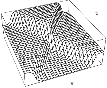
Figure 1: The interaction of a sine-Gordon soliton with an antisoliton.

The affine Toda equations of motion possess soliton solutions [26, 33]. These are kink configurations which interpolate between the different vacua of the Toda potential. The characteristic property of solitons is that they propagate without dispersion and that even after collision with other solitons they regain their original shape. As an example figure 1 shows a solution of the sine-Gordon model which describes an antisoliton and a soliton moving in opposite directions. One sees how they move through each other, the only effect of their interaction being a time delay.

These solitons can be quantized and then their scattering is described by factorizable S-matrices obeying the axioms of crossing symmetry, unitarity, Yang-Baxter equation and the bootstrap principle [36]. These S-matrices can be obtained by exploiting the affine quantum group symmetry of affine Toda theory [1].

Interestingly, certain of the classical multi-soliton solutions of affine Toda theory seem to make physical sense also if one views them only on the left half-plane. To illustrate this we have taken the solution of figure 1 and have restricted it to $x<0$ to arrive at figure 2. Now it describes a reflection process off a boundary at $x=0$ . The right-moving antisoliton hits the wall at $x=0$ and is reflected back as a soliton with opposite velocity.

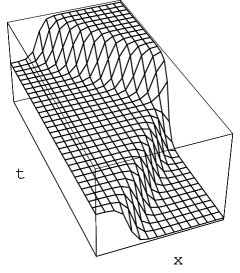
Figure 2: The solution of figure 1 interpreted as describing the elastic reflection of an antisoliton off a boundary at $x=0$.

In this paper we will investigate this possibility of restricting affine Toda theory to the left half-line by putting a reflecting boundary at $x=0$. In other words we will impose boundary conditions at $x=0$ which among all multi-soliton solutions of Toda theory on the whole line select only those which, when viewed on the left half-line, describe the purely elastic reflection of solitons off the boundary.

The existence of these classical solutions describing solitons on the half line opens up the challenge of deriving the corresponding quantum theory. In addition to the S-matrix describing the scattering of the solitons among themselves one will also have to construct a reflection matrix describing the reflection of the solitons off the boundary. The complete set of axioms which such reflection matrices have to satisfy was given by Ghoshal and Zamolodchikov [22] extending the early work of Cherednik [6]. Gandenberger [21] has found solutions to these axioms for the case of $a_{2}^{(1)}$ Toda theory.

In this paper we will prepare the ground for extending these investigations into the quantum theory of solitons on the half-line by performing classical and semiclassical calculations. By using the method of images we are able to complement the investigations which have already been performed on this subject. Corrigan et.al. [2] have classified boundary conditions which preserve integrability. We see that many of them descend from just the three boundary conditions which we study. The Durham group and in particular Bowcock [4] have studied the classical solutions of real coupling Toda theory on the half-line. There are conjectures for particle reflection matrices for real coupling Toda theory on the half-line [17, 35, 30]. In order to check these conjectures and to connect them with specific boundary conditions it is necessary to determine the classical vacuum solution [7]. Our analysis simplifies these calculations. Gandenberger [21] has determined quantum soliton reflection matrices by solving the boundary Yang-Baxter equation. We verify his results semiclassically by comparing with the time delays computed from our solutions. The idea of obtaining soliton solutions on the half-line from those on the whole line is of course not new. It has been applied to the sine-Gordon model in [34], to Toda lattice models in [19] and to real coupling Toda theory [4].

There is one affine Toda theory $T(\hat{g})$ for every affine simple complex Lie algebra $\hat{g}$. It describes an $n$-component bosonic field $\boldsymbol{\phi}$, where $n$ is the rank of $\hat{g}$. Let $\boldsymbol{\alpha}_{i},\,i=1,\dots,n$ be the simple roots of the finite-dimensional Lie algebra $g$ underlying $\hat{g}$ and let $\boldsymbol{\alpha}_{0}=-\sum_{i=1}^{n}\eta_{i}\boldsymbol{\alpha}_{i}$ be the extra simple root that needs to be added to obtain the extended Dynkin diagram of $\hat{g}$. Define $\eta_{0}=1$. Then the corresponding affine Toda theory $T(\hat{g})$ is described by the equations of motion

$$\ddot{\boldsymbol{\phi}}-\boldsymbol{\phi}^{\prime\prime}+m^{2}\sum_{i=0}^{n}\eta_{i}\boldsymbol{\alpha}_{i}e^{\boldsymbol{\alpha}_{i}\cdot\boldsymbol{\phi}}=0.$$ (1)

We have normalized the field so that the coupling constant does not appear in the equations of motion. We will use units where $m=c=1$. The sine-Gordon model is obtained by choosing $\hat{g}=a_{1}^{(1)}=\widehat{sl(2)}$.

This first section will explain our general ideas without going into calculational detail. Many of the arguments presented here apply to any affine Toda theory. In later sections we will do the calculations for the case of $a_{n}^{(1)}$ Toda theory. Section 2 reviews the solutions to $a_{n}^{(1)}$ Toda equations of motion in the Hirota formalism. In section 3 we will impose three different boundary conditions and identify the solutions of the equations of motion which satisfy these. We will use the results obtained to learn about real coupling Toda theory on the half-line in section 4 and to perform semiclassical checks of conjectured quantum reflection matrices in section 5. Section 6 contains discussions.

1.1 Neumann boundary condition

Figure 3: Space-time diagram for the soliton-antisoliton process satisfying the Neumann boundary condition.

One boundary condition which selects solutions of the form discussed above among all the multi-soliton solutions is the Neumann condition

$$\partial_{x}\boldsymbol{\phi}=0~{}~{}~{}\mbox{ at }~{}~{}x=0.$$ (2)

It is clear that any solution which is invariant under parity reversal $x\rightarrow-x$ will satisfy this boundary condition. Thus any solution composed of any number of soliton-antisoliton pairs with exactly equal but opposite velocities will satisfy the boundary condition provided the center of mass of each pair is at $x=0$. It is also easy to convince oneself that there are no other solutions which satisfy eq.(2). The solution plotted in figure 1 is an example of such a configuration with one soliton-antisoliton pair.

Figure 3 is a space-time diagram showing the worldlines of the centers of mass of the solitons in such a solution satisfying the Neumann boundary condition. Of course close to the interaction point the solitons loose their individual existence, thus the worldlines drawn in the figure are meant for illustrative purposes only. The fat solid lines are the trajectories of the two solitons on the whole line. The dotted lines are their asymptotic trajectories. The fine line will be explained below

The fact that the incoming and outgoing asymptotic trajectories do not meet the time axis at the same point indicates that the solitons experience a time delay during their interaction. We notice from the diagram that the time delay is negative, it is really a time advance. The fact that the solitons on the whole line are experiencing a time advance while they pass through each other shows that they are attractive to each other.

As a consequence of this time advance in soliton-antisoliton scattering also the reflected soliton on the half-line experiences a time advance during its interaction with the boundary. There are two possible interpretations for this time advance. One can imagine that the boundary is attractive and that the reflected soliton is reaching the boundary along the fat trajectory in figure 3. The soliton is accelerated by the attractive boundary while it is approaching and that is the reason for the time advance. Alternatively one can imagine that the boundary is repulsive and that the reflected soliton is moving along the fine trajectory in figure 3. Because it is repelled by the boundary the soliton already turns around some time before it actually reaches $x=0$ and this is the cause of the time advance. For reasons which we will explain we believe the boundary to be attractive and thus prefer the first interpretation.

In $a_{n}^{(1)}$ Toda theory there are $n$ types of solitons with masses

$$M_{a}=\frac{2(n+1)}{(i\beta)^{2}}m_{a}\text{~{}~{}~{}with~{}~{}~{}}m_{a}=2\sin\frac{a\pi}{n+1},~{}~{}a=1,\cdots,n.$$ (3)

The time delay which solitons of type $a$ experience during reflection is given by (see eq.(61))

$$\Delta t=\frac{\sqrt{1-v^{2}}}{m_{a}v}\log\left(1-\frac{m_{a}^{2}}{4}(1-v^{2})\right).$$ (4)

$\Delta t$ is always negative and its magnitude increases with the mass of the soliton while decreasing with its velocity. Thus light and fast solitons are affected less by the boundary than heavy and slow ones.

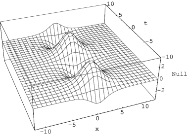
Figure 4: A breather solution

One can allow the relative rapidities between solitons to be complex (as long as one ensures that the corresponding solution does not develop singularities [24]). A configuration of two solitons whose relative rapidity is imaginary and which therefore are oscillating around each other in a bound state is called a breather, see figure 4. (If the breather has non-vanishing topological charge some authors call it ”breathing soliton” or ”excited soliton”).

Again one can describe breathers on the half-line by restricting a solution describing breather-antibreather pairs on the whole line. Thus we see that the spectrum of affine Toda theory on the half-line with a Neumann boundary condition is as rich as that on the whole line, consisting of any combination of solitons and breathers.

But Toda theory on the half-line contains even some new states not present in the spectrum on the whole line. These are boundary states. Consider a stationary breather as in figure 4 on the whole line centered at $x=0$. On the half-line this will be interpreted as a soliton bound to the boundary. We will call these configurations boundary breathers. The fact that the boundary can bind a soliton is the reason why we interpret it as an attractive boundary.

1.2 Other boundary conditions

In this paper we also study more general boundary conditions of the form

$$\partial_{x}\boldsymbol{\phi}|_{x=0}=\varepsilon\sum_{i=0}^{n}\ \eta_{i}\,\boldsymbol{\alpha}_{i}\ e^{\boldsymbol{\alpha}_{i}\cdot\boldsymbol{\phi}/2}|_{x=0}$$ (5)

$\varepsilon=0$ corresponds to the Neumann condition already discussed.

It is easy to see that a configuration describing a soliton and an antisoliton with opposite velocities on the whole line will satisfy the boundary conditions eq.(5) in the far past and in the far future by the following consideration.

At $t=-\infty$ the solitons are located at $x=-\infty$ and $x=\infty$ respectively and thus at $x=0$ the field takes the right asymptotic value of the right-moving soliton. The asymptotic values of a finite-energy solution of affine Toda theory must always be equal to a vacuum value of the Toda potential and are therefore of the form $2\pi i\boldsymbol{\lambda}$ where $\boldsymbol{\lambda}$ is some coweight of the underlying Lie algebra $g$. The difference between the left asymptotic value and the right asymptotic value (divided by $2\pi i$) is called the topological charge of the solution. Only the difference between the left and right asymptotic values is of physical relevance because the constant shift $\boldsymbol{\phi}\rightarrow\boldsymbol{\phi}+2\pi i\boldsymbol{\lambda}$ is a symmetry of affine Toda theory for any coweight $\boldsymbol{\lambda}$ and can be used to shift the asymptotic value at both ends simultaneously without changing the physics. It follows that we can always shift the soliton-antisoliton pair solution so that in the far past it takes the constant value $\boldsymbol{\phi}=0$ near $x=0$. It then satisfies the boundary condition eq.(5) because $\sum_{i=0}^{n}\eta_{i}\boldsymbol{\alpha}_{i}=0$.

At $t=\infty$ the solitons will have passed through each other and will again be infinitely separated. The value of the field at $x=0$ will be equal to $2\pi i(\boldsymbol{\lambda}_{2}-\boldsymbol{\lambda}_{1})$ where $\boldsymbol{\lambda}_{1}$ and $\boldsymbol{\lambda}_{2}$ are the topological charges of the right-moving and the left-moving solitons respectively. This satisfies the boundary condition if $\boldsymbol{\lambda}_{1}=\pm\boldsymbol{\lambda}_{2}$, i.e., if the two solitons are identical or if they are antiparticles of each other.

Figure 5: Reflection off the attractive boundary ($\varepsilon=-1)$.

What is less easy to see is under what circumstances these solutions satisfy the boundary conditions also at intermediate times. This requires detailed calculations which we will perform for $a_{n}^{(1)}$ Toda theory in section 3. We will find that a soliton-antisoliton pair can indeed satisfy the boundary conditions (5) if

$$\varepsilon^{2}=\frac{2}{|\boldsymbol{\alpha}_{i}|^{2}}.$$ (6)

We will choose the normalization of the roots so that $|\boldsymbol{\alpha}|^{2}=2$ and thus we need $\varepsilon=\pm 1$. Furthermore, in order to satisfy the boundary condition (5) the soliton and antisoliton must meet not at the boundary but either behind or in front of it. This is depicted in figures 5 and 6. In these figures the thin lines are the worldlines of the soliton and antisoliton on the whole line, the fat line is the worldline of the reflected soliton on the left half-line and the dotted lines are the asymptotic trajectories of the reflected soliton. The calculations in section 3 also show that there are no other two-soliton solutions on the whole line which satisfy the boundary conditions. Thus we see that a soliton on the half-line will always be converted into its antisoliton upon reflection from the boundary.

The distance $d(v)$ between the boundary and the center of mass of the soliton-antisoliton pair comes out of the calculation as

$$d(v)=\frac{-\varepsilon\sqrt{1-v^{2}}}{2m_{a}}\log\left(\frac{1+\frac{m_{a}}{2}\sqrt{1-v^{2}}}{1-\frac{m_{a}}{2}\sqrt{1-v^{2}}}\right).$$ (7)

We see that for $\varepsilon=-1$ the scattering with the mirror soliton takes place behind the boundary and for $\varepsilon=1$ it takes place in front of the boundary. The distance between the boundary and the virtual scattering point is smaller if the soliton is faster or lighter.

Figure 6: Reflection off the repulsive boundary ($\varepsilon=1)$.

The time delay which the soliton experiences during reflection is given by (see eq.(61))

$$\Delta t=\frac{2\sqrt{1-v^{2}}}{m_{a}v}\log\left(1-\varepsilon\frac{m_{a}}{2}\sqrt{1-v^{2}}\right).$$ (8)

It is negative for the $\varepsilon=1$ boundary and positive for the $\varepsilon=-1$ boundary.

The energy of a soliton in the presence of an $\varepsilon=-1$ boundary is less than the energy of a soliton on the whole line. Conversely the energy of a soliton in the presence of an $\varepsilon=1$ boundary is higher than on the whole line. Therefore we believe that the $\varepsilon=-1$ boundary should be called attractive and the $\varepsilon=1$ boundary should be called repulsive.

As we will see in section 3.6, the $\varepsilon=-1$ boundary permits boundary breather solutions which are regular for all $x<0$ and which have a finite energy on the half-line. However they have a singularity exactly at $x=0$. We are not sure whether they have a physical interpretation or not. The $\varepsilon=1$ boundary on the other hand does not allow any boundary breather solutions on the left half-line. This again confirms the identification of the $\varepsilon=1$ boundary as repulsive and the $\varepsilon=-1$ boundary as attractive.

The time advance which the soliton experiences during its reflection off the $\varepsilon=1$ boundary must be due to the fact that the soliton turns around before it reaches the boundary as indicated by the fat trajectory in figure 6. Note the curious fact that in the case of the Neumann boundary condition the soliton is also experiencing a time advance but in that case it is due to not to an early turnaround but it is due to the acceleration by the attractive boundary. This is reminiscent of a similarly confusing situation in sine-Gordon theory on the whole line. There the time advance during soliton-soliton scattering is interpreted as being due to a repulsive force between the solitons (the solitons reflect of each other before they reach each other) whereas the same time advance during soliton-antisoliton scattering is interpreted as being due to an attractive force between them (they accelerate while they move towards each other).

Another peculiarity is that while the boundary seems to either attract or repel moving solitons, it does not affect stationary solitons. All the three boundary conditions which we have studied allow stationary solitons to sit at an arbitrary distance from the boundary without being pulled into it or being pushed away. This is just like solitons which attract other solitons only when they are moving relative to each other.

While affine Toda theory in the bulk is invariant under the shift symmetry $\boldsymbol{\phi}\rightarrow\boldsymbol{\phi}+2\pi i\boldsymbol{\lambda}$, this is not true of the boundary. If we act with the shift symmetry on the boundary conditions (5) we obtain new boundary conditions

$$\partial_{x}\boldsymbol{\phi}|_{x=0}=\sum_{i=0}^{n}\ A_{i}^{(\boldsymbol{\lambda})}\,\eta_{i}\,\boldsymbol{\alpha}_{i}\ e^{\boldsymbol{\alpha}_{i}\cdot\boldsymbol{\phi}/2}|_{x=0},$$ (9)

with

$$A_{i}^{(\boldsymbol{\lambda})}=\varepsilon\,e^{i\pi\boldsymbol{\alpha}_{i}\cdot\boldsymbol{\lambda}}=\pm\varepsilon.$$ (10)

This fact that different boundary conditions are related by imaginary translations of the fields by weights was noted in [9]. These new boundary conditions are physically equivalent to the old ones because the solutions which satisfy these boundary conditions are obtained from those satisfying the old ones by a shift symmetry. We can therefore without loss of generality concentrate on just the three boundary conditions (5). The situation will be different in real coupling Toda theory which does not have the shift symmetry. This will be discussed below in section 1.3.

If the Coxeter number $h=\sum_{i=0}^{n}\eta_{i}$ is even (this is the case for example for $\hat{g}=c_{n}^{(1)}$ and $\hat{g}=a_{2m-1}^{(1)}$) the two boundary conditions (5) with $\varepsilon=1$ and $\varepsilon=-1$ are equivalent. They transform into each other under the shift $\boldsymbol{\phi}\rightarrow\boldsymbol{\phi}+2\pi i{\mathbf{\rho}}$ where $\mathbf{\rho}$ is the sum of the fundamental coweights. Thus there is no one-to-one correspondence between boundary conditions and boundaries. If $h$ is even then one and the same boundary condition allows both the attractive and the repulsive boundary. Indeed, having a solution describing reflection of the attractive boundary one can parity transform it ($x\rightarrow-x$) and shift it by $2\pi i\rho$ and one will obtain another solution satisfying the same boundary condition but now describing reflection off the repulsive boundary.

Affine Toda theory possesses an infinite number of conserved charges. These charges are higher-spin generalizations of energy and momentum and generate velocity-dependent time- and space translation symmetries. Corrigan et.al. [2] showed that boundary conditions of the form

$$\partial_{x}\boldsymbol{\phi}|_{x=0}=\sum_{i=0}^{n}\ A_{i}\,\sqrt{\frac{2\eta_{i}}{|\boldsymbol{\alpha}_{i}|^{2}}}\,\boldsymbol{\alpha}_{i}\ e^{\boldsymbol{\alpha}_{i}\cdot\boldsymbol{\phi}/2}|_{x=0},$$ (11)

preserve the velocity-dependent time translation symmetries if the coefficients $A_{i}$ satisfy some severe constraints. For simply laced algebras $\hat{g}$ the $A_{i}$ either have to all be zero (Neumann boundary condition) or they all have to satisfy $A_{i}^{2}=1$. These possibilities also exist for the non-simply laced algebras but the conditions are weaker and some coefficients can be allowed to take on arbitrary values.

Comparing the integrable boundary conditions (11) of Corrigan et.al with the boundary conditions (9) we notice a discrepancy. The boundary conditions (11) of Corrigan et.al. are generically not satisfied by the soliton-antisoliton pairs which we have discussed because $\sum_{i=0}^{n}\sqrt{2\eta_{i}/|\boldsymbol{\alpha}_{i}|^{2}}\boldsymbol{\alpha}_{i}$ is generally not zero. One will probably have to also include one or more stationary solitons near the boundary to soak up the discrepancy. How this works in general we have not yet investigated satisfactorily.

For $\hat{g}=a_{n}^{(1)}$ however all Kac labels $\eta_{i}$ are unity and all roots square to $2$ and thus our boundary conditions are integrable according to Corrigan et.al. In fact, if $n$ is even our boundary conditions eq.(9) exhaust all the integrable boundary conditions. If $n$ is odd, the coefficients $A_{i}^{(\boldsymbol{\lambda})}$ in our boundary conditions satisfy the constraint $\prod_{i=0}^{n}A_{i}^{(\boldsymbol{\lambda})}=1$ (because $\sum_{n=0}^{n}\boldsymbol{\alpha}_{i}=0$). In that case we are thus dealing with only half of all the possible integrable boundary conditions.

Also for $\hat{g}=c_{n}^{(1)}$ the integrable boundary conditions (11) reduce to the boundary conditions (9) because in that case $2/|\boldsymbol{\alpha}_{i}|^{2}=\eta_{i}$. Thus our method of images applies also to this case. As was explained in [5], the affine Toda theories for nonsimply-laced algebras can be obtained from those for simply-laced algebras by folding. In [13] it was explained how to apply this folding trick to obtain the soliton solutions of $c_{n}^{(1)}$ Toda theory from those of $a_{2n-1}^{(1)}$ Toda theory. Using this method, the calculations which we perform for the case of $a_{n}^{(1)}$ can be directly applied to the case of $c_{n}^{(1)}$.

Once one has shown that the single soliton-antisoliton pair satisfies an integrable boundary condition (possibly with some additional stationary solitons near the boundary in the case of $\hat{g}\neq a_{n}^{(1)}$) then one can deduce that a configuration describing any number of such pairs also satisfies them. The argument goes as follows:

Figure 7: a) Part of a multisoliton solution describing reflection off the attractive boundary in which the individual reflection processes are separated in time. b) This multisoliton configuration in which the two reflection processes are superposed is obtained from the solution in a) by a higher spin time translation symmetry. Thus it too is a solution satisfying the boundary condition.

If we have a configuration with several soliton-antisoliton pairs with real, nonzero and pairwise different velocities then we can use the velocity-dependent time translation symmetry transformations to separate the soliton pairs arbitrarily far so that at any time no more than one pair is close to the boundary. Thus the problem of showing that the configuration with many soliton-antisoliton pairs satisfies the boundary condition is reduced to showing that each pair individually does so. This is illustrated in figure 7. Configurations to which this argument doesn’t apply directly because some velocities are zero or complex can be viewed as limits or analytic continuations of the generic situation.

1.3 Real-coupling Toda theory

We have so far discussed the solutions to the Toda equations of motion and the boundary conditions under the assumption that the field $\boldsymbol{\phi}$ takes complex values. However the energy functional corresponding to the Toda equations of motion on the whole line is

$$E[\boldsymbol{\phi}]=\frac{1}{\beta^{2}}\int\limits_{-\infty}^{\infty}dx\left(\frac{1}{2}\dot{\boldsymbol{\phi}}^{2}+\frac{1}{2}\boldsymbol{\phi}^{\prime}{}^{2}+\sum_{i=0}^{n}\eta_{i}\left(e^{\boldsymbol{\alpha}_{i}\cdot\boldsymbol{\phi}}-1\right)\right),$$ (13)

where $\beta$ is an arbitrary normalization constant. For $\boldsymbol{\phi}$ complex, this energy functional is complex and neither its real nor its imaginary part are bounded from below. It would thus be very difficult to make sense of the corresponding quantum theory. Therefore before we can quantize affine Toda theory we have to restrict the allowed values for $\boldsymbol{\phi}$.

The simplest possibility is to let $\boldsymbol{\phi}$ and $\beta$ be real. Then the energy is manifestly positive definite and quantization is straightforward. This leads to the so-called real coupling Toda theories. Another much less straightforward possibility is called imaginary coupling Toda theory and consists in restricting $\boldsymbol{\phi}$ and $\beta$ to be purely imaginary, i.e., one lets $\tilde{\boldsymbol{\phi}}=-i\boldsymbol{\phi}$ and $\tilde{\beta}=-i\beta$ be real.

When one restricts to real fields none of the soliton or breather solutions survive (except in the case of sine-Gordon, which we do not treat). Indeed there is only one nonsingular classical solution which is real. It is the trivial solution $\boldsymbol{\phi}=0$. This is the vacuum around which one can then quantize the theory. The particles are the small fluctuations around this vacuum. Their scattering matrices have been determined exactly [5, 12].

Two interesting things happen once one restricts to the half-line. First of all, while there are no nontrivial real solutions to the affine Toda equations which are nonsingular on the whole line, there may be real solutions whose singularities all lie on the right half- line, out of harms way. Secondly the shift symmetry transformation $\boldsymbol{\phi}\rightarrow\boldsymbol{\phi}+2\pi i\boldsymbol{\lambda}$ is no longer allowed because it would map to a complex field. Therefore the boundary conditions in eq.(9) are no longer equivalent. Instead each choice of the signs $A_{i}$ defines a different real coupling Toda theory on the half-line.

The task therefore arises to find for each boundary condition those real solutions which are nonsingular on the left half-line. This is particularly important because the trivial vacuum solution $\boldsymbol{\phi}=0$ does not satisfy most of these boundary conditions and an alternative vacuum solution must be found before one can start to quantize these theories.

This problem has been addressed already by Bowcock in [4] for $a_{n}^{(1)}$ Toda theory on the half-line. We repeat his analysis in section 4 in our formalism. We find that if one puts a single stationary soliton (and its mirror antisoliton) at just the right distance (given by eq.(80)) from the $\varepsilon=-1$ boundary and adds a constant $2\pi i\boldsymbol{\lambda}$ where $\boldsymbol{\lambda}$ is the topological charge of the soliton one obtains a real nonsingular solution. One obtains the identical solution if one replaces $\boldsymbol{\lambda}$ by $-\boldsymbol{\lambda}$ because soliton and antisoliton enter symmetrically in the solution.

While we can not prove it, we believe that this is the only nonsingular real solution. No nonsingular real solutions can be obtained from the solutions for the $\varepsilon=1$ boundary.

In the approach of [4] it was not so easy to determine which particular boundary conditions the real solutions satisfy. For us this is trivial because we can view the stationary real soliton as the limit of a moving complex soliton as the velocity goes to zero. For a moving soliton one can perform the analysis at a time when the soliton is far away. At the boundary the field then takes the constant value $\boldsymbol{\phi}=2i\pi\boldsymbol{\lambda}$. It therefore satisfies the boundary condition

$$\partial_{x}\boldsymbol{\phi}|_{x=0}=\sum_{i=0}^{n}\ A_{i}^{(\boldsymbol{\lambda})}\,\eta_{i}\,\boldsymbol{\alpha}_{i}\ e^{\boldsymbol{\alpha}_{i}\cdot\boldsymbol{\phi}/2}|_{x=0},$$ (14)

with

$$A_{i}^{(\boldsymbol{\lambda})}=-e^{i\pi\boldsymbol{\alpha}_{i}\cdot\boldsymbol{\lambda}}.$$ (15)

Because the different boundary conditions are not continuously connected, the boundary condition satisfied by the solution can not change as the velocity is taken to zero. Thus also the real stationary soliton solution satisfies this boundary condition.

The topological charges $\boldsymbol{\lambda}$ of single solitons in $a_{n}^{(1)}$ Toda theory are known to be weights in the fundamental representations of $a_{n}$. As $\boldsymbol{\lambda}$ runs through all the weights in the fundamental representations $A_{i}^{(\boldsymbol{\lambda})}$ runs through all possible sign combinations with the property that

$$\prod_{i=0}^{n}A_{i}^{(\boldsymbol{\lambda})}=(-1)^{n+1},$$ (16)

except for the one with $\boldsymbol{\lambda}=0$ which corresponds to the trivial solution $\boldsymbol{\phi}=0$. This implies that if all the weights in the fundamental representation were realized as topological charges of solitons, then we would have found a vacuum solution for every real coupling $a_{n}^{(1)}$ Toda theory with a boundary condition which satisfies the constraint (16). Furthermore every sign combination is obtained exactly twice as $A_{i}^{(\boldsymbol{\lambda})}=A_{i}^{(-\boldsymbol{\lambda})}$. These two correspond to the same solution however and thus we find exactly one vacuum solution to every boundary condition.

However not for every weight in the fundamental representations has a classical soliton solution been found which has this weight as its topological charge. This has been a puzzle because in the quantum theory of imaginary coupling Toda theory the solitons need to fill out the entire representations. This puzzle has often been interpreted as an indication that imaginary coupling Toda theory is sick. Now however it is hitting us even in real coupling Toda theory. If solitons exist for all weights in the fundamental representations then we get a vacuum solution for all boundary conditions of the form (14) with the constraint (16). If solitons do not exist for all weights, then some of those boundary conditions don’t have a vacuum. This seems a bit unnatural. It seems that the semiclassical analysis, which is used to make the correspondence between classical solutions and quantum states is breaking down. It is my belief that the same, as yet unknown, mechanism which provides the missing quantum soliton states in the imaginary coupling Toda theory will also provide the missing quantum vacuum states in the real coupling Toda theory on the half-line with the boundary conditions satisfying the constraint (16).

Even more dubious is the situation for those real coupling Toda theories on the half-line for which the boundary conditions do not satisfy (16). For these we don’t find any vacuum solutions even if we work with the full set of solitons. We thus seem to have no handle on the quantum theory for these. This agrees with an observation made by Corrigan et.al. during their work on [9]. They tried to derive the classical reflection factor for $a_{2}^{(1)}$ with boundary condition specified by $A_{0}=A_{1}=-1$ and $A_{2}=1$ which does not satisfy the condition (16) and found a bizzare-looking result [private communication].

There is another puzzling fact about the classical soliton solutions of affine Toda theory which now finds its way into real coupling Toda theory. The classical soliton solution contains a certain angular parameter $\zeta$ which can take on any value between $0$ and $2\pi$. This is the parameter which determines the asymptotic value of the solution and thus the topological charge of the soliton. However there is only a discrete set of topological charges. The way this works is that the interval $[0,2\pi]$ is split into several intervals. The topological charge stays constant for $\zeta$ within one of these intervals and changes discontinuously as $\zeta$ crosses into the next interval. Thus there is actually a family of solutions for each soliton with a specific topological charge, parametrized by a continuous parameter ranging over an interval. It is not well understood in the semiclassical approximation what the effect of such a restricted zero-mode is. But because there are so many things in the semiclassical approximation for imaginary coupling Toda theory which are not well understood, not much attention has been paid to this particular problem.

Figure 8: Plot of the vacuum solution of $a_{2}^{(1)}$ Toda theory with $A_{0}=-1,A_{1}=A_{2}=1$ at two different values of the modulus parameter $\zeta$. The left plot is at $\zeta=0$, the right plot is at $\zeta=0.5$.

Now the same continuous parameter appears in the vacuum solutions of real coupling Toda theory with a boundary. To give an idea of what these vacuum solutions look like, we have plotted the vacuum solution for $a_{2}^{(1)}$ affine Toda theory with the boundary condition specified by $A_{0}=-1$, $A_{1}=A_{2}=1$ in figure 8 for two different values of the parameter $\zeta$. The field $\boldsymbol{\phi}$ of $a_{2}^{(1)}$ Toda theory is a two-component vector. We have plotted $\phi_{1}=\boldsymbol{\lambda}_{1}\cdot\boldsymbol{\phi}$ with a solid line and $\phi_{2}=\boldsymbol{\lambda}_{2}\cdot\boldsymbol{\phi}$ with a dashed line. For $\zeta=0$ the two components coincide and both have a singularity on the right half-line. For $\zeta=0.5$ the component $\phi_{2}$ is no longer singular. Any value of $\zeta$ between $-\pi/6$ and $\pi/6$ gives a different solution to these boundary conditions, all with the same energy. It will be interesting to study what, if any, consequences this vacuum degeneracy has for the quantum theory.

This concludes our general discussion and we now turn to concrete calculations.

2 Review of classical solutions on the whole line

This section reviews well known facts about the classical solutions of affine Toda theory which we will use.

2.1 Hirota’s tau functions

Applying a method developed by Hirota [25] and adapted to affine Toda theories by Hollowood [26], one parameterizes the $n$-component field $\boldsymbol{\phi}$ by the $n+1$ tau functions $\tau_{i}$ as

$$\boldsymbol{\phi}(x)-\boldsymbol{\phi}(-\infty)=-\sum_{i=0}^{n}\frac{2\boldsymbol{\alpha}_{i}}{\boldsymbol{\alpha}_{i}^{2}}\,\ln\tau_{i}.$$ (17)

For finite energy solutions $\boldsymbol{\phi}(-\infty)$ will have to lie in one of the minima of the Toda potential, i.e., $\boldsymbol{\phi}(-\infty)=2\pi i\boldsymbol{\lambda}$ where $\boldsymbol{\lambda}$ can be any coweight of the underlying finite dimensional Lie algebra $g$. Which minima is chosen is irrelevant because the constant shift $\boldsymbol{\phi}\rightarrow\boldsymbol{\phi}+2\pi i\boldsymbol{\lambda}$ is a symmetry of affine Toda theory for any coweight $\boldsymbol{\lambda}$.

Substituting the parameterization (17) into the equations of motion (1) gives

$$\sum_{i=0}^{n}\,\boldsymbol{\alpha}_{i}\,\frac{1}{\tau_{i}^{2}}\,\left(\frac{2}{\boldsymbol{\alpha}_{i}^{2}}\left(\ddot{\tau_{i}}\tau_{i}-\dot{\tau}_{i}^{2}-\tau_{i}^{\prime\prime}\tau_{i}+{\tau^{\prime}}_{i}^{2}\right)-\eta_{i}\prod_{j=0}^{n}\,\tau_{j}^{I_{ij}}\right)=0,$$ (18)

where $I_{ij}$ is the incidence matrix $I_{ij}=-2\boldsymbol{\alpha}_{i}\cdot\boldsymbol{\alpha}_{j}/\boldsymbol{\alpha}_{j}^{2}+2\delta_{ij}$. Having introduced $n+1$ tau functions we can choose one of them to satisfy the equation

$$\ddot{\tau_{0}}\tau_{0}-\dot{\tau_{0}}^{2}-\tau_{0}^{\prime\prime}\tau_{0}+{\tau^{\prime}}_{0}^{2}=\frac{\boldsymbol{\alpha}_{0}^{2}}{2}\left(\prod_{j=0}^{n}\,\tau_{j}^{I_{0j}}-\tau_{0}^{2}\right)$$ (19)

Multiplying eq. (18) by fundamental weights $\boldsymbol{\lambda}_{i}$ and using eq. (19) one obtains the following set of equations of motion

$$\ddot{\tau_{i}}\tau_{i}-\dot{\tau_{i}}^{2}-\tau_{i}^{\prime\prime}\tau_{i}+{\tau^{\prime}}_{i}^{2}=\frac{\boldsymbol{\alpha}_{i}^{2}}{2}\eta_{i}\left(\prod_{j=0}^{n}\,\tau_{j}^{I_{ij}}-\tau_{i}^{2}\right),~{}~{}~{}~{}i=1,\dots,n$$ (20)

which thus take the same form as eq. (19).

2.2 The soliton solutions for $a_{n}^{(1)}$

The parameterization of $\boldsymbol{\phi}$ in terms of Hirota $\tau$ functions turns out to be particularly useful in the case of $\hat{g}=a_{n}^{(1)}$ where the equations of motion (20) are quadratic in the $\tau$ once one substitutes the particular form of the incidence matrix $I_{ij}$.

$$\ddot{\tau_{i}}\tau_{i}-\dot{\tau_{i}}^{2}-\tau_{i}^{\prime\prime}\tau_{i}+{\tau^{\prime}}_{i}^{2}=\tau_{i-1}\tau_{i+1}-\tau_{i}^{2},~{}~{}~{}~{}i=0,\dots,n$$ (21)

We have defined $\tau_{-1}\equiv\tau_{n}$ and $\tau_{n+1}\equiv\tau_{0}$.

The single soliton solutions to these equations are

$$\tau_{j}^{(a)}=1+e^{\Omega}\omega^{ja},~{}~{}~{}~{}~{}~{}a=1,\dots,n$$ (22)

with

$$\Omega=\sigma(x-vt)-\xi,\qquad\qquad\omega=e^{\frac{2\pi i}{n+1}}$$ (23)

and

$$\sigma^{2}(1-v^{2})=4\sin^{2}\frac{a\pi}{n+1}\equiv m_{a}^{2}$$ (24)

Here $a=1,\dots,n$ labels the species of soliton, $v$ is the velocity, $1/\sigma$ the width of the soliton and relation (24) expresses the Lorentz contraction. We choose $\sigma$ positive. $\xi=\rho+i\zeta$ is an arbitrary complex number. Its real part $\rho$ determines the center of mass position, while its imaginary part $\zeta$ determines the asymptotic values of the soliton solution, and therefore its topological charge [26, 31]. For a fixed topological charge the parameter $\zeta$ can still range over an interval. The topological charge is defined as $(\boldsymbol{\phi}(\infty)-\boldsymbol{\phi}(-\infty))/2\pi i$ and turns out to always be a weight of the $a$th fundamental representation of $a_{n}$. The fact that the asymptotic values of $\boldsymbol{\phi}$ are purely imaginary means that these solutions will play a role only in the imaginary coupling Toda theory.

The Hirota Ansatz gives the multi-soliton solutions by a nonlinear superposition. For two solitons this takes the form

$$\tau_{j}=1+e^{\Omega_{1}}\omega^{ja_{1}}+e^{\Omega_{2}}\omega^{ja_{2}}+X_{12}e^{\Omega_{1}+\Omega_{2}}\omega^{j(a_{1}+a_{2})}$$ (25)

with the “interaction” function

$$X_{12}=-\frac{(\sigma_{1}-\sigma_{2})^{2}-(\sigma_{1}v_{1}-\sigma_{2}v_{2})^{2}-m^{2}_{a_{1}-a_{2}}}{(\sigma_{1}+\sigma_{2})^{2}-(\sigma_{1}v_{1}+\sigma_{2}v_{2})^{2}-m^{2}_{a_{1}+a_{2}}}.$$ (26)

It is sometimes useful to use the rapidity variables $\theta_{p}$ defined by $v_{p}=\tanh(\theta_{p})$. Then $\sigma_{p}=m_{a_{p}}\,\cosh(\theta_{p})$ and $\sigma_{p}\,v_{p}=m_{a_{p}}\,\sinh(\theta_{p})$. The interaction function $X_{pq}$ depends only on the relative rapidity $\theta=\theta_{p}-\theta_{q}$

$$X_{pq}(\theta)=\frac{\sinh\left(\frac{\theta}{2}+\frac{i\pi(a_{p}-a_{q})}{2n+2}\right)\sinh\left(\frac{\theta}{2}-\frac{i\pi(a_{p}-a_{q})}{2n+2}\right)}{\sinh\left(\frac{\theta}{2}+\frac{i\pi(a_{p}+a_{q})}{2n+2}\right)\sinh\left(\frac{\theta}{2}-\frac{i\pi(a_{p}+a_{q})}{2n+2}\right)}.$$ (27)

At the far past the two solitons described by the solution (25) are far apart and have their original shape. They then interact and deform at intermediate times and reemerge in the far future with their original shape regained but at shifted positions. We can determine the asymptotic trajectories of the right-moving soliton by taking the limits of the solution as $t\rightarrow\pm\infty$ while keeping $x-vt$ fixed

$$\lim_{\stackrel{{\scriptstyle t\rightarrow-\infty}}{{x-vt\text{ fixed}}}}\tau_{j} = 1+e^{\Omega_{1}}\omega^{ja_{1}},$$ (28)

$$\lim_{\stackrel{{\scriptstyle t\rightarrow\infty}}{{x-vt\text{ fixed}}}}\tau_{j} = \left(1+X_{12}e^{\Omega_{1}}\omega^{ja_{1}}\right)e^{\Omega_{2}}\omega^{ja_{2}}.$$ (29)

Similarly we can look at the left-moving soliton

$$\lim_{\stackrel{{\scriptstyle t\rightarrow-\infty}}{{x+vt\text{ fixed}}}}\tau_{j} = \left(1+X_{12}e^{\Omega_{2}}\omega^{ja_{2}}\right)e^{\Omega_{1}}\omega^{ja_{1}},$$ (30)

$$\lim_{\stackrel{{\scriptstyle t\rightarrow\infty}}{{x+vt\text{ fixed}}}}\tau_{j} = 1+e^{\Omega_{2}}\omega^{ja_{2}}.$$ (31)

We have plotted these trajectories for the case $\sigma_{1}=\sigma_{2}$ and $v_{1}=-v_{2}=v>0$ in figure 9.

Figure 9: Details of a two-soliton scattering process. For simplicity we plotted two solitons of equal mass in their center of mass frame. The thin lines are the asymptotic trajectories as read off from equations (28)-(31). The thick lines are fictitious interpolations between them. The drawing takes into account that $\log X$ is always negative.

We read off that asymptotically the only observable effect of the interaction between the two solitons is that they have experienced a time-delay $\Delta t$ given by

$$\Delta t=\frac{\log X_{12}}{\sigma v}.$$ (32)

This time delay is always negative (a time advance really) because $\log X_{12}$ is always negative [16].

The solitons satisfy a classical exclusion principle: one can not have two or more solitons of the same species traveling with the same velocity. If one tries to construct such a solution one finds that $X_{12}$ in eq. (26) vanishes and thus the $\tau_{j}$ in eq. (25) collapse to a one-soliton solution with a shifted position.

An $N$-soliton solution is given by

$$\tau_{j}=\sum_{\mu_{1}=0}^{1}\cdots\sum_{\mu_{N}=0}^{1}\prod_{p=1}^{N}\left(\left(\prod_{q=1}^{p-1}\left(X_{pq}\right)^{\mu_{q}}\right)e^{\Omega_{p}}\omega^{ja_{p}}\right)^{\mu_{p}}.$$ (33)

Let us again look at the asymptotic positions of the solitons. We choose the labeling so that $v_{1}\geq v_{2}\geq\cdots\geq v_{N}$. We then look at the $r$-th soliton by taking the limits $t\rightarrow\pm\infty$ while keeping $x-v_{r}t$ fixed. We assume for simplicity that there is no other soliton with velocity $v_{r}$. If there were such a soliton, it would have no effect on the position of the $r$-th soliton.

$$\lim_{t\rightarrow-\infty}\tau_{j} = \left(1+\prod_{p=1}^{r-1}X_{pr}e^{\Omega_{r}}\omega^{ja_{r}}\right)\prod_{p=1}^{r-1}\left(\prod_{q=1}^{p-1}X_{pq}\right)e^{\Omega_{p}}\omega^{ja_{p}},$$

$$\lim_{t\rightarrow\infty}\tau_{j} = \left(1+\prod_{p=r+1}^{N}X_{pr}e^{\Omega_{r}}\omega^{ja_{r}}\right)\prod_{p=r+1}^{N}\left(\prod_{q=p+1}^{N}X_{pq}\right)e^{\Omega_{p}}\omega^{ja_{p}}.$$ (34)

Thus we see that at $t=\infty$ the soliton is shifted with respect to the expected position by the amount

$$\sigma\,\Delta x=\sum_{p=1}^{r-1}\log X_{pr}-\sum_{r+1}^{N}\log X_{pr}.$$ (35)

Thus each time a soliton $p$ scatters with another soliton $q$ it is shifted by $\log X_{pq}$ if soliton $q$ comes from the left and it is shifted by the negative of $\log X_{pq}$ if it comes from the right. Because $\log X_{pq}$ is always negative [16] this can be interpreted as an attractive force between the solitons.

2.3 The energy in terms of tau functions

An expression for the energy in terms of the $\tau$ functions can be obtained by substituting eq. (17) into the energy functional (13), giving

$$E[\tau]=\frac{1}{\beta^{2}}\int\limits_{-\infty}^{\infty}dx\sum_{i=0}^{n}\left(\frac{1}{\boldsymbol{\alpha}_{i}^{2}}\sum_{j=0}^{n}a_{ij}\frac{\dot{\tau}_{i}\dot{\tau}_{j}+\tau_{i}^{\prime}\tau_{j}^{\prime}}{\tau_{i}\tau_{j}}+\eta_{i}\prod_{j=0}^{n}\tau_{j}^{-a_{ij}}-\eta_{i}\right),$$ (36)

where $a_{ij}=2\boldsymbol{\alpha}_{i}\cdot\boldsymbol{\alpha}_{j}/\boldsymbol{\alpha}_{j}^{2}$ is the Cartan matrix of $\hat{g}$.

In [32] it was observed that for soliton solutions the energy density could be rewritten as a total derivative so that the energy is given as a surface term, which in terms of $\tau$ functions is

$$E[\tau]=\left[-\frac{2}{\beta^{2}}\sum_{i=0}^{n}\frac{2}{\alpha_{i}^{2}}\frac{\tau_{i}^{\prime}}{\tau_{i}}\right]_{x=-\infty}^{\infty}.$$ (37)

Evaluating this for the soliton solutions of $a_{n}^{(1)}$ Toda theory in eq. (22) one gets

$$E_{\text{{\small soliton}}}=-\frac{2}{\beta^{2}}\sum_{i=0}^{n}\sigma=-\frac{2(n+1)}{\beta^{2}}\sigma.$$ (38)

This energy is real and positive for imaginary coupling constant $\beta=i\tilde{\beta}$. The rest mass of a soliton of type $a$ is thus[26]

$$M_{a}=\frac{2(n+1)}{\tilde{\beta}^{2}}\,m_{a}.$$ (39)

The energy of multi-soliton solutions is just the sum of the energy of the individual solitons [32].

3 Classical solutions on the half-line

Among the solutions of the equations of motion (20) reviewed in the previous section we will now identify those which satisfy the boundary conditions (5) at $x=0$. Except for the following first two general sections we will again restrict ourselves to $\hat{g}=a_{n}^{(1)}$. We will also not pay attention to the rather special case of $n=1$ (the sine-Gordon model) because this has been well studied already [34].

3.1 The boundary conditions

The Hirota formalism is extremely well suited for dealing with boundary conditions of the form (5) because they too lead to equations quadratic in the $\tau$. This has first been observed and exploited by Bowcock in [4].

Substituting the Hirota Ansatz (17) into the boundary condition (5) and taking the inner products with the fundamental weights $\boldsymbol{\lambda}_{i}$ leads to the set of $n+1$ equations

$$\frac{\tau_{i}^{\prime}}{\tau_{i}}+\varepsilon\,\eta_{i}\,\frac{\alpha_{i}^{2}}{2}\prod_{j=0}^{n}\tau_{j}^{-\frac{a_{ij}}{2}}=\eta_{i}\,C~{}~{}~{}~{}\text{at }x=0,~{}~{}~{}i=0,\dots,n,$$ (40)

where $C$ is some constant. Taking the square of eq. (40) and multiplying by $\tau_{i}^{2}$ gives

$$\varepsilon^{2}\,\prod_{j=0}^{n}\tau_{j}^{I_{ij}}=\left(\frac{2}{\alpha_{i}^{2}\eta_{i}}\right)^{2}\left(\eta_{i}C\tau_{i}-\tau_{i}^{\prime}\right)^{2}~{}~{}~{}~{}\text{at }x=0.$$ (41)

Upon specializing to $a_{n}^{(1)}$ Toda theory one obtains

$$\varepsilon^{2}\tau_{i-1}\tau_{i+1}-\left(C\tau_{i}-\tau_{i}^{\prime}\right)^{2}=0,~{}~{}~{}\;i=0,\dots n,$$ (42)

again valid only at $x=0$. We have defined $\tau_{-1}\equiv\tau_{n}$ and $\tau_{n+1}\equiv\tau_{0}$.

In addition to this condition on the tau functions the boundary condition also restricts the asymptotic value of the solution at $x=-\infty$. If the solution describes $m$ incoming solitons with topological charges $\boldsymbol{\lambda}_{k}$ then we need

$$\boldsymbol{\phi}(-\infty)=2\pi i\sum_{k=1}^{m}\boldsymbol{\lambda}_{k}\,+4\pi i\boldsymbol{\lambda},$$ (43)

where $\boldsymbol{\lambda}$ can be any coweight of $g$. As already explained in the introduction this ensures that at $t=-\infty$, when all solitons are infinitely far from the boundary, the field takes the constant value $4\pi i\boldsymbol{\lambda}$ at $x=0$ which satisfies the boundary condition. Because the full Lagrangian including the boundary potential is invariant under constant shifts $\boldsymbol{\phi}\rightarrow\boldsymbol{\phi}+4\pi i\boldsymbol{\lambda}$ for any coweight $\boldsymbol{\lambda}$, all configurations which differ only by such a shift are physically equivalent.

In affine Toda theory on the whole line two configurations which differ by $2\pi i\boldsymbol{\lambda}$ are equivalent. But on the half line, unless $\boldsymbol{\lambda}$ is equal to twice some other coweight, only one of these combinations can satisfy the boundary condition and the other one is projected out of the theory.

3.2 The energy

It was observed by Bowcock [4] that the constant $C$ occurring above is proportional to the energy of the solution. This is seen as follows. The energy functional for Toda theory on the half-line consists of a contribution from the bulk and a contribution from the boundary, $E[\boldsymbol{\phi}]=E_{\text{{\small bulk}}}[\boldsymbol{\phi}]+E_{\text{{\small boundary}}}[\boldsymbol{\phi}_{0}]$, where the bulk contribution is similar to eq. (13) or eq. (36) except that the integration runs only from $-\infty$ to $0$. The boundary contribution is

$$E_{\text{{\small boundary}}}[\boldsymbol{\phi}_{0}]=-\varepsilon\frac{2}{\beta^{2}}\sum_{i=0}^{n}\,\eta_{i}\,e^{\boldsymbol{\alpha}_{i}\cdot\boldsymbol{\phi}(0)/2}.$$ (44)

Again, for soliton solutions the bulk contribution is given by a surface term and, putting the two together, one has

$$E[\tau]=-\frac{2}{\beta^{2}}\sum_{i=0}^{n}\left[\frac{2}{\alpha_{i}^{2}}\frac{\tau_{i}^{\prime}}{\tau_{i}}+\varepsilon\,\eta_{i}\,e^{\boldsymbol{\alpha}_{i}\cdot\boldsymbol{\phi}/2}\right]^{x=0},$$ (45)

(the contribution from $x=-\infty$ is zero). Comparing this to eq. (40) one finds that

$$E=-\frac{2}{\beta^{2}}\tilde{h}\,C,~{}~{}~{}\text{where }\tilde{h}=\left(\sum_{i=0}^{n}\frac{2\eta_{i}}{\alpha_{i}^{2}}\right).$$ (46)

From here on we will specialize to $a_{n}^{(1)}$. Then $\tilde{h}=n+1$.

3.3 Restricting two-soliton solutions to the half-line

We will now look for two-soliton solutions which satisfy the boundary conditions (42) and which can thus be restricted to the half-line to describe the reflection of a single soliton off a boundary. It follows from integrability that the reflection of a soliton off the boundary has to be completely elastic. The mass and the velocity of the soliton have to be the same before and after the reflection. In terms of the two-soliton solution on the whole line this means that the right-moving and the left-moving solitons have to have the same but opposite velocities and have to lie in either the same or in conjugate representations. Such a two-soliton solution is given by eq. (25) with

$$\Omega_{1}=\sigma(x-vt)-\xi_{1},~{}~{}~{}~{}\Omega_{2}=\sigma(x+vt)-\xi_{2},$$ (47)

We first treat the case

$$a_{2}=n+1-a_{1},$$ (48)

i.e., the reflected soliton is in the conjugate representation. We introduce the abbreviations $a_{1}=a$, $X_{12}=X$ and $(\xi_{1}+\xi_{2})/2=\xi$ and find from eq. (25) that

$$\tau_{i}|_{x=0} = 1+Xe^{-2\xi}+\omega^{ia}e^{-\sigma vt-\xi_{1}}+\omega^{-ia}e^{\sigma vt-\xi_{2}},$$ (49)

$$\tau_{i}^{\prime}|_{x=0} = \sigma\left(2Xe^{-2\xi}+\omega^{ia}e^{-\sigma vt-\xi_{1}}+\omega^{-ia}e^{\sigma vt-\xi_{2}}\right).$$ (50)

Substituting these expressions into the boundary conditions (42) one obtains the equations

$$0\,=\,B_{0} + B_{1}\left(\omega^{ia}e^{-\sigma vt-\xi_{1}}+\omega^{-ia}e^{\sigma vt-\xi_{2}}\right)$$

$$+B_{2}\left(\omega^{2ia}e^{2(-\sigma vt-\xi_{1})}+\omega^{-2ia}e^{2(\sigma vt-\xi_{2})}\right),~{}~{}~{}~{}\forall i$$

where

$$B_{2} = \varepsilon^{2}-\left(C-\sigma\right)^{2},$$ (52)

$$B_{1} = \left(\varepsilon^{2}(\omega^{a}+\omega^{-a})-2C\left(C-\sigma\right)\right)$$ (53)

$$+e^{-2\xi}X\left(\varepsilon^{2}(\omega^{a}+\omega^{-a})-2\left(C-2\sigma\right)\left(C-\sigma\right)\right)$$

$$B_{0} = \allowbreak\left(\varepsilon^{2}-C^{2}\right)+e^{-2\xi}\left(\varepsilon^{2}(\omega^{2a}+\omega^{-2a})-2(C-\sigma)^{2}\right)$$

$$+2e^{-2\xi}X\left(\varepsilon^{2}-C^{2}+2\sigma C\right)$$

$$+e^{-4\xi}X^{2}\left(\varepsilon^{2}-C^{2}+4\sigma\left(C-\sigma\right)\right)$$

We can easily calculate the constant $C$ by making use of the fact that it is proportional to the energy and thus is time-independent. This allows us to choose to evaluate it at $t=-\infty$ where at $x=0$ we have $\tau_{i}^{\prime}/\tau_{i}=\sigma$ and $\boldsymbol{\phi}=0$ and thus

$$C=\sigma+\varepsilon.$$ (55)

Because the equations (3.3) have to hold for all times, all the $B_{p}$ have to be zero if $v\neq 0$. Even if $v=0$ the terms still have to vanish separately unless $\omega^{2a}=1$. We will deal with this case separately later. $B_{2}=0$ automatically because of eq.(55). The equation $B_{1}=0$ becomes

$$e^{2\xi}=X\frac{\left(1-\varepsilon\frac{m_{a}^{2}}{2\sigma}\right)}{\left(1+\varepsilon\frac{m_{a}^{2}}{2\sigma}\right)}$$ (56)

where we used that $\omega^{a}+\omega^{-a}-2=-m_{a}^{2}$ and that $m_{a}^{2}<2\sigma$ unless $a=(n+1)/2$ (the case $\omega^{2a}=1$). We are left with one more equation $B_{0}=0$ and no further parameters which could be adjusted. Luckily one finds that this equation is satisfied automatically.

Using that the expression (26) for $X$ simplifies to

$$X=\left(1+\frac{m_{a}^{2}}{2\sigma}\right)\left(1-\frac{m_{a}^{2}}{2\sigma}\right),$$ (57)

we find

$$e^{2\xi}=\left\{\begin{array}[]{l}\left(1-\varepsilon\,\frac{m_{a}^{2}}{2\sigma}\right)^{2}\text{for }\varepsilon=\pm 1\\ \left(1-\varepsilon\,\frac{m_{a}^{2}}{2\sigma}\right)\left(1+\varepsilon\,\frac{m_{a}^{2}}{2\sigma}\right)~{}~{}~{}\text{for }\varepsilon=0\end{array}\right.$$ (58)

This can be expressed in terms of the rapidity $\theta$ of the soliton by noting that

$$1\pm\frac{m_{a}^{2}}{2\sigma}=\frac{\cosh\theta\pm\sin\frac{a\pi}{n+1}}{\cosh\theta}.$$ (59)

From this expression it is immediately obvious that $1\pm\frac{m_{a}^{2}}{2\sigma}$ is always real and positive for real $\theta$ (real velocity) and therefore $\xi$ is real. However for imaginary $\theta$ (imaginary velocity), which will be relevant for breather solutions, $1-\frac{m_{a}^{2}}{2\sigma}$ can be negative and thus for $\varepsilon=0$ the imaginary part of $2\xi$ can be equal to $\pi$.

Figure 10: Diagram of the soliton-antisoliton solution. Depending on the value of $d=\xi_{1}+\xi_{2}-\log X$ the solution can describe the reflection of a soliton on the left half-line of three different boundaries. We have combined all three cases in this one diagram. The thick lines are the asymptotic trajectories of the reflected soliton. The time delay can be read of from the distance between the points at which these lines intersect the boundary.

The displacement $d$ of the center of mass of the two-soliton system is (see figure 10)

$$d=\frac{1}{2\sigma}\left(2\xi-\log X\right)=\frac{1}{2\sigma}\log\left(\frac{1-\varepsilon\frac{m_{a}^{2}}{2\sigma}}{1+\varepsilon\frac{m_{a}^{2}}{2\sigma}}\right).$$ (60)

Thus $\varepsilon$ determines whether the virtual scattering takes place behind the boundary $(\varepsilon=-1)$, exactly at the boundary $(\varepsilon=0)$, or in front of it $(\varepsilon=+1)$. This is the result for $d$ which was reported in the introduction in eq.(7).

The time-delay $\Delta t$ which the soliton on the half-line is experiencing at the boundary is given by $\Delta t=2\xi/\sigma v$ (see figure 10).

$$\Delta t=\left\{\begin{array}[]{l}\frac{2}{\sigma v}\log\left(1-\varepsilon\,\frac{m_{a}^{2}}{2\sigma}\right)~{}~{}~{}\text{for }\varepsilon=\pm 1\\ \frac{1}{\sigma v}\log\left(\left(1+\frac{m_{a}^{2}}{2\sigma}\right)\left(1-\frac{m_{a}^{2}}{2\sigma}\right)\right)~{}~{}~{}\text{for }\varepsilon=0\end{array}\right.$$ (61)

If we choose $a_{2}=a_{1}$ instead of eq.(48) and repeat the analysis, we find that this does not lead to solutions. Thus a soliton always turns into an antisoliton upon reflection from the boundary, it can never come back as a soliton.

The energy of the soliton on the left half-line plus the boundary is

$$E=\frac{2(n+1)}{\tilde{\beta}^{2}}\left(\sigma+\varepsilon)\right).$$ (62)

Although the energy can be negative it is always higher than the energy of the vacuum solution $\boldsymbol{\phi}=0$.

3.4 Restricting single solitons to the half-line

When the soliton-antisoliton pair solution is made up of solitons of the self-conjugate type $a=(n+1)/2$ and one sets the velocity to zero, then the interaction function $X$ vanishes and the solution reduces to a single soliton solution. This is exactly the case $\omega^{2a}=1$ which in the previous section we promised to treat separately. Of course this can happen only for $n$ odd. But it shows that at least in those cases there is the possibility of having a single soliton solution which satisfies the boundary condition. We will now study whether there are others.

It is clear that a single moving soliton can not satisfy integrable boundary conditions because at some time this soliton would move off the half-line and would thus violate energy conservation. We thus need to only consider stationary solitons. For these the values of the tau functions $\tau_{j}$ and their derivatives $\tau_{j}^{\prime}$ at $x=0$ are

$$\tau_{j}=1+e^{-\xi}\omega^{ja},\hskip 28.45274pt\tau_{j}^{\prime}=\sigma e^{-\xi}\omega^{ja}\hskip 28.45274pt\text{at }x=0\text{.}$$ (63)

Substituting this into the boundary conditions (42) leads to the equations

$$0=\left(\varepsilon^{2}-C^{2}\right)+e^{-\xi}\omega^{ja}\left(\varepsilon^{2}(\omega^{a}+\omega^{-a})+2C\left(\sigma-C\right)\right)\\ +e^{-2\xi}\omega^{2ja}\left(\varepsilon^{2}-C^{2}-\sigma\left(\sigma-2C\right)\right)\hskip 14.45377pt\forall\,\,j=0,\cdots,n.$$ (64)

This has a solution only if $\omega^{2a}=1$. Assume $\omega^{2a}\neq 1$. Then (64) can be satisfied for all $j$ only if each of the three terms vanish separately. From the first we find $C=\pm\varepsilon^{2}$, the third then implies $\sigma=2C=\pm 2\varepsilon^{2}$ (which is already possible only for $\epsilon=0$), and substituting this into the second implies $\omega^{a}=-1$ and thus $\omega^{2a}=1$ after all.

$\omega^{2a}=1$ requires $a=\frac{n+1}{2}$ and this is excluded if $n$ is even. However if $n$ is odd and $\varepsilon^{2}=1$, then a single stationary soliton of type $a=\frac{n+1}{2}$ can live on the half plane. It is the collapsed soliton- antisoliton solution. For such a soliton $\sigma=m_{a}=2\sin\frac{\pi}{2}=2.$ Eq. (64) is then satisfied with $C=1$. The fact that there is no restriction on the separation between the soliton and the antisoliton translates into the fact that there is no restriction on the location $\xi$ of the single soliton.

Besides this solution which is obtained from the collapse of a stationary self-conjugate soliton-antisoliton pair there are no single soliton solutions which satisfy the boundary condition. We have not investigated this rigorously but we believe strongly that there are also no $2m+1$-soliton solutions on the whole line which satisfy the boundary condition other than the one obtained from a $2m+2$-soliton solution with one stationary self-conjugate pair.

3.5 $m$ reflected solitons from $2m$-soliton solutions

We have seen that a pair of a right-moving and a left-moving soliton with the same velocity satisfy one of the integrable boundary conditions provided they transform in conjugate representations, their topological charges add to zero and the displacement $d$ of their center of mass is related to their velocity by eq. (60). The Hirota method allows us to build a solution which describes any number $m$ of such pairs. We have argued in the introduction that such a $2m$ soliton solution also satisfies integrable boundary conditions at $x=0$.

Thus the general solution describing $m$ solitons on the half-line with velocities $v_{1},\dots v_{m}$ is obtained (up to a shift in $\phi$) from the general $2m$-soliton solution given by eq. (33) on the whole line with the solitons arranged in pairs $\{r,\bar{r}=2m+1-r\}$ such that $a_{\bar{r}}=n+1-a_{r}$ and

$$\Omega_{r} = \sigma_{r}(x-v_{r}t)-\xi_{r}-\sum_{\stackrel{{\scriptstyle 1\leq p\leq m}}{{p\neq r}}}\log X_{pr},~{}~{}~{}~{}1\leq r\leq m,$$

$$\Omega_{\bar{r}} = \sigma_{r}(x+v_{r}t)-\xi_{\bar{r}}-\sum_{\stackrel{{\scriptstyle 1\leq p\leq m}}{{p\neq r}}}\log X_{p{\bar{r}}}.$$ (65)

The reason why we included the $\log X$ terms in eq. (3.5) becomes clear when one isolates soliton pair $r$ by taking the limit $\xi_{p}\rightarrow-\infty$ and $\xi_{\bar{p}}\rightarrow\infty$ for $p\neq r$

$$\tau_{j} \rightarrow \left(\prod_{\stackrel{{\scriptstyle 1\leq p\leq m}}{{p\neq r}}}\left(\prod_{\stackrel{{\scriptstyle p<q\leq m}}{{q\neq r}}}X_{pq}\right)e^{\Omega_{p}}\omega^{ja_{p}}\right)\left(1+\prod_{\stackrel{{\scriptstyle 1\leq p\leq m}}{{p\neq r}}}X_{pr}e^{\Omega_{r}}\omega^{ja_{r}}\right.$$ (66)

$$\left.+\prod_{\stackrel{{\scriptstyle 1\leq p\leq m}}{{p\neq r}}}X_{p\bar{r}}e^{\Omega_{\bar{r}}}\omega^{-ja_{r}}+X_{r\bar{r}}\prod_{\stackrel{{\scriptstyle 1\leq p\leq m}}{{p\neq r}}}X_{pr}X_{p\bar{r}}e^{\Omega_{r}+\Omega_{\bar{r}}}\right).$$

For every soliton pair we need that $\exp(\xi_{r}+\xi_{\bar{r}})$ is given by eq.(58)

3.6 Boundary breathers

If one continues a solution describing a soliton of type $a$, topological charge $\boldsymbol{\lambda}$ and velocity $v$ and an antisoliton of type $\bar{a}=n+1-a$, topological charge $-\boldsymbol{\lambda}$ and velocity $-v$ to imaginary values of the velocity $v=iu$, one obtains a breather solution. It is described by the $\tau$-functions

$$\tau_{j}=1+e^{\sigma(x-iut)-\xi_{1}}\omega^{aj}+e^{\sigma(x+iut)-\xi_{2}}\omega^{-aj}+X\,e^{2\sigma x-\xi_{1}-\xi_{2}}$$ (67)

with (see eqs. (24) and (57))

$$\sigma=\frac{m_{a}}{\sqrt{1+u^{2}}},~{}~{}~{}~{}~{}X=\cos^{2}\frac{a\pi}{n+1}-u^{2}\sin^{2}\frac{a\pi}{n+1}.$$ (68)

These are well-defined solutions on the whole line with real energy and momentum provided the velocity and the separation of the two solitons stay within certain bounds. These breather solutions of $a_{n}^{(1)}$ Toda theory have been studied in [24].

The results of the previous sections imply that such a breather solution satisfies the boundary condition provided $\exp(\xi_{1}+\xi_{2})$ is given by eq.(58). We will call these solutions boundary breathers because in contrast to ordinary breathers they can not move but rather are stuck near the boundary. They should thus not be interpreted as particles but as excitations of the boundary.

We need to make sure that the continuation to imaginary velocities does not lead to singularities in the solution on the left half-line. Singularities on the right half-line are irrelevant, but singularities on the left half-line mean that the solution has to be discarded.

From the expression (17) for the field $\boldsymbol{\phi}$ in terms of the tau functions it is clear that $\boldsymbol{\phi}$ will have a singularity wherever any one of the $\tau_{j}$ has a zero. Let us therefore study the zeros of the expression (67) for the $\tau_{j}$. This is most easily done by splitting it into its real and imaginary parts. For this purpose we introduce the notation

$$\xi=\frac{1}{2}(\xi_{1}+\xi_{2})=\rho+i\zeta,~{}~{}~{}~{}~{}\xi_{-}=\frac{1}{2}(\xi_{1}-\xi_{2})=\rho_{-}+i\zeta_{-}.$$ (69)

We will first treat the cases $\varepsilon=\pm 1$ and deal with the Neumann boundary later.

3.6.1 Boundary breathers for the $\varepsilon=\pm 1$ boundary

From the expression (58) for $\xi$ we see that $\zeta=\pi n$ with $n\in\mathbb{Z}$. The real and imaginary parts of $\tau_{j}$ are then

$$\text{Re}(\tau_{j}) =1+2(-1)^{n}e^{\sigma x-\rho}\cosh{\rho_{-}}\cos\left(\sigma ut+\zeta_{-}-\frac{2\pi aj}{n+1}\right)+Xe^{2\sigma x-2\rho},$$ (70)

$$\text{Im}(\tau_{j}) =2(-1)^{n}e^{\sigma x-\rho}\sinh{\rho_{-}}\sin\left(\sigma ut+\zeta_{-}-\frac{2\pi aj}{n+1}\right).$$ (71)

We see that $\text{Im}(\tau_{j})$ vanishes whenever $\sin(\sigma ut+\zeta_{-}-\frac{2\pi aj}{n+1})=0$. The real part of $\tau_{j}$ is equal to $1$ at $x=-\infty$. If it is to have no zero on the left half-line then it must stay positive there. Upon substituting $\cos(\sigma ut+\zeta_{-}-\frac{2\pi aj}{n+1})=\pm 1$ into eq.(70) this gives the conditions

$$1\pm 2e^{\sigma x-\rho}\cosh{\rho_{-}}+Xe^{2\sigma x-2\rho}>0,~{}~{}~{}~{}~{}\forall x<0.$$ (72)

Clearly it is the condition with the minus sign which is the more stringent one. We substitute the values for $X$ and $e^{-\xi}$ from eqs. (57) and (58), and multiply by $\lvert 1-\varepsilon\frac{m_{a}^{2}}{2\sigma}\rvert e^{-\sigma x}$.

$$\text{sign}\left(1-\varepsilon\frac{m_{a}^{2}}{2\sigma}\right)\left(\left(1-\varepsilon\frac{m_{a}^{2}}{2\sigma}\right)e^{-\sigma x}+\left(1+\varepsilon\frac{m_{a}^{2}}{2\sigma}\right)e^{\sigma x}\right)>2\cosh{\rho_{-}}.$$ (73)

Clearly this requires $1-\varepsilon\frac{m_{a}^{2}}{2\sigma}>0$. Then the left hand side has its only minimum at $\tanh\sigma x=-\varepsilon\frac{m_{a}^{2}}{2\sigma}$. This is on the left half line for $\varepsilon=1$ and on the right half-line for $\varepsilon=-1$. At $x=0$ the left hand side is equal to $2$. We deduce that there is no non-singular boundary breather solution for the $\varepsilon=1$ boundary. For $\varepsilon=-1$ the solution with $\rho_{-}=0$ has no singularity on the left half-line but is singular exactly at $x=0$ at the times when $\sin(\sigma ut+\zeta_{-}-\frac{2\pi aj}{n+1})=0$.

3.6.2 Boundary breathers for the Neumann boundary

We now repeat the analysis for the Neumann boundary ($\varepsilon=0$). Let us first deal with the case where $e^{2\xi}$ as given in eq.(58) is positive so that $\zeta=\pi n$ with $n\in\mathbb{Z}$. Then the condition for absence of singularities is again given by eq.(72). But now $Xe^{-2\rho}=1$ (see eq.(56)) and $e^{-\rho}=1/\sqrt{1-m_{a}^{4}/4\sigma^{2}}$ and the condition becomes

$$\cosh\sigma x>\frac{\cosh\rho_{-}}{\sqrt{1-\frac{m_{a}^{4}}{4\sigma^{2}}}},~{}~{}~{}~{}~{}\forall x<0.$$ (74)

This is clearly not satisfied for small negative $x$.

Next we consider the case where $e^{2\xi}$ is negative and thus $\zeta=\pi n+\pi/2$. This happens if the velocity is big enough

$$u^{2}>\tan^{2}\frac{a\pi}{n+1}.$$ (75)

The expressions (70) and (71) for the real and imaginary parts of $\tau_{j}$ change, cosines and sines get interchanged as well as hyperbolic cosines and hyperbolic sines. One finally ends up with the condition

$$\cosh\sigma x>\frac{\lvert\cosh\rho_{-}\rvert}{\sqrt{\lvert 1-\frac{m_{a}^{4}}{4\sigma^{2}}\rvert}},~{}~{}~{}~{}~{}\forall x<0.$$ (76)

This is indeed true provided $\lvert\rho_{-}\rvert$, the separation between the solitons, does not get too big,

$$\lvert\rho_{-}\rvert<\text{Arcsinh}{\sqrt{\lvert 1-\frac{m_{a}^{4}}{4\sigma^{2}}\rvert}}.$$ (77)

Thus we conclude that there are nonsingular boundary breather solutions for the Neumann boundary conditions. They have a minimal frequency determined by eq.(75) and a maximal size determined by eq.(77).

Given the discussion in the previous section it is clear that one can obtain a solution satisfying the boundary conditions describing several boundary breather excitations by giving several pairs of solitons imaginary velocities. Unfortunately the investigation which of these configurations are non-singular on the left half-line and thus constitute valid solutions becomes exceedingly difficult, but we consider it unlikely that any of these is nonsingular.

On the whole line there are also breathers with non-zero topological charge (called type A breathers in [24] and excited solitons in [27, 20]). These do not satisfy any of our boundary conditions and do not lead to boundary breathers.

4 Real coupling Toda theory on the half-line

Among the solutions for Toda theory on the half-line determined in section 3 we can now search for those solutions which are real and nonsingular on the half-line and which thus play a role in real coupling Toda theory.

The condition that the field $\boldsymbol{\phi}$ must be real is equivalent to the requirement that $\tau_{j}/\tau_{0}$ must be real and positive for all $j$:

$$\boldsymbol{\phi}=\sum_{j=1}^{n}\alpha_{j}\log\frac{\tau_{j}}{\tau_{0}}\in\mathbb{R}^{n}\hskip 14.22636pt\Leftrightarrow\hskip 14.22636pt\frac{\tau_{j}}{\tau_{0}}>0\hskip 14.22636pt\forall j=1,\cdots,n.$$ (78)

This must hold for all times and for all $x<0$.

Even without studying these conditions in detail we know that only very particular solutions can satisfy them. We use the fact that the soliton and breather solutions of affine Toda theory are never real on the whole line (again we exclude the rather special case of sine-Gordon). The only way we can have a real solution on the left half-line is by hiding the non-real part on the right half-line. This tells us immediately that there can be no real solutions which describe solitons or breathers with a real part to their velocity. Because if a solution describes an object which is moving, then at the far past or the far future it will move completely onto the left half-line and its non-real part is no longer hidden.

Let us study the case of a single stationary soliton on the left half-line. Its $\tau$ functions and their real and imaginary parts can be obtained from the corresponding formulas (67), (70) and (71) for the boundary breathers by setting the velocity $u$ to zero. One finds that in order for $\tau_{j}/\tau_{0}$ to be real for all $j$ one needs that $\rho_{-}=0$. Solutions with $\rho_{-}=0$ are always singular. We need to ensure that all singularities can be safely hidden on the right half-line. Thus as in section 3.6 we need that all $\tau_{j}$ stay positive on the left half-line. This leads to the condition

$$\left(1-\varepsilon\frac{m_{a}}{2}\right)e^{-\sigma x}+\left(1+\varepsilon\frac{m_{a}}{2}\right)e^{\sigma x}>2\cos\left(\zeta_{-}-\frac{2\pi aj}{n+1}\right),~{}~{}~{}~{}\forall x<0,\forall j.$$ (79)

The right hand side is always strictly smaller than $2$ for some $j$. The left hand side is equal to $2$ at $x=0$ an for $\varepsilon=-1$ it has its minimum on the right half-line. Thus the condition is always satisfied for $\varepsilon=-1$. However it is never satisfied for $\varepsilon=1$.

We conclude that a stationary soliton solution of type $a$ for the $\varepsilon=-1$ boundary can be made real by setting

$$\rho_{1}=\rho_{2}=\rho=\log\left(1+\frac{m_{a}}{2}\right)=\log\left(1+\sin\frac{a\pi}{n+1}\right).$$ (80)

The $\zeta_{-}$ parameter is free. The energy of this soliton solution is (see eq.(62))

$$E=-2\left(n+1\right)\left(1+m_{a}\right)/\beta^{2}.$$ (81)

It is negative.

These results agree with those of Bowcock in [4]. The advantage of our approach is that it is easy to determine which particular boundary condition a solution satisfies. This was explained already in section 1.3. Like Bowcock we believe that these are the only non-singular real solutions, even though we are not able to prove this. Solutions with more stationary solitons seem to always have singularities on the left half-line.

5 Semi-classical calculations

There is a well known relation [28] between the classical time delay $\Delta t(\theta)$ which a soliton experiences during scattering and the semiclassical phase shift $\delta(\theta)$ which is defined as the leading $\hbar$ term in the logarithm of the corresponding quantum transmission amplitude $A(\theta)$,

$$A(\theta)=\exp\frac{2i}{\hbar}\left(\delta(\theta)+\text{O}(\hbar)\right).$$ (82)

The relation is

$$\delta(\theta)=\frac{1}{2}n_{B}\pi-\frac{1}{2}\int_{0}^{\theta}d\theta^{\prime}\frac{dE(\theta^{\prime})}{d\theta^{\prime}}\Delta t(\theta^{\prime}),$$ (83)

Here $n_{B}$ is a constant, not necessarily an integer. The largest integer smaller than $n_{B}$ gives the number of bound states in the direct channel. $\theta$ is the relative rapidity between the two particles or between the particle and the reflecting boundary. It is taken to be real and positive.

The relationship (83) has provided a nontrivial check on the soliton S-matrices which have been determined by quantum group methods. We will repeat this calculation below for the soliton S-matrices of $a_{2}^{(1)}$ affine Toda theory and then extend them to a study of the semiclassical limit of the quantum reflection matrices for this model which have recently been determined by Georg Gandenberger[21].

5.1 Useful formulas

In this subsection we will give some formulas which are needed to extract the semiclassical phase shift $\delta(\theta)$ from the S-matrices $S(\theta)$ or the reflection matrices $K(\theta)$ in a form which allows comparison to the classical time delays.

The scalar factors of the quantum S-matrices and reflection matrices are often written in terms of infinite products of gamma functions. These infinite products are generically built out of building blocks of the form

$$G(\mu,\gamma,a,b)=F(\mu,\gamma,a,b)F(\mu,\gamma,1-\gamma-a,1-\gamma-b),$$ (84)

where

$$F(\mu,\gamma,a,b)=\prod_{j=1}^{\infty}\frac{\Gamma(\mu+\gamma j+a)\Gamma(-\mu+\gamma j+b)}{\Gamma(-\mu+\gamma j+a)\Gamma(\mu+\gamma j+b)}$$ (85)

In applications $\mu$ will be proportional to the rapidity and can take complex values. $\gamma$ will be related to the coupling constant and takes real positive values. $a$ and $b$ are real. These building blocks have the $\gamma\rightarrow 1/\gamma$ duality property

$$G(\mu,\gamma,a,b)=G\left(\frac{\mu}{\gamma},\frac{1}{\gamma},\frac{-a}{\gamma},\frac{-b}{\gamma}\right)$$ (86)

which follows from

$$F(\mu,\gamma,a,b)=F\left(\frac{\mu}{\gamma},\frac{1}{\gamma},\frac{a-1+\gamma}{\gamma},\frac{b-1+\gamma}{\gamma}\right)$$ (87)

This can be proven by expressing the gamma functions on the left-hand side as infinite products by using the Weierstrass product formula, then dividing all numerators and denominators by $\gamma$ and finally reexpressing the result in terms of gamma functions to arrive at the right-hand side. Further useful properties of these functions to be used below are

$$G(-\mu,\gamma,a,b) = G(\mu,\gamma,b,a),$$ (88)

$$G\left(\frac{1}{2}-\mu,\gamma,a,b\right) = G\left(\mu,\gamma,b+\frac{1}{2},a+\frac{1}{2}\right)\frac{\sin(\frac{\pi}{\gamma}(\mu+a-\frac{1}{2}))}{\sin(\frac{\pi}{\gamma}(\mu+b-\frac{1}{2}))}.$$ (89)

Using the integral representation of the gamma function (eq. 8.341.3 in [23])

$$\log\,\Gamma(z)=\int\limits_{0}^{\infty}\frac{dt}{t}\,\left(\frac{e^{-zt}-e^{-t}}{1-e^{-t}}+(z-1)e^{-t}\right),~{}~{}~{}(\text{Re}(z)>0),$$ (90)

one obtains an integral representation of $F$ [20, appendix B]

$$\log\,F(\mu,\gamma,a,b)=$$ (91)

$$~{}~{}~{}~{}~{}~{}~{}-\int\limits_{0}^{\infty}\frac{dt}{t}\frac{\sinh\left(\mu t\right)}{2\sinh\left(\frac{1}{2}\gamma t\right)\sinh\left(\frac{1}{2}t\right)}e^{-\frac{1}{2}\gamma t+\frac{1}{2}t}\left(e^{-at}-e^{-bt}\right),$$

provided the arguments of all gamma functions in $F$ have a positive real part. This leads to the integral representation for $G$

$$\log\,G(\mu,\gamma,a,b)=$$ (92)

$$~{}~{}~{}~{}-\int\limits_{-\infty}^{\infty}\frac{dt}{t}e^{\mu t}\frac{\sinh\left(\frac{1}{2}(a+b+\gamma-1)t\right)\sinh\left(\frac{1}{2}(a-b)t\right)}{\sinh\left(\frac{1}{2}\gamma t\right)\sinh\left(\frac{1}{2}t\right)},$$

where we used the symmetry of the integrand under $t\rightarrow-t$ to let the integration run over the whole real axis. This integral exists for

$$\left|\mbox{Re}(\mu)\right|<\min(a+\gamma,b+\gamma,1-a,1-b).$$ (93)

The duality properties (87) and (86) can be derived directly from the integral representations by changing the integration variable to $t^{\prime}=\gamma t$.

For comparison with [29] we also give the relation between the function $G$ and the “regularized” quantum dilogarithm $S_{q}$. Actually we need the “square root” of $S_{q}$

$$S_{q}^{1/2}(\omega)=\exp\left(\frac{1}{8}\int_{-\infty}^{\infty}\frac{dx}{x}\frac{(\omega)^{ix}}{\sinh(\pi x)\sinh(\xi x)}\right),~{}~{}~{}\text{where }q=e^{i\xi}.$$ (94)

(The notation $S_{q}(\omega)$ for the quantum dilogarithm is not very fortunate because $S_{q}$ does not depend on $q=\exp(\xi)$ but on $\xi$ itself.) We have

$$G(\mu,\gamma,a,b) = \frac{S_{q}^{1/2}\left(e^{i\pi(2\mu+2b+\gamma+1)}\right)S_{q}^{1/2}\left(e^{-i\pi(2\mu+2b+\gamma+1)}\right)}{S_{q}^{1/2}\left(e^{i\pi(-2\mu+2b+\gamma+1)}\right)S_{q}^{1/2}\left(e^{-i\pi(-2\mu+2b+\gamma+1)}\right)}$$

$$\times\frac{S_{q}^{1/2}\left(e^{i\pi(-2\mu+2a+\gamma+1)}\right)S_{q}^{1/2}\left(e^{-i\pi(-2\mu+2a+\gamma+1)}\right)}{S_{q}^{1/2}\left(e^{i\pi(2\mu+2a+\gamma+1)}\right)S_{q}^{1/2}\left(e^{-i\pi(2\mu+2a+\gamma+1)}\right)},$$

where now $q=\exp(i\pi\gamma)$.

The arguments of the blocks $F$ which make up the scalar factors of soliton scattering and reflection matrices are generically such that the equivalence between the infinite product representation eq. (85) and the integral representation eq. (91) can not be shown to hold (the arguments of the gamma functions can have a negative real part). We believe that in those cases the integral formula rather than the infinite product of gamma functions should be used. It has the advantage that it is easy to see for what values of $\mu$ it is well defined and it is easy to take the semiclassical limit.

It will turn out that for taking the semiclassical limit of the quantum phase factors we will need to know how to extract the leading term in $1/\gamma$

$$\log\,G(\mu,\gamma,a,b)=\mp\,\frac{i}{2\pi\gamma}\int\limits_{0}^{2\pi i\mu}\,d\theta\,\log\frac{\sinh\left(\frac{\theta}{2}+i\pi a\right)\sinh\left(\frac{\theta}{2}-i\pi a\right)}{\sinh\left(\frac{\theta}{2}+i\pi b\right)\sinh\left(\frac{\theta}{2}-i\pi b\right)}+\mbox{O}(1),$$ (96)

The minus sign holds for $\mbox{Im}(\mu)>0$ and the plus sign for $\mbox{Im}(\mu)<0$. This expression has been obtained by taking the leading term of the integrand in eq. (92), integrating it by closing the contour and picking up the residues from the poles at $2\pi im$ for $m$ a positive or negative integer (depending on where the contour is closed). These residues were then summed by using

$$\sum_{m=1}^{\infty}(-1)^{m+1}\frac{e^{(\phi+r)m}}{m^{2}}=\int_{0}^{\phi}d\theta\log\left(1+e^{\theta+r}\right).$$ (97)

5.2 Semiclassical limit of $a_{2}^{(1)}$ S-matrices

As a warm-up exercise we will compare the semiclassical limit of the scattering matrices for $a_{2}^{(1)}$ solitons with the time delay given in eq. (32). The $a_{n}^{(1)}$ soliton scattering matrices were first determined in [27] and also a comparison with the classical time delay was carried out. We will use the formula for the $a_{2}^{(1)}$ Toda soliton S-matrix given in [20].

The Lie algebra $a_{2}=sl(3)$ has two fundamental representations which are conjugate to each other and each has dimension 3. Therefore the $a_{2}^{(1)}$ affine Toda theory contains two soliton multiplets, each consisting of three solitons. We denote the solitons in the first multiplet by $|i,\theta\rangle,\,i\in\{1,2,3\}$. The solitons in the second multiplet are the antiparticles of those in the first and are denoted by $|\bar{i},\theta\rangle,\,\bar{i}\in\{1,2,3\}$. The S-matrix maps the incoming states to the outgoing states, e.g.,

$$\left(|i,\theta^{\prime}\rangle\otimes|j,\theta\rangle\right)_{\text{out}}=S_{kl}^{ij}(\theta-\theta^{\prime})\left(|k,\theta\rangle\otimes|l,\theta^{\prime}\rangle\right)_{\text{in}}.$$ (98)

Below we will study the semiclassical limits for the scattering of a) two identical solitons, b) two different solitons, and c) a soliton and its antisoliton. Note that these calculations provide a check only on the part of the quantum amplitude which goes as $\exp(1/\hbar)$. So, for example, they can not check the sign of the amplitude.

a) Scattering of two identical solitons

In our notation the amplitude for the scattering of two identical solitons is

$$S_{ii}^{ii}(\theta)=-G\left(\frac{3\lambda\theta}{2\pi i},3\lambda,-\lambda,0\right)=-G\left(\frac{\theta}{2\pi i},\frac{1}{3\lambda},\frac{1}{3},0\right),$$ (99)

where the last expression is obtained with the help of the duality property (86). The parameter $\lambda$ is related to the coupling constant $\tilde{\beta}$ and $\hbar$ by

$$\lambda=\frac{4\pi}{\hbar\tilde{\beta}^{2}}-1$$ (100)

Thus the classical limit $\hbar\rightarrow 0$ corresponds to $\lambda\rightarrow\infty$. Using the formula (96) for the semiclassical limit of $G$ with Im$(\mu)=-\theta/2\pi<0$ leads to

$$\delta_{ii}^{ii}(\theta) = \frac{3}{\tilde{\beta}^{2}}\int\limits_{0}^{\theta}d\theta^{\prime}\,\log\frac{\sinh\left(\frac{\theta^{\prime}}{2}+\frac{i\pi}{3}\right)\sinh\left(\frac{\theta^{\prime}}{2}-\frac{i\pi}{3}\right)}{\sinh\left(\frac{\theta^{\prime}}{2}\right)^{2}}$$ (101)

$$= -\frac{3}{\tilde{\beta}^{2}}\int\limits_{0}^{\theta}d\theta^{\prime}\,\log X_{12}(\theta^{\prime}),$$

where $\gamma_{12}$ is given by eq. (27) with $a_{1}=a_{2}$. Comparing this to the general formula (83) we find that $n_{B}=0$, i.e., there are no bound states in the direct channel of the identical particle process, and the time delay is

$$\Delta t(\theta)=\frac{\log X_{12}}{\sigma v},$$ (102)

where we used that $E(\theta)=2M\cosh(\theta/2)$ in the center of mass frame and thus $dE/d\theta=6\sigma v/\tilde{\beta}^{2}$. We find this to be in agreement with eq. (32).

b) Transmission of two different solitons

The amplitude for the transmission of two different solitons is given by [27, 20]

$$S_{ij}^{ji}(\theta)=\frac{\sin\left(\frac{3\lambda\theta}{2i}\right)}{\sin\left(\pi\lambda-\frac{3\lambda\theta}{2i}\right)}\,S_{ii}^{ii}(\theta),$$ (103)

and thus the semiclassical phase shift is

$$\delta_{ij}^{ji}(\theta)=\frac{1}{2}\pi\frac{4\pi}{\tilde{\beta}^{2}}+\delta_{ii}^{ii}(\theta),$$ (104)

i.e., the number of bound states (breathers) is given by the largest integer smaller than $4\pi/\tilde{\beta}^{2}$ to this order in $\hbar$. This is in agreement with the number of bound state poles in $S_{ij}^{ji}$. The time delay is the same as for the identical particle process because $X_{12}$ is independent of which solitons of the fundamental soliton multiplet are taking part in the scattering process.

This is a general feature that the time delay depends only on the scalar prefactor of the S-matrix and not on the R-matrix part. It is therefore very easy to generalize these semiclassical calculations to arbitrary solitons of the $a_{n}^{(1)}$ Toda theory.

c) Transmission of soliton and its antisoliton

The amplitude $S_{i\bar{i}}^{\bar{i}i}$ for the transmission of a soliton $i$ through its own antisoliton $\bar{i}$ is obtained by crossing symmetry from the amplitude $S_{ii}^{ii}$ for the identical soliton process

$$S_{i\bar{i}}^{\bar{i}i}(\theta) = S_{ii}^{ii}(i\pi-\theta)=-G\left(\frac{1}{2}-\frac{\theta}{2\pi i},\frac{1}{3\lambda},\frac{1}{3},0\right)$$ (105)

$$= -G\left(\frac{\theta}{2\pi i},\frac{1}{3\lambda},\frac{1}{2},\frac{5}{6}\right)\frac{\sin\left(3\lambda\pi\left(\frac{\theta}{2\pi i}-\frac{1}{6}\right)\right)}{\sin\left(3\lambda\pi\left(\frac{\theta}{2\pi i}-\frac{1}{2}\right)\right)},$$

where we used eq. (89). From this we obtain the semiclassical phase shift

$$\delta_{i\bar{i}}^{\bar{i}i}(\theta) = \frac{1}{2}\pi\frac{4\pi}{\tilde{\beta}^{2}}+\frac{3}{\tilde{\beta}^{2}}\int\limits_{0}^{\theta}d\theta^{\prime}\,\log\frac{\sinh\left(\frac{\theta^{\prime}}{2}+\frac{i\pi}{2}\right)\sinh\left(\frac{\theta^{\prime}}{2}-\frac{i\pi}{2}\right)}{\sinh\left(\frac{\theta^{\prime}}{2}+\frac{5i\pi}{6}\right)\sinh\left(\frac{\theta^{\prime}}{2}-\frac{5i\pi}{6}\right)}$$ (106)

$$= \frac{1}{2}\pi\frac{4\pi}{\tilde{\beta}^{2}}-\frac{3}{\tilde{\beta}^{2}}\int\limits_{0}^{\theta}d\theta^{\prime}\,\log X_{12}(\theta^{\prime}),$$

with $X_{12}$ given by eq. (27) with $a_{1}=1,a_{2}=2$.

5.3 Semiclassical limit of $a_{2}^{(1)}$ reflection matrices

Recently Georg Gandenberger has determined the quantum reflection matrix describing the reflection of the solitons of $a_{2}^{(1)}$ affine Toda theory off an integrable boundary [21]. He finds that the requirements of boundary unitarity, boundary crossing symmetry and the boundary bootstrap have only a small number of families of solutions. Among these there are three multiplet-changing families of solutions, denoted in [21] as $K^{(+)}$, $K^{(-)}$, and $K^{(d)}$. Gandenberger conjectures that $K^{(+)}$ describes the reflection of the Toda solitons off a boundary with von Neumann condition and that $K^{(d)}$ corresponds to the attractive boundary (i.e., $\varepsilon=-1$). We will now check these conjectures semiclassically.

5.3.1 Reflection matrix for the Neumann boundary

We introduce the shorthand $\mu=\frac{3\lambda\theta}{2\pi i}$. The quantum reflection matrix is

$$K^{(+)}=\left(\begin{array}[]{ccc}-\frac{\sin(\pi(\mu-\frac{\lambda}{4}))}{\sin(\pi\frac{\lambda}{2})}h^{2}(\lambda)&e^{i\pi(\frac{\mu}{3}-\frac{\lambda}{4})}&e^{-i\pi(\frac{\mu}{3}-\frac{\lambda}{4})}h(\lambda)\\ e^{-i\pi(\frac{\mu}{3}-\frac{\lambda}{4})}&-\frac{\sin(\pi(\mu-\frac{\lambda}{4}))}{\sin(\pi\frac{\lambda}{2})}\frac{1}{h^{2}(\lambda)}&-e^{i\pi(\frac{\mu}{3}-\frac{\lambda}{4})}\frac{1}{h(\lambda)}\\ e^{i\pi(\frac{\mu}{3}-\frac{\lambda}{4})}h(\lambda)&-e^{-i\pi(\frac{\mu}{3}-\frac{\lambda}{4})}\frac{1}{h(\lambda)}&-\frac{\sin(\pi(\mu-\frac{\lambda}{4}))}{\sin(\pi\frac{\lambda}{2})}\end{array}\right)A^{(+)}(\mu)$$ (107)

where the scalar factor $A^{(+)}(\mu)$ is given by

$$A^{(+)}(\mu) = \frac{\sin(\pi\frac{\lambda}{2})}{\sin(\pi(\mu-\frac{3}{4}\lambda))}\frac{\sin\left(\frac{\theta}{2i}+\frac{\pi}{12}\right)}{\sin\left(\frac{\theta}{2i}-\frac{\pi}{12}\right)}\frac{\sin\left(\frac{\theta}{2i}+\frac{5\pi}{12}\right)}{\sin\left(\frac{\theta}{2i}-\frac{5\pi}{12}\right)}$$ (108)

$$\times G\left(\mu,3\lambda,-\frac{7}{4}\lambda,-\frac{1}{4}\lambda\right)G\left(2\mu,6\lambda,-\frac{3}{2}\lambda,-\frac{5}{2}\lambda\right).$$

and $h(\lambda)$ is an as yet undetermined function. Using the duality property (86) of $G$ the scalar factor can be rewritten as

$$A^{(+)}(\mu) = \frac{\sin(\pi\frac{\lambda}{2})}{\sin(\pi(\mu-\frac{3}{4}\lambda))}\frac{\sin\left(\frac{\theta}{2i}+\frac{\pi}{12}\right)}{\sin\left(\frac{\theta}{2i}-\frac{\pi}{12}\right)}\frac{\sin\left(\frac{\theta}{2i}+\frac{5\pi}{12}\right)}{\sin\left(\frac{\theta}{2i}-\frac{5\pi}{12}\right)}$$ (109)

$$\times G\left(\frac{\theta}{2\pi i},\frac{1}{3\lambda},\frac{7}{12},\frac{1}{12}\right)G\left(\frac{\theta}{2\pi i},\frac{1}{6\lambda},\frac{3}{12},\frac{5}{12}\right).$$

In the semiclassical limit only the diagonal entries of the reflection matrix eq. (107) survive and we obtain the semiclassical phase shifts

$$\delta_{i}^{\bar{i}}(\theta) = \frac{1}{2}\pi\frac{2\pi}{\tilde{\beta}^{2}}+\frac{3}{\tilde{\beta}^{2}}\int\limits_{0}^{\theta}d\theta^{\prime}\log\left(\frac{\sinh\left(\frac{\theta^{\prime}}{2}+\frac{7}{12}i\pi\right)\sinh\left(\frac{\theta^{\prime}}{2}-\frac{7}{12}i\pi\right)}{\sinh\left(\frac{\theta^{\prime}}{2}+\frac{1}{12}i\pi\right)\sinh\left(\frac{\theta^{\prime}}{2}-\frac{1}{12}i\pi\right)}\right)$$ (110)

$$+\frac{6}{\tilde{\beta}^{2}}\int\limits_{0}^{\theta}d\theta^{\prime}\log\left(\frac{\sinh\left(\frac{\theta^{\prime}}{2}+\frac{3}{12}i\pi\right)\sinh\left(\frac{\theta^{\prime}}{2}-\frac{3}{12}i\pi\right)}{\sinh\left(\frac{\theta^{\prime}}{2}+\frac{5}{12}i\pi\right)\sinh\left(\frac{\theta^{\prime}}{2}-\frac{5}{12}i\pi\right)}\right).$$

Using trigonometric identities this can be transformed into

$$\delta_{i}^{\bar{i}}(\theta) = \frac{1}{2}\pi\frac{2\pi}{\tilde{\beta}^{2}}+\frac{3}{\tilde{\beta}^{2}}\int\limits_{0}^{\theta}\,d\theta^{\prime}\log\frac{\cosh\theta^{\prime}+\sin\frac{\pi}{3}}{\cosh\theta^{\prime}-\sin\frac{\pi}{3}}$$ (111)

$$+\frac{6}{\tilde{\beta}^{2}}\int\limits_{0}^{\theta}\,d\theta^{\prime}\log\frac{\cosh\theta^{\prime}}{\cosh\theta^{\prime}+\sin\frac{\pi}{3}},$$

which, with the help of eq.(59) and $dE/d\theta=6\sigma v/\tilde{\beta}^{2}$, becomes

$$\delta_{i}^{\bar{i}}(\theta)=\frac{1}{2}\pi\frac{2\pi}{\tilde{\beta}^{2}}+\frac{1}{2}\int\limits_{0}^{\theta}\,d\theta^{\prime}\frac{dE(\theta^{\prime})}{d\theta^{\prime}}\ \frac{-1}{\sigma v}\log\left(\left(1+\frac{m_{a}^{2}}{2\sigma^{\prime}}\right)\left(1-\frac{m_{a}^{2}}{2\sigma^{\prime}}\right)\right).$$ (112)

Comparing with eq.(83) we can read off that $n_{B}=2\pi/\tilde{\beta^{2}}$ and that $\Delta t$ agrees with the time delay calculated in eq.(61) for $\varepsilon=0$. We thus confirm Gandenberger’s conjecture semiclassically. The bound states arise from the quantization of the boundary breather which we found in section 3.6.2.

5.3.2 Reflection matrix for the $\varepsilon=-1$ boundary

The reflection matrix which Gandenberger conjectures for the attractive boundary $(\varepsilon=-1)$ is diagonal

$$K^{(d)}(\theta)=A^{(d)}(\mu)\left(\begin{array}[]{ccc}1&0&0\\ 0&d(\lambda)&0\\ 0&0&\frac{1}{d(\lambda)}\end{array}\right),$$ (113)

where

$$A^{(d)}(\mu)=\frac{\sin\left(\frac{\theta}{2i}-\frac{\pi}{4}\right)}{\sin\left(\frac{\theta}{2i}+\frac{\pi}{4}\right)}G(2\mu,6\lambda,-\frac{3}{2}\lambda,-\frac{5}{2}\lambda).$$ (114)

We will again assume $d(\lambda)=1$. We notice that the $G$ in (114) appeared already as a part of the factor $A^{(+)}$ in eq.(108). We thus quickly find

$$\delta_{i}^{\bar{i}}(\theta) = \frac{6}{\tilde{\beta}^{2}}\int\limits_{0}^{\theta}d\theta^{\prime}\log\left(\frac{\sinh\left(\frac{\theta^{\prime}}{2}+\frac{3}{12}i\pi\right)\sinh\left(\frac{\theta^{\prime}}{2}-\frac{3}{12}i\pi\right)}{\sinh\left(\frac{\theta^{\prime}}{2}+\frac{5}{12}i\pi\right)\sinh\left(\frac{\theta^{\prime}}{2}-\frac{5}{12}i\pi\right)}\right)$$ (115)

$$= \frac{6}{\tilde{\beta}^{2}}\int\limits_{0}^{\theta}\,d\theta^{\prime}\log\frac{\cosh\theta^{\prime}}{\cosh\theta^{\prime}+\sin\frac{\pi}{3}}$$

$$= \frac{1}{2}\int\limits_{0}^{\theta}\,d\theta^{\prime}\frac{dE(\theta^{\prime})}{d\theta^{\prime}}\ \frac{-2}{\sigma v}\log\left(1+\frac{m_{a}^{2}}{2\sigma^{\prime}}\right).$$ (116)

Thus the reflection matrix $K^{(d)}$ reproduces the semiclassical time delay which we calculated in eq.(61) for $\varepsilon=-1$. There are no bound states. This answers our question whether the classical boundary breather solutions discussed in section 3.6.1 which were singular at $x=0$ are physical. They are not, otherwise there should be bound states in this reflection matrix.

6 Summary and open problems

We have constructed solutions of $a_{n}^{(1)}$ affine Toda field theory on the half-line by the method of images: We obtained solutions describing the reflection of solitons from the boundary at $x=0$ by pairing the solitons with antisolitons moving with the opposite velocities. We found that this works for the Neumann boundary condition and for boundary conditions of the form

$$\partial_{x}\boldsymbol{\phi}|_{x=0}=\left.\sum_{i=0}^{n}A_{i}\boldsymbol{\alpha}_{i}e^{\boldsymbol{\alpha}_{i}\cdot\boldsymbol{\phi}/2}\right|_{x=0}\text{~{}~{}~{}with~{}~{}~{}}A_{i}=\pm 1,$$ (117)

where in the case of $n$ odd the signs $A_{i}$ have to satisfy the additional constraint

$$\prod_{i=0}^{n}A_{i}=1.$$ (118)

This leaves several open problems:

1) Corrigan et.al. have shown [7, 2] that the boundary conditions (117) are integrable also if the constraint (118) is not satisfied. How can one construct classical soliton solutions on the half line for boundary conditions with $\prod_{i=0}^{n}A_{i}=-1$?

2) For algebras other than $a_{n}^{(1)}$ of $c_{n}^{(1)}$ the integrable boundary conditions found by Corrigan et.al. are not of the form (117) but rather of the form

$$\partial_{x}\boldsymbol{\phi}|_{x=0}=\left.\sum_{i=0}^{n}\ A_{i}\,\sqrt{\frac{2\eta_{i}}{|\boldsymbol{\alpha}_{i}|^{2}}}\,\boldsymbol{\alpha}_{i}\ e^{\boldsymbol{\alpha}_{i}\cdot\boldsymbol{\phi}/2}\right|_{x=0},$$ (119)

Solutions satisfying these boundary conditions can not be obtained by the simple method of images because soliton-antisoliton pairs do not even satisfy them asymptotically at $t=\pm\infty$ because $\sum_{i=0}^{n}\sqrt{2\eta_{i}/|\boldsymbol{\alpha}_{i}|^{2}}\boldsymbol{\alpha}_{i}\neq 0$. It is conceivable that the method could still work after placing stationary solitons at exactly the right places near the boundary to soak up the difference between (119) and (117). This needs to be investigated.

3) For non-simply laced algebras Corrigan et.al. also found some integrable boundary conditions which contain continuous parameters. Again these can not be treated by our naive method of images.

Coming back to the case of $a_{n}^{(1)}$ Toda theory with $n$ odd we note the fact that there are two ways of obtaining solutions describing solitons reflected off the boundary. One can either let all solitons meet their mirror antisolitons before the boundary (the $\varepsilon=1$ case) or behind the boundary (the $\varepsilon=-1$ case). Thus these theories actually have two completely disjoint sectors. In one sector all solitons experience time advances during the reflection, in the other sector they all experience time delays. This is not really a problem, just a surprise.

We would like to draw attention to the fact that solitons are converted into their antisolitons during reflection. For the Neumann boundary condition $\partial_{x}\boldsymbol{\phi}=0$ it is immediately clear that the mirror particle has to be the antisoliton. For the other boundary conditions which we study this is less obvious but comes out very quickly from the calculations.

Having identified the solutions for $a_{n}^{(1)}$ Toda theory satisfying the boundary conditions eq.(117) we went on to find those which are purely real and which are therefore candidates for the vacuum of real coupling Toda theory. Under the assumption that there exists a soliton with topological charge $\boldsymbol{\lambda}$ for every weight $\boldsymbol{\lambda}$ in the fundamental representations we found exactly one family of real solutions to any boundary condition of the type (117) with the restriction

$$\prod_{i=0}^{n}A_{i}=(-1)^{n+1}.$$ (120)

Note that now we have a restriction also in the case of $n$ even and the doubling of solutions for $n$ odd mentioned above goes away (only the $\varepsilon=-1$ case gives a real solution).

This leaves the problem of how to quantize the theories not satisfying the condition (120) which don’t have a vacuum solution. It also raises the question what importance to attach to the fact that classical soliton solutions have been found only for a small subset of the weights in the fundamental representations. This problem, as well as that of the interpretation of the zero mode $\zeta$ in the vacuum solution, was described in section 1.3.

Finally we used the time delay extracted from the classical solutions to perform a semiclassical check on the conjectures of Gandenberger for the soliton reflection matrices in $a_{2}^{(1)}$ Toda theory [21]. They pass. The existence of these quantum reflection matrices satisfying all the axioms of boundary quantum field theory and having the correct semiclassical limit is a strong indication that imaginary coupling Toda theory in the presence of the Neumann boundary or the attractive boundary ($\varepsilon=-1$) makes sense in the quantum regime. Gandenberger did not find a reflection matrix which could describe the soliton reflection off the repulsive boundary. This agrees with the prediction of Fujii and Sasaki [18] that the $\varepsilon=1$ boundary induces instabilities and leads to a sick quantum theory.

Gandenberger also found reflection matrices which don’t match with any of the boundary conditions discussed in this paper. Furthermore one can probably derive $a_{n}^{(1)}$ reflection matrices which don’t change particles into antiparticles [15] by starting with the diagonal solutions [14] of the boundary Yang-Baxter equation. Can these too be related to $a_{n}^{(1)}$ Toda theory by studying more general boundary conditions, perhaps those depending on time-derivatives of the field at the boundary [3]?

Even though we have performed most calculations in this paper explicitly only for the case of $\hat{g}=a_{n}^{(1)}$, our calculations can be applied directly to the case of $\hat{g}=c_{n}^{(1)}$ because the solutions of $c_{n}^{(1)}$ Toda theory are given by those solutions of $a_{2n-1}^{(1)}$ Toda theory which satisfy $\boldsymbol{\alpha}_{i}\cdot\boldsymbol{\phi}=\boldsymbol{\alpha}_{2n-1}\cdot\boldsymbol{\phi}$. These are those solutions in which every $a_{n}^{(1)}$ soliton is paired with its antisoliton moving with the same velocity. This means that a single $c_{n}^{(1)}$ soliton reflected off the boundary is described by a 4-soliton solution of $a_{2n-1}^{(1)}$ Toda theory on the whole line consisting of the soliton, its antipartner moving in the same direction, its mirror antisoliton moving in the opposite direction and the antipartner of this mirror antisoliton. Stationary $c_{n}^{(1)}$ solitons on the half line are described by the same two-soliton solution as the stationary solitons of $a_{2n-1}^{(1)}$ Toda theory on the half line because the mirror soliton already moves with the same zero velocity.

In particular the real solution to $c_{n}^{(1)}$ Toda theory with a boundary condition specified by some given signs $A_{0},\dots,A_{n}$ is given by the real solution to the $a_{2n=1}^{(1)}$ Toda theory with boundary conditions given by the same signs $A_{0},\dots,A_{n}$ and additionally $A_{2n-i}=A_{i}$ for $i=1,\dots,n-1$. Thus the condition (120) for the existence of real solutions to an $a_{n}^{(1)}$ Toda theory translates into the condition $A_{0}A_{n}=1$ for the $c_{n}^{(1)}$ Toda theory.

- [1] D. Bernard, A. LeClair, Quantum Group Symmetries and Non-Local Currents in 2D QFT, Commun. Math. Phys. 142 (1991) 99.
- [2] P. Bowcock, E. Corrigan, P.E. Dorey, R.H. Rietdijk, Classically integrable boundary conditions for affine Toda field theories, Nucl. Phys. B 445 (1995) 469, hep-th/9501098.
- [3] P. Bowcock, E. Corrigan, R. H. Rietdijk, Background field boundary conditions for affine Toda field theories, Nucl. Phys. B 465 (1996) 350-364, hep-th/9510071.
- [4] P. Bowcock, Classical backgrounds and scattering for affine Toda theory on a half-line, J. High Energy Phys. 05 (1998) 008, hep-th/9609233.
- [5] H.W. Braden, E. Corrigan, P.E. Dorey and R. Sasaki, Affine Toda field theory and exact S-matrices, Nucl. Phys. B 338 (1990) 689.
- [6] I.V. Cherednik, Factorizing particles on a half line and root systems, Theor. Math. Phys. 61 (1984) 997.
- [7] E. Corrigan, P.E. Dorey, R.H. Rietdijk and R. Sasaki, Affine Toda field theory on a half line, Phys. Lett. B 333 (1994) 83, hep-th/9404108
- [8] E. Corrigan, Recent developments in affine Toda field theory, hep-th/9412213
- [9] E. Corrigan, P.E. Dorey and R.H. Rietdijk, Aspects of affine Toda field theory on a half line, Prog.Theor.Phys.Suppl. 118 (1995) 143-164, hep-th/9407148.
- [10] E. Corrigan, Integrable field theory with boundary conditions, hep-th/9612138
- [11] E. Corrigan, On duality and reflection factors for the sinh-Gordon model, hep-th/9707235.
- [12] G.W. Delius, M.T. Grisaru and D. Zanon, Exact S-matrices for non simply-laced affine Toda theories, Nucl. Phys. B 382 (1992) 365, hep-th/9201067.
- [13] G.W. Delius and M.T. Grisaru, Toda soliton mass corrections and the particle-soliton duality conjecture, Nucl. Phys. B 441 (1995) 259-276, hep-th/9411176.
- [14] H.J. de Vega and A. González-Ruiz, Mod. Phys. Lett. A9 (1994) 2207.
- [15] A. Doikou and R.I. Nepomechie, Duality and quantum-algebra symmetry of the open spin chain with diagonal boundary fields, to appear.
- [16] A. Fring, P.R. Johnson, M.A.C. Kneipp and D.I. Olive, Vertex Operators and Soliton Time Delays in Affine Toda Field Theory, Nucl. Phys. B 430 (1994) 597-614, hep-th/940503.
- [17] A. Fring and R. Köberle, Affine Toda Field Theory in the Presence of Reflecting Boundaries, Nucl. Phys. B 419 (1994) 647, hep-th/9309142.
- [18] A. Fujii and R. Sasaki, Boundary Effects in Integrable Field Theory on a Half Line, Prog. Theor. Phys. 93 (1995) 1123, hep-th/9503083.
- [19] A. Fujii, Toda Lattice Models with Boundary, J.Phys.Soc.Jap. 66 (1997) 507-510, hep-th/9510070.
- [20] G.M. Gandenberger, Exact S-matrices for Quantum Affine Toda Solitons and their Bound States, Ph.D. thesis, University of Cambridge 1996, available as postscript file at http://www.damtp.cam.ac.uk/user/hep/publications.html
- [21] G.M. Gandenberger, On Reflection Matrices and Affine Toda Theories, hep-th/9806003.
- [22] S. Ghoshal and A.B. Zamolodchikov, Boundary S matrix and boundary state in two-dimensional integrable field theory, Int. J. Mod. Phys. A 9 (1994) 3841, hep-th/9306002.
- [23] I.S. Gradshteyn and I.M. Ryzhik, Table of Integrals, Series, and Products, Academic Press 1980.
- [24] U. Harder, A. Iskandar and W. McGhee, On the Breathers of Affine Toda Field Theory, Int. J. Mod. Phys. A 10 (1995) 1879-1904, hep-th/9409035.
- [25] R. Hirota, Direct methods in soliton theory, in ‘Soliton’ page 157, ed. R.K. Bullough and P.S. Caudrey (1980).
- [26] T.J. Hollowood, Quantum Solitons in Affine Toda Field Theories, Nucl. Phys. B 384 (1992) 523, hep-th/9110010.
- [27] T. J. Hollowood, Quantizing SL(N) Solitons and the Hecke Algebra Int. J. Mod. Phys. A 8 (1993) 947-982, hep-th/9203076
- [28] R. Jackiw and G. Woo, Semiclassical scattering of quantized nonlinear waves, Phys. Rev. D 12 (1975) 1643.
- [29] P.R. Johnson, On soliton quantum S-matrices in simply-laced affine Toda field theories, Nucl. Phys. B 496 (1997) 505-550, hep-th/9611117.
- [30] J.D. Kim and Y. Yoon, Root Systems and Boundary Bootstrap, hep-th/9603111.
- [31] W.A. McGhee, The Topological Charges of the Affine Toda Solitons, Int. J. Mod. Phys. A 9 (1994) 2645-2666, hep-th/9307035.
- [32] D.I. Olive, N. Turok and J.W.R. Underwood, Solitons and the energy-momentum tensor for affine Toda theory, Nucl. Phys. B 401 (1993) 663.
- [33] D.I. Olive, N. Turok and J.W.R. Underwood, Affine Toda Solitons and Vertex Operators Nucl. Phys. B 409 (1993) 509, hep-th/9305160
- [34] H. Saleur, S. Skorik and N.P. Warner, The boundary sine-Gordon theory: classical and semi-classical analysis, Nucl. Phys. B 441 (1995) 421-436, hep-th/9408004.
- [35] R. Sasaki, Reflection Bootstrap Equations for Toda Field Theory, hep-th/9311027.
- [36] A.B. Zamolodchikov and Al.B. Zamolodchikov, Factorized S-matrices in two-dimensions as the exact solutions of certain relativistic quantum field models, Ann. Phys. 120 (1979) 253.