DTP 98-45

Yang-Mills beta-function from a large-distance expansion of the Schrödinger functional

Paul Mansfield^† and Marcos Sampaio${}^{\dagger\,\,\ddagger}$

$\dagger$ Department of Mathematical Sciences

University of Durham

South Road

Durham, DH1 3LE, England

$\ddagger$ Universidade Federal de Minas Gerais

ICEx - Physics Department

P.O.Box 702, 30161-970, Belo Horizonte - MG

Brazil

P.R.W.Mansfield@durham.ac.uk, msampaio@fisica.ufmg.br

For slowly varying fields the Yang-Mills Schrödinger functional can be expanded in terms of local functionals. We show how analyticity in a complex scale parameter enables the Schrödinger functional for arbitrarily varying fields to be reconstructed from this expansion. We also construct the form of the Schrödinger equation that determines the coefficients. Solving this in powers of the coupling reproduces the results of the ‘standard’ perturbative solution of the functional Schrödinger equation which we also describe. In particular the usual result for the beta-function is obtained illustrating how analyticity enables the effects of rapidly varying fields to be computed from the behaviour of slowly varying ones.

1 Introduction

Whilst elementary discussions of quantum field theory often develop the subject along the same lines as quantum mechanics by postulating equal time commutation relations for operators that act on a state space and a Hamiltonian that generates infinitesimal time-translations, this formalism is in practice soon abandoned in favour of the functional integrals that formally solve for the time-dependence. Nonetheless the parallel between field theory and Schrödinger ’s formulation of wave mechanics has been developed further, principally by Symanzik, who showed that ‘in every renormalisable theory, the Schrödinger representation exists’ for which the field operator is diagonal and that ‘in this representation, a Schrödinger equation holds’, [1]-[2]. This representation provides a framework for novel approaches to the solution of quantum field theories [13]-[34], for example in the use of variational principles to model states and describe non-perturbative phenomena. It is also implicit in much recent work on field theories defined on space-times with boundaries, see for example [35].

Although Symanzik’s work was limited to perturbation theory we may assume that the Schrödinger equation has an existence that transcends this, since without an equation determining the time-development of states, physics would have no predictive power. In [4] it was shown that the Schrödinger equation itself can be reduced to coupled algebraic equations that can be solved without recourse to perturbation theory, [10]. Consider the vacuum functional. This is the exponential of a functional of the eigenvalue of the field operator on the quantisation surface. In perturbation theory this a sum of connected Feynman diagrams. This functional is non-local, but it will reduce to the integral of an infinite sum of local terms when it is evaluated for fields that vary slowly on the scale of the mass of the lightest particle in the theory. Each term will depend on a finite power of the field and its derivatives at a single point, $\bf x$, on the quantisation surface. The use of local expansions to describe Yang-Mills wave-functionals was introduced by Greensite, [5]. Although this expansion is appropriate for slowly varying fields the vacuum functional for arbitrarily varying fields can be reconstructed from it because the functional obtained by a scale-transformation in which ${\bf x}\rightarrow{\bf x}/\sqrt{\rho}$ is analytic in the complex $\rho$-plane with the negative real axis removed, [9]. Thus Cauchy’s theorem relates rapidly varying fields (small $\rho$) to slowly varying ones (large $\rho$). Similar considerations enable the Schrödinger equation, which because it has an ultra-violet cut off involves rapidly varying fields, to be turned into an equation acting directly on the derivative expansion, determining the coefficients of that expansion, [4]. It is essential to show that this approach does not conflict with what we already know from perturbation theory where that is applicable. In [8] we showed that for $\phi^{4}$ theory in 1+1 dimensions the short-distance behaviour displayed in the leading order counter-terms was correctly reproduced by our formulation of the Schrödinger equation when that was solved by perturbation theory in the coupling, even though our approach is based on a large-distance expansion. In this paper we show that the same is true for Yang-Mills theory in 3+1 dimensions. In particular we obtain the usual result for the beta-function by using a local expansion of the Schrödinger functional. The beta-function is a result of rapidly varying field configurations, nonetheless analyticity enables us to correctly reproduce their effects from a knowledge of slowly varying configurations. We will also illustrate directly the reconstruction of the Schrödinger functional for rapidly varying fields from the local expansion.

We begin by formulating the Schrödinger equation for the vacuum functional and solving it to low order in ‘standard’ perturbation theory, checking our result by computing the one-loop renormalisation of the coupling. We then discuss the analyticity of the Schrödinger functional for complex scale parameters and use this to reformulate the Schrödinger equation so that it acts directly on a local expansion of the Schrödinger functional. We then solve this to low order and show how the solution can be used to reconstruct the result of the ‘standard’ perturbative calculation. Finally we use a background field method to calculate the beta-function from a local expansion.

2 Semi-Classical expansion of the Yang-Mills Vacuum Functional

In this section we will obtain the first few terms in the semiclassical solution of the functional Schrödinger equation for the Yang-Mills vacuum functional, and check our results by computing the beta-function. This is the analogue of the usual loop expansion. It results in non-local expressions for the vacuum functional because classical Yang-Mills theory is scale invariant, nonetheless we will see that analyticity enables us to reconstruct these non-local terms from the local expansion that we obtain in the next section for the semiclassical expansion of the Schrödinger functional.

The Yang-Mills action can be written with the coupling factored out

$$S_{YM}=-{1\over g^{2}}\int d^{3}x\,dt\,tr\left(\mbox{${\bf E}$}^{2}-\mbox{${\bf B}$}^{2}\right),$$ (1)

$$\mbox{${\bf E}$}=-{\dot{\mbox{${\bf A}$}}}+\nabla A_{0}+[\mbox{${\bf A}$},A_{0}],\quad\mbox{${\bf B}$}=\nabla\wedge\mbox{${\bf A}$}+\mbox{${\bf A}$}\wedge\mbox{${\bf A}$}.$$ (2)

(we denote Lie algebra generators of the gauge group $SU(N)$ by $T^{A}$, so $\mbox{${\bf A}$}=\mbox{${\bf A}$}^{C}T^{C},$ and $(T^{C})^{\dagger}=-T^{C},\,tr\,(T^{A}T^{B})=-\delta^{AB}/2,\,[T^{A},T^{B}]=f^{ABC}T^{C}$.) In the Weyl gauge ($A_{0}=0$) the canonical coordinates are $\mbox{${\bf A}$}^{C}({\bf x})$ and their conjugate momenta are $-g^{-2}\mbox{${\bf E}$}^{C}({\bf x})$. The Hamiltonian is

$$H[\mbox{${\bf A}$},\mbox{${\bf E}$}]=-{1\over g^{2}}\int d^{3}x\,tr\left(\mbox{${\bf E}$}^{2}+\mbox{${\bf B}$}^{2}\right).$$ (3)

Since $\dot{A}_{0}({\bf x})$ does not appear in the action the Euler-Lagrange equation obtained by varying $A_{0}({\bf x})$,

$$\nabla\cdot\mbox{${\bf E}$}+\mbox{${\bf A}$}\cdot\mbox{${\bf E}$}-\mbox{${\bf E}$}\cdot\mbox{${\bf A}$}=0,$$ (4)

is a constraint rather than a Hamiltonian equation of motion. In the Schrödinger representation the field, $\mbox{${\bf A}$}({\bf x})$, is diagonalised and does not depend on time. $\mbox{${\bf E}$}^{C}$ is represented by the operator

$$\mbox{${\bf E}$}^{C}({\bf x})=ig^{2}\hbar\frac{\mbox{$\delta$}}{\mbox{$\delta$}\mbox{${\bf A}$}^{A}({\bf x})}.$$ (5)

Substituting this into Gauss’s law gives an operator. Requiring this to annihilate physical wave-functionals

$$\Gamma\,\Psi[\mbox{${\bf A}$}]=0,\quad\Gamma\equiv\Big{(}\delta^{AB}\partial_{\alpha}+f^{ACB}A_{\alpha}^{C}\Big{)}\frac{\mbox{$\delta$}}{\mbox{$\delta$}A_{\alpha}^{B}}$$ (6)

is simply the demand that these wave-functionals be gauge invariant because $\Gamma$ is the generator of time independent gauge transformations. If $\tilde{\mbox{${\bf A}$}}$ is the Fourier tranform of ${\bf A}$,

$$\mbox{${\bf A}$}^{A}({\bf x})=\int\frac{d^{3}p}{(2\pi)^{3}}e^{i\,{\bf p}\,\,{\bf x}}\tilde{\mbox{${\bf A}$}}^{A}({\bf p}),\quad\frac{\mbox{$\delta$}A^{A}_{\mu}({\bf p})}{\mbox{$\delta$}A^{B}_{\nu}({\bf q})}=(2\pi)^{3}\mbox{$\delta$}^{AB}\mbox{$\delta$}_{\mu\nu}\mbox{$\delta$}^{3}({\bf p}-{\bf q}),$$ (7)

so that in momentum space Gauss’s law becomes

$$ip_{\alpha}\frac{\mbox{$\delta$}\Psi}{\mbox{$\delta$}A^{A}_{\alpha}({\bf p})}+\int{d^{3}q\over(2\pi)^{3}}f^{ACB}A^{C}_{\beta}(-{\bf p}-{\bf q})\frac{\mbox{$\delta$}\Psi}{\mbox{$\delta$}A^{B}_{\beta}(-{\bf q})}=0\,.$$ (8)

The Hamiltonian operator that we would obtain by substituting the representation of the momenta, (5), into the classical expression stands in need of regularisation because the two functional derivatives act at the same spatial point. We will regulate the Hamiltonian in a gauge-invariant way so that it commutes with $\Gamma$ enabling us to simultaneously diagonalise both operators. We will do this by inserting a gauge covariant kernel between the two derivatives. This will depend on a short distance cut-off, $s$, and we also need to introduce renormalisation constants. Symanzik [1]-[2] has shown that the Schrödinger equation exists for renormalisable field theories so that the vacuum functional is finite as the cut-off is removed. For scalar field theories this can involve the introduction of counter-terms associated with the quantisation surface which are not seen in the renormalisation of usual Green’s functions. For the case of Yang-Mills in $(3+1)$-dimensions gauge invariance precludes such additional terms, as discussed by Lüscher [7] and studied on the lattice by Sint et al [6], so that the physical states should be finite if we simply make $g$ an appropriate function of the cut-off and subtract the vacuum energy density, $E(s)$. This gives the time-independent Schrödinger equation for an eigenstate with energy $E$ above that of the vacuum in the form

$$\lim_{s\downarrow 0}\left(-\frac{\hbar^{2}g^{2}(s)}{2}\Delta_{s}+\frac{1}{2g^{2}(s)}{\cal B}-E-E(s)\right)\Psi=0$$ (9)

where

$$\Delta_{s}=\int d^{3}x\,d^{3}y\frac{\mbox{$\delta$}}{\mbox{$\delta$}A^{R}_{\rho}({\bf y})}K^{RS}({\bf x},{\bf y})\frac{\mbox{$\delta$}}{\mbox{$\delta$}A^{S}_{\rho}({\bf x})}\,,\quad{\cal B}=\int d^{3}x\,\mbox{${\bf B}$}^{R}\cdot\mbox{${\bf B}$}^{R}$$ (10)

There is considerable freedom in the choice of the kernel, $K$. In this section we will choose $K$ to be a Wilson-line multipled by a momentum cut-off, thus

$$K^{RS}(\mbox{${\bf A}$},{\bf x},{\bf y})=U^{RS}({\bf x},{\bf y})\int_{|{\bf p}|^{2}<1/s}\frac{d^{3}p}{(2\pi)^{3}}\,e^{i\,{\bf p}.({\bf x}-{\bf y})}$$ (11)

where

$$U^{RS}({\bf x},{\bf y})={\cal{P}}\,exp\Big{(}-\int_{{\bf x}}^{{\bf y}}A_{\alpha}^{B}({\bf{z}})T^{B}\,dz^{\alpha}\Big{)}\,,$$ (12)

${\cal{P}}$ being the usual path ordering operator, and the generators, $T^{B}$ are in the adjoint. $U^{RS}({\bf x},{\bf y})$ is expandable as

$$U^{RS}({\bf x},{\bf y})=\mbox{$\delta$}^{RS}+{\cal{P}}\,\Bigg{(}\sum_{n=1}\frac{(-1)^{n}}{n!}\int_{{\bf x}}^{{\bf y}}d{\mbox{z}}_{\mu_{1}}..\int_{{\bf x}}^{{\bf y}}d{\mbox{z}}_{\mu_{n}}(A_{\mu_{1}}^{A^{1}}T^{A^{1}})({\bf{z}}_{1})..(A_{\mu_{n}}^{A^{n}}T^{A^{n}})({\bf{z}}_{n})\Bigg{)}_{RS}\,,$$ (13)

and satisfies

$$\frac{\mbox{$\delta$}U^{RS}({\bf x},{\bf y})}{\mbox{$\delta$}A_{\alpha}^{R}({\bf y})}=0\,.$$ (14)

We will now consider the wave-functional of the vacuum. The functional integral representation that we discuss in the next section implies that for this state the functional is of the form $\exp(W)$ where $W$ is perturbatively a sum of connected Feynman diagrams. We expand $W$, $g^{2}(s)$ and $E(s)$ in powers of $\hbar$ as

$$W[\mbox{${\bf A}$}]={1\over\hbar}\sum_{n=0}^{\infty}\hbar^{n}W_{n}[\mbox{${\bf A}$}]\,,\quad g^{2}=\sum_{n=0}^{\infty}\hbar^{n}g^{2}_{n}\quad E(s)=\sum_{n=1}^{\infty}\hbar^{n}E_{n}(s)$$ (15)

Order by order in $\hbar$, Gauss’s law implies that each $W_{n}$ is gauge-invariant. Substituting into the Schrödinger equation leads to

$$\lim_{s\downarrow 0} \Big{\{}-\left(\Delta_{s}\sum_{n,m=0}^{\infty}\hbar^{n+m+1}g^{2}_{n}W_{m}+\int d^{3}x\sum_{n,m}\hbar^{n+m+p}g^{2}_{n}\frac{\mbox{$\delta$}W_{n}}{\mbox{$\delta$}A^{R}_{\alpha}}\cdot\frac{\mbox{$\delta$}W_{m}}{\mbox{$\delta$}A^{R}_{\alpha}}\right)$$ (16)

$$+{{\cal B}\over\sum_{n=0}^{\infty}\hbar^{n}g^{2}_{n}}-2E(s)\Big{\}}=0$$

The order $\hbar^{0}$ or tree-level contribution is the Hamilton-Jacobi equation for $W_{0}[\mbox{${\bf A}$}]$

$$g_{0}^{4}\int{d^{3}p\over 2\pi^{3}}\frac{\mbox{$\delta$}W_{0}}{\mbox{$\delta$}A^{R}_{\alpha}({\bf p})}\frac{\mbox{$\delta$}W_{0}}{\mbox{$\delta$}A^{R}_{\alpha}(-{\bf p})}={\cal B}\,,$$ (17)

which we will solve by further expanding in powers of ${\bf A}$, so

$$W_{0}=\sum_{n=2}^{\infty}W_{0}^{n}$$ (18)

where $W_{0}^{n}$ is of order $n$ in ${\bf A}$, etc. The next to leading order terms in the Schrödinger equation are of order $\hbar$

$$\lim_{s\downarrow 0} \Big{\{}\left(g^{2}_{0}\Delta_{s}W_{0}+g^{2}_{1}\int d^{3}x\frac{\mbox{$\delta$}W_{0}}{\mbox{$\delta$}A^{R}}\cdot\frac{\mbox{$\delta$}W_{0}}{\mbox{$\delta$}A^{R}}+2g^{2}_{0}\int d^{3}x\frac{\mbox{$\delta$}W_{0}}{\mbox{$\delta$}A^{R}}\cdot\frac{\mbox{$\delta$}W_{1}}{\mbox{$\delta$}A^{R}}\right)$$

$$+{g_{1}^{2}\over g_{0}^{4}}{\cal B}+2E_{1}(s)\Big{\}}$$

$$=\lim_{s\downarrow 0} \Big{\{}\left(g^{2}_{0}\Delta_{s}W_{0}+2g^{2}_{0}\int d^{3}x\frac{\mbox{$\delta$}W_{0}}{\mbox{$\delta$}A^{R}}\cdot\frac{\mbox{$\delta$}W_{1}}{\mbox{$\delta$}A^{R}}\right)+{2g_{1}^{2}\over g_{0}^{4}}{\cal B}+2E_{1}(s)\Big{\}}=0$$ (19)

Now $g_{1}^{2}$ is chosen to cancel the divergence coming from $\Delta_{s}W_{0}$ that is proportional to $\cal B$. To calculate $g_{1}^{2}$, and hence obtain the one-loop beta-function, we will have to first find $W_{0}$ to at least the fourth order in ${\bf A}$. In Appendix A we find the following expressions for $W_{0}^{2}$, $W_{2}^{3}$ and $W_{0}^{4}$:

$$W_{0}^{2}={1\over g_{0}^{2}}\int{d^{3}p\over(2\pi)^{3}}A_{\mu}^{A}({\bf p})A_{\nu}^{A}(-{\bf p})\,\,\Gamma^{\mu\nu}({\bf p}),\quad\Gamma_{\alpha\beta}({\bf p})=\frac{p_{\alpha}p_{\beta}-{\bf p}^{2}\mbox{$\delta$}_{\alpha\beta}}{2|{\bf p}|}.$$ (20)

$$W_{0}^{3}={1\over g_{0}^{2}}\int{d^{3}p_{1}\,d^{3}p_{2}\over(2\pi)^{6}}A_{\alpha}^{A}({\bf p}_{1})A_{\beta}^{B}({\bf p}_{2})A_{\gamma}^{C}({\bf p}_{3})\,\,\,f^{ABC}\,\Gamma^{\alpha\beta\gamma}({\bf p}_{1},{\bf p}_{2},{\bf p}_{3})\,\,,$$ (21)

with ${\bf p}_{3}=-{\bf p}_{1}-{\bf p}_{2}$ and

$$\Gamma_{\alpha\beta\gamma}({\bf p}_{1},{\bf p}_{2},{\bf p}_{3})=$$ (22)

$$\frac{i}{3(|{\bf p}_{1}|+|{\bf p}_{2}|+|{\bf p}_{3}|)}\times{\Bigg{\{}}+\hat{p}_{1\alpha}(\Gamma_{\beta\gamma}({\bf p}_{3})-\Gamma_{\beta\gamma}({\bf p}_{2}))-\hat{p}_{2\beta}(\Gamma_{\alpha\gamma}({\bf p}_{3})$$

$$- \Gamma_{\alpha\gamma}({\bf p}_{1}))-\hat{p}_{3\gamma}(\Gamma_{\alpha\beta}({\bf p}_{1})-\Gamma_{\alpha\beta}({\bf p}_{2}))+\frac{1}{2}(p_{1\eta}\delta^{\eta\alpha}_{\beta\gamma}+p_{2\eta}\delta^{\eta\beta}_{\gamma\alpha}+p_{3\eta}\delta^{\eta\gamma}_{\alpha\beta}){\Bigg{\}}}\,\,.$$

$$W_{0}^{4} = {1\over g_{0}^{2}}\int{d^{3}p_{1}\,d^{3}p_{2}\,d^{3}p_{3}\over(2\pi)^{9}}\,A_{\alpha}^{A}({\bf p}_{1})A_{\beta}^{C}({\bf p}_{2})A_{\gamma}^{B}({\bf p}_{3})A_{\delta}^{D}({\bf p}_{4})$$ (23)

$$\quad\times f^{MAB}f^{MCD}\Gamma_{\alpha\beta\gamma\delta}({\bf p}_{1},{\bf p}_{2},{\bf p}_{3},{\bf p}_{4})\,,$$

with ${\bf p}_{4}=-{\bf p}_{1}-{\bf p}_{2}-{\bf p}_{3}$ and

$${\cal{S}}_{4}{\Big{\{}}f^{MAB}f^{MCD}\Gamma_{\alpha\beta\gamma\delta}({\bf p}_{1},{\bf p}_{2},{\bf p}_{3},{\bf p}_{4}){\Big{\}}}=$$

$${\cal{S}}_{4}{\Big{\{}}f^{MAB}f^{MCD}\omega\Big{(}6i{\hat{p}}_{1\alpha}\Gamma_{\beta\gamma\delta}({\bf p}_{1}+{\bf p}_{2},{\bf p}_{3},{\bf p}_{4})+$$

$$\,\,\,\,\,\,\,\,\,\,\,\ +9\,\Gamma_{\eta\alpha\beta}({\bf p}_{3}+{\bf p}_{4},{\bf p}_{1},{\bf p}_{2})\Gamma_{\eta\gamma\delta}({\bf p}_{1}+{\bf p}_{2},{\bf p}_{3},{\bf p}_{4})-{1\over 4}\mbox{$\delta$}^{\alpha\beta}_{\gamma\delta}\Big{)}{\Big{\}}}$$ (24)

where

$$\omega={1\over 2(|{\bf p}_{1}|+|{\bf p}_{2}|+|{\bf p}_{3}|+|{\bf p}_{4}|)}$$ (25)

and ${\cal S}_{4}$ symmetrises the expression under simultaneous interchanges of the four sets of indices and momenta $A,\alpha,{\bf p}_{1}$ etc.

As a check on our calculation we now study the divergent behaviour of $\Delta_{s}W_{0}$ as $s\downarrow 0$ and use this to calculate the beta-function. This requires that we compute the divergent term quadratic in ${\bf A}$ which only receives contributions from $\Delta_{s}W_{0}^{2}$, $\Delta_{s}W_{0}^{3}$ and $\Delta_{s}W_{0}^{4}$. Because we have preserved gauge invariance this will have the form

$$\xi\,\,ln\,s\,\int{d^{3}k\over(2\pi)^{3}}A_{\mu}^{A}({\bf{k}})A_{\nu}^{A}(-{\bf{k}})\Big{(}k^{\mu}k^{\nu}-|{\bf{k}}|^{2}\mbox{$\delta$}^{\mu\nu}\Big{)}$$ (26)

where $\xi$ is a constant. So to leading order in $s$

$$\xi\,\,ln\,s\,\Big{(}k^{\mu}k^{\nu}-|{\bf{k}}|^{2}\mbox{$\delta$}^{\mu\nu}\Big{)}=\Lambda^{\mu\nu}_{2}+\Lambda^{\mu\nu}_{3}+\Lambda^{\mu\nu}_{4}$$ (27)

where the $\Lambda^{\mu\nu}_{r}$ derive from $\Delta_{s}W_{0}^{r}$ and are given in Appendix B. Taking the trace gives

$$\xi\,\,ln\,s\,2k^{2}=\Lambda^{\mu\mu}_{2}+\Lambda^{\mu\mu}_{3}+\Lambda^{\mu\mu}_{4}$$ (28)

From (135) we obtain

$$\Lambda_{2}^{\mu\mu}= -2N\,\int_{{\bf p}^{2}<1/s}{d^{3}p\,d\sigma_{2}\,dy\over(2\pi)^{3}}\,\frac{1}{|{\bf p}-{\bf{k}}y|}$$ (29)

$$= -4\pi N\int_{{\bf p}^{2}<1/s}d\sigma_{2}\,dy{\bf p}^{2}d|{\bf p}|\,d\theta_{p}\,\frac{\sin\theta_{p}}{({\bf p}^{2}-2|{\bf p}||{\bf{k}}|\cos\theta_{p}y+{\bf{k}}^{2}y^{2})^{1/2}}\,.$$

Furthermore, in order to compute its contribution to (26), we need only the ${\bf{k}}^{2}/{\bf p}^{3}$ term of the expansion of (29) for large $|{\bf p}|$. After performing the remaining integrations, we conclude that there is no contribution from $\Delta_{s}W_{0}^{2}$ to (26). The same holds for $\Delta_{s}W_{0}^{3}$, as we can verify by taking the trace of (137) and expanding for large $|{\bf p}|$. However, if we take the trace of (139) integrate over $\theta_{p}$ and expand for large $|{\bf p}|$ we get

$$\Lambda_{4}^{\mu\mu}=\frac{N}{(2\pi)^{2}}\int_{|{\bf p}|^{2}<1/s}|{\bf p}|^{2}\,d|{\bf p}|\,\frac{222}{3}\frac{{\bf{k}}^{2}}{{\bf p}^{3}}\,,$$ (30)

hence $\xi=11N/(24\pi^{2})$. For the divergences to cancel in (19) we need to take $2g_{1}^{2}/g_{0}^{4}=\xi\log(s\mu^{2})$ where $\mu$ is a mass scale. So to one loop the bare coupling is

$$g^{2}=g_{0}^{2}+\hbar g_{1}^{2}=g_{0}^{2}+\hbar{11g^{4}_{0}N\log(s\mu^{2})\over 48\pi^{2}}\,,$$ (31)

giving the usual result for the one-loop beta-function

$$\beta=\mu{\partial g^{2}\over\partial\mu}=-\hbar{11g^{4}_{0}N\over 24\pi^{2}}\,.$$ (32)

3 The local expansion of the Schrödinger functional

In this section we will argue that the wave-functionals of the states in Yang-Mills theory can be reconstructed from a local expansion that satisfies its own form of the Schrödinger equation. This reduces to an infinite set of coupled algebraic equations that are amenable to numerical solution without recourse to perturbation theory, as in [10], but our purpose here is to show that these are consistent with the known methods of perturbation theory where applicable. In particular we will show that the expressions of the previous section, and in particular the calculation of the beta-function, can be reproduced using the local expansion. Because Yang-Mills theory in 3+1 dimensions is scale-invariant the semiclassical expansion of the vacuum functional for which we have obtained the first few terms is non-local. For example, the lowest order contribution, $W_{0}^{2}$ in configuration space is proportional to

$$\int d^{3}x\,d^{3}y\,\nabla\wedge\mbox{${\bf A}$}^{C}({\bf x})\cdot\nabla\wedge\mbox{${\bf A}$}^{C}({\bf y})/({\bf x}-{\bf y})^{2}$$ (33)

Asymptotic freedom implies that such expressions are appropriate when ${\bf A}$ is a rapidly varying function of ${\bf x}$ on the scale of the masses of the physical particles in the theory, the glueballs, so the one-loop beta-function results from high momentum modes of the field. The local expansion that we will use, being an expansion in powers of derivatives is appropriate to low momenta. To reconstruct the high momentum behaviour from that at low momentum we show that if we perform a scale-transformation on the wave-functionals with a real scale parameter $\rho$ then the wave-functional becomes an analytic function in some domain when we allow $\rho$ to be complex. This will enable us to use Cauchy’s theorem to relate the dependence of the scaled wave-functional for large $\rho$ to that at small $\rho$.

Rather than deal with the vacuum functional we will study the Schrödinger functional which is the matrix element of the Euclidean time evolution operator in a basis in which the gauge-potential has been diagonalised. This has two advantages. Firstly, from $\Phi$ we can extract the energy eigenstates and eigenvalues by inserting a basis of such states

$$\langle{\bf A}|e^{-{\em H}\tau/\hbar}|{\bf A}^{\prime}\rangle=\sum_{E}\Psi_{E}[\mbox{${\bf A}$}]\Psi_{E}^{*}[\mbox{${\bf A}$}^{\prime}]e^{-\tau E}$$ (34)

At large times this is dominated by the contribution from the vacuum. Secondly the Euclidean time $\tau$ plays the rôle of an inverse mass enabling us to construct a derivative expansion in positive powers of $\tau$ which at the same time we can study within the semiclassical expansion. Although such an expansion will only converge for small $\tau$ we will be able to use it to reconstruct the Schrödinger functional for arbitrary fields and once this is done $\tau$ can take any value (consistent with an approximation that we will later describe). We will now show that if we scale ${\bf A}$ and $\mbox{${\bf A}$}^{\prime}$ then $\Phi$ becomes an analytic function of the scaling parameter. This generalises the discussion of the analyticity of the vacuum functional given in [9].

3.1 Analyticity of the Schrödinger Functional

Symanzik showed how to construct the Schrödinger functional for scalar field theory in terms of a functional integral over a spacetime bounded by two parallel planes, by placing sources on the planes coupled to the normal derivative of the quantum field, [1]-[2]. We will generalise this to take account of gauge invariance by representing the Schrödinger functional as

$$\Phi_{\tau}[{\bf A},{\bf A}^{\prime}]=\int{\cal D}A\,e^{-S[A]-S_{b}[A,\,{\bf A},\,{\bf A}^{\prime}]}$$ (35)

where $S[A]$ is the Yang-Mills action gauge-fixed in the gauge $A_{0}=0$. Space-time is Euclidean with co-ordinates $({\bf x},t)$ and $0\leq t\leq\tau$, so

$$S[A]=-{\textstyle{1\over{\tilde{g}}^{2}}}\int d^{3}{\bf x}\,dt\,tr\,\left({\dot{A}}^{2}+(\nabla\wedge{A}+{A}\wedge{A})^{2}\right)$$ (36)

The boundary term in the action is

$$S_{b}[A,{\bf A},\,{\bf A}^{\prime}]]=-{\textstyle{2\over g^{2}}}\int d^{3}{\bf x}\,tr\,\left(({\bf A}({\bf x})-A({\bf x},\tau))\cdot{\dot{A}}({\bf x},\tau)-({\bf A}^{\prime}({\bf x})-A({\bf x},0))\cdot{\dot{A}}({\bf x},0)\right)$$ (37)

The boundary values of $A$ are to be freely integrated over. We will assume that at spatial infinity the sources $\bf A$ and ${\bf A}^{\prime}$ are pure gauges ${\bf A},\mbox{${\bf A}$}^{\prime}\sim g(\hat{\bf x})^{-1}\nabla g(\hat{\bf x})$. $S_{b}$ is chosen so that $\Phi_{\tau}[{\bf A},{\bf A}^{\prime}]$ is invariant under the time-independent gauge transformation acting simultaneously on the sources $\delta_{\omega}{\bf A}=\nabla\omega+[{\bf A},\omega]$, and $\delta_{\omega}{\bf A}^{\prime}=\nabla\omega+[{\bf A}^{\prime},\omega]$ since the effect of varying the sources may be compensated by gauge transforming $A$. As $\omega$ cannot depend on time this is the residual gauge symmetry of $S[A]$ that preserves the gauge condition. We will assume that there is a regulator in place that preserves this invariance and on which the couplings $g,\tilde{g}$ depend. Functionally differentiating with respect to the source ${\bf A}$ leads to an insertion of ${\dot{A}}$ on the boundary $t=\tau$. Given the Wick rotation between Euclidean time, $t$, and Minkowskian time, this yields the Schrödinger representation of the canonical momentum.

We now study the effect of a scale-transformation of the sources. Consider scaling each dimension separately and set $\mbox{${\bf A}$}^{\rho}=(\rho_{1}\rho_{2}\rho_{3})^{-1/6}\mbox{${\bf A}$}(x^{1}/\sqrt{\rho}_{1},x^{2}/\sqrt{\rho}_{2},x^{3}/\sqrt{\rho}_{3})$ and $\mbox{${\bf A}$}^{\prime\rho}=(\rho_{1}\rho_{2}\rho_{3})^{-1/6}\mbox{${\bf A}$}^{\prime}(x^{1}/\sqrt{\rho}_{1},x^{2}/\sqrt{\rho}_{2},x^{3}/\sqrt{\rho}_{3})$. We will show that $\Phi_{\tau}[\mbox{${\bf A}$}^{\rho},\mbox{${\bf A}$}^{\prime\rho}]$ is analytic in $\rho_{1},\rho_{2},\rho_{3}$ separately. Firstly we interchange the names of the Euclidean time, $t$, and one of the spatial co-ordinates, $x^{1}$ say, in the functional integral (35) which we now interpret as the Euclidean time-ordered vacuum expectation value

$$\Phi_{\tau}[{\bf A}^{\rho},{\bf A}^{\prime\rho}]=T\langle 0_{r}|\,exp\,\left({\textstyle{2\over g^{2}}}\int dx^{2}\,dx^{3}\,dt\,tr\,\left(\mbox{${\bf A}$}^{\rho}\cdot\hat{A}^{\prime}|_{x^{1}=\tau}-\mbox{${\bf A}$}^{\prime\rho}\cdot\hat{A}^{\prime}|_{x^{1}=0}\right)\right)\,|0_{r}\rangle$$ (38)

where $|0_{r}\rangle$ is the vacuum for the Yang-Mills Hamiltonian defined on the space $0\leq x^{1}\leq\tau$ in the axial gauge $A_{1}=0$ with boundary terms in the action $\pm{\textstyle 1\over g^{2}}\int dx^{2}\,dx^{3}\,dt\,tr\,\left(A\cdot\hat{A}^{\prime}\right)$, $\hat{A}^{\prime}$ is the derivative of $\hat{A}$ with respect to $x^{1}$, and $\hat{A}(x_{1},x_{2},x_{3},t)$ is the field operator. To make the notation more compact introduce ${\cal A}_{z}$ and $\tilde{A}_{z}$ where the index $z$ takes the two values $\pm$ and

$${\cal A}_{+}=\mbox{${\bf A}$},\quad {\cal A}_{-}=-\mbox{${\bf A}$}^{\prime},$$

$${\tilde{A}}_{+}(x_{2},x_{3},t)=\hat{A}(\tau,x_{2},x_{3},t),\quad {\tilde{A}}_{-}(x_{2},x_{3},t)=\hat{A}(0,x_{2},x_{3},t),$$ (39)

with similar relations for the scaled variables. Then the coupling of the sources to the quantum field becomes

$$\mbox{${\bf A}$}^{\rho}\cdot\hat{A}^{\prime}|_{x^{1}=\tau}-\mbox{${\bf A}$}^{\prime\rho}\cdot\hat{A}^{\prime}|_{x^{1}=0}={\cal A}^{\rho}_{z}\cdot{\tilde{A}_{z}}\,.$$ (40)

Expanding the exponential and using the time-evolution operator for the rotated theory, $\exp(-\hat{H}_{r}t)$, to generate the t-dependence of the quantum fields gives

$$\Phi_{\tau}[{\bf A}^{\rho},{\bf A}^{\prime\rho}]=$$

$$\sum_{n}\int_{-\infty}^{\infty}dt_{n}\int_{-\infty}^{t_{n-1}}dt_{n-1}..\int_{-\infty}^{t_{3}}dt_{2}\int_{-\infty}^{t_{2}}dt_{1}\prod_{i=1}^{n}\left({\textstyle{-{1\over g^{2}}}}\int dx^{2}_{i}\,dx^{3}_{i}\,{\cal A}^{\rho}_{R_{i}}(t_{i},x_{i}^{2},x^{3}_{i})\right)$$

$$\times\langle 0_{r}|{\tilde{A}}^{\prime}_{R_{n}}(x^{2}_{n},x^{3}_{n},0)\,e^{(t_{n-1}-t_{n}){\hat{H}}_{r}}..{\tilde{A}}^{\prime}_{R_{2}}(x_{2}^{2},x_{3}^{3},0)\,e^{(t_{2}-t_{1}){\hat{H}}_{r}}\,{\tilde{A}}^{\prime}_{R_{1}}(0,x_{1}^{2},x_{1}^{3})\,|0_{r}\rangle.$$ (41)

Here $R_{i}$ stands for all the indices, i.e. Lie algebra and spatial indices and $z$. The time integrals may be done after Fourier transforming the sources. To do this we define the $\rho_{1}$-independent Fourier mode

$$a(k,x^{2},x^{3})\equiv(\rho_{2}\rho_{3})^{-1/6}\int dt\,e^{-ikt}\,{\cal A}(t,x^{2}/\sqrt{\rho}_{2},x^{3}/\sqrt{\rho}_{3}),$$ (42)

so that

$${\cal A}^{\rho}(t,x^{2},x^{3})={\textstyle{1\over 2\pi}}\int dk\,e^{ikt/\sqrt{\rho}_{1}}\,\rho_{1}^{-1/6}\,a(k,x^{2},x^{3}).$$ (43)

Substituting this into (41) and inserting the resolution of the identity in terms of eigenstates of $H$ gives

$$\Phi_{\tau}[{\bf A}^{\rho},{\bf A}^{\prime\rho}]=$$

$$\sum_{n}\prod_{i=1}^{n}\left({\textstyle{-{1\over\pi g^{2}}}}\int dk_{i}\,dx^{2}_{i}\,dx^{3}_{i}\,\rho_{1}^{1/3}\,a_{R_{i}}(k_{i},x_{i}^{2},x^{3}_{i})\right)\,\delta\left(\sum k_{i}\right)$$

$$\sum_{E_{1}..E_{n-1}}\langle 0_{r}|A^{\prime}_{R_{n}}(x^{2}_{n},x^{3}_{n},0)\,|E_{n-1}\rangle{1\over\sqrt{\rho}_{1}E_{n-1}-i\sum_{1}^{n-1}k_{j}}..$$

$$\quad..{1\over\sqrt{\rho}_{1}E_{1}-ik_{1}}\langle E_{1}|\,A^{\prime}_{R_{1}}(x_{1}^{2},x_{1}^{3},0)\,|0_{r}\rangle.$$ (44)

This makes explicit the $\rho_{1}$-dependence of $\Phi_{\tau}[{\bf A}^{\rho},{\bf A}^{\prime\rho}]$. Although $\rho_{1}$ was originally real and positive we may use this expression to define an analytic continuation to complex values, yielding a function that is analytic away from the zeroes of the denominators in (44). Since the eigenvalues of the Hermitian Hamiltonian are real, the singularities lie on the negative real $\rho_{1}$-axis. Similarly we may show that $\Phi_{\tau}[{\bf A}^{\rho},{\bf A}^{\prime\rho}]$ continues to an analytic function in $\rho_{2}$ and $\rho_{3}$ and, by setting $\rho_{1}=\rho_{2}=\rho_{3}=\rho$, that $\Phi_{\tau}[{\bf A}^{\rho},{\bf A}^{\prime\rho}]$ continues to an analytic function in $\rho$ in the complex plane with the negative real axis removed. This scaling preserves gauge invariance.

We can see that (44) has a derivative expansion provided the source terms have compact support in momentum space. Consider the logarithm of $\Phi_{\tau}$. As a series in powers of the sources this can be written as sums of products of terms of the same form as appear on the right-hand-side of (44). So any term of a definite order in the sources, being a finite sum of analytic functions will also be analytic. Yang-Mills theory has a mass-gap so, apart from the contribution of the vacuum, the eigenvalues $E_{n}$ are all greater than zero, and the energy denominators can be expanded in positive powers of momenta, $k_{i}$, when $\rho$ is sufficently large. When one of the intermediate states in the sum is the vacuum the energy denonminator is just $1/(-i\sum_{1}^{n-1}k_{j})$ which does not have such an expansion. However such denominators must cancel against powers of momentum in the numerator so as not to violate the cluster decomposition property of the logarithm of $\Phi_{\tau}$. This will be the case within the semi-classical expansion even though the glueball mass cannot be seen in perturbation theory. This is because the Hamiltonian $H$ describes a theory defined on the space $0<x_{1}<\tau$, so the masses of particles will be greater than $\approx 1/\tau$. So for large $\rho$ the logarithm of $\Phi_{\tau}[{\bf A}^{\rho},{\bf A}^{\prime\rho}]$ looks like

$$log(\Phi_{\tau}[{\bf A}^{\rho},{\bf A}^{\prime\rho}])=$$

$$W[{\bf A}^{\rho},\mbox{${\bf A}$}^{\prime\rho}]=\int d^{3}{\bf x}\,(a_{1}\rho^{-1/2}tr\,{\bf B}\cdot{\bf B}+a_{2}\rho^{-3/2}tr\,D\wedge{\bf B}\cdot D\wedge{\bf B}$$

$$+a_{3}\rho^{-3/2}tr\,{\bf B}\cdot({\bf B}\wedge{\bf B})+..a_{1}\rho^{-1/2}tr\,{\bf B}^{\prime}\cdot{\bf B}^{\prime}+a_{2}\rho^{-3/2}tr\,D^{\prime}\wedge{\bf B^{\prime}}\cdot D^{\prime}\wedge{\bf B}^{\prime}$$

$$+a_{3}\rho^{-3/2}tr\,{\bf B}^{\prime}\cdot({\bf B}^{\prime}\wedge{\bf B}^{\prime})+..{\bar{a}_{1}}\sqrt{\rho}tr\,(\mbox{${\bf A}$}-\mbox{${\bf A}$}^{\prime})^{2})+..)$$ (45)

where the coefficents $a_{n}$ and $\bar{a}_{n}$ depend on $\tau$, but not on $\rho$ or on $\bf x$. Note that parity invariance requires that the powers of $\rho$ are all half-odd-integers. Thus the large $\rho$ expansion of $\sqrt{\rho}\,W[{\bf A}^{\rho},\mbox{${\bf A}$}^{\prime\rho}]$ has only integer powers of $\rho$ indicating that this quantity is analytic in the complex $\rho$-plane with a cut on the negative real axis of finite length running from the origin. We can now use Cauchy’s theorem to express $W[{\bf A},\mbox{${\bf A}$}^{\prime}]$ in terms of this expansion, so that the Schrödinger functional for arbitrary sources $\mbox{${\bf A}$},\mbox{${\bf A}$}^{\prime}$ can be reconstructed from a knowledge of its value when the sources vary slowly and for which the local expansion is valid. We will evaluate the contour integral

$$I(\lambda)={1\over 2\pi i}\int_{C}{d\rho\over\rho-1}\,e^{\lambda(\rho-1)}\,\sqrt{\rho}\,W[{\bf A}^{\rho},\mbox{${\bf A}$}^{\prime\rho}]$$ (46)

in two ways. We take $C$ to be a circle centred on the origin and large enough for us to be able to use the local expansion. Re-expanding in inverse powers of $\rho-1$ and writing the result as $\sqrt{\rho}\,W[{\bf A}^{\rho},\mbox{${\bf A}$}^{\prime\rho}]=\sum\,(\rho-1)^{-n}\omega_{n}[\mbox{${\bf A}$},\mbox{${\bf A}$}^{\prime}]$ enables us to calculate

$$I(\lambda)=\sum_{n}{\lambda^{n}\omega[\mbox{${\bf A}$},\mbox{${\bf A}$}^{\prime}]_{n}\over\Gamma(n+1)}$$ (47)

The integral may also be evaluated by collapsing the contour $C$ until it breaks into two disconnected pieces, a small circle centred on $\rho=1$ and a contour that surrounds the finite cut on the negative real axis. The integral over the circle gives $W[{\bf A},\mbox{${\bf A}$}^{\prime}]$, so

$$I(\lambda)=\int_{0}^{a}dx\,(e^{-\lambda(x+1+i\epsilon)}F_{+}(x)-e^{-\lambda(x+1-i\epsilon)}F_{-}(x))+W[\mbox{${\bf A}$},\mbox{${\bf A}$}^{\prime}]$$ (48)

where we have taken the contour surrounding the cut to consist of two line segments of length $a$ parallel to the real-axis a distance $\epsilon$ from it, and

$$F_{\pm}=\sqrt{\rho}\,W[{\bf A}^{\rho},\mbox{${\bf A}$}^{\prime\rho}]/(2\pi i(1-\rho))\quad{\rm for}\quad\rho=-x\pm i\epsilon.$$ (49)

The contribution from the semi-cicle needed to close the contour near the origin is negligible, being of order $\epsilon^{3/2}$, because asymptotic freedom implies that for small $\rho$ the functional $W[{\bf A}^{\rho},\mbox{${\bf A}$}^{\prime\rho}]$ is reliably given by its tree-level value which is independent of $\rho$, [9]. If we set $\lambda=u+iv$, and consider $u>0$, the magnitude of the integral is bounded

$$|\int_{0}^{a}dx\,(e^{-\lambda(x+1+i\epsilon)}F_{+}(x)-e^{-\lambda(x+1-i\epsilon)}F_{-}(x))|<a|F_{+}|^{max}e^{-u+v\epsilon}+a|F_{-}|^{max}e^{-u-v\epsilon}$$ (50)

where $|F_{\pm}|^{max}$ is the maximum value taken by $|F_{\pm}|$ on the contour. So the contribution from the cut goes to zero as $u\rightarrow\infty$. Thus we reach our goal of being able to reconstruct the Schrödinger functional from the local expansion.

$$W[{\bf A},\mbox{${\bf A}$}^{\prime}]=\lim_{\lambda\rightarrow\infty}\sum_{n}{\lambda^{n}\omega[\mbox{${\bf A}$},\mbox{${\bf A}$}^{\prime}]_{n}\over\Gamma(n+1)}$$ (51)

Note that the denominators in (51) improve the convergence of the series compared to the original series representing the large $\rho$ behaviour of $\sqrt{\rho}\,W[{\bf A}^{\rho},\mbox{${\bf A}$}^{\prime\rho}]$ from which it was constucted. We can improve this convergence still further since $I(\lambda)$ is analytic and bounded in the region $u>|v|\epsilon$, so if we set $\rho^{\prime}=1/\lambda^{2}$ then $I(1/\sqrt{\rho}^{\prime})$ is analytic in the complex $\rho^{\prime}$ plane with a small wedge surrounding the negative real axis removed. Since it is bounded throughout this region we may repeat the above argument to obtain

$$\lim_{\lambda\rightarrow\infty}I(\lambda)=\lim_{\lambda\rightarrow\infty}{1\over 2\pi i}\int_{C^{\prime}}{d\rho^{\prime}\over\rho^{\prime}}\,e^{\lambda^{2}\rho^{\prime}}I(1/\sqrt{\rho}^{\prime})$$ (52)

where $C^{\prime}$ is that part of a circle of very large radius centred on the origin that is outside the wedge. Let us denote the operation of applying the integrals over $\rho$ and $\rho^{\prime}$ to $\sqrt{\rho}\,W[{\bf A}^{\rho},\mbox{${\bf A}$}^{\prime\rho}]$ by $R_{\lambda}$, i.e.

$$R_{\lambda}\sqrt{\rho}\,W[{\bf A}^{\rho},\mbox{${\bf A}$}^{\prime\rho}]={1\over 2\pi i}\int_{C^{\prime}}{d\rho^{\prime}\over\rho^{\prime}}\,e^{\lambda^{2}\rho^{\prime}}{1\over 2\pi i}\int_{C}{d\rho\over\rho-1}\,e^{(\rho-1)/\sqrt{\rho}^{\prime}}\,\sqrt{\rho}\,W[{\bf A}^{\rho},\mbox{${\bf A}$}^{\prime\rho}]$$ (53)

Applying this to the series (51) gives (if we take $C^{\prime}$ to be a complete circle)

$$W[{\bf A},\mbox{${\bf A}$}^{\prime}]=\lim_{\lambda\rightarrow\infty}R_{\lambda}\sqrt{\rho}\,W[{\bf A}^{\rho},\mbox{${\bf A}$}^{\prime\rho}]=\lim_{\lambda\rightarrow\infty}\sum_{n}{\lambda^{n}\omega[\mbox{${\bf A}$},\mbox{${\bf A}$}^{\prime}]_{n}\over\Gamma(n+1)\Gamma(n/2+1)}$$ (54)

Although this requires taking a limit of an infinite series of positive powers of $\lambda$ we will see that a good approximation is obtained by truncating the series to a finite number of terms and taking $\lambda$ as large as is consistent with this truncation.

3.2 The Schrödinger equation for the local expansion

Symanzik’s work implies that the logarithm of the Schrödinger functional satisfies the Schrödinger equation which we write as

$$\lim_{s\downarrow 0}\quad\Big{(}-{\hbar\over g^{2}(s)}{\partial W[{\bf A},\mbox{${\bf A}$}^{\prime}]\over\partial\tau}+$$

$$\frac{\hbar^{2}}{2}\left(\Delta_{s}W[{\bf A},\mbox{${\bf A}$}^{\prime}]+\int d^{3}x\frac{\mbox{$\delta$}W[{\bf A},\mbox{${\bf A}$}^{\prime}]}{\mbox{$\delta$}A^{R}}\cdot\frac{\mbox{$\delta$}W[{\bf A},\mbox{${\bf A}$}^{\prime}]}{\mbox{$\delta$}A^{R}}\right)-\frac{1}{2g^{4}(s)}{\cal B}+{E(s)\over g^{2}(s)}\Big{)}=0$$ (55)

This determines the coefficents $a_{1},a_{2},..\bar{a}_{1},..$ of the local expansion but we cannot simply substitute (45) into (55) since the local expansion is only valid for slowly varying fields whereas the $s\downarrow 0$ limit requires a knowledge of high momentum modes. Nonetheless we can find a version of the Schrödinger equation that is satisfied by the local expansion by considering the analyticity of $\Delta_{s}W$ as a function of a scaled cut-off. If we write $W[{\bf A},\mbox{${\bf A}$}^{\prime}]$ as

$$W[{\bf A},\mbox{${\bf A}$}^{\prime}]=\sum_{n}\int(\prod_{i=1}^{n}d^{3}x_{i}\,{\cal A}_{R_{i}}({\bf x}_{i}))\,\Gamma_{n}^{R_{1}..R_{n}}({\bf x}_{1},..{\bf x}_{n})$$ (56)

(with ${\cal A}$ defined by (39)) then we have shown that $\Gamma_{n}^{R_{1}..R_{n}}(\sqrt{\rho}{\bf x}_{1},..\sqrt{\rho}{\bf x}_{n})$ is analytic in the cut $\rho$-plane. Applying the functional Laplacian to this expression gives

$$(\Delta_{s}W)[\mbox{${\bf A}$},\mbox{${\bf A}$}^{\prime}] = \sum_{n}n(n-1)\int(\prod_{i=3}^{n}d^{3}x_{i}\,{\cal A}_{R_{i}}({\bf x}_{i}))\,\int d^{3}x\,d^{3}y\times$$ (57)

$$K^{RS}_{s}(\mbox{${\bf A}$},{\bf x},{\bf y})\,\Gamma_{n}^{(R\nu,+)\,(S\nu+)\,R_{3}..R_{n}}({\bf x},{\bf y},{\bf x}_{1},..{\bf x}_{n})$$

So if we calculate $\Delta_{s}W$ evaluated for the scaled gauge-potential $\mbox{${\bf A}$}^{\rho}$ and for a cut-off $s=\rho/\mu^{2}$, with $\mu$ a mass-scale, then

$$(\Delta_{\rho/\mu^{2}}W)[\mbox{${\bf A}$}^{\rho},\mbox{${\bf A}$}^{\prime\rho}] = \sum_{n}n(n-1)\int(\prod_{i=3}^{n}d^{3}x_{i}\,{\cal A}^{\rho}_{R_{i}}({\bf x}_{i}))\,\int d^{3}x\,d^{3}y\times$$ (58)

$$K^{RS}_{\rho/\mu^{2}}(\mbox{${\bf A}$}^{\rho},{\bf x},{\bf y})\,\Gamma_{n}^{{\hat{R}_{1}}{\hat{R}_{2}}R_{3}..R_{n}}({\bf x},{\bf y},{\bf x}_{1},..{\bf x}_{n}),$$

where ${\hat{R}_{1}}$ stands for the set of indices $\{R,\nu,+\}$ and ${\hat{R}_{2}}$ stands for $\{S,\nu,+\}$. Now

$$K^{RS}_{\rho/\mu^{2}}(\mbox{${\bf A}$}^{\rho},{\bf x},{\bf y})={\cal{P}}\,exp\Big{(}-\int_{{\bf x}}^{{\bf y}}A_{\alpha}^{B}({\bf{z}/\sqrt{\rho}})T^{B}\,{dz^{\alpha}/\sqrt{\rho}}\Big{)}\int_{|{\bf p}|^{2}<\mu^{2}/\rho}\frac{d^{3}p}{(2\pi)^{3}}\,e^{i\,{\bf p}.({\bf x}-{\bf y})}$$

$$\quad\quad={\cal{P}}\,exp\Big{(}-\int_{{\bf x}/\sqrt{\rho}}^{{\bf y}/\sqrt{\rho}}A_{\alpha}^{B}({\bf{z}})T^{B}\,{dz^{\alpha}}\Big{)}\int_{|{\bf p}|^{2}<\mu^{2}}\frac{d^{3}p}{(2\pi{\sqrt{\rho}})^{3}}\,e^{i\,{\bf p}.({\bf x}/{\sqrt{\rho}}-{\bf y}/{\sqrt{\rho}})}$$ (59)

so changing the integration variables in (58) gives

$$\sum_{n}n(n-1)\int(\prod_{i=3}^{n}d^{3}x_{i}\,{\cal A}_{R_{i}}({\bf x}_{i}))\,\int d^{3}x\,d^{3}y\,\,\times$$

$$K^{RS}_{1/\mu^{2}}(\mbox{${\bf A}$},{\bf x},{\bf y})\,\rho^{n-1/2}\Gamma_{n}^{{\hat{R}_{1}}{\hat{R}_{2}}R_{3}..R_{n}}(\sqrt{\rho}{\bf x},\sqrt{\rho}{\bf y},\sqrt{\rho}{\bf x}_{1},..\sqrt{\rho}{\bf x}_{n}).$$ (60)

All the $\rho$ dependence is now contained in the $\rho^{n-1/2}\Gamma_{n}$ factors, and these are analytic in the cut $\rho$-plane. For large values of $\rho$ we can calculate this by simply applying the Laplacian to the local expansion (45) which yields a power series in integer powers of $\rho$, showing that the cut along the negative $\rho$-axis is of finite length for any term of fixed order in the sources. Following the same argument as earlier we will be able to obtain the small $s$ behaviour of $\Delta_{s}W[{\bf A},\mbox{${\bf A}$}^{\prime}]$ from that for large $\lambda$ by employing Cauchy’s theorem, but it is advantageous to do this for all the terms in the Schrödinger equation (55) so we now turn our attention to the renormalisation constants.

The $s$-dependence of $g(s)$ and $E(s)$ for small $s$ are chosen to make $W$ finite as the cut-off is removed. We are free to choose their values for $s$ away from $0$ provided they are consistent with this small $s$ behaviour. We will now show that the other terms in the Schrödinger equation, namely $E(s)/g^{2}(s)$ and $1/g^{4}(s)$ can be arranged to be analytic in $\rho$ when $s=\rho/\mu^{2}$. The Schrödinger equation (55) holds for all sources ${\bf A}$ and $\mbox{${\bf A}$}^{\prime}$. If we evaluate it for sources that vary slowly over distances of order $\tau$ then both sides are sums of local expressions and we can unambiguously extract the coefficent of $\cal B$, and the source independent term, so

$$\lim_{s\downarrow 0}\quad\Big{(}{{\hbar\over 2g^{2}(s)}}{\partial a_{1}\over\partial\tau}+$$

$$\frac{\hbar^{2}}{2}\left(\Delta_{s}W[{\bf A},\mbox{${\bf A}$}^{\prime}]+\int d^{3}x\frac{\mbox{$\delta$}W[{\bf A},\mbox{${\bf A}$}^{\prime}]}{\mbox{$\delta$}A^{R}}\cdot\frac{\mbox{$\delta$}W[{\bf A},\mbox{${\bf A}$}^{\prime}]}{\mbox{$\delta$}A^{R}}\right){\Big{|}}_{\cal B}-{1\over 2g^{4}(s)}\Big{)}=0$$ (61)

and

$$0=\lim_{s\downarrow 0}\left(\frac{\hbar^{2}}{2}\left(\Delta_{s}W\right)[0,0]+{E(s)\over g^{2}(s)}\right)$$ (62)

These equations hold for all time $\tau$, and in particular for the limit of very large times when they are dominated by contributions from the vacuum. In this case the $\tau$-derivative of $a_{1}$ tends to zero as $\tau$ becomes large. We will now choose the $s$-dependence of $g(s)$ and $E(s)$ so that

$${1\over g^{4}(s)}=\lim_{\tau\rightarrow\infty}\hbar^{2}\left(\Delta_{s}W[{\bf A},\mbox{${\bf A}$}^{\prime}]+\int d^{3}x\frac{\mbox{$\delta$}W[{\bf A},\mbox{${\bf A}$}^{\prime}]}{\mbox{$\delta$}A^{R}}\cdot\frac{\mbox{$\delta$}W[{\bf A},\mbox{${\bf A}$}^{\prime}]}{\mbox{$\delta$}A^{R}}\right){\Big{|}}_{\cal B}$$ (63)

and

$$0=\lim_{\tau\rightarrow\infty}\left(\frac{\hbar^{2}}{2}\left(\Delta_{s}W\right)[0,0]+{E(s)\over g^{2}(s)}\right)$$ (64)

This choice clearly satisfies (63) and (64) and when we set $s=\rho/\mu^{2}$ gives $E(s)/g^{2}(s)$ and $1/g^{4}(s)$ as analytic functions of $\rho$ in the cut $\rho$-plane, with the cuts on the negative real axis having finite length. This implies that $1/g^{2}(s)$ has the same property provided $1/g^{4}(s)$ as defined by (63) has no zeroes for finite $\rho$ away from the negative real axis. (If this is not the case we can still define such an analytic function that for small $s$ agrees with $1/g^{2}(s)$ by demanding that for a particular value of $\tau$ (62) hold for all $s$, although this would not necessarily square to (63)). This enables us to obtain the limit as $s\downarrow 0$ that occurs in the Schrödinger equation (55) as

$$\lim_{\lambda\rightarrow\infty}{1\over 2\pi i}\int_{C}{d\rho\over\rho}\,e^{\lambda\rho}\Big{\{}-\,{\hbar\over g^{2}(\rho/\mu^{2})}{\partial W[{\bf A}^{\rho},\mbox{${\bf A}$}^{\prime\rho}]\over\partial\tau}$$

$$+\,\frac{\hbar^{2}}{2}\left(\Delta_{\rho/\mu^{2}}W[{\bf A}^{\rho},\mbox{${\bf A}$}^{\prime\rho}]+\int d^{3}x\frac{\mbox{$\delta$}W[{\bf A},\mbox{${\bf A}$}^{\prime}]}{\mbox{$\delta$}A^{R}}\cdot\frac{\mbox{$\delta$}W[{\bf A},\mbox{${\bf A}$}^{\prime}]}{\mbox{$\delta$}A^{R}}\right)$$

$$\quad\quad-\frac{1}{2g^{4}(\rho/\mu^{2})}{\cal B}^{\rho}+{E(\rho/\mu^{2})\over g^{2}(\rho/\mu^{2})}\Big{\}}=0.$$ (65)

As before $C$ is a circle centred on the origin and of very large radius so that we can calculate using the local expansion. Since both sides are analytic in the cut $\rho$-plane we can collapse the contour to a component surrounding the cut and a circle centred on the origin of very small radius whose contribution to (65) is just the original Schrödinger equation, and the contribution from the cut is damped by the $e^{\lambda\rho}$ factor, since for any term in the local expansion the cut has a finite length, and so the magnitudes of the other terms in the integrand are bounded. In practice we will use series expansions to express the large $\rho$-behaviour. The $\rho$-integration then leads to $\Gamma$ functions that improve the convergence of the series. As before this convergence can be improved still further by an additional integration. Thus if we denote by $R^{\prime}_{\lambda}$ the operator

$$R_{\lambda}^{\prime}f(\rho)={1\over 2\pi i}\int_{C^{\prime}}{d\rho^{\prime}\over\rho^{\prime}}\,e^{\lambda^{2}\rho^{\prime}}{1\over 2\pi i}\int_{C}{d\rho\over\rho}\,e^{\rho/\sqrt{\rho}^{\prime}}\,f(\rho)$$ (66)

then

$$\lim_{\lambda\rightarrow\infty}R_{\lambda}^{\prime}\Big{\{}-\,{\hbar\over g^{2}(\rho/\mu^{2})}{\partial W[{\bf A}^{\rho},\mbox{${\bf A}$}^{\prime\rho}]\over\partial\tau}$$

$$+\,\frac{\hbar^{2}}{2}\left(\Delta_{\rho/\mu^{2}}W[{\bf A}^{\rho},\mbox{${\bf A}$}^{\prime\rho}]+\int d^{3}x\frac{\mbox{$\delta$}W[{\bf A}^{\rho},\mbox{${\bf A}$}^{\prime\rho}]}{\mbox{$\delta$}A^{R}}\cdot\frac{\mbox{$\delta$}W[{\bf A}^{\rho},\mbox{${\bf A}$}^{\prime\rho}]}{\mbox{$\delta$}A^{R}}\right)$$

$$\quad\quad-\frac{1}{2g^{4}(\rho/\mu^{2})}{\cal B}^{\rho}+{E(\rho/\mu^{2})\over g^{2}(\rho/\mu^{2})}\Big{\}}=0.$$ (67)

3.3 Solving the Schrödinger equation for the local expansion in powers of $\hbar$

Substituting the local expansion (45) into (67) leads to algebraic equations for the coefficents which can be solved without recourse to perturbation theory, as has been done for $\phi^{4}$-theory [10]. However our purpose here is limited to showing that the local expansion reproduces semiclassical perturbation theory and leads to the correct result for the one-loop beta-function, even though this depends on large momentum modes and the local expansion appears to only contain information about small momentum. As in the case of the vacuum functional we expand

$$W[\mbox{${\bf A}$},\mbox{${\bf A}$}^{\prime}]={1\over\hbar}\sum_{n=0}^{\infty}\hbar^{n}W_{n}[\mbox{${\bf A}$},\mbox{${\bf A}$}^{\prime}]\,,\quad g^{2}=\sum_{n=0}^{\infty}\hbar^{n}g^{2}_{n}\,,\quad E(s)=\sum_{n=1}^{\infty}\hbar^{n}E_{n}(s)$$ (68)

The tree-level contribution is

$$0=\lim_{\lambda\rightarrow\infty}R_{\lambda}^{\prime}\,\Big{(}{1\over g_{0}^{2}(\rho/\mu^{2})}{\partial W_{0}[{\bf A^{\rho}},\mbox{${\bf A}$}^{\prime\rho}]\over\partial\tau}$$

$$-\frac{1}{2}\int d^{3}x\frac{\mbox{$\delta$}W_{0}[{\bf A^{\rho}},\mbox{${\bf A}$}^{\prime\rho}]}{\mbox{$\delta$}A^{R}}\cdot\frac{\mbox{$\delta$}W_{0}[{\bf A}^{\rho},\mbox{${\bf A}$}^{\prime\rho}]}{\mbox{$\delta$}A^{R}}+\frac{1}{2g_{0}^{4}(\rho/\mu^{2})}{\cal B}^{\rho}\Big{)}.$$ (69)

The absence $\Delta W[{\bf A},\mbox{${\bf A}$}^{\prime}]$ means that once the local expansion has been substituted into this equation the $\rho$-dependence of each term is given by its engineering dimension. The condition (63) to this order in $\hbar$ is

$$0=\lim_{\tau\rightarrow\infty}\left(\frac{\hbar^{2}}{2}\left(\int d^{3}x\frac{\mbox{$\delta$}W[{\bf A},\mbox{${\bf A}$}^{\prime}]}{\mbox{$\delta$}A^{R}}\cdot\frac{\mbox{$\delta$}W[{\bf A},\mbox{${\bf A}$}^{\prime}]}{\mbox{$\delta$}A^{R}}\right){\Big{|}}_{\cal B}-{1\over 2g_{0}^{4}(s)}\right)$$ (70)

which implies that $g_{0}$ is independent of $s$, as before.

To shorten our formulae we will introduce an abbreviated notation. The gauge potentials ${\bf A}$ and $\mbox{${\bf A}$}^{\prime}$ each carry the set of indices $A,\alpha,{\bf x}$ corresponding to the gauge group, spatial rotations and position. These will be contracted with kernels which carry several sets of such indices. We will denote such a contraction over a single pair of sets of indices, followed by symmetrisation of the result under interchange of the remaining such sets of indices by a dot. Thus we expand $\cal B$ as

$${\cal B}={\cal B}_{2}+{\cal B}_{3}+{\cal B}_{4}=\mbox{${\bf A}$}\cdot(\mbox{${\bf A}$}\cdot V_{2})+\mbox{${\bf A}$}\cdot(\mbox{${\bf A}$}\cdot(\mbox{${\bf A}$}\cdot V_{3}))+\mbox{${\bf A}$}\cdot(\mbox{${\bf A}$}\cdot(\mbox{${\bf A}$}\cdot(\mbox{${\bf A}$}\cdot V_{4})))$$ (71)

and $W_{0}[{\bf A},\mbox{${\bf A}$}^{\prime}]$ as

$$W_{0}[{\bf A},\mbox{${\bf A}$}^{\prime}] = \mbox{${\bf A}$}\cdot(\mbox{${\bf A}$}\cdot\Xi_{2})+\mbox{${\bf A}$}\cdot(\mbox{${\bf A}$}\cdot(\mbox{${\bf A}$}\cdot\Xi_{3}))+\mbox{${\bf A}$}\cdot(\mbox{${\bf A}$}\cdot(\mbox{${\bf A}$}\cdot(\mbox{${\bf A}$}\cdot\Xi_{4})))+..$$ (72)

$$\mbox{${\bf A}$}^{\prime}\cdot(\mbox{${\bf A}$}^{\prime}\cdot\Xi_{2})+\mbox{${\bf A}$}^{\prime}\cdot(\mbox{${\bf A}$}^{\prime}\cdot(\mbox{${\bf A}$}^{\prime}\cdot\Xi_{3}))+\mbox{${\bf A}$}^{\prime}\cdot(\mbox{${\bf A}$}^{\prime}\cdot(\mbox{${\bf A}$}^{\prime}\cdot(\mbox{${\bf A}$}^{\prime}\cdot\Xi_{4})))+..$$

$$+\mbox{${\bf A}$}^{\prime}\cdot(\mbox{${\bf A}$}\cdot\Upsilon_{2})+..$$

Substituting this into the Schrödinger equation and extracting the term quadratic in ${\bf A}$ gives

$$\lim_{\lambda\rightarrow\infty}R^{\prime}_{\lambda}\left({1\over g_{0}^{2}}\mbox{${\bf A}$}^{\rho}\cdot(\mbox{${\bf A}$}^{\rho}\cdot\dot{\Xi}_{2})-2(\mbox{${\bf A}$}^{\rho}\cdot\Xi_{2})\cdot(\mbox{${\bf A}$}^{\rho}\cdot\Xi_{2})+{1\over 2g_{0}^{4}}\mbox{${\bf A}$}^{\rho}\cdot(\mbox{${\bf A}$}^{\rho}\cdot V_{2})\right)=0$$ (73)

where $\dot{\Xi}$ denotes the derivative of $\Xi$ with respect to $\tau$. We now assume an expansion of $\Xi_{2}$ of the form

$$\Xi_{2}={1\over g_{0}^{2}\tau}\sum_{n=0}^{\infty}b_{n}(\tau^{2}V_{2}\cdot)^{n}1$$ (74)

which is an expansion in powers of derivatives, since $V_{2}$ is a differential operator. $1$ is the identity kernel. The powers of $\tau$ are fixed by dimensions, and the factor of $1/g^{2}$ is for convenience. Using (74) in (73) yields

$$\lim_{\lambda\rightarrow\infty}R^{\prime}_{\lambda}\rho\,\left({1\over\tau^{2}}\sum_{n=0}^{\infty}b_{n}(2n-1)({\tau^{2}\over\rho}V_{2}\cdot)^{n}-{2\over\tau^{2}}\sum_{n,m=0}^{\infty}b_{n}\,b_{m}\,({\tau^{2}\over\rho}V_{2}\cdot)^{n+m}+{1\over 2\rho}V_{2}\cdot\right)\,1=0$$ (75)

By equating to zero the coefficients of the various powers of $V_{2}\cdot$ we obtain the $b_{n}$ as

$$b_{0}=-{1\over 2},\quad b_{1}=-{1\over 6},\quad b_{n}={2\over 2n+1}\sum_{p=1}^{n-1}b_{n-p}\,b_{p},\quad n>1$$ (76)

Although our method does not require it, in this simple case it is easy to sum the series for $\Xi_{2}$ to give

$$\Xi_{2}={1\over 2g_{0}^{2}}{1+e^{2\tau\omega\cdot}\over 1-e^{2\tau\omega\cdot}}\omega$$ (77)

where $\omega^{2}=V_{2}$. So we can see clearly that as $\tau\rightarrow\infty$ this becomes $-\omega/(2g_{0}^{2})$ which agrees with the result for the vacuum functional given in (108).

We will now use this to illustrate the reconstruction of the Schrödinger functional from its local expansion. That part of the tree-level functional that we have just obtained takes the following form when written in terms of Fourier transforms

$$\mbox{${\bf A}$}\cdot(\mbox{${\bf A}$}\cdot\Xi_{2})$$

$$={1\over g^{2}_{0}\tau}\int{d^{3}p\over(2\pi)^{3}}A_{\alpha}^{A}({\bf p})\,A_{\beta}^{A}(-{\bf p})\,\,\left(b_{0}\,\delta^{\alpha\beta}+\sum_{n=1}^{\infty}b_{n}\,(\mbox{$\delta$}^{\alpha\beta}-p^{\alpha}p^{\beta}/{\bf p}^{2})\,(\tau^{2}\,{\bf p}^{2})^{n}\right)$$ (78)

From (77) we see that the infinite series converges only for $|{\bf p}|\tau<\pi$, but from this series we can reconstruct the functional for arbitrary ${\bf p}$ using (54). We first write the functional for scaled sources after a change of integration variable as

$$\sqrt{\rho}\,\mbox{${\bf A}$}^{\rho}\cdot(\mbox{${\bf A}$}^{\rho}\cdot\Xi_{2}))$$

$$={1\over g^{2}\tau}\int{d^{3}p\over(2\pi)^{3}}A_{\alpha}^{A}({\bf p})\,A_{\beta}^{A}(-{\bf p})\,\rho\,(b_{0}\,\delta^{\alpha\beta}+\sum_{n=1}^{\infty}b_{n}\,(\mbox{$\delta$}^{\alpha\beta}-p^{\alpha}p^{\beta}/{\bf p}^{2})\,({\tau^{2}\,{\bf p}^{2}\over\rho})^{n})$$ (79)

To do the integration in (46) we write $\rho$ as $(\rho-1)+1$ and expand in inverse powers of $(\rho-1)$, resulting in expansion coefficients $\tilde{b}_{n}$ that are functions of the product $\tau|{\bf p}|$, thus

$$\rho\left(b_{0}\,\delta^{\alpha\beta}+\sum_{n=1}^{\infty}b_{n}\,({\tau^{2}\,{\bf p}^{2}\over\rho})^{n}(\mbox{$\delta$}^{\alpha\beta}-p^{\alpha}p^{\beta}/{\bf p}^{2})\right)$$

$$=(b_{0}(\rho-1)+b_{0})\delta^{\alpha\beta}/\tau+\sum_{n=0}^{\infty}{{\tilde{b}}_{n}(\tau|{\bf p}|)\over(\rho-1)^{n}}(\mbox{$\delta$}^{\alpha\beta}-p^{\alpha}p^{\beta}/{\bf p}^{2})$$ (80)

Using this in (54) yields

$$\mbox{${\bf A}$}\cdot(\mbox{${\bf A}$}\cdot\Xi_{2})$$

$$=\lim_{\lambda\rightarrow\infty}{1\over g^{2}\tau}\int{d^{3}p\over(2\pi)^{3}}A_{\alpha}^{A}({\bf p})\,A_{\beta}^{A}(-{\bf p})\times$$

$$\times\left(\quad b_{0}\delta^{\alpha\beta}+\sum_{n=0}^{\infty}{\lambda^{n}{\tilde{b}}_{n}(\tau|{\bf p}|)\over\Gamma(n+1)\Gamma(n/2+1)}(\mbox{$\delta$}^{\alpha\beta}-p^{\alpha}p^{\beta}/{\bf p}^{2})\right)$$ (81)

A good approximation to the limit of the infinite series is obtained by truncating the series and taking $\lambda$ as a large as is consistent with the truncation. Consider the finite sum

$$S_{N}(\lambda,\tau)={1\over\tau}\left(b_{0}+\sum_{n=0}^{N-1}{\lambda^{n}{\tilde{b}}_{n}(\tau)\over\Gamma(n+1)\Gamma(n/2+1)}\right).$$ (82)

This is readily computed using the relations (76). We expect this to provide a good approximation to $S_{\infty}(\lambda,\tau)$ for values of $\lambda$ for which the last term makes a small contribution to the whole.

Figure 1: The truncated series as a function of $\lambda$.

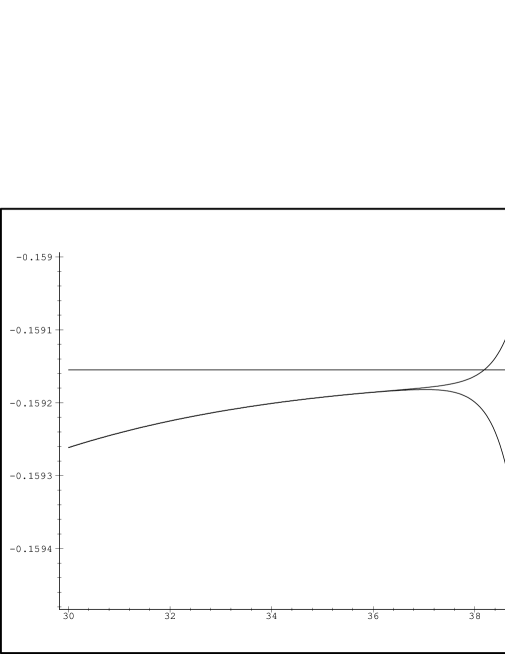
In Figure 1 we have plotted $S_{40}(\lambda,\tau)$ and $S_{39}(\lambda,\tau)$ for three values of $\tau$, namely $\tau=1,2,3$. The last term in $S_{40}(\lambda,\tau)$ is significant where each pair of curves can be seen to diverge. The flatness of the curves for slightly smaller values of $\lambda$ shows that there the value of the truncated series provides a good approximation to the value of the full series as $\lambda\rightarrow\infty$. We have used this to estimate the limit in Figure 2 where we have plotted $S_{40}(\tau,\lambda)$ with $\lambda$ chosen so that the magnitude of the last term in this series is equal to $1/200$, which represents about one per cent of the value of the series for large $\tau$, (varying this fraction by an order of magnitude either way makes little difference). Now from (77) we should have that the limit as $\lambda\rightarrow\infty$ of $S_{\infty}(\lambda,\tau)$ be $(1+e^{2\tau})/(2(1-e^{2\tau}))\equiv f(\tau)$ and this curve is also shown in Figure 2. We can see that $S_{40}$ provides a good approximation for values of $\tau$ up to about 20 which is a long way beyond the region of convergence of the original series $\sum_{0}^{39}b_{n}\tau^{2n-1}\equiv S_{\rm orig}$ from which we have built $S_{40}$ which is also shown in the Figure diverging from the other two curves at $\tau=\pi$.

Figure 2: Tree-level Schrödinger functional: $\Xi_{2}$

In Appendix C we calculate the coefficients $c_{n}$ in the local expansion of $\Xi_{3}$.

$$\Xi_{3}={\tau\over g_{0}^{2}}\sum_{n=0}^{\infty}c_{n}(\tau^{2}V_{2}\cdot)^{n}V_{3}$$ (83)

and the coefficients $f_{n}$ and $h_{p,q,r}$ in the local expansion of $\Xi_{4}$

$$\Xi_{4}={\tau\over g_{0}^{2}}\sum_{n=0}^{\infty}f_{n}(\tau^{2}V_{2}\cdot)^{n}V_{4}+{\tau\over g_{0}^{2}}\sum_{p,q,r}h_{p,q,r}\tau^{2(p+q+r+1)}(V_{2}\cdot)^{p}\left(\left((V_{2}\cdot)^{q}V_{3}\right)\cdot\left((V_{2}\cdot)^{r}V_{3}\right)\right)$$ (84)

In principle we could use this result to compute the one-loop beta-function. The combinatorics are rather daunting compared to the approach we will describe in the next section.

4 Background Field approach, and the beta-function

Recently Zarembo has shown how to calculate the beta-function for Yang-Mills theory using the Schrödinger equation for the vacuum functional with a background field method [12]. As usual the background field approach works especially well at one-loop by reducing the problem to the evaluation of certain coefficents in the asymptotic expansion of a heat-kernel. We will extend this approach to the Schrödinger functional and use it to show that the usual beta-function is obtained from our local expansion. This is important because the beta-function is sensitive only to high momentum modes and so obtaining the correct result shows that we can indeed reconstruct rapidly varying modes from the slowly varying modes of the local expansion using analyticity. The basic idea is to write ${\bf A}$ and $\mbox{${\bf A}$}^{\prime}$ as fluctuations, ${\bf a}$ and $\mbox{${\bf a}$}^{\prime}$, about a background field ${\mbox{${\bf A}$}_{0}}$:

$$\mbox{${\bf A}$}={\mbox{${\bf A}$}_{0}}+\mbox{${\bf a}$},\quad\mbox{${\bf A}$}^{\prime}={\mbox{${\bf A}$}_{0}}+\mbox{${\bf a}$}^{\prime}.$$ (85)

${\bf a}$ is now the dynamical variable so

$${\delta\over\delta A}={\delta\over\delta a}.$$ (86)

The potential term in the Schrödinger equation, $\cal B$ can be expanded up to terms quadratic in ${\bf a}$ as

$${\cal B}={\cal B}_{0}+\mbox{${\bf a}$}\cdot(\mbox{${\bf a}$}\cdot\Lambda)+{\rm Order}(\mbox{${\bf a}$}^{3})$$ (87)

where ${\cal B}_{0}$ is the integral of the square of the magnetic field made from $\mbox{${\bf A}$}_{0}$, i.e. ${\bf B}_{0}=\nabla\wedge\mbox{${\bf A}$}_{0}+\mbox{${\bf A}$}_{0}\wedge\mbox{${\bf A}$}_{0}$, and

$$\Lambda\mbox{${\bf a}$} = -\mbox{${\bf{\cal D}}$}\cdot\mbox{${\bf{\cal D}}$}\mbox{${\bf a}$}+\mbox{${\bf{\cal D}}$}\mbox{${\bf{\cal D}}$}\cdot\mbox{${\bf a}$}+2{\bf B}_{0}\wedge\mbox{${\bf a}$}+2\mbox{${\bf a}$}\wedge{\bf B}_{0}$$ (88)

$$\equiv -\mbox{${\bf{\cal D}}$}\cdot\mbox{${\bf{\cal D}}$}\mbox{${\bf a}$}+\mbox{${\bf{\cal D}}$}\mbox{${\bf{\cal D}}$}\cdot\mbox{${\bf a}$}-2{\bf F}\cdot\mbox{${\bf a}$},$$

where $\cal D$ is given by ${\cal D}\omega=[\nabla+{\bf A}_{0},\omega]$. There is no term linear in ${\bf a}$ since we will take $\mbox{${\bf A}$}_{0}$ to satisfy the three-dimensional Yang-Mills equation $\mbox{${\bf{\cal D}}$}\wedge\mbox{${\bf A}$}_{0}=0$. Consequently when we expand $W[\mbox{${\bf A}$},\mbox{${\bf A}$}^{\prime}]$ in powers of ${\bf a}$ and $\mbox{${\bf a}$}^{\prime}$ there will be no linear terms. If we write the tree-level contribution to $W[\mbox{${\bf A}$},\mbox{${\bf A}$}^{\prime}]$ that is quadratic in the fluctuations as $1/\hbar$ times

$$\mbox{${\bf a}$}\cdot(\mbox{${\bf a}$}\cdot\Xi)+\mbox{${\bf a}$}^{\prime}\cdot(\mbox{${\bf a}$}\cdot\Upsilon)+\mbox{${\bf a}$}^{\prime}\cdot(\mbox{${\bf a}$}^{\prime}\cdot\Xi)$$ (89)

then $\Xi$ and $\Upsilon$ are functionals of the background field $\mbox{${\bf A}$}_{0}$ as well as being functions of $\tau$. Substituting this into the Schrödinger equation (67) and extracting the leading term in $\hbar$ that is quadratic in ${\bf a}$ leads to the same equation as (73) but with $\Xi_{2}$ replaced by $\Xi$ and $V_{2}$ replaced by $\Lambda$. Consequently $\Xi$ has the local expansion

$$\Xi={1\over g_{0}^{2}\tau}\sum_{n=0}^{\infty}b_{n}(\tau^{2}\Lambda\cdot)^{n}$$ (90)

with the same coefficients, $b_{n}$, as before. The expansion is valid for fields that vary slowly on the scale of $\tau$. This tree-level result gives a one-loop contribution to the renormalisation of $g^{2}$ via the condition (63). Since $\cal B$ has the expansion (87) it is sufficent to look at the coefficent of ${\cal B}_{0}$, and this comes from $\Delta_{s}\,(\mbox{${\bf a}$}\cdot(\mbox{${\bf a}$}\cdot\Xi))$. So to order $\hbar$

$${1\over g^{4}(s)}={1\over g_{0}^{4}}+\lim_{\tau\rightarrow\infty}\hbar\Delta_{s}\,\left(\mbox{${\bf a}$}\cdot(\mbox{${\bf a}$}\cdot\Xi)\right)|_{{\cal B}_{0}}$$ (91)

If we introduce the mass-scale $\mu$ by setting $s=\rho/\mu^{2}$, then the beta-function is

$$\beta=\lim_{\rho\downarrow 0}\mu{\partial(g^{2}(\rho/\mu^{2}))\over\partial\mu}=\lim_{\tau\rightarrow\infty,\rho\rightarrow 0}\hbar g^{6}s{\partial\over\partial s}\Delta_{s}\,\left(\mbox{${\bf a}$}\cdot(\mbox{${\bf a}$}\cdot\Xi)\right)|_{{\cal B}_{0}}$$ (92)

Direct substitution of (90) into this would be invalid because as $\rho\rightarrow 0$ the Laplacian includes differentiation with respect to rapidly fluctuating fields which are absent from the local expansion. As we have shown, however, the former can be obtained from the latter by analyticity, and this is encoded into the $R_{\lambda}^{\prime}$ operator. For large $s$

$$\Delta_{s}\,\mbox{${\bf a}$}\cdot(\mbox{${\bf a}$}\cdot\Xi)=2\,TrK\,\left({1\over g^{2}_{0}\tau}\sum_{n=0}^{\infty}b_{n}(\tau^{2}\Lambda\cdot)^{n}\right),$$ (93)

where $Tr$ denotes the functional trace. Previously we chose the kernel, $K$, in the Laplacian to have a simple form in terms of a momentum cut-off multiplied by a Wilson line, but we are free to make other choices provided that we preserve gauge invariance, that the kernel represents a $\delta$-function as the cut-off is removed, and that it scales covariantly. It is particularly convenient for the present calculation to take $K$ to be the heat-kernel of the operator $\Lambda$ at time $s$, thus $K=\exp(-s\Lambda)$ and so the various powers of $\Lambda$ acting on the kernel are obtained by differention with respect to $s$

$$s{\partial\over\partial s}\Delta_{s}\,\mbox{${\bf a}$}\cdot(\mbox{${\bf a}$}\cdot\Xi)=2s{1\over g^{2}_{0}\tau}\sum_{n=0}^{\infty}b_{n}\left(-\tau^{2}{\partial\over\partial s}\right)^{n}{\partial\over\partial s}\,Tr\,\left(K\right).$$ (94)

In Appendix D we use the results of [11] to show that

$$s{\partial\over\partial s}\Delta_{s}\,\mbox{${\bf a}$}\cdot(\mbox{${\bf a}$}\cdot\Xi)\Big{|}_{{\cal B}_{0}}={22N\over 3}{1\over(4\pi)^{3/2}}\sum_{n=0}^{\infty}b_{n}{\Gamma(n+1/2)\over\Gamma(1/2)}\left({\tau^{2}\over s}\right)^{n-1/2}$$ (95)

If we put $s=\rho/\mu^{2}$ the series converges only for large $\rho$, but represents a function that is analytic in the complex $\rho$-plane cut along the negative real axis. If we multiply by $\sqrt{\rho}$ the resulting large-$\rho$ series has only integer powers so the cut for this function has only finite length. Consequently we can obtain the small-$s$ value as

$$\lim_{s\downarrow 0}s{\partial\over\partial s}\Delta_{s}\,\mbox{${\bf a}$}\cdot(\mbox{${\bf a}$}\cdot\Xi)\Big{|}_{{\cal B}_{0}}=$$

$$\lim_{\lambda\rightarrow\infty}{1\over 2\sqrt{\pi}i}\int_{C}{d\rho\over\rho}\,e^{\lambda\rho}\,\sqrt{\lambda\rho}{22N\over 3}{1\over(4\pi)^{3/2}}\sum_{n=0}^{\infty}b_{n}{\Gamma(n+1/2)\over\Gamma(1/2)}\left({\tau^{2}\mu^{2}\over\rho}\right)^{n-1/2}$$ (96)

If the contour $C$ is collapsed to one around the cut consisting of a small circle centred on the origin, $C^{\prime\prime}$, and the rest consisting of two lines slightly above and below the negative real axis, then the contribution of the latter is damped by the $\exp(\lambda\rho)$ factor and the contribution of the former yields the left-hand side because

$$\lim_{\lambda\rightarrow\infty}{1\over 2\pi i}\int_{C^{\prime\prime}}{d\rho\over\rho}\,e^{\lambda\rho}\,\sqrt{\lambda\rho}=\sqrt{\pi}\,.$$ (97)

Performing the contour integration gives

$${22N\over 3}{1\over(4\pi)^{3/2}}\lim_{\lambda\rightarrow\infty}\sum_{n=0}^{\infty}b_{n}{\Gamma(n+1/2)\over\Gamma(n)}\left({\lambda\tau^{2}\mu^{2}}\right)^{n-1/2}$$ (98)

Using the same argument as previously the convergence can be improved by doing a further contour integral in the complex $1/\sqrt{\lambda}$ cut along the negative real axis to obtain

$${22N\over 3}{1\over(4\pi)^{3/2}}\lim_{\lambda\rightarrow\infty}{1\over 2\sqrt{\pi}i}\int_{C^{\prime\prime}}{d\rho\over\rho}\,e^{\lambda^{2}\rho}\,\sqrt{\lambda^{2}\rho}\sum_{n=0}^{\infty}b_{n}{\Gamma(n+1/2)\over\Gamma(n)}\left({\tau^{2}\mu^{2}\over\sqrt{\rho}}\right)^{n-1/2}$$ (99)

which gives the $\beta$-function as

$$\beta=\hbar g^{4}{11N\over 12\pi}\lim_{\lambda,\tau\rightarrow\infty}\sum_{n=0}^{\infty}b_{n}{\Gamma(n+1/2)\over\Gamma(n)\,\Gamma(n/2+1/4)}\left({\lambda\tau^{2}\mu^{2}}\right)^{n-1/2}.$$ (100)

Figure 3: The series $S_{99}^{\beta}$ and $S_{100}^{\beta}$

In Figure 3 we have shown as a function of $x$ the finite sum

$$S^{\beta}_{N}(x)\equiv\sum_{n=0}^{N}b_{n}{\Gamma(n+1/2)\over\Gamma(n)\,\Gamma(n/2+1/4)}x^{n-1/2}.$$ (101)

for $N=100$ and $N=99$. These sums are seen to diverge for $x\approx 39$ which is when the last term of the former series begins to have a non-negligible value. We can trust the finite sum $S_{100}^{\beta}$ as a good approximation to $S_{\infty}^{\beta}(x)$ up to this value of $x$. From the known value of the $\beta$-function the limit of this series should be

$$\lim_{x\rightarrow\infty}S_{\infty}^{\beta}(x)=-{1\over 2\pi}$$ (102)

and this value is shown as the stright line in the figure. From this it is clear that the limit is well approximated by taking the value of the finite sums just before they diverge. In Figure 4 we have shown the same curves over a shorter range of $x$, from which we can see that this procedure for estimating the limit gives the numerical value $S^{\beta}_{100}(37)=-0.15918$ which as an estimate of $-1/(2\pi)\approx-0.159155$ is correct to about two parts in $10^{4}$.

Figure 4: The series $S_{99}^{\beta}$ and $S_{100}^{\beta}$

The error may be estimated a priori by examining how the curve $S^{\beta}_{100}$ approaches the straight line that represents its limiting value. From the method we employed to suppress the contribution of the cut we would expect that the deviation from a stright-line is roughly exponential in $\lambda$ for large $\lambda$. In Figure 5 we have shown the logarithm of the derivative of $S^{\beta}_{100}(x)$ which shows that this is indeed approximately linear in $x$ with slope $\approx-1/5$, hence $S^{\beta}_{100}\approx A+B\exp(-x/5)$. The error in approximating $\lim{\lambda\rightarrow\infty}\quad S_{\infty}^{\beta}$ by $S^{\beta}_{100}(37)$ is thus of the order of $B\exp(-x/5)\approx|5\,S^{\beta^{\prime}}_{100}(37)|\approx 2.4\times 10^{-4}$.

Figure 5: $\log(S_{100}^{\beta^{\prime}}(x))$

5 Conclusions

When a scaling ${\bf x}\rightarrow{\bf x}/\sqrt{\rho}$ is applied to a quantum field theory many quantities can be continued to analytic functions in the complex $\rho$-plane cut along the negative real axis. We have seen this to be the case for the connected Green’s functions that contribute to the logarithm of the Schrödinger functional, and also for appropriately defined bare couplings, (and consequently their beta-functions). It is also a property of, for example, the two-point function of Lorentz invariant operators as can be seen from the Källen-Lehmann representation, and of the Zamolodchikov c-function. We have exploited this analyticity to reconstruct the Schrödinger functional for arbitrarily varying fields from its expression as a local expansion that is valid for slowly varying fields, and we have obtained the form of the Schrödinger equation that acts directly on this local expansion. This leads to coupled algebraic equations that may, in principle, be solved without recourse to perturbation theory, but our purpose here has been to show that when these equations are solved in powers of the coupling they are in agreement with the expected results of perturbation theory. To make this comparison we first solved the functional Schrödinger equation in a ‘standard’ perturbative manner without using the local expansion. We also computed the beta-function in both approaches and obtained the usual result. This illustrates that short-distance effects can be correctly reproduced from our small momentum expansion because the beta-function is a consequence of rapidly varying field configurations.

Appendix A Tree-level contribution to $W[\mbox{${\bf A}$}]$

In this appendix we calculate the tree-level contributions to $W[\mbox{${\bf A}$}]$ up to fourth order, i.e. $W_{0}^{2}$, $W_{2}^{3}$ and $W_{0}^{4}$.

A.1 Calculating $W_{0}^{2}$

The Hamilton-Jacobi equation gives

$$g_{0}^{4}\int{d^{3}p\over(2\pi)^{3}}\frac{\mbox{$\delta$}W_{0}^{2}}{\mbox{$\delta$}A^{R}_{\alpha}({\bf p})}\frac{\mbox{$\delta$}W_{0}^{2}}{\mbox{$\delta$}A^{R}_{\alpha}(-{\bf p})}={\cal B}_{2}\,,$$ (103)

in which ${\cal B}_{2}$ is the part of the potential ${\cal B}$ that is quadratic in $A$:

$${\cal B}_{2} = \int{d^{3}p\over(2\pi)^{3}}({\bf p}\wedge\mbox{${\bf A}$}^{A}({\bf p}))\cdot({\bf p}\wedge\mbox{${\bf A}$}^{A}(-{\bf p}))$$ (104)

$$= \int{d^{3}p\over(2\pi)^{3}}A_{\alpha}^{A}({\bf p})A_{\beta}^{A}(-{\bf p})\,\,({\bf p}^{2}\mbox{$\delta$}^{\alpha\beta}-p^{\alpha}p^{\beta})\,\,,$$

We can take $W_{0}^{2}$ to have the form

$$W_{0}^{2}={1\over g_{0}^{2}}\int{d^{3}p\over(2\pi)^{3}}A_{\mu}^{A}({\bf p})A_{\nu}^{A}(-{\bf p})\,\,\Gamma^{\mu\nu}({\bf p}),\quad\Gamma^{\nu\mu}(-{\bf p})=\Gamma^{\mu\nu}({\bf p})$$ (105)

Hence

$$\frac{\mbox{$\delta$}W_{0}^{2}}{\mbox{$\delta$}A^{R}_{\alpha}({\bf p})}={2\over g_{0}^{2}}\Gamma^{\alpha\nu}({\bf p})A_{\nu}^{R}(-{\bf p})$$ (106)

so that the Hamilton-Jacobi equation and Gauss’ law become

$$4\Gamma^{\mu\alpha}({\bf p})\delta_{\alpha\beta}\Gamma^{\beta\nu}({\bf p})={\bf p}^{2}\mbox{$\delta$}^{\mu\nu}-p^{\mu}p^{\nu}\,,\quad p_{\mu}\Gamma^{\mu\nu}({\bf p})=0$$ (107)

which has the solution

$$\Gamma_{\alpha\beta}({\bf p})=\frac{p_{\alpha}p_{\beta}-{\bf p}^{2}\mbox{$\delta$}_{\alpha\beta}}{2|{\bf p}|}.$$ (108)

This is unique up to a sign which is chosen to make $\Psi$ square integrable to this order.

A.2 Calculating $W_{0}^{3}$

To third order in ${\bf A}$ the Hamilton-Jacobi equation is

$$2g_{0}^{4}\int{d^{3}p\over(2\pi)^{3}}\frac{\mbox{$\delta$}W_{0}^{2}}{\mbox{$\delta$}A^{R}_{\eta}(-{\bf p})}\frac{\mbox{$\delta$}W_{0}^{3}}{\mbox{$\delta$}A^{R}_{\eta}({\bf p})}={\cal B}_{3}$$ (109)

with

$${\cal B}_{3}=-i\,\int{d^{3}p_{1}\,d^{3}p_{2}\,d^{3}p_{3}\over(2\pi)^{6}}\mbox{$\delta$}^{3}({\bf p}_{1}+{\bf p}_{2}+{\bf p}_{3})({\bf p}_{1}\wedge\mbox{${\bf A}$}^{A}({\bf p}_{1}))\cdot(\mbox{${\bf A}$}^{B}({\bf p}_{2})\wedge\mbox{${\bf A}$}^{C}({\bf p}_{3}))\,\,f^{ABC}\,.$$ (110)

$W_{0}^{3}$ has the form

$$W_{0}^{3}={1\over g_{0}^{2}}\int{d^{3}p_{1}\,d^{3}p_{2}\,d^{3}p_{3}\over(2\pi)^{6}}A_{\alpha}^{A}({\bf p}_{1})A_{\beta}^{B}({\bf p}_{2})A_{\gamma}^{C}({\bf p}_{3})\,\,\,f^{ABC}\,\Gamma^{\alpha\beta\gamma}({\bf p}_{1},{\bf p}_{2},{\bf p}_{3})\,\mbox{$\delta$}^{3}({\bf p}_{1}+{\bf p}_{2}+{\bf p}_{3})\,\,.$$ (111)

The sign of $\Gamma^{\alpha\beta\gamma}({\bf p}_{1},{\bf p}_{2},{\bf p}_{3})$ changes if we simultaneously interchange any two momenta and their respective indices, as it does if we reverse all the momenta. (109) becomes

$$\int{d^{3}p_{1}\,d^{3}p_{2}\,d^{3}p_{3}}\,A_{\alpha}^{A}({\bf p}_{1})A_{\beta}^{B}({\bf p}_{2})A_{\gamma}^{C}({\bf p}_{3})\,\,\,\,\mbox{$\delta$}^{3}({\bf p}_{1}+{\bf p}_{2}+{\bf p}_{3})$$

$${\Big{\{}}f^{ABC}\left(12\Gamma_{\eta}^{\alpha}({\bf p}_{1})\Gamma^{\eta\beta\gamma}({\bf p}_{1},{\bf p}_{2},{\bf p}_{3})+ip_{1\eta}\delta^{\eta\alpha}_{\beta\gamma}\right){\Big{\}}}=0\,,$$ (112)

implying

$${\cal S}{\Big{\{}}f^{ABC}\left(12\,\Gamma_{\eta\alpha}({\bf p}_{1})\Gamma_{\eta\beta\gamma}({\bf p}_{1},{\bf p}_{2},{\bf p}_{3})+ip_{1\eta}\delta^{\eta\alpha}_{\beta\gamma}\right){\Big{\}}}=0\,.$$ (113)

${\cal S}$ standing for symmetrisation under interchange of the sets $\{A,\alpha,{\bf p}_{1}\}$, $\{B,\beta,{\bf p}_{2}\}$, and $\{C,\gamma,{\bf p}_{3}\}$, giving

$$4f^{ABC}{\Big{\{}}\Gamma_{\alpha\eta}({\bf p}_{1})\Gamma_{\eta\beta\gamma}({\bf p}_{1},{\bf p}_{2},{\bf p}_{3})+\Gamma_{\beta\eta}({\bf p}_{2})\Gamma_{\alpha\eta\gamma}({\bf p}_{1},{\bf p}_{2},{\bf p}_{3})+\Gamma_{\gamma\eta}({\bf p}_{3})\Gamma_{\alpha\beta\eta}({\bf p}_{1},{\bf p}_{2},{\bf p}_{3}){\Big{\}}}$$ (114)

for the first term between braces and

$$\frac{1}{3}f^{ABC}{\Big{\{}}p_{1\eta}\delta^{\eta\alpha}_{\beta\gamma}+p_{2\eta}\delta^{\eta\beta}_{\gamma\alpha}+p_{3\eta}\delta^{\eta\gamma}_{\alpha\beta}{\Big{\}}}$$ (115)

for the second. Gauss’s law (8) for $W_{0}^{3}$ states that

$$-i{\bf p}.\frac{\mbox{$\delta$}W_{0}^{3}}{\mbox{$\delta$}\mbox{${\bf A}$}^{R}(-{\bf p})}=-f^{RST}\int{d^{3}q\over(2\pi)^{3}}\mbox{${\bf A}$}^{S}({\bf p}-{\bf q})\frac{\mbox{$\delta$}W_{0}^{2}}{\mbox{$\delta$}\mbox{${\bf A}$}^{T}(-{\bf q})}$$ (116)

which can be written as

$$p_{1\alpha}\Gamma_{\alpha\beta\gamma}({\bf p}_{1},{\bf p}_{2},-{\bf p}_{1}-{\bf p}_{2})=\frac{i}{3}\Big{(}\Gamma_{\beta\gamma}({\bf p}_{3})-\Gamma_{\beta\gamma}({\bf p}_{2})\Big{)}\,\,\,$$ (117)

(117) and (113) have the solution

$$\Gamma_{\alpha\beta\gamma}({\bf p}_{1},{\bf p}_{2},{\bf p}_{3})=$$ (118)

$$\frac{i}{3(|{\bf p}_{1}|+|{\bf p}_{2}|+|{\bf p}_{3}|)}\times{\Bigg{\{}}+\hat{p}_{1\alpha}(\Gamma_{\beta\gamma}({\bf p}_{3})-\Gamma_{\beta\gamma}({\bf p}_{2}))-\hat{p}_{2\beta}(\Gamma_{\alpha\gamma}({\bf p}_{3})$$

$$- \Gamma_{\alpha\gamma}({\bf p}_{1}))-\hat{p}_{3\gamma}(\Gamma_{\alpha\beta}({\bf p}_{1})-\Gamma_{\alpha\beta}({\bf p}_{2}))+\frac{1}{2}(p_{1\eta}\delta^{\eta\alpha}_{\beta\gamma}+p_{2\eta}\delta^{\eta\beta}_{\gamma\alpha}+p_{3\eta}\delta^{\eta\gamma}_{\alpha\beta}){\Bigg{\}}}$$

A.3 Calculating $W_{0}^{4}$

The quartic terms in the Hamilton-Jacobi equation yield:

$$g_{0}^{4}\int{d^{3}p\over(2\pi)^{3}}\Bigg{(}2\frac{\mbox{$\delta$}W_{0}^{2}}{\mbox{$\delta$}A^{R}_{\alpha}(-{\bf p})}\frac{\mbox{$\delta$}W_{0}^{4}}{\mbox{$\delta$}A^{R}_{\alpha}({\bf p})}+\frac{\mbox{$\delta$}W_{0}^{3}}{\mbox{$\delta$}A^{R}_{\alpha}(-{\bf p})}\frac{\mbox{$\delta$}W_{0}^{3}}{\mbox{$\delta$}A^{R}_{\alpha}({\bf p})}\Bigg{)}={\cal{B}}_{4}.$$ (119)

We take $W_{0}^{4}$ to have the form

$$W_{0}^{4} = {1\over g_{0}^{2}}\int{d^{3}p_{1}\,d^{3}p_{2}\,d^{3}p_{3}\,d^{3}p_{4}\over(2\pi)^{9}}\mbox{$\delta$}^{3}({\bf p}_{1}+{\bf p}_{2}+{\bf p}_{3}+{\bf p}_{4})\,A_{\alpha}^{A}({\bf p}_{1})A_{\beta}^{C}({\bf p}_{2})A_{\gamma}^{B}({\bf p}_{3})A_{\delta}^{D}({\bf p}_{4})\times$$ (120)

$$\times f^{MAB}f^{MCD}\Gamma_{\alpha\beta\gamma\delta}({\bf p}_{1},{\bf p}_{2},{\bf p}_{3},{\bf p}_{4})\,.$$

The quartic term of the potential is

$${\cal{B}}_{4} = {1\over 4}\int{d^{3}p_{1}\,d^{3}p_{2}\,d^{3}p_{3}\,d^{3}p_{4}\over(2\pi)^{9}}\mbox{$\delta$}^{3}({\bf p}_{1}+{\bf p}_{2}+{\bf p}_{3}+{\bf p}_{4})\,A_{\alpha}^{A}({\bf p}_{1})A_{\beta}^{C}({\bf p}_{2})A_{\gamma}^{B}({\bf p}_{3})A_{\delta}^{D}({\bf p}_{4})\times$$ (121)

$$\times f^{MAB}f^{MCD}\mbox{$\delta$}^{\alpha\beta}_{\gamma\delta}\,.$$

The Hamilton-Jacobi equation implies that

$${\cal{S}}_{4}{\Big{\{}}f^{MAB}f^{MCD}\Big{(}16\Gamma_{\alpha\eta}({\bf p}_{1})\Gamma_{\eta\beta\gamma\delta}({\bf p}_{1},{\bf p}_{2},{\bf p}_{3},{\bf p}_{4})+$$

$$9\,\Gamma_{\eta\alpha\beta}({\bf p}_{3}+{\bf p}_{4},{\bf p}_{1},{\bf p}_{2})\Gamma_{\eta\gamma\delta}({\bf p}_{1}+{\bf p}_{2},{\bf p}_{3},{\bf p}_{4})-{1\over 4}\mbox{$\delta$}^{\alpha\beta}_{\gamma\delta}\Big{)}{\Big{\}}}=0\,,$$ (122)

Where ${\cal S}_{4}$ symmetrises the expression under simultaneous interchanges of the four sets of indices and momenta $A,\alpha,{\bf p}_{1}$ etc. Gauss’s law for $W_{0}^{4}$,

$$i{\bf p}.\frac{\mbox{$\delta$}W_{0}^{4}}{\mbox{$\delta$}\mbox{${\bf A}$}^{R}({\bf p})}=-f^{RST}\int{d^{3}q\over(2\pi)^{3}}\mbox{${\bf A}$}^{S}(-{\bf p}-{\bf q})\frac{\mbox{$\delta$}W_{0}^{3}}{\mbox{$\delta$}\mbox{${\bf A}$}^{T}(-{\bf q})}\,,$$ (123)

can be expressed as

$${\cal S}_{3}\left\{f^{MNA}f^{MCD}\left(4p_{\eta}\Gamma_{\eta\alpha\beta\gamma}({\bf p},{\bf p}_{1},{\bf p}_{2},{\bf p}_{3})-3i\,\,\Gamma_{\alpha\beta\gamma}({\bf p}+{\bf p}_{1},{\bf p}_{2},{\bf p}_{3})\right)\right\}$$

$${\mbox{when}}\,\,\,\,\,\,{\bf p}+{\bf p}_{1}+{\bf p}_{2}+{\bf p}_{3}=0\,,$$ (124)

and ${\cal S}_{3}$ denotes symmetrisation under interchange of the three sets $\{A,\alpha,{\bf p}_{1}\}$, $\{B,\beta,{\bf p}_{2}\}$ and $\{C,\gamma,{\bf p}_{3}\}$. Using this in (122) we find

$${\cal{S}}_{4}{\Big{\{}}f^{MAB}f^{MCD}\Gamma_{\alpha\beta\gamma\delta}({\bf p}_{1},{\bf p}_{2},{\bf p}_{3},{\bf p}_{4})\Big{\}}=$$

$${\cal{S}}_{4}{\Big{\{}}f^{MAB}f^{MCD}\omega\Big{(}6i{\hat{p}}_{1\alpha}\Gamma_{\beta\gamma\delta}({\bf p}_{1}+{\bf p}_{2},{\bf p}_{3},{\bf p}_{4})+$$

$$\,\,\,\,\,\,\,\,\,\,\,\ +9\,\Gamma_{\eta\alpha\beta}({\bf p}_{3}+{\bf p}_{4},{\bf p}_{1},{\bf p}_{2})\Gamma_{\eta\gamma\delta}({\bf p}_{1}+{\bf p}_{2},{\bf p}_{3},{\bf p}_{4})-{1\over 4}\mbox{$\delta$}^{\alpha\beta}_{\gamma\delta}\Big{)}{\Big{\}}}$$ (125)

where

$$\omega={1\over 2(|{\bf p}_{1}|+|{\bf p}_{2}|+|{\bf p}_{3}|+|{\bf p}_{4}|)}$$ (126)

Appendix B Contributions to the one loop Beta-function

In this appendix we calculate the small $s$ behaviour of $\Delta_{s}W_{0}^{2}$, $\Delta_{s}W_{0}^{3}$ and $\Delta_{s}W_{0}^{4}$.

B.1 $\Delta_{s}W_{0}^{2}$

Since $W_{0}^{2}$ is only quadratic in ${\bf A}$ the ${\bf A}$-dependence of $\Delta_{s}W_{0}^{2}$ derives from the Wilson line in the reulator kernel. The term that is quadratic in $A$ is thus

$$\Big{(}\Delta_{s}g_{0}^{2}\,W_{0}^{2}\Big{)}_{A^{2}}=\int_{|{\bf p}|^{2}<1/s}{d^{3}x\,d^{3}y\,d^{3}q\,d^{3}p\over(2\pi)^{6}}e^{i\,{\bf p}({\bf x}-{\bf y})}\Big{[}U^{RS}({\bf x},{\bf y})\Big{]}_{A^{2}}\,2\,e^{-i\,{\bf{q}}({\bf x}-{\bf y})}\mbox{$\delta$}^{RS}\Gamma_{\rho\rho}(q)\,,$$ (127)

where

$$\Big{[}U^{RS}({\bf x},{\bf y})\Big{]}_{A^{2}}={\cal{P}}\,\Bigg{(}\frac{1}{2}\int_{{\bf x}}^{{\bf y}}d{\mbox{w}}_{\mu}\int_{{\bf x}}^{{\bf y}}d{\mbox{z}}_{\nu}\,A^{A}_{\mu}({\bf{w}})A^{B}_{\nu}({\bf{z}})\,T^{A}T^{B}\Bigg{)}_{RS}\,.$$ (128)

We parametrise the integration path as

$${\bf{w}} = {\bf x}+\sigma_{1}({\bf y}-{\bf x})\,,\quad 0\leq\sigma_{1}\leq 1$$

$${\bf{z}} = {\bf x}+\sigma_{2}({\bf y}-{\bf x})\,,\quad 0\leq\sigma_{2}\leq 1\,,$$ (129)

and change the variables such that ${\bf y}\rightarrow{\bf{v}}=({\bf y}-{\bf x})$. Then, after integrating over ${\bf x}$, we get

$$\Big{(}\Delta_{s}g_{0}^{2}\,W_{0}^{2}\Big{)}_{A^{2}}=$$

$$-\,\int d^{3}v\,d^{3}q\,d^{3}k\,d^{3}k^{\prime}\,d^{3}p\,d\sigma_{1}\,d\sigma_{2}\,(2\pi)^{-9}\mbox{$\delta$}^{3}({\bf{k}}+{\bf{k}}^{\prime})\,A_{\mu}^{A}({\bf{k}})A_{\nu}^{B}({\bf{k}}^{\prime})$$

$$\times e^{i\,{\bf{v}}.({\bf q}+\sigma_{1}{\bf{k}}+\sigma_{2}{\bf{k}}^{\prime}-{\bf p})}|{\bf q}|\,{\mbox{v}}_{\mu}{\mbox{v}}_{\nu}(T^{A}T^{B})_{RR}\,,$$ (130)

where the integration is restricted by $|{\bf p}|^{2}<1/s,0\leq\sigma_{1}\leq 1,0\leq\sigma_{2}\leq 1$. Finally, integrating (130) over ${\bf{k}}^{\prime}$ and ${\bf{v}}$ allows us to write

$$\Big{(}\Delta_{s}g_{0}^{2}\,W_{0}^{2}\Big{)}_{A^{2}}=-{N\over(2\pi)^{6}}\,\int\int d^{3}q\,d^{3}k\,d^{3}p\,d\sigma_{1}\,d\sigma_{2}\,A_{\mu}^{A}({\bf{k}})A_{\nu}^{A}(-{\bf{k}})$$

$$\frac{\partial^{2}}{\partial q_{\mu}\partial q_{\nu}}\Bigg{[}\mbox{$\delta$}^{3}({\bf q}+{\bf{k}}(\sigma_{1}-\sigma_{2})-{\bf p})\Bigg{]}\,\,|{\bf q}|\,,$$ (131)

We can integrate by parts to make the two derivatives act on $|{\bf q}|$, and use

$$\frac{\partial^{2}|{\bf q}|}{\partial q_{\mu}\partial q_{\nu}}=\frac{1}{|{\bf q}|}\Bigg{(}\mbox{$\delta$}_{\mu\nu}-\frac{q_{\mu}q_{\nu}}{|{\bf q}|^{2}}\Bigg{)}.$$ (132)

This gives

$$-{N\over(2\pi)^{6}}\,\int d^{3}q\,d^{3}k\,d^{3}p\,d\sigma_{1}\,d\sigma_{2}\,A_{\mu}^{A}({\bf{k}})A_{\nu}^{A}(-{\bf{k}})\,\,\mbox{$\delta$}^{3}({\bf q}+{\bf{k}}(\sigma_{1}-\sigma_{2})-{\bf p})\,\,\frac{1}{|{\bf q}|}\Bigg{(}\mbox{$\delta$}_{\mu\nu}-\frac{q_{\mu}q_{\nu}}{|{\bf q}|^{2}}\Bigg{)}.$$ (133)

If we perform the integration over ${\bf q}$ using the delta function, call $\sigma_{1}-\sigma_{2}=y$ and make a change of variables such that

$$\int_{0}^{1}d\sigma_{2}\int_{0}^{1}d\sigma_{1}=\int_{0}^{1}d\sigma_{2}\int_{-\sigma_{2}}^{1-\sigma_{2}}dy$$ (134)

we end up with

$$-N\,\int{d^{3}k\,d^{3}p\,d\sigma_{2}\,dy\over(2\pi)^{6}}A_{\mu}^{A}({\bf{k}})A_{\nu}^{A}(-{\bf{k}}) \times \,\,\Bigg{\{}\frac{\mbox{$\delta$}_{\mu\nu}}{|{\bf p}-{\bf{k}}y|}-\frac{p_{\mu}p_{\nu}}{|{\bf p}-{\bf{k}}y|^{3}}+\frac{p_{\mu}k_{\nu}y}{|{\bf p}-{\bf{k}}y|^{3}}$$

$$+ \frac{p_{\nu}k_{\mu}y}{|{\bf p}-{\bf{k}}y|^{3}}-\frac{k_{\mu}k_{\nu}y^{2}}{|{\bf p}-{\bf{k}}y|^{3}}\Bigg{\}}$$

$$\equiv\int d^{3}k\,A_{\mu}^{A}({\bf{k}})A_{\nu}^{A}(-{\bf{k}})\Lambda^{\mu\nu}_{2}({\bf{k}})$$ (135)

where $-\sigma_{2}\leq y\leq 1-\sigma_{2}$, $0\leq\sigma_{2}\leq 1$ and $|{\bf p}|^{2}<1/s$.

B.2 $\Delta_{s}W_{0}^{3}$

In this case, the quadratic term is obtained by taking the term that is linear in $A$ in the expansion of $U^{RS}({\bf x},{\bf y})$. Following similar steps as we presented in section (B.1) and using that

$$\frac{\mbox{$\delta$}^{2}W_{0}^{3}}{\mbox{$\delta$}A_{\rho}^{R}({\bf y})\mbox{$\delta$}A_{\rho}^{S}({\bf x})}={6\over g^{2}_{0}}\,\int_{{\bf{z}}}A_{\nu}^{C}({\bf{z}})f^{SRC}\,\Gamma_{\rho\rho\nu}({\bf x},{\bf y},{\bf{z}})\,,$$ (136)

we obtain

$$\Big{(}\Delta_{s}g_{0}^{2}\,W_{0}^{3}\Big{)}_{A^{2}}=-{6i\,N\over(2\pi)^{6}} \int_{\Sigma^{\prime\prime}}d^{3}k\,d^{3}q\,d^{3}p\,A_{\mu}^{A}(-{\bf{k}})A_{\nu}^{A}({\bf{k}})\,\,\mbox{$\delta$}^{3}\Big{(}{\bf p}-{\bf q}+(\sigma-1){\bf{k}}\Big{)}\,\times$$ (137)

$$\times\frac{\partial\Gamma_{\rho\rho\nu}({\bf q},-{\bf q}-{\bf{k}},{\bf{k}})}{\partial q_{\mu}}$$

$$\equiv\int d^{3}k\,A_{\mu}^{A}({\bf{k}})A_{\nu}^{A}(-{\bf{k}})\Lambda^{\mu\nu}_{3}({\bf{k}})$$

where $|{\bf p}|^{2}<1/s$ and $0\leq\sigma\leq 1$.

B.3 $\Delta_{s}W_{0}^{4}$

The term that is quadratic in $A$ receives no contribution from the Wilson line and so is just

$$\Big{(}\Delta_{s}W_{0}^{4}\Big{)}_{A^{2}}=\int_{|{\bf p}|^{2}<1/s}{d^{3}p\over(2\pi)^{3}}e^{i{\bf p}\,({\bf x}-{\bf y})}\mbox{$\delta$}^{RS}\frac{\mbox{$\delta$}^{2}W_{0}^{4}}{\mbox{$\delta$}A^{R}_{\rho}({\bf y})\mbox{$\delta$}A^{S}_{\rho}({\bf x})}\,.$$ (138)

We obtain from (24)

$$\Big{(}\Delta_{s}g_{0}^{2}W_{0}^{4}\Big{)}_{A^{2}}=-N\int_{{\bf{k}},|{\bf p}|^{2}<1/s}A_{\mu}^{A}({\bf{k}})A_{\nu}^{A}(-{\bf{k}})\,\,\,\frac{1}{(|{\bf p}|+|{\bf{k}}|)}{\Bigg{\{}}$$

$$\quad\quad 18\,\Gamma_{\eta\rho\mu}({\bf p}+{\bf{k}},-{\bf p},-{\bf{k}})\Gamma_{\eta\rho\nu}({\bf p}+{\bf{k}},-{\bf p},-{\bf{k}})+6i{\hat{k}}_{\mu}\Gamma_{\nu\rho\rho}(-{\bf{k}},{\bf p}+{\bf{k}},-{\bf p})$$

$$\quad\quad-6i{\hat{p}}_{\rho}\Gamma_{\mu\rho\nu}({\bf p}+{\bf{k}},-{\bf p},-{\bf{k}})+2\,\mbox{$\delta$}^{\mu\nu}{\Bigg{\}}}$$

$$\equiv\int d^{3}k\,A_{\mu}^{A}({\bf{k}})A_{\nu}^{A}(-{\bf{k}})\Lambda^{\mu\nu}_{4}({\bf{k}})$$ (139)

Appendix C Cubic and Quartic Terms in the Schrödinger Functional.

The term in the Schrödinger equation that is cubic in ${\bf A}$ is

$$\lim_{\lambda\rightarrow\infty}R^{\prime}_{\lambda}\,\Big{(}{1\over g^{2}}\mbox{${\bf A}$}^{\rho}\cdot(\mbox{${\bf A}$}^{\rho}\cdot(\mbox{${\bf A}$}^{\rho}\cdot\dot{\Xi}_{3}))-6\mbox{${\bf A}$}^{\rho}\cdot((\mbox{${\bf A}$}^{\rho}\cdot\Xi_{3}))\cdot(\mbox{${\bf A}$}^{\rho}\cdot\Xi_{2})$$

$$\quad\quad+{1\over 2g^{4}}\mbox{${\bf A}$}^{\rho}\cdot(\mbox{${\bf A}$}^{\rho}\cdot(\mbox{${\bf A}$}^{\rho}\cdot V_{3}))\Big{)}=0$$ (140)

We assume an expansion of $\Xi_{3}$ of the form

$$\Xi_{3}={\tau\over g_{0}^{2}}\sum_{n=0}^{\infty}c_{n}(\tau^{2}V_{2}\cdot)^{n}V_{3}$$ (141)

which is again an expansion in powers of derivatives. Using this in 140 leads to

$$\lim_{\lambda\rightarrow\infty}R^{\prime}_{\lambda}\,\rho\Big{(}{1\over\tau^{2}}\sum_{n=0}^{\infty}c_{n}(2n+1)({\tau^{2}\over\rho}V_{2}\cdot)^{n}V_{3}$$

$$\quad\quad-{6}\sum_{n,m=0}^{\infty}b_{n}\,c_{m}\,({\tau^{2}\over\rho}V_{2}\cdot)^{n+m}V_{3}+{1\over 2\rho}V_{3}\Big{)}=0$$ (142)

By equating to zero the coefficients of the various powers of $V_{2}\cdot$ we obtain the $c_{n}$ as

$$c_{0}=-{1\over 8},\quad c_{n}={3\over n+2}\sum_{p=1}^{n-1}b_{n-p}\,c_{p},\quad n>0$$ (143)

Similarly $\Xi_{4}$ can be obtained from the term in the Schrödinger equation that is quartic in $\mbox{${\bf A}$}^{\rho}$

$$\lim_{\lambda\rightarrow\infty}R^{\prime}_{\lambda}\,\Big{(}{1\over g_{0}^{2}}\mbox{${\bf A}$}^{\rho}\cdot(\mbox{${\bf A}$}^{\rho}\cdot(\mbox{${\bf A}$}^{\rho}\cdot(\mbox{${\bf A}$}^{\rho}\cdot\dot{\Xi}_{4})))$$

$$\quad\quad-8\mbox{${\bf A}$}^{\rho}\cdot(\mbox{${\bf A}$}^{\rho}\cdot((\mbox{${\bf A}$}^{\rho}\cdot\Xi_{4})))\cdot(\mbox{${\bf A}$}^{\rho}\cdot\Xi_{2})-{9\over 2}\mbox{${\bf A}$}^{\rho}\cdot((\mbox{${\bf A}$}^{\rho}\cdot\Xi_{3}))\cdot\mbox{${\bf A}$}^{\rho}\cdot((\mbox{${\bf A}$}^{\rho}\cdot\Xi_{3}))$$

$$\quad\quad+{1\over 2g_{0}^{4}}\mbox{${\bf A}$}^{\rho}\cdot(\mbox{${\bf A}$}^{\rho}\cdot(\mbox{${\bf A}$}^{\rho}\cdot(\mbox{${\bf A}$}^{\rho}\cdot V_{4})))\Big{)}=0$$ (144)

Taking $\Xi_{4}$ to have the form

$$\Xi_{4}={\tau\over g_{0}^{2}}\sum_{n=0}^{\infty}f_{n}(\tau^{2}V_{2}\cdot)^{n}V_{4}+{\tau\over g_{0}^{2}}\sum_{p,q,r}h_{p,q,r}\tau^{2(p+q+r+1)}(V_{2}\cdot)^{p}\left(\left((V_{2}\cdot)^{q}V_{3}\right)\cdot\left((V_{2}\cdot)^{r}V_{3}\right)\right)$$ (145)

leads eventually to the following formulae for the coefficents:

$$f_{0}=-{1\over 10},\quad f_{n}={8\over 2n+5}\sum_{p=1}^{n-1}b_{n-p}\,f_{p},\quad n>0$$ (146)

and

$$h_{0,q,r}={9\over 4(q+r)+14}c_{q}c_{r},\quad h_{n,q,r}={8\over 2(n+q+r)+7}\sum_{p=0}^{n-1}b_{n-p}\,h_{p,q,r},\quad n>0$$ (147)

Appendix D Heat-Kernel Results

In [11] it was shown that

$${\partial\over\partial s}\,Tr\,{K}={\partial\over\partial s}\left(Tr\,exp\,\left({s(\mbox{${\bf{\cal D}}$}\cdot\mbox{${\bf{\cal D}}$}{\bf 1}+2{\bf F})\cdot}\right)-Tr\,exp\,\left({s\mbox{${\bf{\cal D}}$}\cdot\mbox{${\bf{\cal D}}$}}\right)\right).$$ (148)

where for background fields that are slowly varying on the scale of $s$

$$exp\,\left({s(\mbox{${\bf{\cal D}}$}\cdot\mbox{${\bf{\cal D}}$}{\bf 1}+2{\bf F})\cdot}\right)^{CD}\delta({\bf x}-{\bf y})\,{\bf 1}={e^{-({\bf x}-{\bf y})^{2}/(4s)}\over{\sqrt{4\pi s}}^{3}}\sum_{n=0}^{\infty}s^{n}{\bf b}_{n}^{BC}({\bf x},{\bf y})$$ (149)

and

$$exp\,\left({s\mbox{${\bf{\cal D}}$}\cdot\mbox{${\bf{\cal D}}$}}\right)^{CD}\delta({\bf x}-{\bf y})={e^{-({\bf x}-{\bf y})^{2}/(4s)}\over{\sqrt{4\pi s}}^{3}}\sum_{n=0}^{\infty}s^{n}{a}_{n}^{BC}({\bf x},{\bf y})$$ (150)

The first few coefficents are, at coincident argument,

$$a_{1}({\bf x},{\bf x})=0,\quad a_{2}({\bf x},{\bf x})={1\over 12}F_{ij}F_{ij}$$ (151)

and

$${\bf b}_{1}({\bf x},{\bf x})=2{\bf F},\quad{\bf b}_{2}({\bf x},{\bf x})=2{\bf F}\cdot{\bf F}+{1\over 12}{\bf 1}\,F_{ij}F_{ij}+{1\over 3}\mbox{${\bf{\cal D}}$}\cdot\mbox{${\bf{\cal D}}$}{\bf F}$$ (152)

Resulting in

$${\partial\over\partial s}\,Tr\,{K}={11N\over 3}{1\over(4\pi)^{3/2}}{1\over\sqrt{s}}{\cal B}_{0}+O(\sqrt{s}).$$ (153)

which gives

$$s{\partial\over\partial s}\Delta_{s}\,\mbox{${\bf a}$}\cdot(\mbox{${\bf a}$}\cdot\Xi)\Big{|}_{{\cal B}_{0}} = {22N\over 3}{1\over(4\pi)^{3/2}}\sum_{n=0}^{\infty}b_{n}\,{s\over\tau}\left(-\tau^{2}{\partial\over\partial s}\right)^{n}{1\over\sqrt{s}}$$ (154)

$$= {22N\over 3}{1\over(4\pi)^{3/2}}\sum_{n=0}^{\infty}b_{n}{\Gamma(n+1/2)\over\Gamma(1/2)}\left({\tau^{2}\over s}\right)^{n-1/2}$$

References

- [1] Symanzik, K. Nucl. Phys. B190[FS3] (1983) 1
- [2] Symanzik, K. Schrodinger Representation in Renormalizable Quantum Field Theory, Les Houches 1982, Proceedings, Recent Advances In Field Theory and Statistical Mechanics
- [3] Luscher, M. Schrodinger Representation in Quantum Field Theory, Nucl. Phys. B254 ( 1985) 52-57.
- [4] Mansfield, P., Phys. Lett. B358 (1995) 287
- [5] Greensite, J., Nucl.Phys. B158 (1979) 469, Nucl.Phys. B166 (1980) 113
- [6] Sint, Sommer, One loop renormalisation of QCD Schrödinger functional, Nucl. Phys. B451 (1995) 416.
- [7] Lüscher, M. , Narayanan, R. , Weisz, P. and Wolff,U. , Nucl. Phys. B384 (1992) 168
- [8] Mansfield, P., Pachos, J., Sampaio, M., Short Distance Properties from Large Distance Behaviour Int. J. Mod. Phys. A., to appear.
- [9] Mansfield, P., Reconstructing the Vacuum Functional of Yang-Mills from its Large Distance Behaviour, Phys. Lett. B365 (1996) 207.
- [10] Mansfield, P., Surface Critical Scaling and the Schrödinger Equation, in preparation.
- [11] Mansfield, P., Nucl. Phys. B418 (1994) 113
- [12] Zarembo, K., hep-th/9803237,9804276
- [13] Hatfield, B. Quantum Field Theory of Particle and Strings, Addison Wesley, 1992, ISBN 0-201-11-11982X
- [14] Chan, H.S., Nucl. Phys. B278(1986)721
- [15] Jackiw, R. Analysis on Infinite Dimensional Manifolds: Schrodinger Representation for Quantized Fields, Brazil Summer School 1989:78-143
- [16] McAvity, D.M. and Osborn, H. Nucl. Phys. B394 (1993) 728
- [17] Oh, P., Pachos, J., hep-th/9807106.
- [18] Yee, J. H., Schrodinger Picture Representation of Quantum Field Theory, Mt. Sorak Symposium 1991:210-271.
- [19] Floreanini, R.,Applications of Schrodinger Picture in Quantum Field Theory, Luc Vinet (Montreal U.), MIT-CTP-1517, Sept. 1987.
- [20] Kiefer, C., Phys. Rev. D 45 (1992) 2044
- [21] Kiefer, C., Wipf, A., Ann. Phys. 236 (1994)241
- [22] Feynman, R. P., Nucl. Phys. B188(1981) 479
- [23] Kawamura, M., Maeda, K., Sakamoto, M., KOBE-TH-96-02 hep-th/9607176
- [24] Dunne, G.V., Jackiw, R., Trugenberger, C.A., Chern-Simons Theory in the Schrodinger Representation, Ann.Phys.194:197,1989.
- [25] Ramallo, A.V.,Two Dimensional Chiral Gauge Theories in the Schrodinger Representation, Int.J.Mod.Phys.A5:153,1990.
- [26] Heck, K. Some Considerattions on the Problem of Renormalization of Quantum Field Theory in the Schrodinger Representation In German, Heidelberg Univ. - HD-THEP 82-04 .
- [27] Horiguchi, T.,KIFR-94-01, KIFR-94-03, KIFR-95-02, KIFR-96-01, KIFR-96-03.
- [28] Horiguchi, T., Nuovo. Cim. 111B (1996) 49,85,293.
- [29] Horiguchi, T., Maeda, K., Sakamoto, M., Phys.Lett. B344 (1994) 105.
- [30] Kowalski-Glikman, J., Meissner, K.A., Phys.Lett. B376 (1996) 48.
- [31] Kowalski-Glikman, J. gr-qc/9511014.
- [32] Blaut, A.,Kowalski-Glikman, J. gr-qc/9607004
- [33] Karabali, K., Kim C., Nair V.P., On the vacuum wavefunction and string tension of Yang-Mills theories in (2+1) dimensions, CCNY-HEP 98/3 RU-98-6-B SNUTP 98-034.
- [34] Maeda, K., Sakamoto, M., Phys.Rev. D54 (1996) 1500.
- [35] Witten, E.,Anti de Sitter Space and Holography, hep-th/9802150.
Appendix A Tree-level contribution to