CERN-TH/98-205

RI-7-98

On Least Action D-Branes
Shmuel Elitzur^a,, Eliezer Rabinovici^a,b, and Gor Sarkissian^a,

^aRacah Institute of Physics, The Hebrew University
Jerusalem 91904, Israel

^bCERN, 1211 Geneva 23, Switzerland

Abstract

We discuss the effect of relevant boundary terms on the nature of branes. This is done for toroidal and orbifold compactifications of the bosonic string. Using the relative minimalization of the boundary entropy as a guiding principle, we uncover the more stable boundary conditions at different regions of moduli space. In some cases, Neumann boundary conditions dominate for small radii while Dirichlet boundary conditions dominate for large radii. The $c=1$ and $c=2$ moduli spaces are studied in some detail. The antisymmetric background field $B$ is found to have a more limited role in the case of Dirichlet boundary conditions. This is due to some topological considerations. The results are subjected to $T$-duality tests and the special role of the points in moduli space fixed under $T$-duality is explained from least-action considerations.

CERN-TH/98-205

June 1998

1 Introduction

String theory has perturbatively a large moduli space. Various ideas have been put forward on how to remove at least part of this vast degeneracy. One of these ideas called for checking the infrared stability of all ground states [1].

A point in moduli space whose spectrum contains operators that are eventually relevant in the infrared seems to be unstable and ceases to be itself part of the moduli space. In space-time language this corresponds to the emergence of unstable directions in the effective low-energy potential. It is less clear how this infrared instability is actually resolved and which vacuum replaces the unstable one. On the one hand, string theories always have a vanishing overall Virasoro central charge $c$, while on the other hand the central charge in the perturbed unitary sector decreases [2]. Such issues can be addressed in the framework of so-called non-critical string backgrounds [3].

Recently, new sectors of the moduli space were uncovered; they contain different brane configurations, some of them related by $T$-duality. One can reexamine in this setting the issues of infrared stability, as well as the fate of the “false” backgrounds. One can also consider the outcome of the addition of some infrared relevant boundary perturbations. Such perturbations have the feature that they leave unchanged the total bulk central charge. It will turn out that they may change the $p$ dimensionality of the $Dp$ backgrounds. This occurs since, at some points in moduli space, boundary conditions are forced to change from Dirichlet to Neumann ones and vice versa, see for example [4]. The direction of flow is determined by the value of a boundary entropy $g$ defined in [5]. It was shown in [6] that as the system flows from one conformal theory to the other, in the presence of a relevant boundary operator, the value of $g$ decreases. This was exhibited to first order in conformal perturbation theory suggesting a so called $g$ theorem similar to the $c$ theorem [2].
This was studied in the presence of a Sine-Gordon boundary perturbation [7]; it was also pointed out [8, 9] that, for the case of a string with Dirichlet boundary conditions, the boundary entropy can also be recognized as the target space $Dp$ world-volume effective-action density. In this paper we will identify the appropriate $Dp$ backgrounds for the bosonic string theory. This will be done in detail for the cases of $c=1$ and $c=2$ and will be studied also for general toroidal compactifications. In the absence of torsion background fields, Neumann boundary conditions will be found to dominate at the lower values of the target space volume, while Dirichlet boundary conditions dominate when the appropriate target-space radii are large. The fixed points under duality play the role of boundaries in moduli space between the different boundary conditions.

The paper is organized as follows:

In section $2$ we review the definition of the boundary entropy and obtain its values for the full $c=1$ moduli space. This includes the compactification of one coordinate on a circle of radius $R$, an orbifold of radius $R$ as well as the value at the Ginsparg points [10]. This is done in the presence of a Wilson line. Special attention is given to the relation between the fixed points in the moduli space and placements of the Wilson line.

We verify that the values of $g$ satisfy known properties of the $c=1$ moduli space such as $T$-duality and the coincidence between a string moving in the presence of a circle or an orbifold for a special value of their respective radii. A rather general derivation of $g$ is presented for an orbifold compactification resulting from modding out the target manifold by some discrete finite symmetry group $G$, of order $n_{G}$. The dominant boundary conditions at each point in moduli space are identified and the uncovered structure is motivated by energy considerations.

In section $3$ these issues are discussed for more general toroidal compactifications. It is found that $g$ depends only on the components of the background torsion field $B$ parallel to the $Dp$-brane. The topological reasons for that are discussed. In section $4$ the results are subjected to $T$-duality checks. In section $5$ the system with mixed Neumann and Dirichlet boundary conditions is studied. The fixed points of $T$-duality are shown to play the role of boundary points in moduli space. The structure is exemplified by a detailed description of the dominant boundary conditions in the case of the $c=2$ moduli space.

2 The boundary entropy for c=1 systems

The moduli space of $c=1$ compactifications includes a string propagating on a circle with radius $R$, an orbifold of radius $R$ [11] and isolated Ginsparg points. In this section we consider an open bosonic string moving on these backgrounds and calculate the boundary entropy allowing also for Chan-Paton factors and for the presence of a boundary interaction term, the Wilson line, for both Dirichlet and Neumann boundary conditions. We first recall the manner in which the boundary entropy is defined in the general case and the way in which it is calculated.

2.1 Definition of boundary entropy

Let us consider a conformal field theory on the $\sigma-\tau$ strip, $0\leq\sigma\leq\pi$, periodic in the $\tau$-direction with a period $T$. The manifold is an annulus with the modular parameter $q\equiv\exp(-2\pi iT)$. Given certain boundary conditions on the boundaries of the annulus, labelled $\alpha$ and $\beta$, the partition function is:

$$Z_{\alpha\beta}=\mathrm{Tr}\exp(-2\pi iTH_{\alpha\beta})\ ,$$ (1)

where $H_{\alpha\beta}$ is the Hamiltonian corresponding to these boundary conditions. This is the open-string channel. One may also calculate the partition function using the Hamiltonian acting in the $\sigma$-direction [12]. This will be the Hamiltonian $H^{(P)}$ for the cylinder, which is related by the exponential mapping $\zeta=\exp(-i(t+i\sigma))$ to the Virasoro generators in the whole $\zeta$-plane by $H^{(P)}=L_{0}^{(P)}+\overline{L_{0}}^{(P)}-c/12$, where we have used the superscript to stress that they are not the same as the generators of the boundary Virasoro algebra. It was shown in [12], that to every boundary condition $\alpha$, there corresponds a particular boundary state $|\alpha\rangle$ in the Hilbert space of the closed strings; this enables us to compute the partition function by the following formula:

$$Z_{\alpha\beta}=\langle\alpha|\exp(-\pi iH^{(P)}/T)|\beta\rangle=\langle\alpha|(\tilde{q}^{1/2})^{L_{0}^{(P)}+\overline{L_{0}}^{(P)}-c/12}|\beta\rangle\ ,$$ (2)

where $\tilde{q}\equiv e^{-2\pi i/T}$.

This is the closed-string tree channel.

The boundary entropy for each boundary is defined by [5]:

$$g_{\alpha}=\langle 0|\alpha\rangle\ .$$ (3)

The phases of $|0\rangle$ and $|\alpha\rangle$ can be chosen such that $\langle 0|\alpha\rangle$ is real and positive for all boundary states $|\alpha\rangle$. In the path integrand language, $g_{\alpha}$ is the value of the disc diagramm satisfying $\alpha$ type boundary condition. It was also shown in [6] that, at least in conformal perturbation theory, the value of $g$ always decreases with the flow of the renormalization group.

The equality of (1) and (2) provides a convenient way to calculate $g$, as shown in the following.

2.2 Boundary entropy for the $c=1$ string compactified on a circle

2.2.1 Neumann boundary conditions

The action describing the bosonic $d=1$ string with the Wilson line boundary interaction is [13]:

$$S=\frac{1}{2\pi}\int_{0}^{\pi}d\sigma\int d\tau\partial_{\alpha}X\partial^{\alpha}X+\sum_{B}\frac{iy_{B}}{\pi}\int_{B}dX\ ,$$ (4)

where $B$ labels boundaries and $y_{B}$ are the constant modes of the $U(1)$ gauge potential coupling to the boundaries (and are periodic, with periods $\pi/R$). We assume that the boundaries carry also Chan-Paton factors whose index we choose to take two values, $1$ and $2$. Thus at the enhanced symmetry point we have a $U(2)$ gauge symmetry, which is generically broken down to $U(1)\times U(1)$ by the Wilson line.

Here we consider a world-sheet with two boundaries, the annulus diagram.

In order to find the boundary entropy, the theory should be compared in two channels: the closed-string tree channel and the open-string loop channel.

In the closed-string channel the first task is to find the boundary states $|N_{i}\rangle$, with Chan-Paton factor $i$, which are found by imposing the corresponding boundary conditions. The boundary is located at $\tau=0$ and one has the usual condition of vanishing momentum flow:

$$\partial_{\tau}X(\sigma,0)=P(\sigma,0)=0\ .$$ (5)

Inserting the mode expansion:

$$X^{i}(\sigma,\tau)=x+2wR\sigma+\frac{p\tau}{R}+\frac{i}{2}\sum_{n\not=0}\frac{1}{n}[\alpha_{n}e^{-2in(\tau-\sigma)}+\tilde{\alpha}_{n}e^{-2in(\tau+\sigma)}]\ ,$$ (6)

where $p$ and $w$ are correspondingly integer momenta and winding numbers, we get:

$$p=0,\hskip 28.45274pt\alpha_{n}=-\tilde{\alpha}_{-n}\ .$$ (7)

Taking into account the properties of coherent state and the $U(1)$ modes $y_{i}$ we get for $|N_{i}\rangle$:

$$|N_{i}\rangle=g_{N_{i}}\sum_{w}e^{-2iy_{i}wR}\exp\left(\sum_{n>0}-\frac{\alpha_{-n}\tilde{\alpha}_{-n}}{n}\right)|0,w\rangle\ ,$$ (8)

where $w$ is the integer winding number. We see that the normalization factor $g_{N_{i}}=\langle 0|N_{i}\rangle$ gives us the boundary entropy. Inserting the expression for $|N_{i}\rangle$ and the closed string Hamiltonian

$$H=\frac{p^{2}}{4R^{2}}+w^{2}R^{2}+N+\tilde{N}-\frac{1}{12}$$ (9)

in (2), we obtain for the partition function in the closed string channel:

$$Z_{i}=g_{N_{i}}^{2}\langle N_{i}|\exp\left(\frac{-i\pi w^{2}R^{2}}{T}\right)\exp\left[\frac{-i\pi}{T}(N+\tilde{N}-\frac{1}{12})\right]|N_{i}\rangle=$$

$$\frac{g_{N_{i}}^{2}}{\eta(\tilde{q})}\sum_{w}\exp\left(\frac{-i\pi w^{2}R^{2}}{T}\right)=\frac{g_{N_{i}}^{2}}{\eta(\tilde{q})}\theta_{3}\left(\frac{-R^{2}}{T},0\right)\ ,$$ (10)

where $\eta(q)=q^{1/24}\prod_{n=1}^{\infty}(1-q^{n})$ is the Dedekind function, and $\theta_{3}(\tau,z)=\sum_{n=-\infty}^{\infty}\exp(i\pi n^{2}\tau+2inz)$ is the third theta function with the modular parameter $\tau$. To calculate $g_{N_{i}}$ one turns to the open string loop channel. The Hamiltonian should be computed with a given boundary condition. First consider the mode expansion for $X$. The mode expansion of the solution of the equation of motion is :

$$X=x+\frac{p\tau}{R}+i\sum_{n\not=0}\frac{1}{n}\alpha_{n}\cos(n\sigma)\exp(-in\tau)\ ,$$ (11)

where $p$ is an integer. Inserting this in the open-string Hamiltonian, we obtain:

$$H=\frac{p^{2}}{2R^{2}}+N-\frac{1}{12}\ .$$ (12)

The partition function in this channel is :

$$Z=\frac{1}{\eta(q)}\sum_{p}\exp\left(\frac{-i\pi Tp^{2}}{R^{2}}\right)=\frac{1}{\eta(q)}\theta_{3}\left(-\frac{T}{R^{2}},0\right)\ .$$ (13)

Equating (2.2.1) and (13) and using the properties of modular transformations:

$$\theta_{3}\left(\frac{1}{\tau},z\right)=\tau^{1/2}e^{i\tau z^{2}/\pi}\theta_{3}(\tau,\tau z)$$ (14)

$$\eta(\tilde{q})=(-T)^{1/2}\eta(q)\ ,$$ (15)

we obtain:

$$g_{N_{i}}^{2}=R\ ,$$ (16)

independent of the Wilson line parameter $y_{i}$. It can be explained by elaborating the boundary interaction in (4) [13]:

$$\sum_{B}\frac{iy_{B}}{\pi}\int_{B}dX=\sum_{B}2iy_{B}w_{B}R\ ,$$ (17)

where $w_{B}$ is the winding number of the boundary. Since the boundary of a disc diagramm cannot have non-zero winding, $g$ is independent of the Wilson line value $y_{B}$.

2.2.2 Dirichlet boundary conditions

The boundary entropy for the open string with Dirichlet boundary condition is similary evaluated, starting again with the closed string channel.

The boundary condition determining the boundary state is :

$$X|_{\tau=0}=y$$ (18)

leading to:

$$w=0,\hskip 28.45274pt\alpha_{n}=\tilde{\alpha}_{-n}\ .$$ (19)

From these conditions, for the boundary state located at the point $y$ we get

$$|D_{y}\rangle=g_{D_{y}}\delta(x-y)\exp\left(\sum_{n>0}\frac{\alpha_{-n}\tilde{\alpha}_{-n}}{n}\right)|0\rangle=g_{D_{y}}\sum_{p}e^{\frac{-ipy}{R}}\exp\left(\sum_{n>0}\frac{\alpha_{-n}\tilde{\alpha}_{-n}}{n}\right)\left|\frac{p}{R},0\right\rangle\ .$$ (20)

Inserting this in (2) we have for the partition function in this channel:

$$Z=g_{D_{y}}^{2}\langle D_{y}|\exp\left(\frac{-i\pi p^{2}}{4R^{2}T}\right)\exp\left[\frac{-i\pi}{T}(N+\tilde{N}-\frac{1}{12})\right]|D_{y}\rangle=$$

$$\frac{g_{D_{y}}^{2}}{\eta(\tilde{q})}\sum_{p}\exp\left(\frac{-i\pi p^{2}}{4R^{2}T}\right)=\frac{g_{D_{y}}^{2}}{\eta(\tilde{q})}\theta_{3}\left(-\frac{1}{4TR^{2}},0\right)\ .$$ (21)

In order to analyse the open-string loop channel, according to (1), the Hamiltonian must be expressed with the Dirichlet boundary condition. Substituting the mode expansion of the coordinate $X$:

$$X=y+2wR\sigma+i\sum_{n\not=0}\frac{1}{n}\alpha_{n}\sin(n\sigma)\exp(-in\tau)$$ (22)

in the open-string Hamiltonian leads to:

$$H=2w^{2}R^{2}+N-\frac{1}{12}\ .$$ (23)

Finally, the partition function in this channel is:

$$Z=\frac{1}{\eta(q)}\sum_{w}\exp\left(-4i\pi Tw^{2}R^{2}\right)=\frac{1}{\eta(q)}\theta_{3}(-4TR^{2},0)\ .$$ (24)

Equating the partition functions in the two channels and using (14), one obtains:

$$g_{D_{y}}^{2}=\frac{1}{2R}\ .$$ (25)

Results (16) and (25) are consistent with $T$-duality. The boundary entropy is independent of the position of the brane $y$. Here it reflects the translation invariance of the disc diagramm.

2.3 Boundary entropy on an orbifold

In order to fully cover the $c=1$ moduli space, we must study the effect of orbifolding on the boundary entropy. In general, the closed string moves on an orbifold, as a result of modding out the target manifold by some discrete, finite symmetry group $G$, of order $n_{G}$. Into the original unmodded theory, we introduce open strings satisfying some boundary conditions. If these conditions are not invariant under the $G$, then to maintain the symmetry we must allow for all the different boundary conditions resulting from the original ones by the action of $G$. Generally, the original boundary conditions may be invariant under some subgroup $H$ of $G$ of order $n_{H}$. Then all the $n_{G}/n_{H}$ copies resulting from applying $G$ on these conditions should also be allowed. In other words, we put into the original $G$-invariant target space a brane at a fixed point of $H$ together with all its $n_{G}/n_{H}$ mirror images under $G$, then identify all of them by modding out by $G$.

A closed-string boundary state $|B_{orb}\rangle$ on this orbifold brane is of the form:

$$|B_{orb}\rangle=\sum_{h\in H}a_{h}\sum_{k\in G/H}|KB_{h}\rangle\ .$$ (26)

Here, $B_{h}$ is a closed-string state on the brane twisted by the element $h$ of the symmetry group preserving the brane, and the sum over $K$ runs over all the mirror images, thus projecting down to a $G$-invariant state. The coefficients $a_{h}$ are fixed by the theory. For $h=1$, $B_{1}$ is the untwisted boundary state of the original unmodded theory. According to the definition, the boundary entropy corresponding to this brane is:

$$g_{orb}=\langle 0|B_{orb}\rangle=a_{1}\sum_{k\in G/H}\langle 0|KB_{1}\rangle=(n_{G}/n_{H})a_{1}g\ ,$$ (27)

$g$ being the boundary entropy of the unmodded model. In (27) we used the fact that differently twisted states are mutually orthogonal and that the closed string vacuum $|0\rangle$ is $G$-invariant. To determine the number $a_{1}$ we use again the equality between the two dual-channel representations of the annulus diagram whose two boundary components are on the brane. The closed string channel gives:

$$Z_{orb}=\langle B_{orb}|\tilde{q}^{H^{(P)}}|B_{orb}\rangle=\sum_{h\in H}|a_{h}|^{2}\sum_{k,k^{\prime}\in G/H}\langle KB_{h}|\tilde{q}^{H^{(P)}}|K^{\prime}B_{h}\rangle\ ,$$ (28)

$H^{(P)}$ being the closed string Hamiltonian. Since $H^{(P)}$ is $G$-invariant

$$\langle KB_{h}|\tilde{q}^{H^{(P)}}|K^{\prime}B_{h}\rangle=\langle B_{h}|\tilde{q}^{H^{(P)}}|K^{-1}K^{\prime}B_{h}\rangle\ ,$$ (29)

and (28) becomes:

$$Z_{orb}=n_{G}/n_{H}\sum_{h\in H}|a_{h}|^{2}\sum_{k\in G/H}\langle B_{h}|\tilde{q}^{H^{(P)}}|KB_{h}\rangle\ .$$ (30)

This should be equal to the open-string representation:

$$Z_{orb}=\mathrm{Tr}\left(q^{H}P_{H}\right)=\sum_{k\in G/H}\mathrm{tr}\left(q^{H_{k}}\frac{1}{n_{H}}\sum_{h\in H}h\right)\ .$$ (31)

The “Tr” in (31) means summing over all states, including all open-string twisted sectors, whereas the “tr” is the sum over states in one, say $k$th, of them, where ${H_{k}}$ is the Hamiltonian of an open string connecting the brane to its $K$ mirror. The time evolution operator $q^{H}$ is multiplied by the projection onto the $H$ invariant space, $P_{H}=\frac{1}{n_{H}}\sum_{h\in H}h$. In fact each term in the sum over $K$ and $h$ in (30) and in (31) represents a different annulus diagram, and the equality between the closed-string representation, (30), and the open-string description, (31), should be valid term by term. In particular, for the term corresponding to $h=1$, $K=1$, we know from the unmodded model that:

$$\langle B_{1}|\tilde{q}^{H^{(P)}}|B_{1}\rangle=\mathrm{tr}(q^{H_{1}})\ ;$$ (32)

the coefficients of these terms in (30) and (31) should therefore be equal. This gives:

$$|a_{1}|^{2}=\frac{1}{n_{G}}\ .$$ (33)

Equation (27) then gives the relation between $g_{orb}$, the boundary entropy on the orbifold, and $g$, that of the unmodded model:

$$g_{orb}=\frac{n_{G}^{1/2}}{n_{H}}g\ .$$ (34)

Specializing to the case of a $Z_{2}$ orbifold of a $c=1$ circle of the radius $R$, we get for the Dirichlet brane at the fixed point, $n_{G}=n_{H}=2$, so that (34) gives:

$$g_{orb}=\frac{g_{D}}{\sqrt{2}}=\frac{1}{2\sqrt{R}}\ .$$ (35)

Similarly, for the Neumann boundary conditions with no variable Chan-Paton index and (necessarily) no Wilson line, $n_{G}=n_{H}=2$; hence:

$$g_{orb}=\frac{g_{N}}{\sqrt{2}}=\sqrt{\frac{R}{2}}\ .$$ (36)

For two D-branes at points $x$ and $-x$ on the circle, $n_{G}=2$ and $n_{H}=1$:

$$g_{orb}=\sqrt{2}g_{D}=\frac{1}{\sqrt{R}}\ .$$ (37)

For the $T$-dual case of the Neumann boundary conditions with the Chan-Paton index taking two values and a non-zero Wilson line, $n_{G}=2$ and $n_{H}=1$:

$$g_{orb}=\sqrt{2}g_{N}=\sqrt{2R}\ .$$ (38)

Let us note that, for the Neumann boundary condition, the entropy for the circle (16) at $R=1/2\sqrt{2}$ is the same as the entropy for orbifold (36) at $R=1/\sqrt{2}$, as it should, because these are exact values of $R$ at which the orbifold and circle lines meet, in the closed-string moduli space. For the Dirichlet boundary condition, the entropies for circle (25) and orbifold (35) coincide at the $T$-dual points: $\sqrt{2}$ for the circle, and again $1/\sqrt{2}$ for the orbifold, because it is the self-dual point in this case.
Similar considerations for the case of a $Z_{2}$ orbifold can be found in [14].

2.4 Ginsparg points

At the self-dual radius $R=1/\sqrt{2}$ of the circle, the symmetry is enhanced to $SU(2)_{R}\times SU(2)_{L}$. Adding open strings may break this enhanced symmetry to some lower symmetry [15, 16]. One can consider modding the open-string theory by subgroups of this surviving symmetry. In the Neumann case the surviving subgroup is the diagonal $SU(2)$ subgroup with generators:

$$J^{a}_{N}=\frac{1}{2}(J^{a}_{R}+J^{a}_{L})\ ;$$ (39)

in the Dirichlet case, the generators of the surviving subgroup are, by duality:

$$J^{a}_{D}=\frac{1}{2}(J^{a}_{R}-J^{a}_{L})\ ,$$ (40)

where $J^{a}_{R}$ and $J^{a}_{L}$ are the generators of $SU(2)_{R}$ and $SU(2)_{L}$ respectively. This can be checked in the following way. Consider for example the third component. The generators of the enhanced $SU(2)\times SU(2)$ group can be realized as:

$$J^{3}_{R}(z)=-\frac{i}{\sqrt{2}}\partial x(z),\hskip 28.45274ptJ^{\pm}_{R}=e^{\pm i\sqrt{2}x(z)},\hskip 28.45274pt(z,J_{R}\rightarrow\bar{z},J_{L})\ .$$ (41)

We see that the third component $J^{3}_{N}$ is just the momentum operator that annihilates the Neumann boundary state (8). In the Dirichlet case $J^{3}_{D}$ is, by duality, a winding operator and, as such, annihilates the Dirichlet boundary state (20). Modding out the $SU(2)$ symmetric theory, with either Neumann or Dirichlet boundary conditions (a different $SU(2)$ for each case), by some discrete subgroup of order $n$, we have in eq. (34) $n_{G}=n_{H}=n$. Hence one has for the boundary entropy:

$$g_{orb}=\frac{g}{\sqrt{n}}\ .$$ (42)

2.5 Summary of the $c=1$ results

The following table is a collection of the $c=1$ results for the boundary entropy.

Boundary condition	Neumann	Dirichlet
Circle line	$\sqrt{R}$	$\frac{1}{\sqrt{2R}}$
Orbifold line
Generic points	$\sqrt{2R}$	$\frac{1}{\sqrt{R}}$
Fixed Points	$\sqrt{\frac{R}{2}}$	$\frac{1}{2\sqrt{R}}$
Ginsparg points
Tetrahedral	$2^{-1/4}/\sqrt{12}$	$2^{-1/4}/\sqrt{12}$
Octahedral	$2^{-1/4}/\sqrt{24}$	$2^{-1/4}/\sqrt{24}$
Icosahedral	$2^{-1/4}/\sqrt{60}$	$2^{-1/4}/\sqrt{60}$

We can find, at every point of the moduli space, the boundary condition providing the least value of the entropy. This boundary condition will be preferable in the sense of boundary renormalization group. From the table, we see that for $R>2^{-1/2}$ the entropy is smaller for Dirichlet boundary condition, and for $R<2^{-1/2}$ it is smaller for Neumann. At the self-dual point and at the Ginsparg points, entropy is the same for both types of boundary conditions. All these results are visualized in fig. 1. The more stable (Neumann or Dirichlet) boundary condition at each region in the moduli space is indicated. The orbifold line is depicted here only for the case of the fixed point.

Figure 1: Map of the preferred boundary conditions in the $c=1$ moduli space

The fact that $g_{D}\leq g_{N}$ for $R$ greater than the radius of the self-dual point, is in accordance with its expected role as a stability parameter. Note that the self-dual radius for the general value of the string slope $\alpha^{\prime}$ self-dual radius equals $\sqrt{\alpha^{\prime}}$. If the $c=1$ $X$-coordinate is compactified on a circle of radius $R$ in one of the additional transverse $d$ spatial coordinates with the Neumann boundary condition, the Dirichlet boundary condition on $X$ corresponds to a $d$-brane while the Neumann boundary condition describes a ($d+1$)-brane wrapped on the circle of radius $R$. The tension of a ($d+1$)-brane is related to that of the $d$-brane by $T_{d+1}=T_{d}/2\pi\sqrt{\alpha^{\prime}}$ [17]. The energy density in the transverse world is $T_{d}$ for the Dirichlet boundary condition, and $2\pi RT_{d+1}=T_{d}R/\sqrt{\alpha^{\prime}}$ for the Neumann boundary condition on $X$. Thus for $R$ larger than $\sqrt{\alpha^{\prime}}$, the Dirichlet boundary condition on $X$ gives less energy density in the transverse world than the Neumann boundary condition, and the Neumann vacuum may decay to the Dirichlet vacuum. For $R$ smaller than $\sqrt{\alpha^{\prime}}$, the Dirichlet boundary condition requires higher energy density than the Neumann boundary condition, and the Dirichlet vacuum could be unstable, in accordance with its higher value of $g$.

3 Computation of the boundary entropy for Neumann and Dirichlet boundary conditions for the bosonic string compactified on a torus

3.1 Description of a bosonic string compactified on a torus

The world-sheet action describing the bosonic string moving in a toroidal background is [18]:

$$S=\frac{1}{2\pi}\int_{0}^{\pi}d\sigma\int d\tau G_{ij}\partial_{\alpha}X^{i}\partial^{\alpha}X^{j}+\varepsilon^{\alpha\beta}B_{ij}\partial_{\alpha}X^{i}\partial_{\beta}X^{j}\ .$$ (43)

Here $X^{i}$ are dimensionless coordinates whose periodicities are chosen to be $2\pi$, namely $X^{i}\approx X^{i}+2\pi m^{i}$; $E$ is the matrix whose symmetric part is $G$ and the antisymmetric part is $B$: $E=G+B$. The canonical momentum $P_{i}$ associated with $X^{i}$ is given by

$$\pi P_{i}=G_{ij}\partial_{\tau}X^{j}+B_{ij}\partial_{\sigma}X^{j}\ ;$$ (44)

$X^{i}$ is given by :

$$X^{i}(\sigma,\tau)=x^{i}+2w^{i}\sigma+\tau G^{ij}(p_{j}-2B_{jk}w^{k})+\frac{i}{2}\sum_{n\not=0}\frac{1}{n}[\alpha_{n}^{i}(E)e^{-2in(\tau-\sigma)}+\tilde{\alpha}_{n}^{i}(E)e^{-2in(\tau+\sigma)}],$$ (45)

$P_{i}$ is given by:

$$\pi P_{i}(\sigma,\tau)=p_{i}+\frac{i}{2}\sum_{n\not=0}[E_{ij}^{t}\alpha_{n}^{j}(E)e^{-2in(\tau-\sigma)}+E_{ij}\tilde{\alpha}_{n}^{j}(E)e^{-2in(\tau+\sigma)}]\ .$$ (46)

The coordinates $X^{i}$ are split into left and right modes:

$$X^{i}_{L}=x^{i}/2+(w^{i}+G^{ik}p_{k}/2-G^{ij}B_{jk}w^{k})(\tau+\sigma)+\mathrm{oscillators}$$

$$X^{i}_{R}=x^{i}/2+(-w^{i}+G^{ik}p_{k}/2-G^{ij}B_{jk}w^{k})(\tau-\sigma)+\mathrm{oscillators}\ ,$$ (47)

Whence:

$$P^{i}_{L}=w^{i}+G^{ik}p_{k}/2-G^{ij}B_{jk}w^{k}+\mathrm{oscillators}$$

$$P^{i}_{R}=-w^{i}+G^{ik}p_{k}/2-G^{ij}B_{jk}w^{k}+\mathrm{oscillators}$$ (48)

$$H=\frac{1}{2}(P_{L}^{2}+P_{R}^{2})$$ (49)

$$H=\frac{1}{4}[p_{i}(G^{-1})^{ij}p_{j}+4w^{i}(G-BG^{-1}B)_{ij}w^{j}+4w^{i}B_{ik}(G^{-1})^{kj}p_{j}]+N+\tilde{N},$$ (50)

where $N$, $\tilde{N}$ are number operators:

$$N=\sum_{n>0}\alpha_{-n}^{i}(E)G_{ij}\alpha_{n}^{j}(E),\,\tilde{N}=\sum_{n>0}\tilde{\alpha}_{-n}^{i}(E)G_{ij}\tilde{\alpha}_{n}^{j}(E)$$ (51)

and $\alpha$, $\tilde{\alpha}$ satisfy the commutation relation:

$$[\alpha_{n}^{i}(E),\alpha_{m}^{i}(E)]=[\tilde{\alpha}_{n}^{i}(E),\tilde{\alpha}_{m}^{i}(E)]=m(G^{-1})^{ij}\delta_{m+n,0}\ .$$ (52)

For the open-string case, there are few changes: a power of $2$ does not appear in the exponent, the left and right modes are no longer independent, but constrained by the boundary conditions. In the closed-string channel, $w^{i}$ and $p_{i}$ are both integer-valued, whereas for the open string only one of them is an integer, depending on the boundary condition.

The possible boundary conditions follow from variation of the action (43):

$$\delta S=-\frac{1}{\pi}\int\int_{D}G_{ij}\Box X^{j}\delta X^{i}+\frac{1}{\pi}\int_{\partial D}(G_{ij}\partial_{n}X^{j}+\varepsilon^{n\beta}B_{ij}\partial_{\beta}X^{j})\delta X^{i}\ ,$$ (53)

where $D$ is the range of integration and $n$ denotes the normal to the boundary. This leads to two kinds of boundary conditions: it is either $G_{ij}\partial_{n}X^{j}+\varepsilon^{n\beta}B_{ij}\partial_{\beta}X^{j}=0$, the Neumann boundary condition, or $\delta X^{j}=0$, the Dirichlet boundary condition.

3.2 Neumann boundary conditions

The boundary entropy is again obtained by equating the partition function calculated in the closed- and open-string channel, respectively.

3.2.1 The closed-string tree channel

The boundary state $|N\rangle$ is calculated by solving the various boundary constraints imposed by the boundary conditions. In the closed-string channel the boundary is located at $\tau=0$, and therefore:

$$G_{ij}\partial_{\tau}X^{j}+B_{ij}\partial_{\sigma}X^{j}=0\ .$$ (54)

From (44) we see that it is just a condition of vanishing momentum flow at the boundary, which should be imposed on the boundary state:

$$P_{i}|N\rangle=0\ .$$ (55)

From the mode expansion for the momenta (46), we obtain:

$$p_{i}=0$$ (56)

for the zero-mode part and the constraint:

$$E_{ij}^{t}\alpha_{n}^{j}=-E_{ij}\tilde{\alpha}_{-n}^{j}$$ (57)

for the left- and right-handed oscillator modes. The oscillator part of $|N\rangle$ is obtained by rewriting (57) in matrix form and solving for $\alpha_{n}$, to get:

$$\alpha_{n}=-(E^{t})^{-1}E\tilde{\alpha}_{-n},$$ (58)

From this, $|N\rangle$ is found to be:

$$|N\rangle=g_{N}\sum_{w}\exp\left(\sum_{n>0}-\frac{\alpha_{-n}^{t}G(E^{t})^{-1}E\tilde{\alpha}_{-n}}{n}\right)|0,w\rangle\ .$$ (59)

Finally, putting together (59) and the formula for the Hamiltonian (50) in (2), one arrives at the following expression for the partition function:

$$Z=\langle N|\exp(-\pi iH^{(P)}/T)|N\rangle=g_{N}^{2}\frac{\sum_{w}e^{-i\pi\frac{1}{T}w^{t}(G-BG^{-1}B)w}}{\eta^{d}(\tilde{q})}$$

$$=g_{N}^{2}\frac{\Theta(-(G-BG^{-1}B)/T,0)}{\eta^{d}(\tilde{q})}\ ,$$ (60)

where $\Theta(\Omega,\vec{z})=\sum_{\vec{n}\epsilon Z^{g}}\exp(\pi i\vec{n}^{t}\Omega\vec{n}+2\pi i\vec{n}^{t}\vec{z})$ is the theta function with the modular matrix $\Omega$ .

3.2.2 The open-string loop channel

In this channel, according to (1) we should compute the trace of the matrix density for the Hamiltonian $H$ corresponding to the Neumann boundary conditions. Here the boundary is located at $\sigma=0$, and therefore:

$$G_{ij}\partial_{\sigma}X^{j}+B_{ij}\partial_{\tau}X^{j}=0\ .$$ (61)

Substituting the mode expansion of $X^{i}$ (45) one gets the following constraint for the values of $p_{i}$ and $w^{i}$ in the zero-mode part:

$$2(G-BG^{-1}B)w=-BG^{-1}p\Longrightarrow w=\frac{1}{2}(B-GB^{-1}G)^{-1}p\ .$$ (62)

Note that, in the open-string channel and in the presence of Neumann boundary conditions, the “winding” numbers need not be integers. This is unlike the situation in the closed-string channel. The momenta $p_{i}$ remain integer-valued. Substituting the value of $w$ in the Hamiltonian, we find:

$$H=\frac{1}{2}p^{t}(G-BG^{-1}B)^{-1}p+N\ ,$$ (63)

leading to:

$$Z=\frac{\sum_{p}e^{-i\pi Tp^{t}(G-BG^{-1}B)^{-1}p}}{\eta^{d}(q)}=\frac{\Theta(-(G-BG^{-1}B)^{-1}T),0)}{\eta^{d}(q)}\ .$$ (64)

Recalling the following modular transformation properties of $\Theta$ and $\eta$ functions  [19]:

$$\Theta(\Omega^{-1},0)=(\mathrm{det}\Omega)^{1/2}\Theta(\Omega,0)$$

$$\eta(q(-1/T))=(-T)^{1/2}\eta(q(-T))\ ,$$ (65)

equating (3.2.1) and (64), and using (3.2.2), we get:

$$g_{N}=(\mathrm{det}(G-BG^{-1}B))^{1/4}=\frac{(\mathrm{det}E)^{1/2}}{(\mathrm{det}G)^{1/4}}\ .$$ (66)

3.3 Dirichlet boundary conditions

3.3.1 The closed-string tree channel

In this channel the boundary is located at $\tau=0$, and we should therefore impose the Dirichlet boundary condition in the form:

$$\delta X^{i}|_{\tau=0}=0\ .$$ (67)

Substituting here $X^{i}$ from (45) we get:

$$w^{i}=0$$

$$\alpha_{n}^{i}=\tilde{\alpha}_{-n}^{i}\ .$$ (68)

Following the same reasoning as in the Neumann case, we find the boundary states $|D\rangle$ to be:

$$|D\rangle=g_{D}\sum_{p}\exp\left(\sum_{n>0}\frac{\alpha_{-n}^{t}G\tilde{\alpha}_{-n}}{n}\right)|p,0\rangle\ .$$ (69)

Substituting (69) in the formula for the partition function in the closed-string channel (2), and using for the Hamiltonian (50), we obtain:

$$Z=\langle D|\exp(-\pi iH^{(P)}/T)|D\rangle=g_{D}^{2}\frac{\sum_{p}e^{-i\pi\frac{1}{4T}p^{t}G^{-1}p}}{\eta^{d}(\tilde{q})}=g_{D}^{2}\frac{\Theta(-G^{-1}/4T,0)}{\eta^{d}(\tilde{q})}\ .$$ (70)

3.3.2 The open-string loop channel

In this channel the boundary is located at $\sigma=0$ and the Dirichlet boundary condition is of the form:

$$\delta X^{i}|_{\sigma=0}=0\ .$$ (71)

Inserting $X^{i}$ from (45) to (71), we obtain the following constraint for the values of $w^{i}$ and $p_{i}$:

$$p_{j}=2B_{jk}w^{k}\ .$$ (72)

In the Dirichlet case the winding numbers are integer-valued while $p_{i}$, as determined by (72), are not necessarily integers. This also follows from $T$-duality. Substituting (72) in the Hamiltonian gives:

$$H=2w^{i}G_{ij}w^{j}+N$$ (73)

and :

$$Z=\frac{\sum_{w}e^{-4i\pi Tw^{t}Gw}}{\eta^{d}(q)}=\frac{\Theta(-4GT,0)}{\eta^{d}(q)}\ .$$ (74)

Equating (70) and (74), and using the modular transformation properties (3.2.2), we extract the factor $g_{D}$:

$$g_{D}=\frac{1}{(\mathrm{det}4G)^{1/4}}=\frac{1}{2^{d/2}(\mathrm{det}G)^{1/4}}\ .$$ (75)

We see that, in the case of the Dirichlet boundary condition, the partition function does not depend on the topological $B$-term. The explanation is as follows: for Dirichlet boundary conditions, the world-sheet disc has its boundary shrunk to a point, and it is therefore mapped into a sphere in target space. We may conclude that the map of the world-sheet into the target-space torus is an element of the $\pi_{2}(T)$ group, which is known to be trivial. Hence, in target space any image of the world-sheet disc, that contributes to the path integral is a two-sphere, which is necessarily the boundary of some three-manifold. On such a sphere the integral of the closed two-form $B$ vanishes and therefore the disc diagram is $B$-independent.

4 T-duality relations between the Neumann and Dirichlet boundary conditions

We next show that there exists a particular element of the $T$-duality group $O(d,d,Z)$ mapping all results for the Neumann condition to the Dirichlet one, namely:

$$E\rightarrow\frac{1}{4E}\ .$$ (76)

Under the action of this element, the following transformations occur [20]:

$$w\leftrightarrow p$$ (77)

$$G\rightarrow G^{\prime}=\frac{1}{4}(G-BG^{-1}B)^{-1}=\frac{1}{4}(E^{t})^{-1}GE^{-1}=\frac{1}{4}E^{-1}G(E^{t})^{-1}$$ (78)

$$B\rightarrow B^{\prime}=\frac{1}{4}(B-GB^{-1}G)^{-1},\hskip 28.45274ptG^{-1}B\rightarrow-BG^{-1}$$ (79)

$$\tilde{\alpha}_{n}(E)\rightarrow\tilde{\alpha}_{n}(E^{\prime})=2E\tilde{\alpha}_{n}(E),\hskip 28.45274pt\alpha_{n}(E)\rightarrow\alpha_{n}(E^{\prime})=-2E^{t}\alpha_{n}(E)\ .$$ (80)

Now we want to check that, under this transformation,

1. Neumann boundary condition $\longrightarrow$ Dirichlet boundary condition

2. $g_{N}$ Neumann boundary entropy $\longrightarrow$ $g_{D}$ Dirichlet boundary entropy

3. Neumann boundary state $|N\rangle$ $\longrightarrow$ Dirichlet boundary state $|D\rangle$  .

The first statement follows from the comparison of formulas (62) and (72), taking into account (77) and (79). The second statement follows from formulas (66), (75) and (78). As for the third statement, from (59) and (69):

$$|N\rangle=g_{N}\sum_{w}\exp\left(\sum_{n>0}-\frac{\alpha_{-n}^{t}G(E^{t})^{-1}E\tilde{\alpha}_{-n}}{n}\right)|0,w\rangle$$

$$|D\rangle=g_{D}\sum_{p}\exp\left(\sum_{n>0}\frac{\alpha_{-n}^{t}G\tilde{\alpha}_{-n}}{n}\right)|p,0\rangle\ .$$ (81)

We have already noted that $g_{N}\rightarrow g_{D}$ and $w\rightarrow p$, and it is left to check that:

$$-\alpha_{-n}^{t}G(E^{t})^{-1}E\tilde{\alpha}_{-n}\rightarrow\alpha_{-n}^{t}G\tilde{\alpha}_{-n}\ .$$ (82)

Using now (78) and (80), we verify that this indeed occurs:

$$-\alpha_{-n}^{t}G(E^{t})^{-1}E\tilde{\alpha}_{-n}\rightarrow-(-2E^{t}\alpha_{n}(E))^{t}\left(\frac{1}{4}E^{-1}G(E^{t})^{-1}\right)(4E^{t})\left(\frac{1}{4}E^{-1}\right)2E\tilde{\alpha}_{n}(E)=\alpha_{-n}^{t}G\tilde{\alpha}_{-n}\ .$$ (83)

5 Boundary entropy for the general case with an arbitrary number of Dirichlet and Neumann coordinates

As a more general case we require the first $k$ coordinates to satisfy the Dirichlet boundary conditions, and the last $(d-k)$ coordinates to satisfy the Neumann ones. The boundary conditions are now expressed in the following form:

$$\delta X^{r}|_{\tau=0}=0\Rightarrow w^{r}=0,\hskip 28.45274pt\alpha_{n}^{r}=\tilde{\alpha}_{-n}^{r},\hskip 14.22636ptr=1,\ldots,k\ ,$$ (84)

$$P_{\alpha}=0\Rightarrow p_{\alpha}=0,\hskip 28.45274ptE_{\alpha j}^{t}\alpha_{n}^{j}+E_{\alpha j}\tilde{\alpha}_{-n}^{j}=0,\hskip 14.22636pt\alpha=k+1,\ldots,d\ .$$ (85)

Substituting the values of $w$ and $p$ found in (84) and (85) in (50), we get for zero-modes Hamiltonian:

$$H=L^{t}\Omega L$$ (86)

where $L$ is the vector:

$$\left(\begin{array}[]{c}p_{r}\\ w^{\alpha}\end{array}\right)$$

and $\Omega$ is the matrix:

$$\left(\begin{array}[]{cc}(G^{-1})^{rs}/4&B_{\alpha i}G^{ir}/2\\ B_{\alpha i}(G^{-1})^{is}/2&G_{\alpha\beta}-B_{\alpha i}(G^{-1})^{ij}B_{j\beta}\end{array}\right)\ .$$ (87)

(As was mentioned, we mean here by $i,j$ sums over all coordinates from $1$ to $d$ ). Following previous considerations, we find that the square of the entropy is now equal to the square root of the determinant of $\Omega$:

$$g_{k}^{2}=\sqrt{\mathrm{det}\Omega}\ .$$ (88)

Let us analyse various properties of this expression. First of all, let us note that by multiplying each $r$th row from the first $k$ rows by $2B_{r\alpha}$, adding all of them to the $\alpha$th row, and repeating the same procedure with the first $k$ columns, we can completely eliminate all components of $B$ containing at least one index belonging to the Dirichlet set:

$$g_{k}^{2}=\sqrt{\mathrm{det}\Omega^{\prime}}\ ,$$ (89)

where $\Omega^{\prime}$ is:

$$\Omega^{\prime}=\left(\begin{array}[]{cc}(G^{-1})^{rs}/4&B_{\alpha\gamma}G^{\gamma r}/2\\ B_{\alpha\gamma}(G^{-1})^{\gamma s}/2&G_{\alpha\beta}-B_{\alpha\delta}(G^{-1})^{\delta\gamma}B_{\gamma\beta}\end{array}\right)\ .$$ (90)

We see that the entropy, or the vacuum degeneracy of the theory, depends only on components of $B$ tangent to the corresponding D-brane. It is possible to explain this along the same lines as used for explaining the independence of the partition function on some $B$-terms in the pure Dirichlet case.

$g_{k}$ is given by a path integral over disc diagrams embedded in the $d$ torus with the boundary on the $d-k$ dimensional D-brane. For any given embedded disc $D$ in this path integrand, the boundary is some closed curve in the brane. Being the boundary of a disc $D$, this curve does not wrap any non-trivial cycle of the torus; therefore, it is also the boundary of some other disc, $D^{\prime}$, which lies entirely inside the $(d-k)$-brane. The union of $D$ and $D^{\prime}$ is then topologically a sphere embedded in the $d$-torus. The argument in the previous section implies that:

$$\int_{D}B+\int_{D^{\prime}}B=0\ .$$ (91)

The $B$ dependence of every embedding in the path integral can be expressed in terms of a $B$ integral over a disc $D^{\prime}$ lying entirely in the brane. This integral depends only on the component of $B$ tangent to the brane.

Let us check also here that all $g_{k}$ can be derived from one another by means of the product of transformations of the factorized dualities [20]:

$$D_{i}=\left(\begin{array}[]{cc}I-e_{i}&e_{i}/2\\ e_{i}/2&I-e_{i}\end{array}\right)\ ,$$ (92)

where $I$ is a $d$-dimensional identity matrix, and $e_{i}$ is zero, except for the $ii$ component, which is $1$. Let us check how the $g_{N}$ that was found earlier transforms to $g_{1}$ under the $D_{1}$ transformation; the generalization to other cases will be straightforward. By formula (2.49) in [20], we deduce that under any $\left(\begin{array}[]{cc}a&b\\ c&d\end{array}\right)$ element of the $O(d,d,Z)$ group the matrix $G-BG^{-1}B$ transforms as follows:

$$G-BG^{-1}B\rightarrow a(G-BG^{-1}B)a^{t}+a(BG^{-1})b^{t}-b(G^{-1}B)a^{t}+bG^{-1}b^{t}\ .$$ (93)

Noting that the right or left multiplication by any matrix on $e_{1}$ amounts to setting to zero all elements except the first row or column respectively, and right or left multiplication by $I-e_{1}$ reduces to setting to zero elements of the first row or column respectively, we arrive at the mentioned result.

We turn to the analysis of the preferred type of boundary conditions at some interesting regions of the moduli space of toroidal compactification. Namely we want to find at every point in moduli space what type of boundary conditions provides the least value of the boundary entropy, and consequently which is preferable in the sense of the boundary renormalization group.

To begin with, we consider the boundary entropy for the case of a diagonal metric and a vanishing background $B$-field. From (89) we see that here the squared entropy generally has the form:

$$g_{k}^{2}=\frac{R_{k+1}\cdots R_{d}}{2^{k}R_{1}\cdots R_{k}}\ ,$$ (94)

where $R_{i}$ is the radius of the dimension $X_{i}$. We see that the type of the preferred boundary condition gets changed as the radius of some coordinate reaches the self-dual value. Finally to see the influence of the background $B_{12}$ on the value of the boundary entropy we consider the case of $c=2$. For $c=2$ we have three types of boundary conditions:

1. both coordinates satisfy Neumann conditions,

2. one, say the first, satisfies the Dirichlet boundary conditions, and the second the Neumann boundary conditions,

3. both satisfy the Dirichlet boundary conditions.

From (89) we have the following expressions of entropy corresponding to these cases:

$$g_{NN}^{2}=\frac{G_{11}G_{22}-G_{12}^{2}+B_{12}^{2}}{\sqrt{\mathrm{det}G}}\hskip 56.9055ptg_{DN}^{2}=\frac{G_{22}}{4\sqrt{\mathrm{det}G}}\hskip 56.9055ptg_{DD}^{2}=\frac{1}{4\sqrt{\mathrm{det}G}}\ .$$ (95)

For further analysis it is convenient to organize the four real data set of moduli space $G_{11}$, $G_{22}$, $G_{12}$, $B_{12}$ into two complex coordinates $\rho$ and $\tau$, in the following manner [20]:

$$\tau\equiv\tau_{1}+i\tau_{2}=\frac{G_{12}}{G_{22}}+\frac{i\sqrt{\mathrm{det}G}}{G_{22}},\hskip 56.9055pt\rho\equiv\rho_{1}+i\rho_{2}=B_{12}+i\sqrt{\mathrm{det}G}\ .$$ (96)

In these coordinates the expressions for the entropies take the forms:

$$g_{NN}^{2}=\frac{\rho_{1}^{2}+\rho_{2}^{2}}{\rho_{2}}\hskip 56.9055ptg_{DN}^{2}=\frac{1}{4\tau_{2}}\hskip 56.9055ptg_{DD}^{2}=\frac{1}{4\rho_{2}}\ .$$ (97)

It is interesting to note that in these coordinates all expressions depend only on three parameters $\rho_{1}$, $\rho_{2}$, $\tau_{2}$ and are independent of $\tau_{1}$. Comparing values of the entropy for different boundary conditions gives us the following:

$$g_{NN}\geq g_{DD}\hskip 14.22636pt\mathrm{if}\hskip 14.22636pt\rho_{1}^{2}+\rho_{2}^{2}\geq\frac{1}{4}$$ (98)

$$g_{NN}\geq g_{DN}\hskip 14.22636pt\mathrm{if}\hskip 14.22636pt\rho_{1}^{2}+\rho_{2}^{2}\geq\frac{\rho_{2}}{4\tau_{2}}$$ (99)

$$g_{DN}\geq g_{DD}\hskip 14.22636pt\mathrm{if}\hskip 14.22636pt\rho_{2}\geq\tau_{2}\ .$$ (100)

In order to visualize these inequalities, consider two cases separately. First when $\rho_{1}^{2}+\rho_{2}^{2}\geq 1/4$, which means that we consider a point in the moduli space out of the cylinder $\rho_{1}^{2}+\rho_{2}^{2}=1/4$, and the second when $\rho_{1}^{2}+\rho_{2}^{2}\leq 1/4$, corresponding to a point inside the cylinder.

In the first case, $g_{NN}\geq g_{DD}$ and in order to find the least value we should compare $g_{DD}$ with $g_{DN}$. From (100) we see that in this region over the hyperplane $\rho_{2}=\tau_{2}$ the least value is provided by $g_{DN}$ and for the region below by $g_{DD}$.

In the second region, when the point is inside the cylinder, $g_{NN}\leq g_{DD}$ and we should compare $g_{NN}$ with $g_{DN}$. From (99) we see that in this region over the hypersurface $\rho_{1}^{2}+\rho_{2}^{2}=\rho_{2}/4\tau_{2}$ the least value of the entropy is provided by $g_{DN}$ and for the region below it by $g_{NN}$. Graphically all these results are depicted in fig. 2.

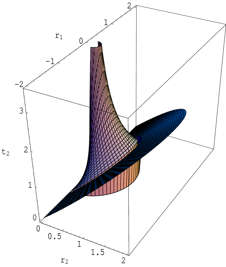
Figure 2: Map of the prefered boundary conditions in $c=2$ moduli space. The hyper plane $\rho_{2}=\tau_{2}$ is denoted in black. The grey figure below, marked by the vertical lines, is the cylinder $\rho_{1}^{2}+\rho_{2}^{2}=1/4$. The curved surface above is the hypersurface $\rho_{1}^{2}+\rho_{2}^{2}=\rho_{2}/4\tau_{2}$. In the region between the hypersurface and the hyperplane the least value for the entropy is provided by $g_{DN}$, between the cylinder and the hyperplane by $g_{DD}$, and inside of the cylinder and below the hypersurface by $g_{NN}$.

6 Acknowledgements

We thank Christoph Schweigert for discussions. The work of E. R. is partially supported by the Israel Academy of Sciences and Humanities–Centers of Excellence Programme, and the American-Israel Bi-National Science Foundation. The work of S.E. is supported by the Israel Academy of Sciences and Humanities–Centers of Excellence Programme.

References

- [1] A. M. Polyakov, JETP Lett. 12 (1970) 381
- [2] A. B. Zamolodchikov, JETP Lett. 43 (1986) 730
- [3] S. Elitzur, A. Giveon and E. Rabinovici, Nucl. Phys. B316 (1989) 679
- [4] E. Witten, Phys. Rev. D47 (1993) 3405, hep-th/9210065
- [5] I. Affleck and A. W. W. Ludwig, Phys. Rev. Lett. 67 (1991) 161
- [6] I. Affleck and A. W. W. Ludwig, Phys. Rev. B48 (1993) 7297
- [7] P. Fendley, H. Saleur and N. P. Warner, Nucl. Phys. B430 (1994) 577, hep-th/9406125
- [8] C. G. Callan and I. Klebanov, Nucl. Phys. B465 (1996) 473, hep-th/9511173
- [9] C. Schmidhuber, Nucl. Phys. B467 (1996) 146, hep-th/9601003
- [10] P.Ginsparg, Nucl. Phys B295 [FS21] (1988) 153-170
- [11] S. Elitzur, E. Gross, E. Rabinovici and N. Seiberg, Nucl. Phys. B283 (1987) 413
- [12] J.Cardy, Nucl. Phys. B324 (1989) 581
- [13] M. B. Green, Phys. Lett. B266 (1991) 325
- [14] I. Affleck and M. Oshikawa, Nucl. Phys. B495 (1997) 533, cond-mat/9612187
- [15] D. C. Lewellen, Nucl. Phys. B392 (1993) 137, hep-th/9110026
- [16] M. B. Green and M. Gutperle, Nucl. Phys. B460 (1996) 77, hep-th/9509171
- [17] J. Polchinski, TASI Lectures on D-Branes, preprint NSF-ITP-96-145, hep-th/9611050
- [18] K. S. Narain, M. H. Sarmadi and E. Witten, Nucl. Phys. B279 (1987) 369
- [19] D. Mumford, Tata lectures on Theta ( Birkhuser, Boston, 1983) p.189
- [20] A. Giveon, M. Porrati and E. Rabinovici, Phys. Rep. 244 (1994) 77