hep-th/9807098 UCLA/98/TEP/32

MIT-CTP-2756

UCSD-PTH-98-24

Field Theory Tests for Correlators

in the AdS/CFT Correspondence

Eric D’Hoker¹, Daniel Z. Freedman², and Witold Skiba³

¹Department of Physics, University of California, Los Angeles, CA 90024
^1,2Institute for Theoretical Physics,
University of California, Santa Barbara, CA 93106
²Department of Mathematics and Center for Theoretical Physics,
Massachusetts Institute of Technology, Cambridge, MA 02139
³Department of Physics, University of California at San Diego, La Jolla, CA 92093

The order $g^{2}$ radiative corrections to all 2- and 3-point correlators of the composite primary operators $\mathop{\rm Tr}X^{k}$ are computed in ${\cal N}=4$ supersymmetric Yang-Mills theory with gauge group $SU(N)$. Corrections are found to vanish for all $N$. For $k=2$ this is a consequence of known superconformal nonrenormalization theorems, and for general $k$ the result confirms an $N\rightarrow\infty$, fixed large $g^{2}N$ supergravity calculation and further conjectures in hep-th/9806074. A 3-point correlator involving ${\cal N}=4$ descendents of $\mathop{\rm Tr}X^{2}$ is calculated, and its order $g^{2}$ contribution also vanishes, giving evidence for the absence of radiative corrections in correlators of descendent operators.

1 Introduction

The Maldacena conjecture [1, 2, 3] has brought fruitful insights into string theory, supergravity (SG), and supersymmetric field theory while emphasizing a new and striking role of anti-de-Sitter space (AdS) in theoretical physics. Many correlation functions [2-14] have now been computed and compared in the boundary ${\cal N}=4$ supersymmetric Yang-Mills theory (SYM) and bulk $AdS_{5}$ SG theories. Certain 2- and 3-point correlators of operators in the same multiplet as the stress tensor and $SU(4)$ flavor currents satisfy superconformal nonrenormalization theorems [16, 15] and thus have no radiative corrections.

In a very recent paper [13] the correlators of the chiral primary family $\mathop{\rm Tr}X^{k}$ were studied. Three-point functions $\langle\mathop{\rm Tr}X^{k_{1}}\,\mathop{\rm Tr}X^{k_{2}}\,\mathop{\rm Tr}X^{k_{3}}\rangle$ of normalized operators were evaluated using an $N\rightarrow\infty$ fixed large $g^{2}N$ supergravity computation and shown to be equal to their free-field values. A conjecture was made that the correlators are independent of $\lambda=g^{2}N$ to leading order in $N$ and also a final speculation that they are independent of $g^{2}$ even for finite $N$. Known nonrenormalization theorems apply only to the case $k_{1}=k_{2}=k_{3}=2.$ Thus, these results and speculations hint at nonrenormalization properties which go beyond the known symmetries of ${\cal N}=4$ SYM theory.

In this paper, we check the nonrenormalization properties of the 2- and 3-point functions of general chiral primary operators $\mathop{\rm Tr}X^{k}$ to order $g^{2}$, by an explicit computation in the (boundary) ${\cal N}=4$ SYM theory. A further calculation of a 3-point function involving ${\cal N}=4$ descendents of the operator $\mathop{\rm Tr}X^{2}$ to the same order gives evidence that nonrenormalization also holds for descendents of the chiral primary operators.

The essential steps in the method are:

• We use an ${\cal N}=1$ description of the 6 real fields $X^{i}$ as 3 complex $z^{i}$ and their conjugates $\bar{z}^{i}$ in ${\bf 3}$ and ${\bf\bar{3}}$ representations of the manifest $SU(3)$ subgroup of the original $SU(4)$ flavor group. Without loss of generality, a choice of highest weight operators in the rank $k$ symmetric tensor representations of $SU(3)$ is made, which simplifies the flavor combinatorics.

• The essential part of the problem is then reduced to that of color combinatorics which we handle by summing over all permutations of color generators in traces. Within each such permutation of $z^{i}$-lines we sum over choices of pairs of lines carrying interaction vertices and choices of lines carrying self-energy insertions.

• In Section 2, we apply these steps to $\langle\mathop{\rm Tr}X^{k}\,\mathop{\rm Tr}X^{k}\rangle$ and show that the sum of all interactions gives an order $g^{2}$ amplitude proportional to that for the case $k=2$ which vanishes by a known nonrenormalization theorem.

• In Section 3, we study the combinatorics of the 3-point function $\langle\mathop{\rm Tr}X^{k}\,\mathop{\rm Tr}X^{k}\,\mathop{\rm Tr}X^{2}\rangle$. The net sum of interactions produces amplitudes which again vanish by nonrenormalization theorems for $k=2$.

• The analysis of the general 3-point correlator $\langle\mathop{\rm Tr}X^{k_{1}}\,\mathop{\rm Tr}X^{k_{2}}\,\mathop{\rm Tr}X^{k_{3}}\rangle$ is somewhat more involved and is presented in Sec 4.

Specifically, our results are as follows. The free field contributions to the above correlators are polynomials in $N$ of leading order $N^{k}$ for 2-point functions and order $N^{(k_{1}+k_{2}+k_{3})/2-1}$ for 3-point functions. The cancellations of radiative corrections that we find to order $g^{2}$ occur for all $N$, not just leading order. Therefore, we confirm the results and speculations of [13] in their strongest form. Concretely, the origin of the cancellations to order $g^{2}$ may be traced back to the fact that only interactions which involve at most two $X$-lines appear, so that nonrenormalization theorems for $k=2$ can be used in the proof for general values of $k$. To order $g^{4}$ however, there are also interactions involving three $X$-lines, and the situation is far more complicated. There may exist special symmetries or properties of the ${\cal N}=4$ theory which lead to nonrenormalization theorems in higher order, but the only present evidence is the large $N$ calculations of [13].

Another question of interest within the ${\cal N}=4$ SYM theory is whether the absence of radiative corrections for 2- and 3-point functions of $\mathop{\rm Tr}X^{k}$ established by nonrenormalization theorems for $k=2$ or by calculation for general $k$ remains true for all supersymmetric partners (descendents) of these operators. The case $k=2$ is of special interest because the multiplet of descendents includes the $SU(4)$ flavor currents and the stress tensor. In this case the formalism of  [17] predicts that there is a unique ${\cal N}=4$ superconformal correlator for this multiplet, so that radiative corrections of descendents should vanish as well. To check this we note that the second descendent of $\mathop{\rm Tr}X^{2}$ has the schematic form $S^{ij}=\mathop{\rm Tr}\lambda^{i}\lambda^{j}+g(\mathop{\rm Tr}X^{3})^{ij}$, where $\mathop{\rm Tr}X^{2}$ transforms in the ${\bf 20^{\prime}}$ of $SU(4)$ while $S^{ij}$ transforms in the ${\bf 10}$. We discuss the specific form of $S^{ij}$ in Section 5 and show that both free-field and order $g^{2}$ contributions to the correlator $\langle S^{ij}S^{kl}\mathop{\rm Tr}X^{2}\rangle$ vanish.

Although our method requires knowledge of the structure of the ${\cal N}=4$ theory only at a schematic level, we record here for reference the (Euclidean signature) Lagrangian in an ${\cal N}=1$ component notation (where $L$ and $R$ are chirality projectors):

$${\cal L}=\left[{\textstyle\frac{1}{4}}F_{\mu\nu}^{~{}~{}2}+{\textstyle\frac{1}{2}}\bar{\lambda}{D}\!\!\!\!/\lambda+\overline{D_{\mu}z^{i}}D_{\mu}z^{i}+{\textstyle\frac{1}{2}}\bar{\psi}^{i}{D}\!\!\!\!/\psi^{i}\right.\\ +i\sqrt{2}gf^{abc}(\bar{\lambda}_{a}\bar{z}_{b}^{i}L\psi_{c}^{i}-\bar{\psi}_{a}^{i}Rz_{b}^{i}\lambda_{c})-\frac{Y}{2}f^{abc}(\epsilon_{ijk}\bar{\psi}_{a}^{i}Lz_{b}^{j}\psi_{c}^{k}+\epsilon_{ijk}\bar{\psi}_{a}^{i}R\bar{z}_{b}^{j}\psi_{c}^{k})\\ \left.-{\textstyle\frac{1}{2}}g^{2}(f^{abc}\bar{z}_{b}^{i}z_{c}^{i})^{2}+\frac{Y^{2}}{4}f^{abc}f^{ade}\epsilon_{ijk}\epsilon_{ilm}z_{b}^{j}z_{c}^{k}\bar{z}_{d}^{l}\bar{z}_{e}^{m}\right]$$ (1.1)

We use separate coupling constants $g$ and $Y$ in order to distinguish interactions arising from the gauge and superpotential sectors. The relation $Y=\sqrt{2}g$ produces ${\cal N}=4$ SUSY.

2 The Correlators $\langle\mathop{\rm Tr}X^{k}\,\mathop{\rm Tr}X^{k}\rangle$

Without loss of generality, we may choose to evaluate the correlators of the $SU(3)$ flavor highest weight field $z^{1}$ and its complex conjugate $\bar{z}^{1}$ only. This choice vastly simplifies the problem since flavor combinatorics becomes trivial and separates from color combinatorics. We therefore study the correlator $\langle\mathop{\rm Tr}(z^{1})^{k}\,\mathop{\rm Tr}(\bar{z}^{1})^{k}\rangle$ for which contributing Feynman diagrams are shown in Fig. 1 and 2. The free field contribution is a sum over permutations of ordering in the second operator trace relative to a fixed ordering in the first operator trace,

$$\langle\mathop{\rm Tr}(z^{1})^{k}(x)\,\mathop{\rm Tr}(\bar{z}^{1})^{k}(y)\rangle =G(x,y)^{k}P_{k,k,0}(N)$$

$$P_{k,k,0}(N) \equiv\sum_{{\rm perms}\,\,\sigma}\!\!\mathop{\rm Tr}\left(T^{a_{1}}\cdots T^{a_{k}}\right)\,\mathop{\rm Tr}\left(T^{a_{\sigma(1)}}\cdots T^{a_{\sigma(k)}}\right)$$ (2.1)

where $G(x,y)=1/[4\pi^{2}(x-y)^{2}]$ is the free scalar propagator, and the sum in the second line is over all permutations $\sigma$. The permutation sum of contracted traces defines the polynomial in $N$ we have called $P_{k,k,0}(N)$. By cyclicity of the trace there are $(k-1)!$ classes of permutations each with $k$ identical contributions. So $P_{k,k,0}(N)$ has an overall factor of k. The leading term comes from “reverse order permutations” ($\sigma(1)=k$, $\sigma(2)=k-1$, etc) and is of order $P_{k,k,0}(N)\sim k(N/2)^{k}$, in agreement with [13].

Figure 1: Born graph for the $\langle\mathop{\rm Tr}(z^{1})^{k}\,\mathop{\rm Tr}(\bar{z}^{1})^{k}\rangle$ correlator.

From the Lagrangian one can easily see that there are two-particle interactions inside the “rainbow” coming from gauge boson exchange and D-term quartic vertices. (F-term vertices do not contribute.) The sum of these is a basic two particle interaction of the following structure

$$=(f^{pab}f^{pa^{\prime}b^{\prime}}+f^{pab^{\prime}}f^{pa^{\prime}b})B(x,y)G(x,y)^{2}$$ (2.2)

$$B(x,y) =b_{0}+b_{1}\ln(x-y)^{2}\mu^{2}$$

where $a,a^{\prime},b,b^{\prime}$ indicate adjoint color indices. The indicated space-time dependence is the result of integrations which may be performed explicitly, but it turns out that we will not need the precise values of $b_{0},b_{1}$. Self-energy corrections to order $g^{2}$ arise from two sources : a gauge boson exchange and a fermion loop. They are represented in the figures below by a dark dot, and may be expressed as follows

$$=\delta^{aa^{\prime}}NA(x,y)G(x,y)$$ (2.3)

$$A(x,y) =a_{0}+a_{1}\ln(x-y)^{2}\mu^{2}.$$

The coefficients $a_{i},b_{i}$ are gauge dependent, but we know that the final color traced amplitude is gauge independent and that logarithms will also cancel, since the primary operators cannot have anomalous dimension.

Figure 2: Order $g^{2}$ corrections to the 2-point function.

We shall now show that the sum of the $g^{2}$ contributions to the 2-point functions of Fig.2 precisely cancel for all $N$ and all $k$. The study of the color factors is facilitated by the following identity for any set of matrices $M_{i}$ and $N$:

$$\sum_{i=1}^{n}\mathop{\rm Tr}(M_{1}\cdots[M_{i},N]\cdots M_{n})=0.$$ (2.4)

We will use this identity here and in following sections.

For each fixed permutation of final relative to initial $z$-lines we insert the two particle interaction structure Eq. 2.2 between all distinct pairs of lines. We then convert the two $f$ symbol contractions to commutators within the final trace, and obtain the expression (omitting an overall factor of $G(x,y)^{k}$ throughout)

$${\textstyle\frac{1}{4}}(-2B)\,\mathop{\rm Tr}(T^{a_{1}}\cdots T^{a_{k}})\,\sum_{i\neq j=1}^{k}\mathop{\rm Tr}\left(T^{a_{\sigma(1)}}\cdots[T^{a_{\sigma(i)}},T^{p}]\cdots[T^{a_{\sigma(j)}},T^{p}]\cdots T^{a_{\sigma(k)}}\right).$$ (2.5)

The factor of 1/4 is inserted because the expression would otherwise overcount pairs for two reasons: first by the expected factor of two for $\sum_{i\neq j}$ rather than $\sum_{i<j}$, and second since a given choice of the pair $\sigma(i),\sigma(j)$ occurs both in the fixed final trace permutation chosen and in the permutation with $\sigma(i)$ and $\sigma(j)$ interchanged. The $-$ sign appears because of the $i$’s in $[T,T]=ifT$ and the factor of 2 because the two $ff$ terms in Eq. 2.2 contribute equally.

We now use Eq. 2.4 on one of the commutators to rewrite Eq. 2.5 as

$${\textstyle\frac{1}{2}}\,B\mathop{\rm Tr}(T^{a_{1}}\cdots T^{a_{k}})\sum_{i=1}^{k}\,\mathop{\rm Tr}\left(T^{a_{\sigma(1)}}\cdots[\,[T^{a_{\sigma(i)}},T^{p}],T^{p}]\cdots T^{a_{\sigma(k)}}\right)$$

$$={\textstyle\frac{1}{2}}\,NB\mathop{\rm Tr}(T^{a_{1}}\cdots T^{a_{k}})\sum_{i=1}^{k}\,\left(\mathop{\rm Tr}T^{a_{\sigma(1)}}\cdots T^{a_{\sigma(i)}}\cdots T^{a_{\sigma(k)}}\right)$$ (2.6)

where the last equality follows since $[[\ ,T^{p}],T^{p}]$ is the Casimir operator in the adjoint representation, so that for any generator $T^{a}$ we have $[[T^{a},T^{p}],T^{p}]=NT^{a}$. The sum $\sum_{i}$ is now over $k$ identical terms and thus collapses to an overall factor $k$. The self-energy corrections also produce an obvious factor of $k$ relative to the free field form. Adding interaction and self-energy contributions, we find the following result, including the sum over all permutations $\sigma$

$${\textstyle\frac{1}{2}}kN(B+2A)\sum_{{\rm perms}\ \sigma}\!\!\mathop{\rm Tr}\left(T^{a_{1}}\cdots T^{a_{k}}\right)\,\mathop{\rm Tr}\left(T^{a_{\sigma(1)}}\cdots T^{a_{\sigma(k)}}\right).$$ (2.7)

The nonrenormalization theorem for $k=2$ implies that $B+2A=0$, and this is enough to show that radiative corrections vanish for all values of $k$ ! Note that this argument does not require the explicit expressions for $A$ and $B$.

3 The Correlators $\langle\mathop{\rm Tr}X^{k}\,\mathop{\rm Tr}X^{k}\,\mathop{\rm Tr}X^{2}\rangle$

As we noted in the previous section, flavor combinatorics is greatly simplified by considering the $SU(3)$ flavor highest weight fields for the $\mathop{\rm Tr}X^{k}$ operators and a flavor nonsinglet for the operator $\mathop{\rm Tr}X^{2}$. Without loss of generality, we therefore study the correlators $\langle\mathop{\rm Tr}(z^{1})^{k}\,\mathop{\rm Tr}(\bar{z}^{1})^{k}\,\mathop{\rm Tr}(\bar{z}tz)\rangle$, where $t$ is a diagonal $SU(3)$ generator. This choice ensures that $\mathop{\rm Tr}(\bar{z}tz)$ transforms as ${\bf 8}$ of $SU(3)$, which is a part of the ${\bf 20^{\prime}}$ of $SU(4)$ and does not mix with the singlet. The free field contribution to this correlator is a sum of all possible pairings of fields into free propagators

$$\langle\mathop{\rm Tr}(z^{1})^{k}(x)\,\mathop{\rm Tr}(\bar{z}^{1})^{k}(y)\,\mathop{\rm Tr}(\bar{z}tz)(w)\rangle =G(x,y)^{k-1}G(x,w)G(y,w)P_{k,k,2}(N)t_{11}$$

$$P_{k,k,2}(N) \equiv k\!\!\sum_{{\rm perms}\ \sigma}\!\!\mathop{\rm Tr}\left(T^{a_{1}}\cdots T^{a_{k}}\right)\,\mathop{\rm Tr}\left(T^{a_{\sigma(1)}}\cdots T^{a_{\sigma(k)}}\right).$$ (3.1)

The additional factor of $k$ enters because of the distinguished line to the third vertex $\mathop{\rm Tr}(\bar{z}tz)$. This line can appear at any position in the first trace, and may then be moved to first position using cyclicity. Since $P_{k,k,2}=kP_{k,k,0}(N)$, the leading term for large $N$ is $P_{k,k,2}\sim k^{2}(N/2)^{k}$, in agreement with [13].

Explicit calculation of the order $g^{2}$ radiative corrections to Eq. 3 would not be necessary if, as might be expected [18, 19], the mathematical form of the correlation function of ${\cal N}=1$ superfields $\langle S(z_{1})\bar{S}(z_{2})J(z_{3})\rangle$ is uniquely determined by ${\cal N}=1$ superconformal symmetry as a function of the three superspace points $z_{i}=(x_{i},\theta_{i},\bar{\theta}_{i})$, $i=1,2,3$. Here $S(z)$ is a chiral operator of dimension $k$, $\bar{S}(z)$ is its anti-chiral conjugate, and $J(z)$ is a flavor current superfield containing a conserved vector flavor current $J_{\mu}(x)$ as its $\theta\bar{\theta}$ component. A unique superconformal form means that all component correlators, among them $\langle\mathop{\rm Tr}(z^{1})^{k}\,\mathop{\rm Tr}(\bar{z}^{1})^{k}\,\mathop{\rm Tr}(\bar{z}tz)\rangle$, contain a common coupling dependent factor. The same factor occurs in the 2-point function $\langle\mathop{\rm Tr}(z^{1})^{k}\,\mathop{\rm Tr}(\bar{z}^{1})^{k}\rangle$ because of the Ward identity, and its order $g^{2}$ term would then be absent by the calculation of Sec 2. However, current understanding of superconformal correlators is still tentative, and we will therefore present an explicit calculation of the radiative corrections to $\langle\mathop{\rm Tr}X^{k}\,\mathop{\rm Tr}X^{k}\,\mathop{\rm Tr}X^{2}\rangle$.

Previously described order $g^{2}$ interactions that contribute to the 2-point function naturally appear in the computation of the corrections to the 3-point function. In addition, there is an interaction that depends on all three space-time coordinates, which is of the form

$$\mbox{\raisebox{-12.80365pt}{\epsfbox{eq3.2.eps} }}=(f^{pab}f^{pa^{\prime}b^{\prime}}+f^{pab^{\prime}}f^{pa^{\prime}b})C(x;y,w)G(x,y)G(x,w).$$ (3.2)

Again, the specific functional form of $C$ will not be needed in the argument below.

Figure 3: Order $g^{2}$ corrections to the 3-point function. In addition to gauge boson exchange diagrams (b), (c), and (d) there are analogous diagrams with quartic interactions.

We now analyze combinatorics and color factors present in different diagrams depicted in Fig. 3. The contribution of the self-energy diagrams is straightforward to evaluate. The sum of all such diagrams is

$$N\left[(k-1)A(x,y)+A(x,w)+A(y,w)\right]$$ (3.3)

where we indicated the space-time arguments of the function $A$ defined in Eq. 2.3. As usual, we omit the part proportional to the Born contribution, which is identical for all diagrams.

Next we consider the insertion of the basic interaction 2.2 within the “rainbow” part of the correlator, as in the diagram of Fig. 3(b). We proceed as in Section 2 and insert the color factor into all pairs of lines $i,j$ that belong to the “rainbow”, and we replace the $f$ symbols with commutators inside the second trace $\mathop{\rm Tr}(T^{a_{\sigma(1)}}\cdots T^{a_{\sigma(k)}})$ in Eq. 3. We choose the index of the line to the lower vertex to be $a_{1}$ in the first trace and $a_{\sigma(k)}$ in the second, so we sum over $i\neq j=1,...,k-1$. The sum over the “rainbow” lines is

$$-{\textstyle\frac{1}{2}} \sum_{i\neq j=1}^{k-1}\mathop{\rm Tr}(T^{a_{\sigma(1)}}\cdots[T^{a_{\sigma(i)}},T^{p}]\cdots[T^{a_{\sigma(j)}},T^{p}]\cdots T^{a_{\sigma(k)}})$$

$$={\textstyle\frac{1}{2}}\sum_{i=1}^{k-1}\mathop{\rm Tr}(T^{a_{\sigma(1)}}\cdots[[T^{a_{\sigma(i)}},T^{p}],T^{p}]\cdots T^{a_{\sigma(k)}})$$

$$\qquad{}+{\textstyle\frac{1}{2}}\sum_{i=1}^{k-1}\mathop{\rm Tr}(T^{a_{\sigma(1)}}\cdots[T^{a_{\sigma(i)}},T^{p}]\cdots[T^{a_{\sigma(k)}},T^{p}])$$ (3.4)

where we have used Eq. 2.4. Using this in the second term as well as the identity $[[T^{a},T^{p}],T^{p}]=NT^{a}$, we can express the above equation as

$${\textstyle\frac{1}{2}}(k-1)N\,\mathop{\rm Tr}(T^{a_{\sigma(1)}}\cdots T^{a_{\sigma(k)}})-{\textstyle\frac{1}{2}}\,\mathop{\rm Tr}(T^{a_{\sigma(1)}}\cdots[[T^{a_{\sigma(k)}},T^{p}],T^{p}])$$

$$={\textstyle\frac{1}{2}}(k-2)N\,\mathop{\rm Tr}(T^{a_{\sigma(1)}}\cdots T^{a_{\sigma(k)}}).$$ (3.5)

The last result has the same color factor as the Born term. After contracting with the trace for the vertex at $x$, and summing over permutations, one finds the previous color polynomial $P_{k,k,2}(N)$. Therefore this set of diagrams yields

$${\textstyle\frac{1}{2}}(k-2)NB(x,y)P_{k,k,2}(N).$$ (3.6)

The remaining order $g^{2}$ diagrams are obtained by inserting the interaction of Eq. 3.2 into the Born graph. The algebra is quite similar to the previous case. We first analyze diagrams depicted in Fig. 3(c). The color structure of the diagrams with gauge boson exchange between the single leg and the “rainbow” and their analogs with $D$-term quartic interactions is again obtained by replacing the $f$ symbols with commutators inside the second trace. One of the commutators is attached to the distinguished line with the index $a_{\sigma(k)}$, the other corresponds to a line from the “rainbow” $a_{\sigma(i)}$ with $i=1,\ldots,k-1$:

$$-{\textstyle\frac{1}{2}}\sum_{i=1}^{k-1} \mathop{\rm Tr}(T^{a_{\sigma(1)}}\cdots[T^{a_{\sigma(i)}},T^{p}]\cdots[T^{a_{\sigma(k)}},T^{p}])$$

$$={\textstyle\frac{1}{2}}\,\mathop{\rm Tr}(T^{a_{\sigma(1)}}\cdots[[T^{a_{\sigma(k)}},T^{p}],T^{p}])$$

$$={\textstyle\frac{1}{2}}\,N\mathop{\rm Tr}(T^{a_{\sigma(1)}}\cdots T^{a_{\sigma(k)}}).$$ (3.7)

Again, the final result is proportional to the Born graph thus the sum over all permutations is trivial. Both gluon exchange and quartic interactions from the D-term contribute to the diagrams of Fig. 3(c). Adding the diagrams obtained by symmetrizing in $x,y$, we obtain the result

$$2N[C(x;y,w)+C(y;x,w)]P_{k,k,2}(N).$$ (3.8)

The diagram depicted in Fig. 3(d) needs to be treated separately, because quartic interactions which contribute in this case come from both the D-term and the F-term. We denote the space-time function associated with the sum of gauge boson and quartic vertices by $C^{\prime}(w;x,y)$. This is defined so that $C^{\prime}$ and $C$ would coincide if F-term vertices are excluded. All contributions to the diagram have the color factor $N$ from a double contraction on $ff$ and matrix element $t^{11}$ as a flavor factor. The latter is included in the Born amplitude (3). It is now straightforward to see that the net contribution of the graph 3(d) is

$$-2NC^{\prime}(w;x,y)P_{k,k,2}(N).$$ (3.9)

The nonrenormalization theorem for a 3-point function with $k=2$ implies that

$$N\,\bigl{[}A(x,y)+A(x,w)+A(y,w)+2C(x;y,w)+2C(y;x,w)-2C^{\prime}(w;x,y)\bigr{]}=0.$$ (3.10)

We now combine this result with the relation $A+{\textstyle\frac{1}{2}}B=0$, obtained from the nonrenormalization of the 2-point function in the previous section to show that there are no order $g^{2}$ corrections to the $\langle\mathop{\rm Tr}X^{k}\,\mathop{\rm Tr}X^{k}\,\mathop{\rm Tr}X^{2}\rangle$ correlator. Specifically the sum of all interaction diagrams computed in (3.3), (3.6), (3.8), and (3.9) is the Born term (3) multiplied by (3)

$$N \Bigl{[}(k-1)A(x,y)+A(x,w)+A(y,w)+{\textstyle\frac{1}{2}}(k-2)B(x,y)$$

$$\qquad{}{}+2C(x;y,w)+2C(y;x,w)-2C^{\prime}(w;x,y)\Bigr{]}$$

$$=N\Bigl{[}(A(x,y)+A(x,w)+A(y,w)+2C(x;y,w)+2C(y;x,w)-2C^{\prime}(w;x,y))$$

$$\qquad{}+(k-2)(A(x,y)+{\textstyle\frac{1}{2}}B(x,y))\Bigr{]}=0$$ (3.11)

and this vanishes by the nonrenormalization theorems for all $k$ and $N$.

4 The Correlators $\langle\mathop{\rm Tr}X^{k_{1}}\,\mathop{\rm Tr}X^{k_{2}}\,\mathop{\rm Tr}X^{k_{3}}\rangle$

In this section we show that a general 3-point function of $\mathop{\rm Tr}X^{k}$ does not receive corrections at order $g^{2}$. The basic ingredients of our arguments were outlined in two previous sections, but the algebra is more complicated for the case at hand. We first define the symmetric trace as follows

$$\mathop{\rm Str}(T^{a_{1}}\cdots T^{a_{k}})\equiv\sum_{{\rm perms}\ \sigma}\frac{1}{k!}\mathop{\rm Tr}(T^{a_{\sigma(1)}}\cdots T^{a_{\sigma(k)}}).$$ (4.1)

The Born diagram for the correlator $\langle\mathop{\rm Tr}X^{k_{1}}\mathop{\rm Tr}X^{k_{2}}\mathop{\rm Tr}X^{k_{3}}\rangle$ contains $\alpha_{3}=(k_{1}+k_{2}-k_{3})/2$ lines connecting the operators $\mathop{\rm Tr}X^{k_{1}}$ and $\mathop{\rm Tr}X^{k_{2}}$, etc. It is convenient and sufficiently general to work with highest weight components of the first two operators and to choose the third operator

$$\mathop{\rm Tr}(\bar{z}tz)^{\alpha_{1}\alpha_{2}}=t_{i_{1}\cdots i_{\alpha_{1}};j_{1}\cdots j_{\alpha_{2}}}\mathop{\rm Str}(\bar{z}^{i_{1}}\cdots\bar{z}^{i_{\alpha_{1}}}z^{j_{1}}\cdots z^{j_{\alpha_{2}}})$$

where $t$ is any tensor which is symmetric in its $i$ and $j$ indices and traceless upon contraction of an $i$ and $j$ index. This ensures that the operator belongs to an irreducible SU(3) component of $\mathop{\rm Tr}X^{k_{3}}$, with $k_{3}=\alpha_{1}+\alpha_{2}$.

The free field contribution to the correlator we study is then

$$\langle\mathop{\rm Tr}(z^{1})^{k_{1}}(x)\mathop{\rm Tr}(\bar{z}^{1})^{k_{2}}(y)\mathop{\rm Tr}(\bar{z}tz)^{\alpha_{1}\alpha_{2}}(w)\rangle=G(x,y)^{\alpha_{3}}G(y,w)^{\alpha_{1}}G(w,x)^{\alpha_{2}}P_{k_{1},k_{2},k_{3}}(N)t_{1\cdots 1;1\cdots 1}$$

$$\begin{aligned} P_{k_{1},k_{2},k_{3}}(N)&=\frac{k_{1}!k_{2}!}{\alpha_{3}!}\mathop{\rm Str}(T^{a_{1}}\cdots T^{a_{\alpha_{3}}}T^{b_{1}}\cdots T^{b_{\alpha_{2}}})\\ &\qquad{}\cdot\mathop{\rm Str}(T^{b_{1}}\cdots T^{b_{\alpha_{2}}}T^{c_{1}}\cdots T^{c_{\alpha_{1}}})\mathop{\rm Str}(T^{c_{1}}\cdots T^{c_{\alpha_{1}}}T^{a_{1}}\cdots T^{a_{\alpha_{3}}})\end{aligned}$$

There are three classes of diagrams contributing at order $g^{2}$ to the correlator. These are self-energy insertions described in Eq. 2.3, gauge boson exchanges within each “rainbow” (Eq. 2.2) and gauge boson exchanges from one “rainbow” to another (Eq. 3.2). The self-energy graphs are straightforward to evaluate. The sum of all such diagrams equals to

$$N\left[\alpha_{3}A(x,y)+\alpha_{2}A(x,w)+\alpha_{1}A(y,w)\right]P_{k_{1},k_{2},k_{3}}(N),$$ (4.2)

where we omitted the propagator and flavor matrix factors of the Born amplitude.

As the next step we evaluate diagrams with the insertions of the gauge boson and $D$-term quartic interactions described in Eq. 3.2 between different “rainbows.”. The color structure of these diagrams is

$$\sum_{i=1}^{\alpha_{3}}\sum_{j=1}^{\alpha_{2}}(f^{pc_{i}c^{\prime}_{i}}f^{pb_{j}b^{\prime}_{j}}+f^{pc_{i}b^{\prime}_{j}}f^{pb_{j}c^{\prime}_{i}})\Big{\{}\mathop{\rm Str}(T^{c_{1}}\cdots T^{c^{\prime}_{i}}\cdots T^{c_{\alpha_{3}}}T^{b_{1}}\cdots T^{b^{\prime}_{j}}\cdots T^{b_{\alpha_{2}}})$$

$$\qquad{}\cdot\mathop{\rm Str}(T^{b_{1}}\cdots T^{b_{\alpha_{2}}}T^{a_{1}}\cdots T^{a_{\alpha_{1}}})\,\mathop{\rm Str}(T^{a_{1}}\cdots T^{a_{\alpha_{1}}}T^{c_{1}}\cdots T^{c_{\alpha_{3}}})\Big{\}}$$

$$=-2\sum_{i=1}^{\alpha_{3}}\sum_{j=1}^{\alpha_{2}}\mathop{\rm Str}(T^{c_{1}}\cdots[T^{c_{i}},T^{p}]\cdots T^{c_{\alpha_{3}}}T^{b_{1}}\cdots[T^{b_{j}},T^{p}]\cdots T^{b_{\alpha_{2}}})$$

$$\qquad{}\cdot\mathop{\rm Str}(T^{b_{1}}\cdots T^{b_{\alpha_{2}}}T^{a_{1}}\cdots T^{a_{\alpha_{1}}})\,\mathop{\rm Str}(T^{a_{1}}\cdots T^{a_{\alpha_{1}}}T^{c_{1}}\cdots T^{c_{\alpha_{3}}}).$$ (4.3)

We will now show that the color structure arising from insertions of the $f$ symbols on any pairs of indices is identical.

$$\sum_{i=1}^{\alpha_{3}}\sum_{j=1}^{\alpha_{2}} \mathop{\rm Str}(T^{c_{1}}\cdots[T^{c_{i}},T^{p}]\cdots T^{c_{\alpha_{3}}}T^{b_{1}}\cdots[T^{b_{j}},T^{p}]\cdots T^{b_{\alpha_{2}}})$$

$$\qquad{}\cdot\mathop{\rm Str}(T^{b_{1}}\cdots T^{b_{\alpha_{2}}}T^{a_{1}}\cdots T^{a_{\alpha_{1}}})\,\mathop{\rm Str}(T^{a_{1}}\cdots T^{a_{\alpha_{1}}}T^{c_{1}}\cdots T^{c_{\alpha_{3}}})$$

$$=\mathop{\rm Str}(T^{c_{1}}\cdots T^{c_{\alpha_{3}}}T^{b_{1}}\cdots T^{b_{\alpha_{2}}})\sum_{j=1}^{\alpha_{2}}\mathop{\rm Str}(T^{b_{1}}\cdots[T^{b_{j}},T^{p}]\cdots T^{b_{\alpha_{2}}}T^{a_{1}}\cdots T^{a_{\alpha_{1}}})$$

$$\qquad{}\cdot\sum_{i=1}^{\alpha_{3}}\mathop{\rm Str}(T^{c_{1}}\cdots T^{c_{\alpha_{1}}}T^{c_{1}}\cdots[T^{c_{i}},T^{p}]\cdots T^{c_{\alpha_{3}}})$$

$$=-\mathop{\rm Str}(T^{c_{1}}\cdots T^{c_{\alpha_{3}}}T^{b_{1}}\cdots\cdots T^{b_{\alpha_{2}}})\sum_{k=1}^{\alpha_{1}}\mathop{\rm Str}(T^{b_{1}}\cdots T^{b_{\alpha_{2}}}T^{a_{1}}\cdots[T^{a_{k}},T^{p}]\cdots T^{a_{\alpha_{1}}})$$

$$\qquad{}\cdot\sum_{i=1}^{\alpha_{3}}\mathop{\rm Str}(T^{a_{1}}\cdots T^{a_{\alpha_{1}}}T^{c_{1}}\cdots[T^{c_{i}},T^{p}]\cdots T^{c_{\alpha_{3}}})$$

$$=\mathop{\rm Str}(T^{c_{1}}\cdots T^{c_{\alpha_{3}}}T^{b_{1}}\cdots\cdots T^{b_{\alpha_{2}}})\,\mathop{\rm Str}(T^{b_{1}}\cdots T^{b_{\alpha_{2}}}T^{a_{1}}\cdots T^{a_{\alpha_{1}}})$$

$$\qquad{}\cdot\sum_{i=1}^{\alpha_{3}}\sum_{k=1}^{\alpha_{1}}\mathop{\rm Str}(T^{a_{1}}\cdots[T^{a_{k}},T^{p}]\cdots T^{a_{\alpha_{1}}}T^{c_{1}}\cdots[T^{c_{i}},T^{p}]\cdots T^{c_{\alpha_{3}}}).$$ (4.4)

Using this last result we may now define the above quantity as a function $W_{k_{1},k_{2},k_{3}}(N)$, which is independent of the location of insertion of the two commutators. Adding all three sets of diagrams with interactions among two different “rainbows”, we obtain

$$-2W_{k_{1},k_{2},k_{3}}(N)\left[C(x;y,w)+C(y;x,w)-C(w;x,y)\right],$$ (4.5)

since the color factors are identical for the contributions associated with each of the three vertices, except for a sign at the $\mathop{\rm Tr}X^{k_{3}}$ vertex because the operator contains both $z$ and $\bar{z}$ fields.

The next step is the evaluation of diagrams with gauge boson exchanges within one “rainbow”. The color structure of such diagrams is of the form

$$-{\textstyle\frac{1}{2}}\sum_{i\neq j=1}^{\alpha_{2}} \mathop{\rm Str}(T^{c_{1}}\cdots T^{c_{\alpha_{3}}}T^{b_{1}}\cdots[T^{b_{i}},T^{p}]\cdots[T^{b_{j}},T^{p}]\cdots T^{b_{\alpha_{2}}})\,\mathop{\rm Str}(\cdots)\,\mathop{\rm Str}(\cdots)$$

$$={\textstyle\frac{1}{2}}\Bigl{\{}\sum_{i=1}^{\alpha_{3}}\sum_{j=1}^{\alpha_{2}}\mathop{\rm Str}(T^{a_{1}}\cdots[T^{a_{i}},T^{p}]\cdots T^{a_{\alpha_{3}}}T^{b_{1}}\cdots[T^{b_{j}},T^{p}]\cdots T^{b_{\alpha_{2}}})$$

$$\qquad{}+\sum_{j=1}^{\alpha_{2}}\mathop{\rm Str}(T^{a_{1}}\cdots T^{a_{\alpha_{3}}}T^{b_{1}}\cdots[[T^{b_{j}},T^{p}],T^{p}]\cdots T^{b_{\alpha_{2}}})\Bigr{\}}\,\mathop{\rm Str}(\cdots)\,\mathop{\rm Str}(\cdots)$$

$$={\textstyle\frac{1}{2}}W_{k_{1},k_{2},k_{3}}(N)+{\textstyle\frac{1}{2}}N\alpha_{2}P_{k_{1},k_{2},k_{3}}(N).$$ (4.6)

Finally, we evaluate the contribution of the quartic $F$-term vertex in the Lagrangian  1.1. There are nonvanishing Wick-contractions with one $z$ and one $\bar{z}$ field of the operator $\mathop{\rm Tr}X^{k_{3}}$, and one line is attached to each of the two other vertices. One can see by contracting the $\epsilon$ symbols in the F-term of  1.1, using the tracelessness of $t$, that this contribution also has the flavor factor $t_{1\cdots 1;1\cdots 1}$, The space-time function associated with the F-term will combine with gauge boson and D-term contributions at the $\mathop{\rm Tr}X^{k_{3}}$ vertex to give the same function $C^{\prime}(w;x,y)$ used in our discussion of the $k-k-2$ correlator in section 3. It remains to determine the color structure of this contribution, which is again obtained from the quartic Lagrangian vertex. The result is

$${\textstyle\frac{1}{2}}\sum_{i=1}^{\alpha_{1}}\sum_{j=1}^{\alpha_{2}}\mathop{\rm Str}(T^{a_{1}}\cdots T^{a_{i}}\cdots T^{a_{\alpha_{1}}}T^{b_{1}}\cdots T^{b_{j}}\cdots T^{b_{\alpha_{2}}})f^{pa_{i}^{\prime}b_{j}}f^{pb_{j}^{\prime}a_{i}}$$

$$\mathop{\rm Str}(T^{c_{1}}\cdots T^{c_{\alpha_{3}}}T^{b_{1}}\cdots T^{b^{\prime}_{j}}\cdots T^{\alpha_{2}})\mathop{\rm Str}(T^{c_{1}}\cdots T^{\alpha_{3}}T^{a_{1}}\cdots T^{a^{\prime}_{i}}\cdots T^{\alpha_{1}})$$ (4.7)

Replacing $f^{pa_{i}^{\prime}b_{j}}T^{b_{j}}=-i[T^{p},T^{a_{i}^{\prime}}]$ and $f^{pb_{j}^{\prime}a_{i}}T^{a_{i}}=-i[T^{p},T^{b_{j}^{\prime}}]$, we recognize this double sum as proportional to the quantity $W_{k_{1},k_{2},k_{3}}(N)$, introduced earlier.

We can now combine all contributions together to obtain

$$N\Bigl{[}\alpha_{3}(A+{\textstyle\frac{1}{2}}B)(x,y)+\alpha_{2}(A+{\textstyle\frac{1}{2}}B)(x,w)+\alpha_{1}(A+{\textstyle\frac{1}{2}}B)(y,w)\Bigr{]}P_{k_{1},k_{2},k_{3}}(N)$$

$$-\Bigl{[}2\Bigl{(}C(x;y,w)+C(y;x,w)-C^{\prime}(w;x,y)\Bigr{)}-{\textstyle\frac{1}{2}}\Bigl{(}B(x,y)-B(x,w)-B(y,w)\Bigr{)}\Bigr{]}W_{k_{1},k_{2},k_{3}}(N).$$ (4.8)

This can be seen to vanish when the nonrenormalization theorems used in previous sections are applied, specifically when $A+{\textstyle\frac{1}{2}}B=0$ is combined with Eq. 3. This result shows that order $g^{2}$ corrections cancel for arbitrary $N$ in all 3-point functions of the operators $\mathop{\rm Tr}X^{k}$.

5 A descendent correlator

It is commonly believed that the 3-point correlators of chiral primary operators determine those of descendents. For ${\cal N}=1$ SUSY the form of superconformal correlators has been discussed by [20, 18, 19]. If there is a unique super-conformal “tensor” form for a given superfield correlator, then the correlation functions of all components are determined. For ${\cal N}=4$ SUSY no off-shell superspace (or auxiliary field) formalism is known, but there is an on-shell formalism [17] which predicts a unique 3-point supercorrelator for the multiplet containing the primary $\mathop{\rm Tr}X^{2}$ and descendents. Other useful results have been deduced within this formalism [21], but the rules of applicability are not completely clear (at least to us), so it is desirable to check its predictions. Absence of radiative corrections is known for the 3-point function of flavor currents [6] and for the stress tensor [22], and we shall study here an amplitude involving the second descendent of $\mathop{\rm Tr}X^{2}$.

We shall discuss this descendent from an ${\cal N}=1$ viewpoint. For a chiral multiplet $(z,L\psi,F)$, where $\psi$ is a Majorana spinor and $L$ is the left chiral projector, the second descendent of $z^{2}$ is the operator $S=\bar{\psi}L\psi-2zF$. For the Lagrangian (1.1) the ${\cal N}=1$ auxiliary fields are $F_{i}^{a}={\textstyle\frac{1}{2}}Yf^{abc}\epsilon_{ijk}z^{j}_{b}z^{k}_{c}$. This defines the descendent operator

$$S^{ij}=\bar{\psi}^{i}_{a}L\psi^{j}_{a}-{\textstyle\frac{1}{2}}Yf^{abc}\epsilon^{mn\{i}z_{a}^{j\}}\bar{z}^{m}_{b}\bar{z}^{n}_{c}$$ (5.1)

which transforms in the ${\bf 6}$ representation of $SU(3)$ flavor, which is contained in the decomposition of the ${\bf 10}$ of $SU(4)$, whose components can be denoted by $S^{ij},i,j=1,\ldots,4$. We will study the correlator $\langle S^{ij}S^{kl}\mathop{\rm Tr}X^{2}\rangle$ which vanishes in free field approximation but could have an order $g^{2}$ contribution. Indeed, there is one $SU(4)$ invariant coupling of ${\bf 10}\otimes{\bf 10}\otimes{\bf 20^{\prime}}$ representations, so to check for the absence of radiative corrections, it is sufficient to choose the convenient set of components $\langle S^{44}(x)S^{11}(y)\mathop{\rm Tr}(\bar{z}^{1}(w))^{2}\rangle$. Here, $S^{44}$ is the $SU(4)$ partner of $S^{ij}$ whose bi-fermion term is $\mathop{\rm Tr}\bar{\lambda}L\lambda$, where $\lambda$ is the gaugino of the ${\cal N}=1$ description. To find the correctly normalized tri-boson term we use the fact that the ${\bf 10}$ representation is both the symmetric second rank tensor in the $SU(4)$ description and the self-dual third rank tensor of the $SO(6)$ description of flavor. We use an $SO(6)$ Clifford algebra construction to connect these descriptions. Omitting tedious details, the result for the descendent is

$$S^{44}=\bar{\lambda}_{a}L\lambda_{a}-{\textstyle\frac{1}{3}}Yf^{abc}\epsilon_{ijk}z^{i}_{a}z^{j}_{b}z^{k}_{c}.$$ (5.2)

(Of course, to enforce ${\cal N}=4$ SUSY, we should set $Y=\sqrt{2}g$, but we postpone this until the end of the calculation.)

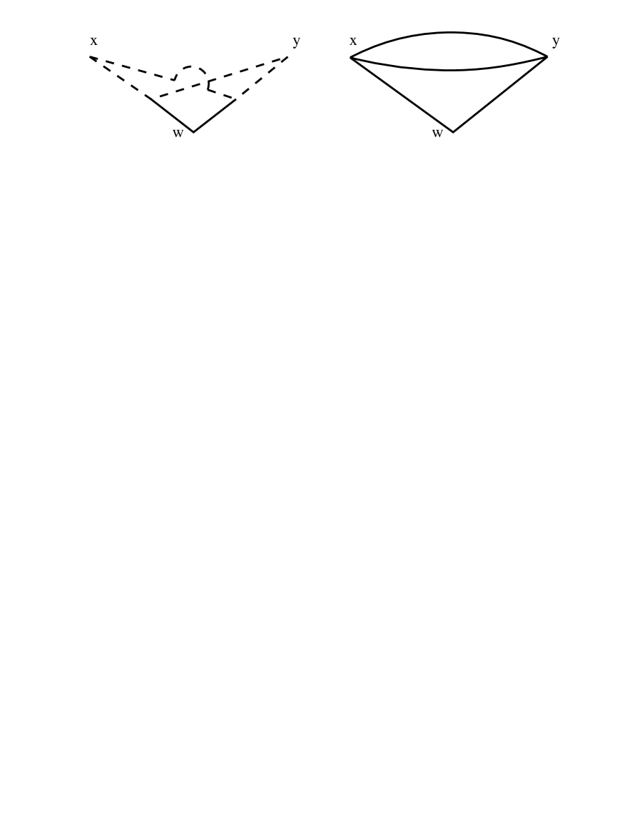
Figure 4: Two graphs contributing to the $\langle S^{44}S^{11}\mathop{\rm Tr}(\bar{z}^{1})^{2}\rangle$ correlator. Solid lines represent the boson propagators, broken ones fermion propagators.

There are two diagrams for the 2-loop correlator $\langle S^{44}(x)S^{11}(y)\mathop{\rm Tr}(\bar{z}^{1}(w))^{2}\rangle$, a nonplanar diagram with a fermion loop and a purely bosonic Born-like diagram. Diagrams are drawn in Fig. 4. The 8-dimensional integral in the nonplanar amplitude can be evaluated using the technique of conformal inversion [23, 24], and the other amplitude is elementary. Attention to combinatoric factors is essential. The results are

$${\rm nonplanar} =-g^{2}N(N^{2}-1)G(x,y)^{2}G(x,w)G(y,w)$$ (5.3)

$${\rm bosonic} ={\textstyle\frac{1}{2}}Y^{2}N(N^{2}-1)G(x,y)^{2}G(x,w)G(y,w).$$ (5.4)

We see that these two graphs cancel one another only when the ${\cal N}=4$ relation $Y=\sqrt{2}g$ is imposed, so this is clearly not a consequence of just ${\cal N}=1$ SUSY.

One should note that each graph is itself the lowest order contribution to a 3-point correlator of gauge invariant operators in the ${\cal N}=4$ SYM theory. In each amplitude only two of the three operators have scale dimension protected by R-symmetry. These correlators are thus not accessible from $AdS_{5}$ calculations with supergravity or Kaluza-Klein fields. Perhaps they can be computed using appropriate string modes and interactions.

6 Conclusions

The main result of this paper is that order $g^{2}$ radiative corrections to the correlators $\langle\mathop{\rm Tr}X^{k}\,\mathop{\rm Tr}X^{k}\rangle$ and $\langle\mathop{\rm Tr}X^{k_{1}}\,\mathop{\rm Tr}X^{k_{2}}\,\mathop{\rm Tr}X^{k_{3}}\rangle$ cancel to all orders in $N$. This confirms the $N\rightarrow\infty$ fixed large $g^{2}N$, AdS₅ supergravity calculation of Ref. [13] and the additional conjecture and speculation made in that paper concerning finite $N$ behavior. The result goes beyond known nonrenormalization theorem for 2- and 3-point functions of $\mathop{\rm Tr}X^{2}$ and thus suggests an unsuspected additional simplicity or symmetry of the ${\cal N}=4$ SYM theory.

Our method used careful combinatorics to reduce the interaction terms of general $\mathop{\rm Tr}X^{k}$ correlators to multiples of those of $\mathop{\rm Tr}X^{2}$, which vanish by nonrenormalization theorems. It seems unlikely that the method can be applied in higher order. For example in order $g^{4}$ there are interactions which involve the exchange of two gluons among three adjacent scalar lines of the “rainbow” of Fig. 1. It does seem clear, though, that the method and the order $g^{2}$ result are valid for the ${\cal N}=4$ theory with any gauge group.

The Montonen-Olive duality of ${\cal N}=4$ SYM theory relates weak and strong coupling behavior of the theory at fixed $N$. The gauge invariant correlators we study are invariant under the S-duality group so the absence of order $g^{2}$ radiative corrections for small $g$ implies that there are no order $1/g^{2}$ terms in the strong coupling expansion. This is valid for all $N$ and therefore consistent with but stronger than the conclusions of Ref. [9]. In this paper it was argued that the lowest order nonperturbative string corrections to the type IIB effective supergravity action are of order $\alpha^{\prime 3}R^{4}$ where $\alpha^{\prime}$ is the string tension and $R^{4}$ denotes a quartic contraction of the 10-dimensional curvature tensor. This correction term therefore makes no contribution to 2- and 3-point boundary correlators of the graviton and its supersymmetric partners, including Kaluza-Klein modes, in the $AdS_{5}\times S_{5}$ theory [25]. Using the Maldacena correspondence, a cubic correction of the form $\alpha^{\prime 2}R^{3}$ would produce order $1/g^{2}N$ corrections as $N\rightarrow\infty$ in the correlators $\langle\mathop{\rm Tr}X^{k_{1}}\,\mathop{\rm Tr}X^{k_{2}}\,\mathop{\rm Tr}X^{k_{3}}\rangle$.

References

• [1] J. Maldacena, β€œThe Large $N$ Limit of Superconformal Theories and Supergravity,” hep–th/9711200.
• [2] S. Gubser, I. Klebanov, and A. Polyakov, β€œGauge Theory Correlators from Non–critical String Theory,” hep–th/9802109.
• [3] E. Witten, β€œAnti–De Sitter Space and Holography,” hep–th/9802150.
• [4] M. Henningson and K. Sfetsos, β€œSpinors and the AdS/CFT correspondence,” hep-th/9803251.
• [5] W. Muck, K. Viswanathan, β€œConformal Field Theory Correlators from Classical Scalar Field Theory on $AdS_{d+1}$,” hep-th/9804035; β€œConformal Field Theory Correlators from Classical Field Theory on Anti-de Sitter Space II. Vector and Spinor Fields,” hep-th/9805145.
• [6] D. Freedman, S. Mathur, A. Matusis, and L. Rastelli, β€œCorrelation functions in the CFT(d)/AdS(d+1) correpondence,” hep-th/9804058.
• [7] H. Liu and A. Tseytlin, β€œD=4 Super Yang Mills, D=5 gauged supergravity and D=4 conformal supergravity,” hep-th/9804083.
• [8] R. Kallosh and A. Van Proeyen, β€œConformal Symmetry of Supergravities in AdS spaces,” hep-th/9804099.
• [9] T. Banks and M. Green, β€œNon-perturbative Effects in $AdS_{5}\times S_{5}$ String Theory and $d=4$ SUSY Yang-Mills,” hep-th/9804170.
• [10] G. Chalmers, H. Nastase, K. Schalm, and R. Siebelink, β€œR-Current Correlators in ${\cal N}=4$ Super Yang-Mills Theory from Anti-de Sitter Supergravity,” hep-th/9805105.
• [11] A. Ghezelbash, K. Kaviani, S. Parvizi, and A. Fatollahi, β€œInteracting Spinors-Scalars and AdS/CFT Correspondence,” hep-th/9805162.
• [12] S. Solodukhin, β€œCorrelation functions of boundary field theory from bulk Green’s functions and phases in the boundary theory,” hep-th/9806004.
• [13] S. Lee, S. Minwalla, M. Rangamani, and N. Seiberg, β€œThree-Point Functions of Chiral Operators in $D=4$, ${\cal N}=4$ SYM at Large $N$,” hep-th/9806074.
• [14] G. Arutyunov and S. Frolov, β€œOn the origin of supergravity boundary terms in the AdS/CFT correspondence,” hep-th/9806216.
• [15] S. Gubser and I. Klebanov, β€œAbsorption by Branes and Schwinger Terms in the World Volume Theory,” Phys.Β Lett. 413B, 41 (1997), hep-th/9708005.
• [16] D. Anselmi, D. Freedman, M. Grisaru, and A. Johansen, β€œNonperturbative Formulas for Central Functions of Supersymmetric Gauge Theories,” hep-th/9708042.
• [17] P. Howe and P. West, β€œSuperconformal Invariants and Extended Supersymmetry,” Phys.Β Lett. 400B, 307 (1997), hep-th/9611075.
• [18] J.-H. Park, β€œπ’©=1𝒩1{\cal N}=1 Superconformal Symmetry in Four Dimensions,” Int.Β J.Β Mod.Β Phys. A13, 1743 (1998), hep-th/9703191.
• [19] H. Osborn, to appear.
• [20] S. Gates, Jr., M. Grisaru, M. Rocek, and W. Siegel, β€œSuperspace or One Thousand and One Lessons in Supersymmetry”, Benjamin/Cummings, 1983.
• [21] S. Ferrara, C. Fronsdal, and A. Zaffaroni, β€œOn ${\cal N}=8$ Supergravity on $AdS_{5}$ and ${\cal N}=4$ Superconformal Yang-Mills theory,” hep-th/9802203.
• [22] H. Osborn, private communication.
• [23] M. Baker and K. Johnson, β€œApplications of Conformal Symmetry in Quantum Electrodynamics,” Physica 96A, 120 (1979).
• [24] J. Erlich and D. Freedman, β€œConformal Symmetry and the Chiral Anomaly,” Phys.Β Rev. D55, 6522 (1997), hep-th/9611133.
• [25] H. Kim, L. Romans, and P. van Nieuwenhuizen, β€œMass spectrum of chiral ten-dimensional N=2 supergravity on $S^{5}$,” Phys.Β Rev. D32, 389 (1985).