SU(2) Yang-Mills Theory with extended Supersymmetry in a Background Magnetic Field

Abstract

The vacuum structure of $N\!=\!2$ (and $N\!=\!4$) supersymmetric Yang-Mills theory is analyzed in detail by considering the effective potential for constant background scalar- magnetic fields within different approximations. We compare the one-loop approximation with- or without instanton improved effective coupling with the one-loop result in the dual desription. For $N\!=\!2$ we find that non-perturbative monopole degrees of freedom remove the non-trivial minima present in the (improved) one-loop potential in the strong-coupling regime. The combination of Yang-Mills and dual desription leads to a self-consistent effective potential over the full range of background fields.

I Introduction

Much attention has recently been focused on $N\!=\!2$ supersymmetric vector theories [1, 2]. A set of inequivalent vacuum states exists in these models, as the classical potential is proportional to $Tr([\phi^{*},\phi]^{2})$; distinct supersymmetric–invariant, zero–energy vacuum states are parameterized by the constant scalar component $\phi(x)$ taking its value in the Cartan subalgebra of the gauge group. In [1] it has been argued that the low energy physics of the strong-coupling regime of these theories is equivalently described by a weakly coupled dual theory. The analysis in [1] was restricted to the vacuum manifold. Attempts to generalize the duality away from the vacuum have been presented in [3, 4, 5], taking into account higher derivative terms in the effective action. In this paper, we propose another step in this direction by considering a constant Abelian background field strength and a constant scalar field, aligned in the same direction in group space. We compute the one–loop effective potential for $N\!=\!2$ and $N\!=\!4$ theories, using techniques similar to those used in [6] where the effect of an external magnetic field on the symmetry breaking patterns in a non–Abelian Higgs model was examined. For $N=4$ the one–loop effective potential should be reliable in the context of perturbation theory, as the coupling constant, once chosen to be small, is not affected by radiative corrections. In the case of $N\!=\!2$ we improve the one–loop calculation with the exact results [1], therefore including all perturbative and non-perturbative contributions up to second order in the external magnetic field.

For a given non-zero magnetic field the classical vacuum degeneracy for the scalar field is lifted by quantum corrections. More precisely, the effective potential has a relative minimum at $|\phi|^{2}/|B|=O(1)$, where $\phi$ and $B$ denote the background scalar and magnetic fields respectively. While the lifting of the classical degeneracy for the scalar field is expected, we can only determine the value of the scalar field in terms of the background magnetic field, and for $N\!=\!2$ we find that both the one–loop and the instanton improved one–loop effective potential have a minimum at a non-vanishing value of the external magnetic field for $B$. At the one–loop level $B_{min}$ is of the order of $\Lambda^{2}_{QCD}$, where the running coupling is large and the one–loop approximation therefore is not reliable. Ideally we should therefore include higher order as well as non-perturbative contributions for the higher orders in the magnetic field as well. This, of course, is beyond reach at present. However, the dual theory which should describe the the strong-coupling low energy physics of this model [1] is weakly coupled in this regime and a one–loop calculation within the dual model should be reliable. Note that the effective potential, unlike the effective action, has a physical interpretation and should therefore be duality invariant. If duality is realized for at least a small but non-vanishing magnetic field then the one-loop calculation in the dual theory should contain all relevant non-perturbative corrections in the original formulation. This is reasonable, although the duality conjecture has been proved only in the zero-energy limit [7] (see however [3, 4, 5]). We take this as motivation for the assumption that the strong-coupling effective potential be approximated by the (improved) one–loop effective potential of the dual theory which is $N\!=\!2$ supersymmetric $QED$ [1]. We find that the non-trivial minima are indeed removed by the monopole dynamics as described by the the dual action. As a result the combination of Yang-Mills- and dual description leads to to a self consistent effective potential over the full range of background fields.

In either formulation the effective potential has a non-vanishing imaginary part. While this imaginary part is normally associated with unstable (tachyonic) modes [8, 9], we can argue that they are eliminated by non-perturbative effects as in $QCD$ [10, 11, 12, 13]. In the present case, it may be interpreted as arising from monopole production in the presence of an external magnetic field.

The paper is organized as follows: In the next section we compute the one–loop effective potential for $N\!=\!2$ super Yang-Mills (SYM₂) theory for the background field configuration described above. Section three deals with the actual computation of the functional determinants arising in the one–loop computation of the effective potential and examines the vacuum structure. We repeat this for $N\!=\!4$ super Yang-Mills (SYM₄) theory in section four. In section five we improve the $N\!=\!2$ potential by including all instanton corrections to the scalar field dependence of the effective coupling. The corresponding effective potential is evaluated numerically. Next we obtain the effective potential to one–loop order in the dual theory ($N\!=\!2$ super $QED$) using the background fields dual to those above. The structure of this dual effective potential is determined numerically and compared with that of the original model. Section six contains our conclusions. The computation of the functional determinant for a general electromagnetic field is explained in the appendix.

II The N=2 Model

A harmonic superspace formulation of SYM₂ was presented in [14] where furthermore the non-renormalisation theorems for SYM₂ were revisited within that framework. For the finite contributions to the effective action we find it however easier to work in component formulation. The action is then given by

$$S = \int d^{4}x\left\{-\frac{1}{4g^{2}}F^{a}_{\mu\nu}F^{a\mu\nu}-\frac{\theta}{32\pi^{2}}F_{\mu\nu}^{a}\tilde{F}^{a\mu\nu}-(D_{\mu}\phi)^{*a}(D^{\mu}\phi)^{a}-\bar{\chi}\not{\!\!D}\chi\right.$$ (1)

$$+ \left.\frac{1}{2}g^{2}(f^{abc}\phi^{b}\phi^{*c})^{2}+\frac{ig}{\sqrt{2}}f^{abc}[\bar{\chi}^{a}\gamma_{-}\chi^{c}\phi^{b}+\bar{\chi}^{a}\gamma_{+}\chi^{c}\phi^{*b}]\right\},$$ (2)

where $\gamma_{\pm}=1\pm\gamma_{5}$, $\{\gamma_{\mu},\gamma_{\nu}\}=-2g_{\mu\nu}$ and $g_{\mu\nu}=\hbox{diag}(-+++)$ as in [15]. We take the gauge group to be $SU(2)$ and we align the background fields so that

$$\phi^{a}(x)=f\delta^{a3}+h^{a}(x)\quad\hbox{{and}}\quad A_{\mu}^{a}(x)=-\frac{1}{2}F_{\mu\nu}x^{\nu}\delta^{a3}+Q_{\mu}^{a}(x),$$ (3)

with $f$ and $F_{\mu\nu}$ constant. The gauge fixing Lagrangian is taken to be a modified version of the $R_{\xi}$ gauge [16],

$${\cal L}_{gf}=-\frac{1}{\xi g^{2}}\left[\frac{1}{2}(\partial_{\mu}Q^{\mu})^{2}+\Bigg{(}(\partial-iA)^{\nu}Q_{\nu}^{+}+ig^{2}\xi(f^{*}h^{+}+fh^{*+})\Bigg{)}\Bigg{(}(\partial+iA)^{\mu}Q_{\mu}^{-}-ig^{2}\xi(f^{*}h^{-}+fh^{*-})\Bigg{)}\right],$$ (4)

where

$$A_{\mu}=-\frac{1}{2}F_{\mu\nu}x^{\nu},\quad h^{\pm}=\frac{h^{1}\mp ih^{2}}{\sqrt{2}},\quad h^{*\pm}=\frac{h^{*1}\mp ih^{*2}}{\sqrt{2}},\quad Q=Q^{3},\quad Q^{\pm}=\frac{Q^{1}\mp iQ^{2}}{\sqrt{2}}.$$ (5)

The Faddeev–Popov ghost Lagrangian associated with this gauge fixing is, to leading order in the quantum fields when $\xi=1$,

$${\cal L}_{FP}=\bar{c_{1}}[(\partial+iA)^{2}-2g^{2}f^{*}f]c_{1}+\bar{c_{2}}[(\partial-iA)^{2}-2g^{2}f^{*}f]c_{2},$$ (6)

while the one–loop contributions arising from ${\cal L}+{\cal L}_{gf}$ are of the form

$$Q^{+}_{\mu}(\Delta^{-1})^{\mu\nu}Q^{-}_{\nu}+\left(\begin{array}[]{ll}h^{*+}&h^{+}\end{array}\right)\left(\begin{array}[]{ll}0&\Delta^{-1}_{0}\\ \Delta^{-1}_{0}&0\end{array}\right)\left(\begin{array}[]{l}h^{*-}\\ h^{-}\end{array}\right)+\left(\begin{array}[]{ll}\bar{\chi}^{+}&(\chi^{+})^{T}\end{array}\right)\left(\begin{array}[]{ll}0&\Delta_{1/2}^{-1}\\ (\Delta_{1/2}^{-1})^{T}&0\end{array}\right)\left(\begin{array}[]{l}(\bar{\chi}^{-})^{T}\\ \chi^{-}\end{array}\right),$$ (17)

where

$$\Delta^{-1}_{0}=D_{+}^{2}-M^{2},\qquad(\Delta^{-1})^{\mu\nu}=g^{\mu\nu}(D_{+}^{2}-M^{2})+2iF^{\mu\nu}\quad\hbox{{and}}\quad\Delta_{1/2}^{-1}=-i\not{\!\!D}_{+}-\frac{g}{\sqrt{2}}(\gamma_{+}f^{*}+\gamma_{-}f),$$ (18)

respectively. In (17), “T” refers to a transpose in the Dirac indices only, $D_{\pm\mu}\equiv\partial_{\mu}\pm iA_{\mu}$ and $M^{2}=2g^{2}f^{*}f$. From (6-18) it is then easy to see that the ghost and scalar loops cancel, so that

$$iW^{(1)} = -tr\ln\left[\Delta^{\mu\nu}\right]+2tr\ln\left[\Delta_{1/2}\right],$$ (19)

where, in addition to (18), we have also used the notation

$$\Delta_{1/4}=\left(D_{+}^{2}+\frac{1}{2}\sigma_{\mu\nu}F^{\mu\nu}-M^{2}\right)^{-1},\quad\sigma_{\mu\nu}\equiv\frac{i}{2}[\gamma_{\mu},\gamma_{\nu}].$$ (20)

If we now regulate the logarithm and reciprocal of operators occurring in (19) using $\zeta$–regularization [6, 17], and its generalization, operator regularization [18], then we find that for operators $H_{i}$,

$$\ln(H_{i}/\mu^{2})=-\left.\frac{d}{ds}\right|_{0}\frac{\mu^{2s}}{\Gamma(s)}\int\limits_{0}^{\infty}d(it)(it)^{s-1}e^{-iH_{i}t},$$ (21)

and

$$(H_{1}H_{2}\ldots H_{N})^{-1}=\left.\frac{d}{ds}\right|_{0}\left\{\frac{\mu^{2s}}{\Gamma(s+1)}\int\limits_{0}^{\infty}d(it_{1})(it_{1})^{s}e^{-iH_{1}t_{1}}\ldots\frac{\mu^{2s}}{\Gamma(s+1)}\int\limits_{0}^{\infty}d(it_{N})(it_{N})^{s}e^{-iH_{N}t_{N}}\right\}.$$ (22)

(23)

In (21) and (23) $\mu^{2}$ is an arbitrary dimensionful parameter.

III The Case of the Background Magnetic Field

We now specialize to the case where $F_{\mu\nu}$ corresponds to a magnetic field only, so that $F_{12}=-F_{21}=B$ (the formulae for the most general case of the electromagnetic field are given in Appendix A). As has been shown in [15, 19, 20] (see also equation (A2) with $K_{-}=B$ and $K_{+}=0$ in Appendix A), in this case we have

$$\langle x^{\prime}|\exp(iD_{+}^{2}t)|x\rangle=\frac{-i}{(4\pi t)^{2}}\frac{Bt}{\sin(Bt)}\exp\left[\frac{ix^{2}_{\parallel}}{4t}+\frac{ix^{2}_{\perp}B}{4\tan(Bt)}+\frac{iB}{2}(x_{2}x_{1}^{\prime}-x_{1}x_{2}^{\prime})\right],$$ (24)

($x^{2}_{\perp}\equiv(x_{1}-x_{1}^{\prime})^{2}+(x_{2}-x_{2}^{\prime})^{2}$, $x^{2}_{\parallel}\equiv(x_{3}-x_{3}^{\prime})^{2}-(x_{0}-x_{0}^{\prime})^{2}$).

Furthermore, since $(\sigma_{12})^{2}=1\!\!1_{4}$, it is easily shown that

$$tr\exp\left[-\frac{i}{2}\sigma_{\mu\nu}F^{\mu\nu}t\right]=4\cos(Bt),$$ (26)

and

$$tr\exp\left[-2F^{\mu\nu}t\right]=4\cos^{2}(Bt).$$ (27)

Since

$$tr\ln\left[-i\not{\!\!D}_{+}-\frac{g}{\sqrt{2}}(\gamma_{+}f^{*}+\gamma_{-}f)\right] = tr\ln\left[-i\not{\!\!D}_{+}+\frac{g}{\sqrt{2}}(\gamma_{+}f+\gamma_{-}f^{*})\right]$$ (28)

$$= \frac{1}{2}tr\ln\left[D_{+}^{2}-M^{2}+\frac{1}{2}\sigma_{\mu\nu}F^{\mu\nu}\right],$$ (29)

we find that for the leading terms in (19)

$$iW_{eff} \equiv -tr\ln\left[\Delta^{\mu\nu}\right]+2tr\ln\left[\Delta_{1/2}\right]=-tr\ln\left[\Delta^{\mu\nu}\right]+tr\ln\left[\Delta_{1/4}\right]\equiv i\int d^{4}x{\cal L}_{eff},$$ (30)

and (21) and (24)–(27) imply

$$i{\cal L}_{eff}=\left.\frac{d}{ds}\right|_{0}\frac{\mu^{2s}}{\Gamma(s)}\int\limits_{0}^{\infty}d(it)(it)^{s-1}e^{-iM^{2}t}\frac{-i}{(4\pi t)^{2}}\frac{Bt}{\sin(Bt)}[4\cos^{2}(Bt)-4\cos(Bt)].$$ (31)

Furthermore, it is possible to show using (24) (or (A2) in the case of the electromagnetic field of a general form) that

$$\int d^{4}xd^{4}x^{\prime}\langle x|e^{iD_{+}^{2}t_{1}}|x^{\prime}\rangle\langle x^{\prime}|\not{\!\!D}_{+}e^{iD_{+}^{2}t_{2}}|x\rangle=0.$$ (32)

We first note that the term in the brackets in (31) contains no term below order $t^{2}$ when expanded in powers of $t$; consequently there is no mass renormalization in the theory as expected due to the supersymmetry of the model (see also [14] and references therein).

To continue, it is convenient to rewrite ${\cal L}_{eff}$ in (31) as

$${\cal L}_{eff}=\left.\frac{d}{ds}\right|_{0}\frac{\mu^{2s}}{\Gamma(s)}\frac{1}{4\pi^{2}}\int\limits_{0}^{\infty}d(it)(it)^{s-3}e^{-iM^{2}t}\frac{Bt}{\sin(Bt)}\left[-\frac{Bt}{2}\sin(Bt)+\left(\cos^{2}(Bt)-\cos(Bt)+\frac{Bt}{2}\sin(Bt)\right)\right].$$ (33)

Initially, we compute

$$\left.\frac{d}{ds}\right|_{0}\frac{\mu^{2s}}{\Gamma(s)}\frac{1}{4\pi^{2}}\int\limits_{0}^{\infty}d(it)(it)^{s-3}e^{-iM^{2}t}\frac{Bt}{\sin(Bt)}\left[-\frac{Bt}{2}\sin(Bt)\right]=\frac{B^{2}}{8\pi^{2}}\left[-\ln\sigma-\ln\frac{|B|}{\mu^{2}}\right],$$ (34)

where $\sigma\equiv M^{2}/|B|=2g^{2}f^{*}f/|B|$. The remaining integral in (33) is free of any divergence at $s=0$, so we are left with

$${\cal L}_{eff}=-\frac{B^{2}}{4\pi^{2}}\left[\frac{1}{2}\left(\ln\sigma+\ln\frac{|B|}{\mu^{2}}\right)+\int\limits_{0}^{\infty}\frac{dt}{t^{2}}e^{-it\sigma}\left([t-\sin t]+[\tan\frac{t}{2}-\frac{t}{2}]\right)\right].$$ (35)

We first note that, using Eq.3.551.9 of [21],

$$I_{1} = \int\limits_{0}^{\infty}\frac{dt}{t^{2}}e^{-it\sigma}\left[\tan\frac{t}{2}-\frac{t}{2}\right]=\int\limits_{\sigma}^{\infty}dz\int\limits_{0}^{\infty}\frac{dt}{t}e^{-2tz}\left[\tanh t-t\right]$$ (36)

$$= \int\limits_{\sigma}^{\infty}dz\left[\ln\frac{z}{2}+2\ln\Gamma\left(\frac{z}{2}\right)-2\ln\Gamma\left(\frac{z+1}{2}\right)-\frac{1}{2z}\right].$$ (37)

Next, we get the imaginary part,

$$I_{2} = -i\int\limits_{0}^{\infty}\frac{dt}{t^{2}}\sin(t\sigma)\left[t-\sin t\right]=i\int\limits_{0}^{\infty}dt\left[\frac{\cos(1-\sigma)t-\cos(1+\sigma)t}{2t^{2}}-\frac{\sin\sigma t}{t}\right],$$ (38)

which, upon integrating the first two terms by parts and using

$$\int\limits_{0}^{\infty}dx\frac{\sin\lambda x}{x}=\frac{\pi}{2}\frac{\lambda}{|\lambda|},\quad(\lambda\neq 0)$$ (39)

becomes

$$I_{2}=-i\frac{\pi}{2}(1-\sigma)\theta(1-\sigma).$$ (40)

Lastly, we have

$$I_{3} = \int\limits_{0}^{\infty}\frac{dt}{t^{2}}\cos(t\sigma)\left[t-\sin t\right]=\int\limits_{0}^{\infty}dt\left[\frac{\cos\sigma t}{t}-\frac{\sin(1-\sigma)t+\sin(1+\sigma)t}{2t^{2}}\right],$$ (41)

which upon integrating the first term by parts becomes

$$I_{3} = -1+\lim_{\lambda\to 0}\int\limits_{\lambda}^{\infty}\frac{dt}{t^{2}}\left[\frac{\sin\sigma t}{\sigma}-\frac{\sin(1-\sigma)t+\sin(1+\sigma)t}{2}\right]$$ (43)

$$=-1+\frac{1+\sigma}{2}\ln(1+\sigma)+\frac{1-\sigma}{2}\ln|1-\sigma|-\ln\sigma.$$

Together, contributions to ${\cal L}_{eff}$ coming from (37)–(43) show that

$${\cal L}_{eff} = -g^{2}\frac{B^{2}}{4\pi^{2}}\left\{\frac{1}{2}\ln\frac{2g^{2}f^{*}f}{\mu^{2}}+U(\sigma)\right\},$$ (44)

with

$$U(\sigma) = \int\limits_{\sigma}^{\infty}dz\left[\ln\frac{z}{2}+2\ln\Gamma\left(\frac{z}{2}\right)-2\ln\Gamma\left(\frac{z+1}{2}\right)-\frac{1}{2z}\right]-\ln(\sigma)$$ (46)

$$-1+\frac{1+\sigma}{2}\ln(1+\sigma)+\frac{1-\sigma}{2}\ln|1-\sigma|-i\frac{\pi}{2}(1-\sigma)\theta(1-\sigma).$$

Including the classical contribution into the effective Lagrangian (44) and trading $\mu$ for the renormalization group invariant scale

$$\Lambda_{\zeta}^{2}=\mu^{2}e^{-\frac{4\pi^{2}}{g^{2}}},$$ (47)

we obtain

$$V_{B}=\frac{B^{2}}{8\pi^{2}}\ln\frac{2g^{2}f^{*}f}{\Lambda_{\zeta}^{2}}+\frac{B^{2}}{4\pi^{2}}U(\sigma).$$ (48)

The imaginary part of $U(\sigma)$ arises, as in pure Yang–Mills theory, due to unstable (tachyonic) modes in the spectrum of the charged vector particle in the presence of a background magnetic field [8, 9]. In [10], these modes are removed by treating their classical part of the action as a Higgs model, i.e. by taking into account the quartic self–interaction of these unstable modes non–perturbatively. An alternate treatment is given in [11] (for a review see [22]). The imaginary part of the effective action now disappears, and the real part is believed to remain unaltered. Here we must note, that this real part would quite likely be shifted though if the coupling between the stable and unstable modes were included in the discussion. But even in the case of pure Yang–Mills theory, this is a rather complicated problem which has not been rigorously solved yet. Note however that even in the case when this shift turns out to be big, one should expect that the true vacuum energy is lower then the energy of the metastable state with a non-zero imaginary part. Other discussions on the stability of translation invariant background configurations in Yang–Mills theories are given in [12, 13].

In the present model it may appear natural to associate the imaginary part with monopole production in an external magnetic field. However, perturbation theory does not “see” these degrees of freedom and therefore this interpretation is possibly too far fetched.

Let us now discuss the vacuum structure predicted by the effective potential (48). If we ignore the imaginary part in (48), we find numerically that $dReV(\sigma)/d\sigma=0$ implies that $\sigma_{min}\simeq 0.596$ and $U_{min}\simeq-0.358$. The effective potential with $\sigma$ at the minimum reads

$$V_{min}(B)=\frac{1}{2g^{2}}B^{2}\left(1+\frac{g^{2}}{4\pi^{2}}\ln\frac{|B|}{\mu^{2}}\right)+\frac{B^{2}}{4\pi^{2}}U_{min}+\frac{B^{2}}{8\pi^{2}}\ln(\sigma_{min}).$$ (49)

The existence of a negative minimum of $V_{min}(B)$ follows from the fact that $V_{min}(0)=0$, $V_{min}(B\to\infty)>0$ and for small $B$, $V_{min}(B)<0$ (because of dominance of the logarithmic term in (49)). At the minimum, the magnetic field is given by

$$B_{min}=\Lambda_{\zeta}^{2}\exp\left(-2U_{min}-\frac{1}{2}\right).$$ (50)

However, if $t\!=\!{1\over 2}\ln(M^{2}/\Lambda_{\zeta}^{2})$, then the running coupling satisfies the equation

$$\frac{\hbox{d}}{\hbox{dt}}\bar{g}(t)=-\frac{1}{2\pi^{2}}g^{3}(t),$$ (51)

so that

$$\bar{g}(t)=\frac{g^{2}}{1+g^{2}t/\pi^{2}}.$$ (52)

For $\sigma\!=\!\sigma_{min}$, $B\!=\!B_{min}$ then the value of $t\!=\!{1\over 2}\ln(\sigma_{min}B_{min}/\Lambda^{2})$ is such that by (51) the coupling $\bar{g}^{2}(t)$ is large and hence the one–loop potential is unreliable. However, for any value of the external magnetic field, the scale of the scalar field is fixed, thereby breaking the classical vacuum degeneracy completely. For large values of $B$, where $\bar{g}(t)$ is small, $V_{min}$ in (49) is positive, as expected for a supersymmetric theory.

Before seeing how the one-loop approximation can be improved upon, we turn to $N\!=\!4$ super Yang-Mills theory in the one-loop approximation.

IV The N=4 model in a background magnetic field

The effective potential for SYM₄ in a background with constant field strength has been considered in [9, 23]. As in that reference we simplify the algebra by viewing the $N\!=\!4$ supersymmetric gauge theory as an N=1 supersymmetric gauge theory in ten dimensions in which six of the dimensions have been suppressed [24]. The original vector field $A_{\alpha}^{a}$ $(\alpha=1...10)$ decomposes into a four component vector field $A_{\mu}^{a}$ $(\mu=1...4)$, three scalars, identified with $A_{5}^{a}...A_{7}^{a}$ and three pseudo-scalars $A_{8}^{a}...A_{10}^{a}$, while the original Majorana-Weyl spinor in ten dimensions becomes a set of four Majorana spinors in four dimensions. In four dimensions, the couplings of these matter fields is SU(4) invariant.

The N=1 supersymmetric gauge theory in ten dimensions that we will consider has the action

$$S=\int d^{10}x\left[-\frac{1}{4}G_{\alpha\beta}^{a}(V)G^{a\alpha\beta}(V)-\frac{i}{2}\bar{\lambda}^{a}\not{\!\!D}^{ab}\lambda^{b}\right].$$ (53)

We now use the Honerkamp gauge [25]

$$D^{ab}(A)\cdot Q^{b}=0.$$ (54)

where V has been decomposed into the sum of a background field $A_{\alpha}^{a}$ and a quantum field $Q_{\alpha}^{a}$. If the background field in four dimensions corresponds to a constant background U(1) field $F_{\mu\nu}^{a}\;(\mu,\;\nu=1...4)$ and a constant scalar field of magnitude $gv$, both in the direction $n^{a}$ in group space, then

$$A_{\mu}^{a}=-\frac{1}{2}F_{\mu\nu}\;x^{\nu}n^{a},$$ (55)

$$\sum_{\alpha=5}^{10}\;A_{\alpha}^{a}\;A^{\alpha b}=g^{2}v^{2}n^{a}\delta^{ab}\equiv M^{2}n^{a}\delta^{ab}.$$ (56)

The effective action to one-loop order is then given by

$$\exp iW^{(1)}=det\left(D^{2ab}\right)\;det^{-\frac{1}{2}}(D^{2ab}g_{\alpha\beta}+2f^{apb}F_{\alpha\beta}^{p})\;det^{\frac{1}{2}}\left(\not{\!\!D}^{ab}\left(\frac{1+\gamma_{11}}{2}\right)\right)^{2}$$ (57)

in ten dimensions (with the three terms in (57) corresponding to the contribution of the ghost, vector, and Majorana-Weyl spinor respectively); dimensionally reducing this to four dimensions with the background field satisfying the conditions of (55) and (56) converts (57) into

$$\exp iW^{(1)} = det(D^{2ab}-M^{2})\;det^{-\frac{1}{2}}\left(\left(D^{2ab}-M^{2}\right)g_{\mu\nu}-2iF_{\mu\nu}\right)$$ (59)

$$\left[det^{-\frac{1}{2}}(D^{2ab}-M^{2})\right]^{6}\;det^{\frac{1}{2}}(D^{2ab}-M^{2}+\frac{1}{2}\sigma_{\mu\nu}F^{\mu\nu}).$$

All derivatives and functional determinants in (59) are understood to be in four dimensions, all group indices have been suppressed once we set $(X)^{ab}=i\;f^{apb}(X^{p})$, $D=\partial-iA$, and $\sigma_{\mu\nu}=\frac{i}{2}[\gamma_{\mu},\gamma_{\nu}]$.

We can now proceed using the techniques outlined in the previous section. Regulating as in eq. (11) we see that

$$\left.iW^{(1)}=-\frac{d}{ds}\right|_{0}tr\frac{1}{\Gamma(s)}\int_{0}^{\infty}\;dit(it)^{s-1}\;e^{-i[-D^{2}+M^{2}]t}\;\left[-\frac{1}{2}\;e^{2F_{\mu\nu}t}\;\;-2+\frac{1}{2}\;e^{\frac{i}{2}\sigma_{\mu\nu}F^{\mu\nu}t}\right].$$ (60)

Using (13) and (14), we see that in the presence of an external magnetic field,

$$\left.iW^{(1)}=\frac{d}{ds}\right|_{0}\frac{1}{\Gamma(s)}\int_{0}^{\infty}\;d\;it(it)^{s-1}\left(-\frac{i}{(4\pi t)^{2}}\frac{Bt}{\sin Bt}\right)(4\cos^{2}Bt+4-8\cos Bt)e^{-iM^{2}t}.$$ (61)

(An overall factor of 2 comes from the trace in group space.) The integral over $t$ in (61) is free of divergences at $s=0$, and hence, upon using some trigonometric identities, we see that

$$iW^{(1)}=\frac{8B^{2}}{(4\pi)^{2}}\int_{0}^{\infty}d(it)(it)^{-2}\left[\left(\tan\frac{t}{2}-\frac{t}{2}\right)+\left(\frac{t}{2}-\frac{1}{2}\sin t\right)\right]e^{-i\sigma t},$$ (62)

where $\sigma=M^{2}/B$. The integrals in (62) are given in (22), (25) and (27) so that

$$iW^{(1)} = -\frac{iB^{2}}{2\pi^{2}}\left[\int_{\sigma}^{\infty}dz\left(\ln\frac{z}{2}+2\ln\Gamma\left(\frac{z}{2}\right)-2\ln\Gamma\left(\frac{z+1}{2}\right)-\frac{1}{2z}\right)\right.$$ (63)

$$+ \left.\frac{1}{2}\left(-1+\frac{1+\sigma}{2}\ln(1+\sigma)+\frac{1-\sigma}{2}\ln\left|1-\sigma\right|-\ln\sigma-i\frac{\pi}{2}(1-\sigma)\theta(1-\sigma)\right)\right]$$ (65)

$$\equiv-\frac{iB^{2}}{2\pi^{2}}\overline{U}(\sigma).$$

The effective potential to one-loop order is hence given by

$$V_{B}=\frac{1}{2}B^{2}\left[1+\frac{1}{\pi^{2}}\overline{U}(\sigma)\right].$$ (66)

We note in passing that the result (65) could also be obtained by identifying the mass term in [23] with the background scalar. As for the imaginary part the discussion in the last section could be repeated here. In particular for $M\to 0$ we recover the result of [23] for a vanishing scalar background.

The minimum value of ReV_B occurs when $d\left[Re\overline{U}(\sigma)\right]/d\sigma=0$; this occurs when

$$\sigma_{min}=.797$$ (67)

at which point

$$Re\overline{U}_{min}=-.247$$ (68)

so that $V_{B}>0$ at $\sigma=\sigma_{min}$, in agreement with the theorem that the vacuum energy of a supersymmetric theory is non-negative. However, for $B\neq 0$, the degeneracy in the vacuum expectation value of the scalar particle is broken by (67). This result is reliable in perturbation theory, for in $N=4$ SUSY the coupling $g$ does not run and hence may be chosen to be small irrespective of the value of B. Furthermore the non-renormalization theorem of [26] excludes further corrections to the $B^{4}$ term.

V Non-perturbative corrections

In this section we analyze the effect of non-perturbative corrections to the effective potential in two different ways. First by including all instanton corrections to the running coupling and second by evaluation the effective potential within the dual description.

A Instanton improved potential for N=2

We start by comparing (48) with the exact low energy effective action [1].

$${\cal L}_{SW}=\frac{1}{4\pi}Im\left[\int d^{4}\theta\frac{\partial{\cal F}(A)}{\partial A}\bar{A}+\int d^{2}\theta\frac{1}{2}\frac{\partial^{2}{\cal F}(A)}{\partial A^{2}}W_{\alpha}W^{\alpha}\right],$$ (69)

where $A\!=\!a+\theta\chi+\cdots$ and $W_{\alpha}\!=\!\chi_{\alpha}+\cdots$ are the $N=1$ chiral and vector multiplets, respectively. (The scalar component of $A$ is proportional to $f$ in our notation.) The function ${\cal F}(A)$ in the region of validity of perturbation theory ($|a|\to\infty$) is given by [1, 27]

$${\cal F}(A)=\frac{i}{2\pi}A^{2}\left(\ln\frac{A^{2}}{\Lambda^{2}}+c\right),$$ (70)

where $c$ depends on the renormalization scheme. Matching the scales as in [28] we get from (70) with $\Lambda^{2}_{\zeta}\!=\!\Lambda^{2}_{\overline{DR}}\!=\!{1\over 2}\Lambda^{2}$ (here $\Lambda$ corresponds to the scheme used in [1] and $\Lambda_{\overline{DR}}$ is the scale of dimensional reduction combined with minimal subtraction)

$$V_{B}\simeq\frac{B^{2}}{8\pi^{2}}\ln\frac{2|a|^{2}}{\Lambda_{\zeta}^{2}},\quad\mbox{as}\quad\frac{|a|}{\Lambda_{\zeta}}\to\infty,$$ (71)

with $c=0$. From (46) it follows that $U(\sigma)\rightarrow 0$ for $\sigma\rightarrow\infty$, so that (71) is identical with (48) if we make the identification $a\!=\!gf$. This is also the identification which is consistent with BPS mass formula $M^{2}\!=\!2|an_{e}+a_{D}n_{m}|^{2}$.

The analysis of [1] was based on the following argument: each fixed value of the scalar field $|a|$ defines a distinct vacuum of the system; different values of $|a|$ define inequivalent vacua. The reason for this (at least in the asymptotic region $|a|\to\infty$) is well understood. As is seen from (71), for any value of $|a|$ the minimum of the effective potential is achieved by taking $B=0$. Since at this minimum, the value of the potential is zero, the lowest possible in supersymmetric models, we conclude that there exist different vacua for each choice of the value of $|a|$. On the other hand, for values of $|a|$ of the order of $\Lambda$ the potential (71) is unbounded below. It was argued in [1] and later shown [7] that the function ${\cal F}(A)$ has a unique extension to the strong-coupling limit, compatible with supersymmetry and a finite number of singularities. Furthermore the quantum moduli-space is in one-to-one correspondence with the parameter $u=\hbox{tr}\langle\phi^{2}\rangle$ which takes its value in the upper half plane [7]. For large values of $a$, $u=\frac{1}{2}a^{2}$ since in this region $\phi=\frac{1}{2}a\sigma^{3}$. For $u\simeq\Lambda^{2}$ the effective coupling diverges due to the appearance of massless composite fields which are magnetic monopoles. In the neighbourhood of this singularity the theory should then be accurately described by a dual theory which is magnetic $N=2\;QED$ [1].

From the above discussion we draw the following conclusions. First of all, the one-loop result (48) can be improved by replacing the first term by the corresponding non-perturbative expression [1]. The higher loop and non-perturbative contributions to $U(\sigma)$ which are important in the regime where the scalar and/or the magnetic field are of the order of $\Lambda$, will be approximated by computing the analogue of $U(\sigma)$ in the corresponding dual model. This will be done by evaluating to one–loop order the effective potential in $N\!=\!2\;QED$ in the presence of background scalar and electromagnetic fields which are dual to the fields appearing in (48). The contribution to the analogue of the first term in (48) can be compared to the non-perturbative expression of this first term in (48), obtained by using the methods of [1]. This complements the comparison of the non-perturbative extension to the instanton contribution to the effective potential of $N\!=\!2$ $SU(2)$ super-Yang-Mills theory (see [27]). Furthermore the remaining part of the one–loop effective potential in $N\!=\!2\;QED$ should approximate the non-perturbative extension of the function $U(\sigma)$ in (48). The accuracy of this approximation relies on to what extent duality in $N\!=\!2$ Yang-Mills theory is realized away from the strict vacuum and the strong–weak coupling singularities. We therefore expect it to be good for small magnetic fields in the neighbourhood of the point where monopoles are massless, while nothing is known in the general case. We cannot test this directly as higher loop and instanton corrections to the effective potential in the presence of a background magnetic field are unknown.

Let us first implement the instanton corrections. For this we substitute the exact result [1] for the running coupling in the first term in (48), which then becomes

$$V_{B}=\frac{B^{2}}{8\pi}\hbox{Im}\left(\tau(u)\right),$$ (72)

where the explicit expression for $\tau$ and $f$ as a function of $u\!=\!\langle tr\phi^{2}\rangle$ are given by [1, 29]

$$\tau(u)=i\frac{F[1/2,1/2,1,\frac{u-1}{u+1}]}{F[1/2,1/2,1,\frac{2}{u+1}]}.$$ (73)

This is the full non-perturbative expression for the effective potential in the presence of a very weak magnetic field. Concerning the second term in (48) there appears to be an ambiguity. There are two different non-perturbative expressions for $\sigma$, each of which reduce to the perturbative expression (below (62)); both $\sigma\!=\!\frac{2|a|^{2}}{|B|}$ and the gauge-invariant form $\sigma\!=\!\frac{4u}{|B|}$ reduce to the perturbative expression. In Fig. 1 the improved effective potential is plotted for different values of $u$ (horizontal) and the magnetic field $|B|$ for both possible parametrizations of $\sigma$. This shows that the qualitative behaviour is the same for both choices. The exact relation between $u$ and $a$ is [1]

$$a(u)=\sqrt{2}\sqrt{u+1}\;F\left(-\frac{1}{2},\frac{1}{2},1,\frac{2}{1+u}\right).$$ (74)

B Dual description

The only theory with the same number of degrees of freedom as the YM-theory, which has $N\!=\!2$ SUSY and in which the coupling runs to zero at small scale is $N\!=\!2$ SUSY QED with magnetic rather than electric charges. In component form its Lagrangian reads [30]

$$S = \int d^{4}x\left\{-\frac{1}{4}F_{\mu\nu}F^{\mu\nu}-(\partial_{\mu}\phi_{D})^{*}(\partial^{\mu}\phi_{D})-\bar{\lambda}^{i}\partial\!\!\!/\lambda_{i}+{1\over 2}X^{2}\right.$$ (78)

$$\qquad\qquad-(D_{\mu}A^{i})^{*}D^{\mu}A_{i}-\bar{\psi}\not{\!\!D}\psi+|F^{i}|^{2}$$

$$\qquad\qquad-i2g\bar{\lambda}^{i}\psi\bar{A}_{i}+i\sqrt{2}g\bar{\psi}[\phi_{D}\gamma_{-}+\phi_{D}^{*}\gamma_{+}]\psi$$

$$\left.\qquad\qquad+4igX^{ij}\bar{A}_{i}A_{j}-2g^{2}|\phi_{D}|^{2}\bar{A}^{i}A_{i}\right\}.$$

The background configurations are now $\phi_{D}\!=\!f_{D}$ and $F_{D\mu\nu}$ respectively. We follow [1, 4] in order to determine $F_{D\mu\nu}$. Consider

$$S=\frac{1}{16\pi}\int\hbox{d}^{4}x\left[-\frac{4\pi}{\bar{g}^{2}}F_{\mu\nu}F^{\mu\nu}-\frac{\bar{\theta}}{2\pi}F_{\mu\nu}\tilde{F}^{\mu\nu}-4V^{\mu}\partial^{\nu}\tilde{F}_{\mu\nu}\right],$$ (79)

where $\bar{g},\bar{\theta}$ denote the effective coupling and vacuum angle, $\tilde{F}_{\mu\nu}\!=\!{1\over 2}\epsilon_{\mu\nu\lambda\sigma}F^{\lambda\sigma}$ and $V^{\mu}$ is a Lagrange multiplier vector field imposing the Bianchi identity $\partial_{\nu}\tilde{F}^{\mu\nu}\!=\!0$. Varying (79) with respect to $F_{\mu\nu}$ then leads to

$$F_{D\mu\nu}=\frac{4\pi}{\bar{g}^{2}}\tilde{F}_{\mu\nu}-\frac{\bar{\theta}}{2\pi}F_{\mu\nu},$$ (80)

where $F_{D\mu\nu}=\partial_{\mu}V_{\nu}-\partial_{\nu}V_{\mu}$ is the field strength in the dual theory. This is consistent with

$$F_{\mu\nu}=\frac{4\pi}{\bar{g}_{D}^{2}}\tilde{F}_{D\mu\nu}-\frac{\bar{\theta}_{D}}{2\pi}F_{D\mu\nu},$$ (81)

provided $\tau_{D}\!=\!\frac{\bar{\theta}_{D}}{2\pi}+\frac{i4\pi}{\bar{g}_{D}^{2}}\!=\!-\frac{1}{\tau}$. With $\epsilon_{0123}\!=\!1$ and $F_{12}\!=\!B$ we see by (80) that

$$F_{D03}=\frac{4\pi}{\bar{g}^{2}}B\quad\hbox{{and}}\quad F_{D12}=-\frac{\bar{\theta}}{2\pi}B.$$ (82)

The one-loop effective potential for the action (78) is then given by the following analogue of (16)

$$iW^{(1)}_{D}=-2\hbox{tr}\ln(D^{2}_{D_{+}}-M_{D}^{2})+\hbox{tr}\ln(iD\!\!\!\!/_{D}+\sqrt{2}gf_{D}\gamma_{+}\sqrt{2}g\bar{f}_{D}\gamma_{-}),$$ (83)

where

$$D_{D+}^{2}=(\partial+iV)^{2}\quad\hbox{{and}}\quad M_{D}^{2}=2g_{D}^{2}\bar{f}_{D}f_{D},$$ (84)

with $g_{D}$ being the “classical coupling” of the dual $QED$. Note the presence of the chiral mass term in the Dirac operator. It leads to a phase dependence of the Dirac determinant of the form of the chiral anomaly proportional to $\theta_{D}\int F_{D\mu\nu}\tilde{F}^{\mu\nu}_{D}$. However, this term, being linear in the electric field, drops out in the effective potential. We can therefore ignore this phase and replace the last term in (83) by

$${1\over 2}\hbox{tr}\ln(D_{D+}^{2}+{1\over 2}\sigma^{\mu\nu}F_{D\mu\nu}-M_{D}^{2}).$$ (85)

To continue we use the identity (A11)

$$\hbox{tr}\;e^{\frac{i}{2}F_{D}^{\mu\nu}\sigma_{\mu\nu}t}=4\cosh(tK_{+})\cos(tK_{-}),$$ (86)

where by (82), (A6)

$$K_{+}=E_{D}=\frac{4\pi}{\bar{g}^{2}}B=\hbox{Im}[\tau]B\quad\hbox{{and}}\quad K_{-}=-B_{D}=\frac{\bar{\theta}}{2\pi}B=\hbox{Re}[\tau]B.$$ (87)

The steps which lead from (30) to (33) can now be repeated to give

$$iW^{(1)}_{D}=\left.\frac{d}{ds}\right|_{0}\frac{\mu^{2s}}{\Gamma(s)}\int\limits_{0}^{\infty}\hbox{d}it(it)^{s-1}e^{-iM_{D}^{2}t}\left(\frac{-i}{(4\pi t)^{2}}\right)\frac{E_{D}t}{\sinh E_{D}t}\frac{B_{D}t}{\sin B_{D}t}\left[2-2\cosh E_{D}t\;\cos B_{D}t\right].$$ (88)

Let us first have a closer look at the leading term in the magnetic field $B$. In leading order (88) simplifies to

$$iW^{(1)}_{D}=\left.\frac{d}{ds}\right|_{0}\frac{\mu^{2s}}{\Gamma(s)}\int\limits_{0}^{\infty}\hbox{d}(it)(it)^{s-1}e^{-iM_{D}^{2}t}\left(\frac{-i}{(4\pi t)^{2}}\right)\cdot\left[\left(\frac{\bar{\theta}}{2\pi}Bt\right)^{2}-\left(\frac{4\pi}{\bar{g}^{2}}Bt\right)^{2}\right].$$ (89)

Performing the remaining integration and taking the Legendre transform with respect to $E_{D}$ this leads to the dual effective potential

$$V_{D}(B,f_{D}) = -\frac{1}{(4\pi)^{2}}\ln\left(\frac{M_{D}^{2}}{\mu^{2}}\right)\left(\left(\frac{4\pi}{\bar{g}^{2}}\right)^{2}-\left(\frac{\bar{\theta}}{2\pi}\right)^{2}\right)B^{2}$$ (90)

$$= -\frac{1}{(4\pi^{2})}\ln\left(\frac{M_{D}^{2}}{\mu^{2}}\right)\left[E_{D}^{2}-B_{D}^{2}\right]$$ (91)

Now, using the BPS mass formula for a minimally charged monopole $M^{2}\!=\!2|a_{D}|^{2}$ we identify $a_{D}\!=\!g_{D}f_{D}$. Then, using the exact expression [1] for $\tau_{D}(a_{D})=-\tau^{-1}(a)$ we can rewrite (90) as

$$V_{D}(B,f_{D})=\frac{1}{8\pi}\hbox{Im}[\tau_{D}]|\tau|^{2}B^{2}=\frac{1}{8\pi}\hbox{Im}[\tau]B^{2},$$ (92)

since $\tau_{D}(a_{D})\approx\frac{i}{\pi}ln\left(\frac{a_{D}}{\pi}\right)$ in the region where (67) is valid, showing that to leading order in $B$ the dual potential is identical with the original potential as it must be in order to be consistent with [1]. In this limit the duality invariance of the effective potential is easy to establish [4].

The full expression for the dual one–loop effective action (88) does not appear to be easily tractable. A simplification occurs, however, if we take $\bar{\theta}\!=\!0$. This is consistent as long as the moduli parameter $u$ takes values on the real axis with $u>\Lambda^{2}$. In that situation (88) takes the form

$$iW^{(1)}_{D} = \left.\frac{d}{ds}\right|_{0}\frac{\mu^{2s}}{\Gamma(s)}\int\limits_{0}^{\infty}\hbox{d}(it)(it)^{s-1}e^{-iM_{D}^{2}t}\left(\frac{-i}{(4\pi t)^{2}}\right)\frac{E_{D}t}{\sinh E_{D}t}\left[2-2\cosh E_{D}t\right]$$ (93)

$$= -i\frac{E_{D}^{2}}{8\pi^{2}}\ln\left(\frac{M_{D}^{2}}{\mu^{2}}\right)+i\frac{E_{D}^{2}}{8\pi^{2}}\int\limits_{0}^{\infty}\hbox{d}tt^{-2}e^{-i\sigma_{D}t}\left[\tanh\left(\frac{t}{2}\right)-\frac{t}{2}\right],$$ (94)

where $\sigma_{D}\!=\!M_{D}^{2}/E_{D}$. The corresponding effective potential is obtained, as usual, via the Legendre transform. Taking the real part we have

$$V_{D}[u,E_{D}] = \frac{\partial W_{D}}{\partial E_{D}}E_{D}-W_{D}$$ (95)

$$= \frac{1}{8\pi}\hbox{Im}[\tau]B^{2}+\frac{E_{D}^{2}}{8\pi^{2}}\left(1-\sigma_{D}\frac{\partial}{\partial\sigma_{D}}\right)\int\limits_{0}^{\infty}\hbox{d}tt^{-2}e^{-i\sigma_{D}t}\left[\tanh\left(\frac{t}{2}\right)-\frac{t}{2}\right]$$ (96)

$$= W_{D}+\frac{E_{D}^{2}}{8\pi^{2}}\sigma_{D}\int\limits_{0}^{\infty}\frac{\hbox{d}t}{t}\sin(\sigma_{D}t)\left[\tanh\left(\frac{t}{2}\right)-\frac{t}{2}\right],$$ (97)

where we have used $E_{D}\frac{\partial}{\partial E_{D}}\!=\!-\sigma_{D}\frac{\partial}{\partial\sigma_{D}}$ and we have again substituted the exact expression for the leading term in $E_{D}$. To continue we use

Re $$\int\limits_{0}^{\infty}\hbox{d}tt^{-2}e^{-i\sigma_{D}t}\left[\tanh\left(\frac{t}{2}\right)-\frac{t}{2}\right]$$ (98)

$$= {1\over 2}\cos(2\sigma_{D})\left[si(2\sigma_{D})-ci(2\sigma_{D})\right]+\int\limits_{0}^{\infty}\hbox{d}tt^{-2}\cos(\sigma_{D}t)\left[\tanh\left(\frac{t}{2}\right)-\frac{t}{2}\right],$$ (99)

where $si(z)$ and $ci(z)$ are the integral sine and cosine respectively. The remaining part can be calculated numerically. The resulting effective potential is plotted in Fig. 2.

It is interesting to isolate the contribution to the effective potential which comes from the non-leading terms only. The leading terms ($O(B^{2})$) are, of course, identical because they are exact and the exact effective potential is duality invariant. The terms of order $B^{4}$ can obtained by expanding (35) and (93), leading to

$$V(B)|_{B^{4}} = -\frac{5}{2^{6}\pi^{2}3!}\frac{B^{4}}{|a|^{4}}\quad\hbox{{and}}\quad$$ (100)

$$V_{D}(B)|_{B^{4}} = \frac{5}{2^{8}\pi^{2}}\frac{\hbox{Im}[\tau]B^{4}}{|a_{D}|^{4}},$$ (101)

respectively. The difference in sign is consistent with the absence of a non-trivial minimum in the dual description. The complete non-leading contributions to the effective- and dual effective potentials are plotted in Fig. 3. Note that up to a global sign they are almost identical.

Discussion

In this paper we have analyzed the effective potential for $N\!=\!2$ and $N\!=\!4$ SUSY Yang-Mills theory within different approximations. Our main finding is that the non-trivial minimum that appears generically in one-loop approximations survives even if the leading order in the background magnetic field is evaluated exactely, but is absent in the dual description which takes into account the monopole dynamics. This gives support to the idea that monopoles stabilize the theory in the strongly coupled regime. It would be of interest to know whether this qualitative feature survives in a non-supersymmetric theory.

An implicit assumption in our analysis is that the simplest form of duality proposed in [1] is approximately realized at least for small but non-vanishing magnetic fields. Our results appear to be consistent with this assumption. Furthermore, the combination of perturbative Yang-Mills- and dual effective potential leads to a self consistent effective potential (i.e. compatible with the symmetries of the theory) for all values of the external field.

The leading order contribution in the background magnetic field to the effective potential being evaluated exactely, the difference between the effective potential in the fundamental- and dual description is due to non-leading contributions. We find that up to an overall sign these contributions are almost identical in the two description. At present it is not clear to us whether this could be anticipated.

A General Case of the Electromagnetic Field

Using the result of [19] for the matrix elements of interest, and the method of [31] dealing with functions of matrix argument $F_{\mu\nu}$, we obtain

$$\langle x^{\prime}|\exp(iD_{+}^{2}t)|x\rangle = \frac{-i}{(4\pi t)^{2}}\frac{tK_{-}}{\sin(tK_{-})}\frac{tK_{+}}{\sinh(tK_{+})}$$ (A1)

$$\times \exp\left[\frac{i}{4}(x-x^{\prime})_{\mu}C^{\mu\nu}(x-x^{\prime})_{\nu}+i\int\limits_{x^{\prime}}^{x}A_{\lambda}dz^{\lambda}\right]$$ (A2)

where the integral over $z$ is taken along the straight line running from $x^{\prime}$ to $x$. In (A2), we also introduced two independent invariants:

$$K_{\pm}=\sqrt{\sqrt{{\cal F}^{2}+{\cal G}^{2}}\pm{\cal F}},\quad\mbox{with}\quad{\cal F}=-\frac{1}{4}F_{\mu\nu}F^{\mu\nu},\quad{\cal G}=\frac{1}{8}\epsilon^{\alpha\beta\mu\nu}F_{\alpha\beta}F_{\mu\nu}$$ (A3)

and the following matrix:

$$C^{\mu\nu} = \frac{g^{\mu\nu}K_{-}K_{+}}{K_{+}^{2}+K_{-}^{2}}\left[\frac{K_{+}}{\tan tK_{-}}+\frac{K_{-}}{\tanh tK_{+}}\right]-\frac{(F^{2})^{\mu\nu}}{K_{+}^{2}+K_{-}^{2}}\left[\frac{K_{+}}{\tanh tK_{+}}-\frac{K_{-}}{\tan tK_{-}}\right]$$ (A4)

When dealing with propagators for fermions, one also needs a convenient expression for the following matrix

$$f(t) = \exp\left(-\frac{i}{2}F_{\mu\nu}\sigma^{\mu\nu}t\right),\quad\sigma^{\mu\nu}=\frac{i}{2}[\gamma^{\mu},\gamma^{\nu}]$$ (A5)

which appears in [19] only in this awkward form. A representation with explicit Dirac matrix structure was presented in [32]. Below, we derive another representation which has an explicit structure in both Dirac and tensor indices.

It is easy to see that

$$f^{\prime\prime}(t) = -\frac{1}{4}F_{\mu\nu}\sigma^{\mu\nu}F_{\alpha\beta}\sigma^{\alpha\beta}f(t)=2({\cal F}+i\gamma^{5}{\cal G})f(t)=(K_{+}+i\gamma^{5}K_{-})^{2}f(t)$$ (A6)

(Here, we have used the following notation: $\gamma^{5}=-i\gamma^{0}\gamma^{1}\gamma^{2}\gamma^{3}$ and $\epsilon^{0123}=+1$.)

Solving the homogeneous differential equation (A6) gives

$$f(t) = C_{1}\cosh[(K_{+}+i\gamma^{5}K_{-})t]+C_{2}\sinh[(K_{+}+i\gamma^{5}K_{-})t]$$ (A7)

with $C_{1}=1$ and

$$C_{2}=-\frac{i}{2(K_{+}^{2}+K_{-}^{2})}(K_{+}-i\gamma^{5}K_{-})F_{\mu\nu}\sigma^{\mu\nu},$$ (A8)

in order to satisfy the conditions $f(0)=1$, $f^{\prime}(0)=-iF_{\mu\nu}\sigma^{\mu\nu}/2$. Thus, we obtain a closed form expression for (A5):

$$\exp\left(-\frac{i}{2}F_{\mu\nu}\sigma^{\mu\nu}t\right)=\cosh(tK_{+})\cos(tK_{-})\Bigg{[}1-i\gamma^{5}\tanh(tK_{+})\tan(tK_{-})+$$ (A9)

$$-\frac{iF_{\mu\nu}\sigma^{\mu\nu}}{2(K_{+}^{2}+K_{-}^{2})}\left(K_{+}\tanh(tK_{+})+K_{-}\tan(tK_{-})\right)+$$ (A10)

$$-\gamma^{5}\frac{F_{\mu\nu}\sigma^{\mu\nu}}{2(K_{+}^{2}+K_{-}^{2})}\left(K_{-}\tanh(tK_{+})-K_{+}\tan(tK_{-})\right)\Bigg{]}$$ (A11)

This relation can also be used to analyze the properties of a Dirac spinor under a Lorentz transformation.

In the case of propagators for vector fields, one needs a closed expression for the spin factor $\exp(-2Ft)_{\mu\nu}$ (in the $\xi=1$ gauge). Again using the method of [31], we obtain:

$$\exp(-2Ft)_{\mu\nu}=\frac{1}{(K_{+}^{2}+K_{-}^{2})}\Bigg{\{}+g_{\mu\nu}\left[K_{-}^{2}\cosh(2tK_{+})+K_{+}^{2}\cos(2tK_{-})\right]$$ (A12)

$$+(F^{2})_{\mu\nu}\left[\cosh(2tK_{+})-\cos(2tK_{-})\right]-F_{\mu\nu}\left[K_{+}\sinh(2tK_{+})+K_{-}\sin(2tK_{-})\right]$$ (A13)

$$+F_{\mu\nu}^{*}\left[K_{-}\sinh(2tK_{+})-K_{+}\sin(2tK_{-})\right]\Bigg{\}}$$ (A14)

Using the proper time representation (21), (23) and equations (A2), (A11) and (A14), one can obtain convenient expressions for the propagators of charged scalar, fermion and vector fields appearing in (19).

                          

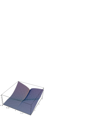
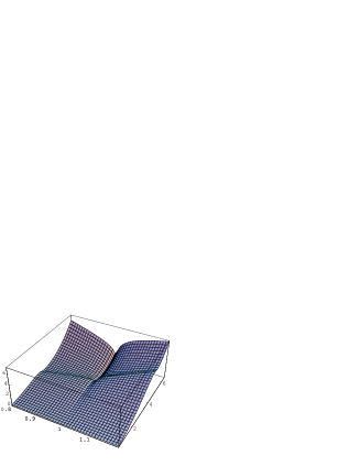
FIG. 1.: Effective potential: $V(\frac{a[u]}{\Lambda},B)$ and $V(\frac{u}{\Lambda^{2}},B)$ as a function of $u=\hbox{tr}\langle\phi^{2}\rangle$ and $B$

FIG. 2.: Dual Effective potential: $V_{D}(\frac{a_{D}[u]}{\Lambda},B)$ as a function of $u$ and $B$

                          

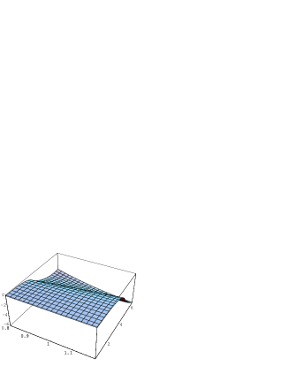
FIG. 3.: Contribution to the effective- and dual effective potential from the non-leading terms as a function of $u$ and $B$

REFERENCES

- [1] N. Seiberg and E. Witten, Nucl. Phys. B426, 19 (1994), (E) B430 (1994) 485.
- [2] N. Seiberg and E. Witten, Nucl. Phys. B431 484 (1994).
-
[3]
M. Matone, Phys. Rev. Lett. 78 1412 (1997);
M. Henningson, Nucl. Phys. bf B458 (1996) 445. - [4] C. Ford and I. Sachs, Phys. Lett. B362 88 (1995).
- [5] A. Yung, Nucl. Phys. B485 38 (1997).
- [6] A. Salam and J. Strathdee, Nucl. Phys. B90, 203 (1975).
-
[7]
R. Flume, M. Magro, L.O’Raifeartaigh, I. Sachs
and O. Schnetz, Nucl. Phys. B494 331 (1997);
M. Magro, L.O’Raifeartaigh, I. Sachs, Nucl.Phys. B508 (1997) 433-448. -
[8]
M.J. Duff and M. Ramon-Medrano, Phys. Rev. D12 (1975) 3357;
I.A. Batalin, S.G. Matinyan, and Savvidy, Sov. J. Nucl. Phys. 26, 214 (1977);
N.K. Nielsen and P. Olesen, Phys. Lett. 79B, 304 (1978). - [9] E.S. Fradkin and A.A. Tseytlin, Nucl. Phys. B227 (1983) 252.
- [10] N.B. Nielsen and M. Ninomiya, Nucl. Phys. B156, 1 (1979).
- [11] C. Flory, SLAC-PUB-3244 (1983).
- [12] H. Leutwyler, Nucl. Phys. B179, 129 (1981).
- [13] P. Cea, Phys. Rev. D37, 1637 (1988).
-
[14]
I.L. Buchbinder, E.I. Buchbinder, E.A. Ivanov,
S.M. Kuzenko and B.A. Ovrut, Phys. Lett. B412 (1997) 309;
I.L. Buchbinder, E.I. Buchbinder, S.M. Kuzenko, B.A. Ovrut, Phys. Lett. B417 (1998) 61;
I.L. Buchbinder, S.M. Kuzenko, B.A. Ovrut, hep-th/9710142. - [15] P. Di Vecchia, R. Musto, F. Nicodemi, and R. Pettorino, Nucl. Phys. B252, 635 (1985).
- [16] K. Fujikawa, B.W. Lee, and A.I. Sanda, Phys. Rev. D6, 2923 (1972).
- [17] S. Hawking, Comm. Math. Phys. 55, 133 (1977).
- [18] D.G.C. McKeon and T.N. Sherry, Phys. Rev. Lett. 59, 532 (1987).
-
[19]
J. Schwinger, Phys. Rev. 82, 664 (1951);
W. Dittrich and M. Reuter, ”Effective Lagrangians in Quantum Electrodynamics,” (Springer-Verlag, NY, 1985). - [20] J. Sapirstein, Phys. Rev. D20, 3246 (1979).
- [21] I.S. Gradshteyn and I.M. Ryzhik, ”Tables of Integrals, Series and Products,” (Academic Press, Boston, 1994).
- [22] D. Kay, PhD Thesis, Simon Fraser U. (1985).
- [23] I. Chepelev, A.A. Tseytlin, Nucl.Phys. B511 (1998) 629.
-
[24]
F. Gliozzi, J. Scherk and D. Olive, Nucl. Phys. B122 (1977) 253;
P. Fayet, Nucl. Phys. B149 (1979) 137; L. Brink, J. Schwarz and J. Scherk, Nucl. Phys. B121 (1977) 77. - [25] J. Honerkamp, Nucl. Phys. B48 (1972) 269.
- [26] M. Dine and N. Seiberg, Phys. Lett. B409 (1997) 239.
- [27] N. Seiberg, Phys. Lett. B206 (1988) 75.
- [28] D. Finnell and P. Pouliot, Nucl. Phys. B453 (1995) 225.
- [29] A. Bilal, hep-th/9601007.
- [30] P.C. West, “Introduction to Supersymmetry and Supergravity”, World Scientific, London, (1990).
-
[31]
I.A. Batalin, A.E. Shabad, JETP 33
(1971) 483;
I. Sachs, PhD thesis, ETH No. 10728 (1994) unpublished;
V.P. Gusynin and I.A. Shovkovy, Can. J. Phys. 74 (1996) 282; hep-th/9804143. - [32] D. Gitman, W. daCruz, and S.I. Zlatev, USP preprint (1995).