Two-Monopole Systems and the Formation of Non-Abelian Clouds

Abstract

We study the energy density of two distinct fundamental monopoles in $SU(3)$ and $Sp(4)$ theories with an arbitrary mass ratio. Several special limits of the general result are checked and verified. Based on the analytic expression of energy density the coefficient of the internal part of the moduli space metric is computed, which gives it a nice “mechanical” interpretation. We then investigate the interaction energy density for both cases. By analyzing the contour of the zero interaction energy density we propose a detailed picture of what happens when one gets close to the massless limit. The study of the interaction energy density also sheds light on the formation of the non-Abelian cloud.

PACS number(s): 11.15.-q, 11.27.+d, 14.80.Hv

I Introduction

Since the pioneering work of t’Hooft and Polyakov [1] a quarter of a century ago, the study of magnetic monopoles in various Yang-Mills-Higgs theories has become a fruitful direction of research. Investigations of these solitonic states have uncovered many deep and beautiful structures of gauge theories and greatly improved our understanding of those theories.

Magnetic monopoles arise when the Higgs configuration has a non-trivial topology at spatial infinity. For a theory with the gauge group $G$ broken into a residue group $H$, topologically non-trivial configurations are possible when the second homotopy group of the vacuum manifold, namely $\Pi_{2}(G/H)$, is non-trivial. Many works have been performed to understand the structure and the metric properties of BPS monopole solutions. It is known that when the unbroken gauge group $H$ is Abelian, generalization from the original single $SU(2)$ monopole to multi-monopole systems in arbitrary gauge theories is quite straightforward (at least conceptually) [2].

When the unbroken gauge symmetry is non-Abelian, however, the situation becomes more complicated. Certain fundamental monopoles (namely the monopoles associated with simple roots of the gauge group) become massless and two cases need to be distinguished: the total magnetic charge carried by monopole is non-Abelian (as the long range magnetic field transforms non-trivially under unbroken symmetry) or purely Abelian. In the former case, as was discussed in [3], various topological pathologies appear and prevent us from defining the non-Abelian charge globally. On the other hand, when the total magnetic charge is Abelian (the latter case), there’s no topological obstacle, everything behaves nicely. Therefore the majority of the works on monopoles in the presence of non-Abelian unbroken symmetry focus this case [4] [5][6][7][8]. The modern picture of such a case is described by the so called non-Abelian cloud arising from the interaction between massless monopoles and massive monopoles.

In spite of the progress in understanding the field configurations and the moduli space metrics, the detailed behavior of the interaction that accounts for the formation of the non-Abelian cloud is still unclear. Under the massless limit, a single monopole will spread out and eventually disappear. This trivial behavior can be significantly changed in the presence of massive monopoles. In the case where the system carries Abelian charge, the would-be massless monopole will lose its identity as an isolated soliton once its core region overlaps with massive monopoles, its size will cease to expand, and its internal structure will change in a way that reflects the restored non-Abelian symmetry. This picture must be distinguished from the case when the system carries non-Abelian charge (in the massless limit). Having a proper detailed description of the two situations will be helpful in understanding the formation of the non-Abelian cloud. In this paper we will try to address some of these issues. We will compare the behavior of two monopole systems in $SU(3)$ and $Sp(4)$ theories since they are the two simplest models containing the interesting contents we are going to study.

The paper is organized as follows: In Sec II, we introduce (as the foundation of our calculation) Nahm’s formalism for the monopole energy density. In Sec III and IV, the energy densities of two (distinct) fundamental monopoles in $SU(3)$ and $Sp(4)$ theories are calculated and verified in several special cases. In Sec IV we compute the internal part of the moduli space metric from a “mechanical” point of view. In Sec V we study the formation of the non-Abelian cloud by analyzing the behavior of the interaction energy density. In Sec VI we conclude with some remarks.

II Nahm’s formalism for the energy density

As was used in many papers, Nahm’s formalism has proved to be a powerful tool in calculating many aspects of monopoles. This method is an analogue of the ADHM construction used in instanton physics [9] and was first proposed by Nahm [10]. Recently Nahm’s formalism has been generalized to deal with calorons (periodic instantons) [11][12], and we will use some of the results developed in those works.

Consider the $SU(N)$ Yang-Mills-Higgs system, assuming the asymptotic Higgs field along a given direction to be $\phi_{\infty}={\rm diag}(\mu_{1},...,\mu_{N})$ (with $\mu_{1}\leq\cdots\leq\mu_{N}$), then the Nahm data for the caloron that carries instanton number $k$ are defined over intervals $(\mu_{1},\mu_{2})$,…, $(\mu_{N-1},\mu_{N})$, $(\mu_{N},\mu_{1}+2\pi/\beta)$ (where $\beta$ is the circumference along the $S^{1}$ direction in space $R^{3}\times S^{1}$) with $\mu_{1}$ and $\mu_{1}+2\pi/\beta$ identified. In each interval the Nahm data are triplets of $k\times k$ Hermitian matrix functions ${\bf T}(t)$ determined by Nahm’s equations and boundary conditions. In this paper we will only use the case with $k=1$ for which Nahm data are triplets of constants representing the positions of the corresponding constituent monopoles. It is known that the action density of instantons (in the usual ADHM method) is given by (it differs from [13] by a sign since we choose $F_{\mu\nu}$ to be Hermitian rather than anti-Hermitian):

$$\rho_{s}={\rm tr}F^{2}_{\mu\nu}=\Box\Box\log\det f$$ (1)

where $f$ is the inverse operator (whose matrix elements form Green’s function) of $\bigtriangleup^{\dagger}\bigtriangleup$ ($\bigtriangleup$ is the usual ADHM matrix), and $\Box$ is a four dimensional Laplacian. For $SU(N)$ calorons similar results can be established using the Fourier transformation of the original ADHM method and one has the following formula for the Green’s function $f(t,t^{\prime})=\langle{t}|f|{t^{\prime}}\rangle$ [11][12]:

$$\left[-\frac{d^{2}}{dt^{2}}+|{\bf x}-{\bf T}(t)|^{2}+\sum_{i}|{\bf T}_{i}-{\bf T}_{i-1}|\delta(t-\mu_{i})\right]f(t,t^{\prime})=\delta(t-t^{\prime})$$ (2)

where the sum is taken over all the boundary points between adjacent intervals. In order to get the Green’s function for monopoles instead of calorons, notice that in the constituent monopole picture of calorons, an additional type of monopole has been introduced to neutralize the magnetic charge, so the usual multi-monopole Green’s function can be obtained by moving the additional monopole to spatial infinity which leads to the following natural boundary conditions:

$$f(\mu_{1},t^{\prime})=f(\mu_{N},t^{\prime})=0$$ (3)

On the other hand, for purely magnetic configurations, the energy density is given by (a factor of $1/2$ is omitted for simplicity):

$$\rho=\rho_{s}=\Box\Box\log\det f$$ (4)

For later convenience, it would be useful to explore Eq.(4) a little bit further. Notice that for an operator $f$:

$$\log\det f={\rm tr}\log f=-{\rm tr}\left[\sum_{n=1}^{\infty}\frac{(1-f)^{n}}{n}\right]$$ (5)

therefore ($i=1,2,3$)

$$\partial_{i}\log\det f={\rm tr}\left\{\left[\sum_{n=0}^{\infty}(1-f)^{n}\right]\partial_{i}f\right\}={\rm tr}(f^{-1}\partial_{i}f)$$ (6)

Further notice that $f=(\bigtriangleup^{\dagger}\bigtriangleup)^{-1}$ (Nahm’s construction operator $\bigtriangleup^{\dagger}$ is defined to be $i\partial_{t}-i({\bf x}-{\bf T})\cdot\sigma$ in each interval), so

$${\rm tr}(f^{-1}\partial_{i}f) = {\rm tr}(\bigtriangleup^{\dagger}\bigtriangleup\partial_{i}f)$$ (7)

$$= {\rm tr}[\partial_{i}(\bigtriangleup^{\dagger}\bigtriangleup f)-f\partial_{i}(\bigtriangleup^{\dagger}\bigtriangleup)]$$ (8)

$$= -\sum_{j}\left[\int dt^{\prime}f(t^{\prime},t^{\prime})\partial_{i}|{\bf x}-{\bf T}_{j}|^{2}\right]$$ (9)

So finally we have obtained a convenient formula for the energy density:

$$\partial_{i}\log\det f=-\sum_{j}\left[\partial_{i}|{\bf x}-{\bf T}_{j}|^{2}\int dt^{\prime}f(t^{\prime},t^{\prime})\right]$$ (10)

where $\partial_{i}|{\bf x}-{\bf T}_{j}|^{2}$ has been moved out from the integration since in each interval ${\bf T}_{j}$ does not depend on $t^{\prime}$ (for the $k=1$ case only). Equation (10) together with Eqs.(2) (3) (4) (in Eq.(4) use three dimensional Laplacian $\bigtriangleup$ to replace $\Box$) forms a framework to compute energy density of monopole systems considered in this paper.

III Two fundamental monopoles in $SU(3)$ theory

The root diagram of $SU(3)$ theory is shown in Fig 1:

FIG. 1.: Root diagram of $SU(3)$ theory

We will consider the system formed by one $\alpha$ and one $\beta$ monopole, $h$ in the graph refers to the Higgs direction along which $\beta$ monopole is massless.

A Energy density

We choose $\phi_{\infty}$ (along a given direction) to be ${\rm diag}(-1-\mu,2\mu,1-\mu)$ (with $-1/3\leq\mu\leq 1/3$), so the masses of the two fundamental monopoles are;

$$m_{\alpha}=1+3\mu;\hskip 14.22636ptm_{\beta}=1-3\mu$$ (11)

Without losing generality, we can place the $\alpha$-monopole on the origin and $\beta$-monopole on $(0,0,{\cal D})$ which is equivalent to choosing ${\bf T}(t)=(0,0,0)$ for $t\in(-1-\mu,2\mu)$ and ${\bf T}(t)=(0,0,{\cal D})$ for $t\in(2\mu,1-\mu)$. Applying Eqs.(2) (3) to this case we have

$$\left[-\frac{d^{2}}{dt^{2}}+|{\bf x}-{\bf T}(t)|^{2}+{\cal D}\delta(t-2\mu)\right]f(t,t^{\prime})=\delta(t-t^{\prime})$$ (12)

$$f(-1-\mu,t^{\prime})=f(1-\mu,t^{\prime})=0$$ (13)

It’s easy to see from these equations that the Green’s function has the following form:

• Case A: $-1-\mu<t^{\prime}<2\mu$

  $$f(t,t^{\prime})=\left\{\begin{array}[]{lc}A\sinh[r(t+1+\mu)]&(-1-\mu<t<t^{\prime})\\ B\sinh(rt)+C\cosh(rt)&(t^{\prime}<t<2\mu)\\ D\sinh[r^{\prime}(1-\mu-t)]&(2\mu<t<1-\mu)\end{array}\right.$$ (17)

• Case B: $2\mu<t^{\prime}<1-\mu$

  $$f(t,t^{\prime})=\left\{\begin{array}[]{lc}A^{\prime}\sinh[r(t+1+\mu)]&(-1-\mu<t<2\mu)\\ B^{\prime}\sinh(r^{\prime}t)+C^{\prime}\cosh(r^{\prime}t)&(2\mu<t<t^{\prime})\\ D^{\prime}\sinh[r^{\prime}(1-\mu-t)]&(t^{\prime}<t<1-\mu)\end{array}\right.$$ (18)

where $r=\sqrt{x_{1}^{2}+x_{2}^{2}+x_{3}^{2}}$, $r^{\prime}=\sqrt{x_{1}^{2}+x_{2}^{2}+(x_{3}-{\cal D})^{2}}$ are distances from two monopoles and the coefficients $A,B,C,A^{\prime},B^{\prime},C^{\prime}$ are all functions of $t^{\prime}$.

In each case Eq.(12) also implies the usual boundary conditions (which we won’t bother writing down) concerning the continuity of $f(t,t^{\prime})$ and the jumps of $\partial_{t}f(t,t^{\prime})$ at each point where the argument of the $\delta$-functions becomes zero. All the coefficients can be computed from those boundary conditions. It’s helpful to notice that Eq.(10) makes use of $f(t,t^{\prime})$ only in the form of $\int dt^{\prime}f(t^{\prime},t^{\prime})$ which is equal to

$$\int dt^{\prime}f(t^{\prime},t^{\prime}) = \int^{2\mu}_{-1-\mu}dt^{\prime}A(t^{\prime})\sinh[r(t^{\prime}+1+\mu)]$$ (19)

$$+ \int^{1-\mu}_{2\mu}dt^{\prime}D^{\prime}(t^{\prime})\sinh[r^{\prime}(1-\mu-t^{\prime})]$$ (20)

and so we only need $A$ and $D^{\prime}$. Computing them using boundary conditions and putting into Eqs.(20) and (10) one obtains the following result:

$$\partial_{i}(\log\det f) = -\hat{r}_{i}\frac{rp\sinh p\sinh q+A_{1}(p\cosh p-\sinh p)}{rM}$$ (21)

$$- \hat{r}^{\prime}_{i}\frac{r^{\prime}q\sinh q\sinh p+A_{2}(q\cosh q-\sinh q)}{r^{\prime}M}$$ (22)

where $p,q,A_{1},A_{2},M$ are defined as:

$$p=m_{\alpha}r;\hskip 14.22636ptq=m_{\beta}r^{\prime}$$ (23)

$$A_{1}={\cal D}\sinh q+r^{\prime}\cosh q;\hskip 14.22636ptA_{2}={\cal D}\sinh p+r\cosh p$$ (24)

$$M={\cal D}\sinh p\sinh q+r\cosh p\sinh q+r^{\prime}\sinh p\cosh q$$ (25)

From Eq.(22) one can also derive the regularized determinant of Green’s function to be

$$(\det f)_{{\rm reg}}=\frac{rr^{\prime}}{M}$$ (26)

which is defined in the sense that it is finite and gives the same $\partial_{i}(\log\det f)$ and energy density $\rho$ through:

$$\partial_{i}(\log\det f)=\partial_{i}[\log(\det f)_{{\rm reg}}]$$ (27)

$$\rho=\bigtriangleup\bigtriangleup\log(\det f)_{{\rm reg}}$$ (28)

Three typical configurations are shown in Fig 2 (we plot it on the $x-z$ plane since the configurations are axially symmetric).

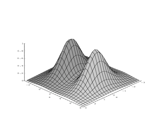
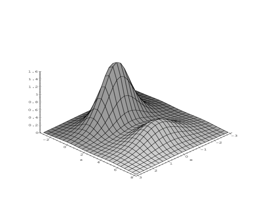
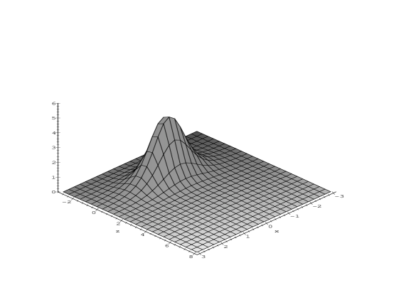
FIG. 2.: Energy density of two fundamental monopoles on the $x-z$ plane in $SU(3)$ theory. $\alpha$ and $\beta$ monopoles are located at $(0,0)$ and $(0,5)$. The mass ratio $m_{\alpha}/m_{\beta}$ (from top to bottom) is chosen to be 1, 1.35 and 3

B Various limits of the energy density

In this subsection let’s check certain limits of the general form of the energy density, this serves as a partial verification of the result obtained in last subsection.

1. ${\cal D}=0$ case (two monopoles are on top of each other):

   In this case we expect (and will see) that the resulting energy density is the same as that of an $SU(2)$-embedded monopole with mass $m=m_{\alpha}+m_{\beta}=2$. Since two monopoles are overlapped, so $r=r^{\prime}$ and one has:

   $$M=r\sinh(2r)$$ (29)

   So (using Eqs.(26)(27))

   $$\partial_{i}(\log\det f)=-\hat{r}_{i}{\rm H}(2r)$$ (30)

   where ${\rm H}(2r)$ is the $m=2$ ($m$ is the mass parameter) case of the single monopole function defined as

   $${\rm H}(mr)=m\left[\coth(mr)-\frac{1}{mr}\right]$$ (31)

   From Eq.(30), one can further get:

   $$\bigtriangleup(\log\det f)=\partial_{i}\partial_{i}(\log\det f)={\rm H}^{2}(2r)-4$$ (32)

   and therefore

   $$\rho=\bigtriangleup\bigtriangleup(\log\det f)=\bigtriangleup[{\rm H}^{2}(2r)]$$ (33)

   which is fully compatible (in the suitable convention of normalization) with another well known formula [14]:

   $$\rho=\bigtriangleup({\rm tr}\phi^{2})$$ (34)

   since $\phi\propto{\rm H}(2r)$ for single $SU(2)$-embedded monopole with mass $m=2$.

2. Massless limit:

   This is the case when one of the monopoles becomes massless (we will investigate this limit in more detail in Sec IV). In our convention this happens when $\mu=\pm 1/3$. Without losing generality, we choose $\mu=1/3$ (so the $\beta$-monopole is massless), then $p=2r$, $q=0$ and

   $$M=r^{\prime}\sinh(2r)$$ (35)

   and therefore

   $$\partial_{i}(\log\det f)=-\hat{r}_{i}{\rm H}(2r)$$ (36)

   which (as the ${\cal D}=0$ case) again leads to the energy density of a single $SU(2)$ monopole with mass $m=2$. Notice $m_{\alpha}=2$ in this case, so such a result means that the $\beta$-monopole doesn’t affect the energy density in the massless limit (which, as we will see, is very different from $Sp(4)$ case).

3. Removing one monopole:

   Again, without losing generality, let’s move the $\beta$-monopole away so that $r^{\prime}\rightarrow\infty$, the dominant term in $M$ is

   $$M\sim r^{\prime}\exp(m_{\beta}r^{\prime})\sinh(m_{\alpha}r)$$ (37)

   which leads to

   $$\partial_{i}(\log\det f)=-\hat{r}_{i}{\rm H}(m_{\alpha}r)-m_{\beta}\hat{r}^{\prime}_{i}$$ (38)

   Since $\hat{r}^{\prime}_{i}$ represents a constant vector at this limit, so Eq.(38) is exactly what one expects for a single monopole with mass $m_{\alpha}$.

IV Two fundamental monopoles in $Sp(4)$ theory

$Sp(4)$ (or equivalently $SO(5)$) theory is the simpest theory to study the non-Abelian cloud. The root diagram is shown in Fig.3:

FIG. 3.: Root diagram of $Sp(4)$ theory. $\beta^{*}$, $\delta^{*}$ are co-roots

Two cases containing massless monopoles have been studied before. When the asymptotic Higgs field is along the $h$ direction, the Abelian configuration is made of two massive $\beta$-monopoles and one massless $\alpha$-monopole [6], when the asymptotic Higgs field is along the $h^{\prime}$ direction, the Abelian configuration is made of one massive $\alpha$-monopole and one massless $\beta$-monopole [5]. In this section we will consider the general energy density for a one $\alpha$ one $\beta$ monopole system (with arbitrary mass ratio) which will help us to see how the massless limit would be eventually achieved.

A Energy density

We choose $\phi_{\infty}$ (along a given direction) to be ${\rm diag}(-1,-\mu,\mu,1)$ (with $0\leq\mu\leq 1$), so the masses of the fundamental monopoles are:

$$m_{\alpha}=2-2\mu;\hskip 14.22636ptm_{\beta}=2\mu$$ (39)

The monopole locations are chosen to be the same as in the $SU(3)$ case. As we know, in Nahm’s method $Sp(4)$ theory is embedded into $SU(4)$ theory whose Nahm data satisfy symmetric constraints [6], in our convention the $SU(4)$ Nahm data are given by ${\bf T}(t)=(0,0,0)$ for $t\in(-1,-\mu)\cup(\mu,1)$ and ${\bf T}(t)=(0,0,{\cal D})$ for $t\in(-\mu,\mu)$. Applying Eqs.(2) (3) to this case we have:

$$\left[-\frac{d^{2}}{dt^{2}}+|{\bf x}-{\bf T}(t)|^{2}+{\cal D}\delta(t+\mu)+{\cal D}\delta(t-\mu)\right]f(t,t^{\prime})=\delta(t-t^{\prime})$$ (40)

$$f(-1,t^{\prime})=f(1,t^{\prime})=0$$ (41)

The Green’s function satisfying these equations has the following form:

• Case A: $-1<t^{\prime}<-\mu$

  $$f(t,t^{\prime})=\left\{\begin{array}[]{lc}A\sinh[r(t+1)]&(-1<t<t^{\prime})\\ B\sinh(rt)+C\cosh(rt)&(t^{\prime}<t<-\mu)\\ D\sinh(r^{\prime}t)+E\cosh(r^{\prime}t)&(-\mu<t<\mu)\\ F\sinh[r(1-t)]&(\mu<t<1)\end{array}\right.$$ (46)

• Case B: $-\mu<t^{\prime}<\mu$

  $$f(t,t^{\prime})=\left\{\begin{array}[]{lc}A^{\prime}\sinh[r(t+1)]&(-1<t<-\mu)\\ B^{\prime}\sinh(r^{\prime}t)+C^{\prime}\cosh(r^{\prime}t)&(-\mu<t<t^{\prime})\\ D^{\prime}\sinh(r^{\prime}t)+E^{\prime}\cosh(r^{\prime}t)&(t^{\prime}<t<\mu)\\ F^{\prime}\sinh[r(1-t)]&(\mu<t<1)\end{array}\right.$$ (51)

• Case C: $\mu<t^{\prime}<1$

  $$f(t,t^{\prime})=\left\{\begin{array}[]{lc}A^{\prime\prime}\sinh[r(t+1)]&(-1<t<-\mu)\\ B^{\prime\prime}\sinh(r^{\prime}t)+C^{\prime\prime}\cosh(r^{\prime}t)&(-\mu<t<\mu)\\ D^{\prime\prime}\sinh(rt)+E^{\prime\prime}\cosh(rt)&(\mu<t<t^{\prime})\\ F^{\prime\prime}\sinh[r(1-t)]&(t^{\prime}<t<1)\end{array}\right.$$ (56)

where $r$ and $r^{\prime}$ have the same meaning as before, and $A,...,F^{\prime\prime}$ are all functions of $t^{\prime}$.

Similarly as in the $SU(3)$ case, we only need some of the coefficients ($A$, $B^{\prime}$, $C^{\prime}$, $D^{\prime\prime}$) which (as well as all other coefficients) can be determined by boundary conditions coming from the $\delta$-functions in Eqs.(40). Compute them and putting them into Eqs.(10) one obtains:

$$\partial_{i}(\log\det f)=-\hat{r}_{i}\frac{PA_{1}+QA_{2}}{\cosh rP+\sinh rQ}-\hat{r}^{\prime}_{i}\left(\frac{MB_{1}}{L}+\frac{LB_{2}}{M}\right)$$ (57)

where the following functions are introduced:

$$u=(1-\mu)r;\hskip 14.22636ptv=\mu r;\hskip 14.22636ptw=\mu r^{\prime}$$ (58)

$$A_{1} = \frac{-\cosh r+\cosh(u-v)}{r}+2(1-\mu)\sinh r$$ (59)

$$A_{2} = \frac{-\sinh r-\sinh(u-v)}{r}+2(1-\mu)\cosh r$$ (60)

$$B_{1}=\mu+\frac{\sinh(2\mu r^{\prime})}{2r^{\prime}};\hskip 14.22636ptB_{2}=\mu-\frac{\sinh(2\mu r^{\prime})}{2r^{\prime}}$$ (61)

$$L = {\cal D}\sinh u\cosh w+r\cosh u\cosh w+r^{\prime}\sinh u\sinh w$$ (62)

$$M = {\cal D}\sinh u\sinh w+r\cosh u\sinh w+r^{\prime}\sinh u\cosh w$$ (63)

$$N_{1} = {\cal D}\sinh v\sinh w-r\cosh v\sinh w+r^{\prime}\sinh v\cosh w$$ (64)

$$N_{2} = {\cal D}\cosh v\sinh w-r\sinh v\sinh w+r^{\prime}\cosh v\cosh w$$ (65)

$$N_{3} = {\cal D}\sinh u\sinh(2w)+r\cosh u\sinh(2w)+r^{\prime}\sinh u\cosh(2w)$$ (66)

$$P=r^{\prime}\sinh vM-N_{1}N_{3};\hskip 14.22636ptQ=-r^{\prime}\cosh vM+N_{2}N_{3}$$ (67)

The reguralized determinant of The Green’s function from Eq.(57) is

$$(\det f)_{{\rm reg}}=\frac{r^{2}r^{\prime}}{LM}$$ (68)

Three typical configurations are shown in Fig 4.

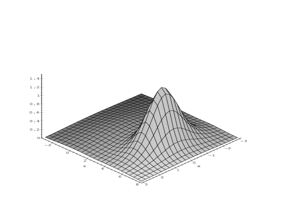
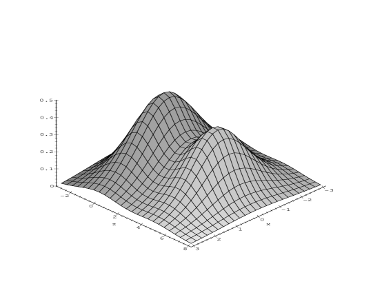
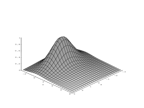
FIG. 4.: Energy density of two fundamental monopoles on the $x-z$ plane in $Sp(4)$ theory. $\alpha$ and $\beta$ monopoles are located at $(0,0)$ and $(0,5)$. Mass ratio $m_{\alpha}/m_{\beta}$ (from top to bottom) is chosen to be 1, 2 and 4

One can see that the energy density of the two fundamental monopoles in $Sp(4)$ theory is not symmetric, this is because here $\alpha$ and $\beta$ monopoles have different energy distributions. As we know, the mass of $SU(2)$-embedded $\gamma$-monopoles in arbitrary gauge theory is given by $h\cdot\gamma^{*}$ while the scale of such monopoles is determined by $1/(h\cdot\gamma)$ ($\gamma$ is the root to which the $SU(2)$-embedded monopoles are associated, $h$ is the asymptotic Higgs direction). As a consequence, in $Sp(4)$ theory when $\alpha$ and $\beta$ monopoles have the same mass, the scale of the $\beta$-monopole is only half of the scale of the $\alpha$-monopole therefore the maximal energy density is eight times that of the $\alpha$-monopole, this is why in the plotting with $m_{\alpha}:m_{\beta}=1$ one can hardly see the $\alpha$-monopole.

B Various limits of the energy density

The expression of the energy density of the two fundamental monopoles in $Sp(4)$ theory is much more complicated than in the $SU(3)$ case, to see its correctness, let’s check several special cases.

1. ${\cal D}=0$ case (two monopoles are on top of each other):

   In this case we again expect an $SU(2)$-embedded monopole with mass $m=m_{\alpha}+m_{\beta}=2$. Since $r=r^{\prime}$, one gets

   $$L=r\cosh r;\hskip 14.22636ptM=r\sinh r$$ (69)

   which generates the familar result:

   $$\partial_{i}(\log\det f)=-\hat{r}_{i}{\rm H}(2r)$$ (70)

   which is the same as Eq.(30), so in this limit the result is exactly what we expected.

2. Massless limit:

   We are interested in the limit when the total magnetic charge is Abelian which is realized by $\mu\rightarrow 0$ (when the $\beta$-monopole becomes massless). In this limit one has

   $$L={\cal D}\sinh r+r\cosh r;\hskip 14.22636ptM=r^{\prime}\sinh r$$ (71)

   which leads to

   $$\partial_{i}(\log\det f)=-\hat{r}_{i}\frac{2r^{2}\cosh(2r)+2{\cal D}r\sinh(2r)-r\sinh(2r)-2{\cal D}\cosh(2r)+2{\cal D}}{r^{2}\sinh(2r)+{\cal D}r\cosh(2r)-{\cal D}r}$$ (72)

   On the other hand, the Higgs configuration in this limit is given in [7][8], in that work, the Higgs configuration of $N-1$ fundamental monopoles is calculated in the symmetry breaking pattern $SU(N)\rightarrow U(1)\times SU(N-2)\times U(1)$. The relevant $Sp(4)$ Higgs configuration can be obtained by taking the $N=4$ case and putting two massive monopoles on top of each other. In a proper normalization the result of [7] (after simplification) can be written as (where $\sigma_{r}=\sigma\cdot\hat{r}$)

   $$\phi=\frac{1}{\sqrt{2}}\left(\begin{array}[]{cc}{\rm H}(2r)\sigma_{r}&\sqrt{\frac{2{\cal D}\tanh^{2}r}{\sinh(2r)(r+{\cal D}\tanh r)}}\\ \sqrt{\frac{2{\cal D}\tanh^{2}r}{\sinh(2r)(r+{\cal D}\tanh r)}}&\frac{2{\cal D}r-{\cal D}\sinh(2r)}{2r\cosh^{2}r(r+{\cal D}\tanh r)}\sigma_{r}\end{array}\right)$$ (73)

   which leads to

   $${\rm tr}\phi^{2}={\rm H}^{2}(2r)+\frac{4{\cal D}\tanh^{2}r}{\sinh(2r)(r+{\cal D}\tanh r)}+\left[\frac{2{\cal D}r-{\cal D}\sinh(2r)}{2r\cosh^{2}r(r+{\cal D}\tanh r)}\right]^{2}$$ (74)

   As we did before, in order to show that Eqs.(4) (72) and (34) (74) give the same result it is sufficient to show that the difference between $\partial_{i}\partial_{i}(\log\det f)$ and ${\rm tr}\phi^{2}$ is constant. This is messy, but one can verify that

   $$\partial_{i}\partial_{i}(\log\det f)={\rm tr}\phi^{2}-4$$ (75)

   so the massless limit works out correctly. Unlike the $SU(3)$ case, the massless limit of $Sp(4)$ theory is rather non-trivial (the non-Abelian cloud coming into playing).

   One can easily show that when the $\alpha$-monopole becomes massless (in that case the total magnetic charge is non-Abelian), the situation is similar to the $SU(3)$ case, namely the energy density is equal to the energy density of a single $\beta$-monopole.

3. Removing the $\alpha$-monopole:

   Now let’s check what happens when one monopole is removed. Since the two monopoles are not symmetric in the $Sp(4)$ case so we check them separately. When ${\cal D}\rightarrow\infty$ but keeping $r^{\prime}$ finite (therefore $r\rightarrow\infty$), the $\alpha$-monopole is removed. The leading contributions of $L,M$ are:

   $$L\sim r\exp[(1-\mu)r]\cosh(\mu r^{\prime});\hskip 14.22636ptM\sim r\exp[(1-\mu)r]\sinh(\mu r^{\prime})$$ (76)

   Putting these into Eqs.(68) and (27) one obtains:

   $$\partial_{i}(\log\det f)=-\hat{r}^{\prime}_{i}{\rm H}(2\mu r^{\prime})-m_{\alpha}\hat{r}_{i}$$ (77)

   This (notice that $\hat{r}_{i}$ is a constant vector at this limit) represents an $SU(2)$-embedded monopole with mass $m=m_{\beta}$ which is what we are expecting.

4. Removing the $\beta$-monopole:

   When ${\cal D}\rightarrow\infty$, $r^{\prime}\rightarrow\infty$, the $\beta$ monopole is removed. The leading contributions of $L,M$ are

   $$L\sim M\sim r^{\prime}\exp(\mu r^{\prime})\sinh[(1-\mu)r]$$ (78)

   which lead to (again, the second term is a constant vector at this limit)

   $$\partial_{i}(\log\det f)=-2\hat{r}{\rm H}[(1-\mu)r]-m_{\beta}\hat{r}^{\prime}_{i}$$ (79)

   The energy density coming from this expression is the same as two directly superposed $SU(2)$ monopoles with mass $m=1-\mu=m_{\alpha}/2$. This is consistent with the $SU(4)$ picture introduced in the discussion of the massless limit, namely the $\alpha$ monopole can be considered as the two overlapped $SU(4)$ monopoles whose energy densities are simply added since they are non-interacting. This also gives a direct demonstration of our discussion at the end of subsection A.

C From the moment of inertia to the moduli space metric

Since we have the analytic form of energy density, we are now able to compute the internal part of the moduli space metric using a nice “mechanical” interpretation. The idea of using a mechanical interpretation can be traced to Manton’s original work [15] (where the concept of the moduli space metric itself was introduced by comparing the action of the monopole system and mechanical system) and was used in certain arguments in recent works [6][16]. In this subsection we will consider the massless limit of our $Sp(4)$ system. The metric in this case is known to be [5] (changed into our convention):

$$ds^{2}=md{\bf x}^{2}+\frac{16\pi^{2}}{m}d\chi^{2}+\frac{4\pi}{{\cal D}}d{\cal D}^{2}+4\pi{\cal D}(\sigma_{1}^{2}+\sigma_{2}^{2}+\sigma_{3}^{2})$$ (80)

where $m$ is the total mass (which is just the mass of the $\alpha$-monopole in this case) of the system, $\sigma_{1},\sigma_{2}$ and $\sigma_{3}$ are 1-forms defined as

$$\sigma_{1} = -\sin\psi d\theta+\cos\psi\sin\theta d\phi$$ (81)

$$\sigma_{2} = \cos\psi d\theta+\sin\psi\sin\theta d\phi$$ (82)

$$\sigma_{3} = d\psi+\cos\theta d\phi$$ (83)

with the Euler angles $\theta,\phi$ and $\psi$ having periodicities $\pi,2\pi$ and $4\pi$, respectively. It’s interesting to notice that the last term in Eq.(80) has a “mechanical interpretation” as the rotational energy associated with the massless cloud with the coefficient $4\pi{\cal D}$ playing the role of the moment of inertia of the cloud. To see this let’s calculate the moment of inertia of the non-Abelian cloud. As we know, for a spherically symmetric system the moment of inertia tensor has the form $I_{ij}=I\delta_{ij}$ with

$$I=\frac{2}{3}\int dVr^{2}\rho$$ (84)

Since the rotation of the cloud is actually the gauge rotation in internal space, we should remove the gauge invariant part $\rho({\cal D}=0)$ (this is an $SU(2)$-embedded $\gamma$-monopole which is gauge invariant), so the effective energy density relevant to the internal rotation is $\rho({\cal D})-\rho(0)$. Using the result obtained in the last subsection one can verify that

$$I = \frac{2}{3}\int dVr^{2}[\rho({\cal D})-\rho(0)]$$ (85)

$$= \frac{8\pi}{3}\int drr^{4}[\rho({\cal D})-\rho(0)]$$ (86)

$$= 16\pi{\cal D}$$ (87)

which leads to a term $16\pi{\cal D}(d\omega_{1}^{2}+d\omega_{2}^{2}+d\omega_{3}^{2})$ in the moduli space metric. Here 1-forms $d\omega_{1},d\omega_{2}$ and $d\omega_{3}$ are defined in the group space of $SU(2)$ (namely $S^{3}$). To compare with the last term of Eq.(80) one notices that

$$\sigma_{1}^{2}+\sigma_{2}^{2}+\sigma_{3}^{2}=d\theta^{2}+d\phi^{2}+d\psi^{2}+2\cos\theta d\phi d\psi$$ (88)

therefore the volume of $(\theta,\phi,\psi)$ space is ($g=\det(g_{ij})$ is the determinant of metric matrix coming from Eq.(88))

$${\cal V}=\int\sqrt{|g|}d\theta d\phi d\psi=16\pi^{2}$$ (89)

Since the volume of group space $S^{3}$ is $2\pi^{2}$ the two sets of 1-forms are related by $\sigma_{i}=2d\omega_{i}$ ($i=1,2,3)$. Taking this into account we see that $16\pi{\cal D}(d\omega_{1}^{2}+d\omega_{2}^{2}+d\omega_{3}^{2})$ computed from the moment of inertia is in accordance with the last term in Eq.(80) obtained using other methods.

V Interaction energy density and the formation of the non-Abelian cloud

In previous sections we have calculated the energy density of two monopole systems in $SU(3)$ and $Sp(4)$ theory. We’ve already known that when one approaches the massless limit, the situations are very different depending on the total magnetic charge. If the total magnetic charge is non-Abelian, the resulting energy density is simply the same as the energy density of the massive monopole. When the total magnetic charge is purely Abelian, however, the energy density distribution is deeply affected by the existence of massless monopoles. In the latter case, there is a non-Abelian cloud surrounding the massive monopole, neutralizing the non-Abelian components of the magnetic charge. In this section we want to have a close look at the evolution of the energy density when one approaches the massless limit.

There’s no unique choice of quantity to describe the formation of the non-Abelian cloud, nor is there any unambiguous definition of the non-Abelian cloud itself. But physically there is no doubt that it is the interaction between massive and massless monopoles that determines the behavior of the system, including the formation of the cloud. Our strategy is to study the interaction energy density defined as

$$\rho_{{\rm int}}=\rho_{{\rm total}}-\rho_{\alpha}-\rho_{\beta}$$ (90)

where $\rho_{\alpha}$ and $\rho_{\beta}$ are the energy density of isolated $\alpha$ and $\beta$ monopoles. $\rho_{{\rm int}}$ describes the change of energy distribution caused by the interaction between two monopoles. In particular we will look at the contour of the zero interaction energy density which gives information on where interaction gathers energy and from where it extracts energy.

We have used Maple to generate numerical data and plotted several typical contours (shown in Figs 5, 6) for $SU(3)$ and $Sp(4)$ theories (the region enclosed by the contour has a positive interaction energy density).

FIG. 5.: Contour diagrams of the zero interaction energy density on the $x-z$ plane for $SU(3)$ theory. $\alpha$ and $\beta$ monopoles are located at $(0,0)$ and $(0,10)$, mass ratios $m_{\alpha}:m_{\beta}$ are choosen to be (from top to bottom) 4, 7, 19, 199

FIG. 6.: Contour diagrams of the zero interaction energy density on the $x-z$ plane for $Sp(4)$ theory. $\alpha$ and $\beta$ monopoles are located at $(0,0)$ and $(0,10)$, mass ratios $m_{\alpha}:m_{\beta}$ are choosen to be (from top to bottom) 4, 19, 66, 99

From the contour diagrams one can see the major difference between the two theories when approaching the massless limit. In both cases we start with a simply connected contour for the small mass ratio (when the distance between two monopoles is large, the starting contour could be different). The contour deforms and grows when the mass ratio increases, in both cases it breaks into two disjoint pieces when mass ratio is sufficiently large. The reason it breaks can be understood by directly analyzing the massless limit of $\rho_{{\rm int}}$ (in the $SU(3)$ case $\rho_{{\rm int}}$ itself vanishes but one can use $\rho_{{\rm int}}/m_{\beta}$ which remains finite), Figs 7, 8 show those limits:

FIG. 7.: $\rho_{\rm int}/m_{\beta}$ in $SU(3)$ theory at the massless limit (this curve is independent of ${\cal D}$)

FIG. 8.: $\rho_{\rm int}$ in $Sp(4)$ theory at the massless limit for ${\cal D}=10$ (this curve has a weak dependence on ${\cal D}$)

In both cases the limiting interaction energy density becomes negative outside the core of the $\alpha$-monopole, this means that the contour can’t keep growing and remains simply connected all the way as one increases the mass ratio. After the breaking point, the part of the contour that surrounds the $\alpha$-monopole is stabilized, but the other part undergoes a very different evolution in the two cases: In the $SU(3)$ case that part of the contour keeps growing, but gradually moves away from the $\alpha$-monopole (because of the scale of the graphs, it might not be able to see that easily, but the shortest distance between the two parts of the contour is increasing). In the $Sp(4)$ case, however, the situation is the opposite, the other part of the contour eventually shrinks and finally disappears (this happens before going to the limit). It should be mentioned that in $Sp(4)$ case if the $\beta$-monopole is inside the core of the $\alpha$-monopole, the contour could shrink and be stabilized without breaking into two pieces at first.

The difference in the contour diagram of the two cases explains their different massless limits and accounts for the formation of the non-Abelian cloud. Although in both cases, the interaction alters the energy distribution by accumulating energy in certain regions, in the case of $SU(3)$ that region is ever expanding and the effect of the interaction (therefore the massless monopole itself) is smeared out over the infinitely large area, so the final energy density is completely dominated by the remaining massive monopole. On the other hand, in the $Sp(4)$ case, the interaction extracts energy and deposits it into a small region (in some sense one can say that the interaction is more “localized” in this case), as a result it affects the energy density distribution significantly, and because of the interaction the massless monopole doesn’t grow into infinite size as it would if isolated. The non-Abelian cloud is just the effect of such an interaction.

VI Conclusions

So far we have analyzed the energy density of two monopole systems in $SU(3)$ and $Sp(4)$ theories and obtained some idea on how the massless cloud forms. Based on these results one can make some qualitative conjectures on what might happen in general cases where the interaction energy can be defined as

$$\rho_{{\rm int}}=\rho_{{\rm total}}-\rho_{{\rm massive}}-\rho_{{\rm massless}}$$ (91)

The basic property of $\rho_{{\rm int}}$ we learned from the previous observation is that when the total magnetic charge is purely Abelian, the interaction is more “localized” in contrast to the opposite case. Such an interaction extracts energy from distant regions, accumulates it in the vicinity of massive monopoles and gradually builds up the structure of the non-Abelian cloud. This is fairly similar to the $Sp(4)$ case.

When the total magnetic charge is non-Abelian, however, qualitatively different situations could arise in general. To see this, let’s look at the case with the symmetry breaking pattern $SU(N)\rightarrow U(1)\times SU(N-2)\times U(1)$ ($N>4$). Let $\alpha_{1},...,\alpha_{N-1}$ denote simple roots. When the system contains massive $\alpha_{1}$, $\alpha_{N-1}$ and would be massless $\alpha_{i}$ ($i=2,...,N-3$) monopoles (notice that the $\alpha_{N-2}$-monopole is absent and so the total magnetic charge of the system is non-Abelian), only massive monopoles survive at the massless limit. This can be seen by noticing that the system under consideration is equivalent to the system studied in [8] (which contains the $\alpha_{N-2}$-monopole as well and so the total magnetic charge is Abelian) with the $\alpha_{N-2}$-monopole removed. From [8] we know that the only cloud parameter of the system is given by

$${\cal D}=\sum_{i=2}^{N-1}|{\bf x}_{i}-{\bf x}_{i-1}|$$ (92)

So removing any massless monopole is equivalent to removing the whole cloud (since it makes the cloud size infinity) therefore only massive monopoles survive. This situation is similar to the $SU(3)$ case we have studied. But there are other systems which don’t show such a direct analogue. As an example we can go back to our $Sp(4)$ theory, and consider a system with $N$ massive $\alpha$-monopoles and $N-1$ would be massless $\beta$-monopoles (so the total magnetic charge is non-Abelian). At massless limit, the massless monopoles in this system will form a non-Abelian cloud rather than disappearing. This is because such system can be obtained by removing one $\beta$-monopole from a system containing $N$ $(N>1)$ $\alpha-\beta$ pairs. At the massless limit the latter system contains a non-Abelian cloud with many independent size parameters. Removing one $\beta$-monopole will not make all these parameters infinity and therefore will not destroy the whole cloud. Another way to understand this is to notice that when the extra $\alpha$-monopole is removed, we are left with a system made of $N-1$ $\alpha-\beta$ pairs (it can be called an Abelian sub-system) which certainly contains the non-Abelian cloud. Since removing the $\alpha$-monopole won’t create cloud, the cloud must exist in the original system. This argument can be generalized.

These examples reveal the complexity of the general cases. It seems that at the massless limit a system with a non-Abelian total magnetic charge can still contain massless monopoles (in the form of a non-Abelian cloud) in a “maximal Abelian sub-system”. We think further considerations on such situations will be interesting.

Note added: While writing this paper, we noticed the appearance of [17] from which the energy density of $SU(3)$ and $Sp(4)$ monopoles can also be obtained.

Acknowledgments

The author wishes to thank Kimyeong Lee for useful discussions. This work is supported in part by the U.S. Department of Energy.

REFERENCES

- [1] G t’Hooft, Nucl. Phys. B79 (1974) 276; A. M. Polyakov, JETP Lett. 20 (1974) 194.
- [2] P. Goddard, J. Nuyts and D. Olive, Nucl. Phys. B125 (1977) 1; E. J. Weinberg, Nucl. Phys. B167 (1980) 500.
- [3] A. Abouelsaood, Nucl. Phys. B226 (1983) 309; P. N. Nelson and A. Manohar, Phys. Rev. Lett. 50 (1983) 943; A. Balachandran et al, Phys. Rev. Lett. 50 (1983) 1553.
- [4] A. S. Dancer, Nonlinearity 5 (1992) 1355; A. S. Dancer, Comm. Math. Phys. 158 (1993) 545.
- [5] K. Lee, E. J. Weinberg and P. Yi, Phys. Rev. D54 (1996) 6351.
- [6] K. Lee, C. Lu, Phys. Rev. D57 (1998) 5260.
- [7] E. J. Weinberg, Phys. Lett. 119B (1982) 151.
- [8] E. J. Weinberg and P. Yi, “Explicit Multimonopole Solutions in Gauge Theory”, hep-th/9803164.
- [9] M. F. Atiyah et al, Phys. Lett. 65A (1978) 185.
- [10] W. Nahm, Phys. Lett. 90B (1980) 413; in Monopoles in Quantum Field Theory, edited by N. S. Cragie et al (World Scientific, Singapore, 1982); in Structural Elements in Particle Physics and Statistical Mechanics, edited by J. Honerkamp et al (Plenum, New York, 1983); in Group Theoretical Methods in Physics, edited by G. Denardo et al (Springer-Verlag, Berlin, 1984).
- [11] K. Lee, Phys. Lett. 426B (1998) 323; K. Lee and C. Lu, Phys. Rev. D58 (1998) 025011.
- [12] T. C. Kraan and P. van Baal, Phys. Lett. 428B (1998) 268, hep-th/9802049; “Periodic Instantons with non-trivial Holonomy”, hep-th/9805168.
- [13] H. Osborn, Ann. Phys. (N. Y.) 135 (1981) 373; E. Corrigan and P. Goddard, Ann. Phys. (N. Y.) 154 (1984) 253.
- [14] R. S. Ward, Comm. Math. Phys. 79 (1981) 317.
- [15] N. S. Manton, Phys. Lett 110B (1982) 54.
- [16] P. Irwin, Phys. Rev. D56 (1997) 5200.
- [17] T. C. Kraan and P. van Baal, “Monopole Constituents inside Calorons”, hep-th/9806034.